Rochester Institute of Technology Rochester Institute of Technology

RIT Scholar Works RIT Scholar Works

Theses

1990

Ray tracing for constructive solid modeling Ray tracing for constructive solid modeling

Anju Sharma McCanna

Follow this and additional works at: https://scholarworks.rit.edu/theses

Recommended Citation Recommended Citation McCanna, Anju Sharma, "Ray tracing for constructive solid modeling" (1990). Thesis. Rochester Institute of Technology. Accessed from

This Thesis is brought to you for free and open access by RIT Scholar Works. It has been accepted for inclusion in Theses by an authorized administrator of RIT Scholar Works. For more information, please contact ritscholarworks@rit.edu.

Rochester Institute of TechnologyDepartment of Computer Science

Ray Tracing for Constructive Solid Modeling

by

Anju Sharma McCanna

A thesis, submitted toThe Faculty of the Department of Computer Science,

In partial fulfillment of the requirements for the degree ofMaster of Science in Computer Science.

Approved by:

Dr. Andrew T. Kitchen

S/02Jjl?fGProf. Nan Schaller

JlJ MJ (~cr'{)

Dr. Peter G. Anderson

May 29, 1990

Title of Thesis: Ray Tracing for Constructive Solid Modeling

I, Anju Sharma McCanna, hereby grant permission to the Wallace

Memorial Library, of RIT, to reproduce my thesis In whole or in

part. Any reproduction will not be for commercial use or profit.

11 -

CONTENTS

Title Page

Contents

Abstract

Acknowledgements

PAGE

i

ii

iv

v

1 Introduction 1

1.1 Implementation Techniques 6

1.2 Reasons For Using Ray Tracing 16

1.3 Problem Statement 18

2 Historical Background 19

2.1 Solid Modeling 19

2.2 Ray Tracing 2 9

2.3 Dithering 3 2

3 Implementation Details 3 6

3.1 Relational Database 3 8

3.1.1 User Interface Functions 4 7

3.2 Graphic Application Functions 5 3

Ul

3.3 Ray Tracing Algorithm For Processing

A CSG Tree 5 9

3.3.1 Data Structures 6 0

3.3.2 Selection Of Intersection Points 6 1

3.3.3 Bounding Volumes 6 4

3.4 The Illumination Model 6 6

3.5 Graphics Display Program 6 8

3.6 Helpful Hints 6 9

3.7 Installation Of New Primitive Types 7 1

3.8 Installation Of New Fields 8 0

4 Conclusions 8 3

4.1 Summary 8 3

4.2 Solutions To Problems Encountered 8 6

4.3 Deficiences 8 8

4.4 Future Extensions 8 9

4.5 Related Thesis Topics 9 4

References 9 5

- IV

ABSTRACT

This thesis describes a system for the creation and realistic

depiction of non-geometric, complex, three dimentional solid

models by utilizing a ray tracing algorithm and a graphics

relational database. Geometric primitives such as a sphere,

cylinder, block, and cone are combined together by using the

boolean set operations of union (+), intersection (&), and

difference (-). The three dimentional solid models are built based

on the concept of constructive solid geometric modeling. The

database provides functions for the creation, transformation, and

deletion of the primitives and models. A model may be displayed

as a wireframe for a fast display or as a shaded solid for a

realistic display.

- V

ACKNOWLEDGEMENTS

My thanks to Dr. Andrew T. Kitchen, Prof. Nan C. Schaller,

and Dr. Donald L. Kreher for their support and ideas. My thanks

to my parents, Mrs. Malti Sharma and (late) Dr. Virendra Nath

Sharma for their inspiration, encouragement, and support. I am

grateful to Frank, my husband, for his moral support, and for his

help in finding the "Programmer's Guide to the EGA/VGA". I am

specially grateful to Nikhil, my son, for being so patient.

CHAPTER 1 INTRODUCTION

Solid modeling (SM) systems provide an effective and

versatile means for communicating 3-D object information.

These systems have received much attention in scientific and

engineering applications and have been used in industry and

academia by skilled professionals [Gujar]. However, the

development of SM systems for the non-professional graphics

user has been slow. The reasons for this have been: the high

cost of hardware, inadequate operating environments, and the

lack of a standard, user friendly interface with the system (such

as a graphical window interface). Non-professional graphics

users, in the fields of business, communications, art, science,

engineering, etc., have been using desktop graphics. The term

desktop graphics refers to applications for painting, drawing,

making graphs, and using spreadsheets. These tools became

available when personal computers were developed [Cline]

[McDougal]. Development of SM systems for non-professional

graphics users can provide a wide scope of applications in areas

such as: desktop presentation, architectural design, advertising,

and simulation.

Recently, the cost of high-resolution graphics hardware

has decreased and microcomputers have become faster.

Contemporary, single processor microcomputers can handle

image synthesis of fairly complex 3-D models. In addition,

much progress has been made in the development of

multiprocessor systems. These systems allow more complex

3-D models (static or animated) to be processed faster and with

more ease.

A solid modeling system for a non-professional graphics

user requires a design and implementation that:

(1) is easy to understand and work with;

(2) facilitates the creation and display of realistic, 3-D

solid models; and

(3) facilitates the modification and maintenance of these

models.

In solid modeling, several methods have been developed for the

construction of complex 3-D objects. Most solid modeling

systems have used either one or a combination of the following

methods: constructive solid geometry (CSG), boundary

representation [Mortenson], and sweep techniques [Requicha].

The CSG method is discussed next and the other two methods

are discussed in chapter 2, Historical Background, section 2.1.

The CSG method is most appropriate for SM systems for

non-professional graphics users, because the concept of CSG is

easy to understand. CSG is one of the least complicated methods

to implement by using a ray tracing algorithm. Use of a ray

tracing algorithm to implement CSG results in the creation of

realistic solid models. For modification and maintenance of

solid models, CSG is very suitable for integration with a

relational database.

CSG modeling is object oriented. In CSG modeling,

construction of a complex 3-D object is performed in object

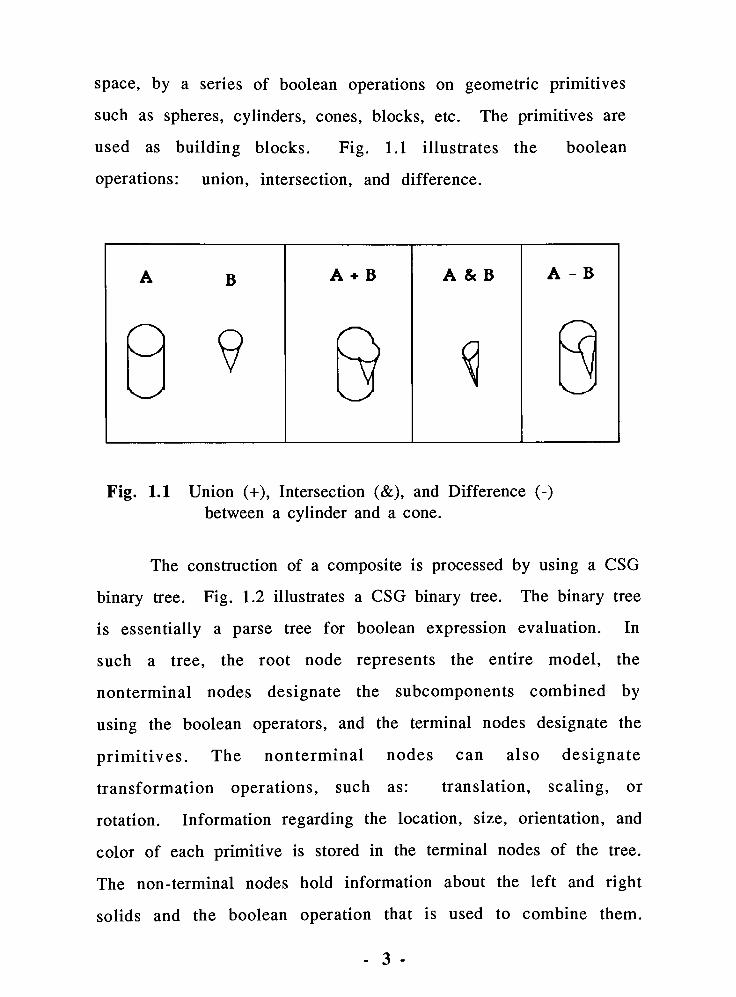
space, by a series of boolean operations on geometric primitives

such as spheres, cylinders, cones, blocks, etc. The primitives are

used as building blocks. Fig. 1.1 illustrates the boolean

operations: union, intersection, and difference.

B

9

A + B A &B A - B

N

Fig. 1.1 Union (+), Intersection (&), and Difference (-)

between a cylinder and a cone.

The construction of a composite is processed by using a CSG

binary tree. Fig. 1.2 illustrates a CSG binary tree. The binary tree

is essentially a parse tree for boolean expression evaluation. In

such a tree, the root node represents the entire model, the

nonterminal nodes designate the subcomponents combined by

using the boolean operators, and the terminal nodes designate the

primitives. The nonterminal nodes can also designate

transformation operations, such as: translation, scaling, or

rotation. Information regarding the location, size, orientation, and

color of each primitive is stored in the terminal nodes of the tree.

The non-terminal nodes hold information about the left and right

solids and the boolean operation that is used to combine them.

3 -

Following is the boolean expression evaluation of the parse tree

given in Fig. 1.2:

abed

=> abc & d

=> (ab -

c) & d

=> ((b + a)-

c) & d

abed

abed

I( & )

/\abc d

I( - )

y\ab c

I(+ )

/\b a

A parse tree for

boolean expression

evaluation

< + )

FT

Pictorial Version

Fig. 1.2 A CSG binary tree.

1.1 IMPLEMENTATION TECHNIQUES

Two major issues in the constructive solid modeling

process are the implementation of the boolean operations: union,

intersection, and difference, and the representation of geometric

objects. There are several techniques for implementing the

boolean operations. These include: the set membership

classification method, the triangulation of potentially intersecting

faces, a hierarchic boundary representation scheme, the directed

loop technique, and the ray tracing (or ray casting) technique.

Set membership classification method [Tilove]: A

membership classification is a function which operates on a pair

of point sets called the reference and candidate sets. The

function classifies the candidate into three subsets which are

inside, outside, and on the boundary of the reference set. The

classification is defined in terms of regular sets and the boolean

operations are defined in terms of regularized set operators.

Reference sets are represented constructively by combining the

primitive regular sets via the regularized set operators.

Algorithms based on this method have been used by the

Production Automation Project for development of PADL-1 and

PADL-2 at the University of Rochester [Tilove].

Triangulation of potentially intersecting faces

[Tokieda]: This is an example of the cell decomposition method

[Requicha] of solid modeling. Given two polyhedrons, a list of

intersecting face pairs are determined. Each face in the list is

triangulated. Next, intersecting triangle pairs are determined.

Each triangle pair is processed sequentially. After all the

intersecting faces have been processed, they have been marked

as inner or outer faces. Based on the boolean operation: union,

intersection, or difference, either the inner or outer faces are

removed from the polyhedrons. The data structure of the two

polyhedrons is reorganized into a single data structure. This

method can be applied to curved objects by polygonal

approximation of curved surfaces. However, performing

polygonal approximation results in less realistic images. This

method has been used in the Freedom-II system at Kyushu

Institute of Design in Japan [Tokieda].

Hierarchic boundary representation scheme [Sun]:

This method is based on the study of the boundary properties of

objects. The basic concept used is that "a regularized geometric

object may be represented by itsboundary"

and that "a

regularized object boundary may be divided into a finite number

of bounded surfaces". Given two objects A and B: (1) intersection

between bounded surfaces of A and B is determined; (2) loops

are formed and classified (a loop can be: object-out, object-in,

object-on, out-on, in-on, or on-on. Loop classification is

illustrated in Figs. 1.3, 1.4, and 1.5); (3) new bounded surfaces

are formed and classified (if S is a new bounded surface on A,

then S can be classified with respect to B as: S out B, S in B, etc.);

and (4) new object boundaries are formed based on the boolean

7

operation being performed.

Bounded surface of*

ODJ-SCt r\

out

-

1 v

> f

\ f

,v in ** i

>

V

7' 7"-'

*

Object-out

loop

Object

loop

-in

Object B

Loop L is an object-out loop on A with respect to B, if there exists

at least a point on L which is out of B and all the other points on L

are not in B. Loop L is an object-in loop on A with respect to B if

there exists at least a point on L which is in B and all the other

points on L are not out of B [Sun].

Fig. 1.3 Classification of object-out loop and object-in loop.

Bounded

surface of AObject-out loop Object-on loop

Loop L is an object-on loop on A with respect to B if all of the

points on L are on the boundary of B [Sun].

Fig. 1.4 Classification of object-on loop.

- 8

Bounded surface of A

<Q

Mm'<. |! y*n )f

/t<-

7---Hr-

in-on loop

4>

out-on loop

on -on loop

Object B

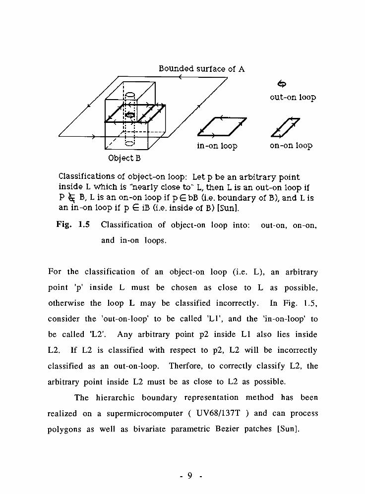
Classifications of object-on loop: Let p be an arbitrary point

inside L which is ""nearly closeto"

L, then L is an out-on loop if

P ^ B, L is an on -on loop if p E bB (i.e. boundary of B), and L is

an in -on loop if p G iB (i.e. inside of B) [Sun].

Fig. 1.5 Classification of object-on loop into: out-on, on-on,

and in-on loops.

For the classification of an object-on loop (i.e. L), an arbitrary

point'p'

inside L must be chosen as close to L as possible,

otherwise the loop L may be classified incorrectly. In Fig. 1.5,

consider the'out-on-loop'

to be called LI', and the'in-on-loop'

to

be called L2'. Any arbitrary point p2 inside LI also lies inside

L2. If L2 is classified with respect to p2, L2 will be incorrectly

classified as an out-on-loop. Therfore, to correctly classify L2, the

arbitrary point inside L2 must be as close to L2 as possible.

The hierarchic boundary representation method has been

realized on a supermicrocomputer ( UV68/137T ) and can process

polygons as well as bivariate parametric Bezier patches [Sun].

- 9

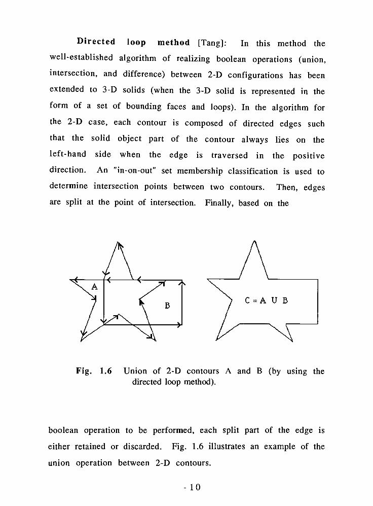
Directed loop method [Tang]: In this method the

well-established algorithm of realizing boolean operations (union,

intersection, and difference) between 2-D configurations has been

extended to 3-D solids (when the 3-D solid is represented in the

form of a set of bounding faces and loops). In the algorithm for

the 2-D case, each contour is composed of directed edges such

that the solid object part of the contour always lies on the

left-hand side when the edge is traversed in the positive

direction. An"in-on-out"

set membership classification is used to

determine intersection points between two contours. Then, edges

are split at the point of intersection. Finally, based on the

Fig. 1.6 Union of 2-D contours A and B (by using the

directed loop method).

boolean operation to be performed, each split part of the edge is

either retained or discarded. Fig. 1.6 illustrates an example of the

union operation between 2-D contours.

- 10

In the 3-D case, contours are replaced with faces. Here

four faces meet at a common edge. The"in-on-out"

classification

of a face is reduced to a 2-D problem by projecting the local

normal vector of each face, (in the neighbourhood of the

intersecting edge), onto a plane perpendicular to the edge. An

example of the 3-D case is illustrated in Fig. 1.7 and Fig. 1.8.

Projection aotit

Fig. 1.7

Example of a 3-D case

(using the directed loop method).

Fig. 1.8

Determination of

the angle between

intersecting faces.

An incoming vector ain is taken as the axis of reference,

the angle included between the outcoming vector aout and ain is

computed.

If ain X aout > 0,

ain X aout < 0,

0 < 0 <180

180

< 0 <360

1 1

Similar calculation is repeated for bin and bout. The normal

vectors are then sorted according to their relative angular

positions. Finally, based on the boolean operation, the relative

angular positions of intersecting faces are compared and each

face is either retained or discarded. This method has been used

in PANDA-3D [Tang]. This method is useful for planar objects but

is inaccurate for curved objects. The authors claim that this

technique is computationally more efficient than the set

membership classification method.

Ray Tracing [Roth]: The ray tracing technique is well

known for rendering highly realistic images. The ray tracing

technique can be implemented at different levels of complexity

depending on the illumination model used with it. For

constructing solid geometric models, a ray tracing technique

called ray casting is used to realize the boolean operations of

union, intersection, and difference.

The observer is assumed to be located along the -fve Z axis.

The view plane (also known as the 'imageplane'

or the 'raster

plane') is the X-Y plane at Z = 0. The models are created in object

space which is the -ve Z half space. All the objects are assumed

to be opaque solids. An object may be either a primitive (such as

a sphere, cylinder, block, or cone) or a composite, i.e. a

combination of primitives. A single point light source is sufficient

to illuminate the object. The light source may be placed by the

user any where in 3-D space.

12 -

In the ray casting process, rays are cast into object space as

probes. A ray originates from the observer's eye, passes through

a pixel on the view plane, and continues into the object space. In

the object space the ray may or may not intersect with the solid

object(s). If the ray does not intersect with any object, the pixel

is displayed with the attributes of the background. The same

process is repeated by casting another ray through the next pixel,

and so on.

Assuming that the ray does intersect with the objects,

intersections of the ray with each primitive component of the

object are determined. From all the intersection points obtained

(for all the primitive components) for a particular ray, one point

is selected depending on the boolean operation being performed

and depending on which object is closest to the view plane. The

algorithm tests to see if the selected point is visible to the

observer or not by examining the angle between the normal at

the selected point and the sight vector. If the point is visible, the

illumination at that point from the light source is determined.

Finally, the pixel on the view plane is displayed with the

attributes (i.e. color) and illumination of the object at the selected

point.

For each primitive at most two ray-primitive intersection

points are determined; the point at which the ray enters the

primitive's surface and the point at which the ray exits the

primitive's surface. Along with the intersection points the normal

at each intersection point is also determined. The surface

13

attributes of the primitive, such as color, are also maintained with

each point. After all the intersection points have been

determined for a particular ray, the list of points is sorted based

on the Z coordinate of the points. From this sorted list, one point

is selected. The criteria for selecting one intersection point based

on the operations of union, intersection, and difference are

explained in section 3.3.2. The ray casting method has been used

in the GM solid modeling project.

When a ray is cast, it is more appropriate to consider it as

being a vector along the line of sight rather than to consider it as

being a reflected light ray (traversed in reverse). After the ray

has entered an object's surface, the ray proceeds through the

object in a straight line along the line of sight without being

refracted. If refraction has to be handled, it must be considered

only after a single intersection point has been selected from all

the intersection points obtained for the ray. Ray tracing of the

refracted ray would then begin from the 'selected point'.

The ray casting method described above can be combined

with either a simple illumination model, a global illumination

model [Rogers], or no illumination at all. The purpose of an

illumination model is to determine the intensity of light reflected

towards the observer's eye at each point on the object's surface.

With the simple illumination model, the ambient light, the

incident light, as well as the light that is reflected diffusely and

specularly from the surface of the object can be considered to

render a model. When the simple illumination model is used, the

14

visibility calculations end at the first ray-object intersection

point. With the global illumination model, it is possible to process

all the effects achieved with the simple illumination model, plus

the following: reflection of one object in the surface of another,

refraction, transparency, and shadow effects. When the global

illumination model is used, the visibility calculations do not end

at the first ray-object intersection point. The reflected ray and

the transmitted ray generated at the intersection point are traced

furthur to determine their intersections with other objects.

Finally, for the case when no illumination model is applied, the

ray casting technique is useful for displaying just the visible

surfaces of a CSG model.

On the whole, a simple illumination model is sufficient to

illuminate an object appropriately. More information about the

simple illumination model is given in chapter 3, section 3.4.

- 15

1.2 REASONS FOR USING RAY TRACING

Among all the methods mentioned in section 1.1, the ray

tracing algorithm for realizing the boolean operations in

constructive solid geometric modeling is, in some sense, the least

complicated and has a wider scope of applicability. Any object

for which an intersection routine can be written may be used for

constructing 3-D models. Objects in a model may be composed of

a mixture of planar polygons, polyhedral volumes, and volumes

defined or bounded by quadric or bipolynomial parametric

surfaces [Rogers]. The boolean set operations, visible surface

processing, and the illumination model, can all be handled

simultaneously by the same algorithm. Illumination of the solids

can be handled at various levels of complexity by using different

illumination equations and techniques. As mentioned in the

previous section, Roth has presented ray casting as the basis for a

CAD/CAM solid modeling system [Roth]. He has also described

how a ray tracing algorithm can be used to generate wireframe

line drawings for solid objects and how it can be used to

determine the physical properties of a solid.

The use of ray casting in a ray tracing algorithm simplifies

determination of ray-object intersection points and the normal

vectors at those points, no matter what orientation, size, or

position the objects may be in. A single ray-primitive

intersection routine is sufficient to process all instances of a

primitive.

Compared to the other methods used for realizing the

16

boolean operations, in the ray tracing method memory usage is

fairly low. Memory usage is directly proportional to the

complexity of a model.

A drawback to using ray tracing is that the algorithm is

slower than many other algorithms when implemented in a single

processor environment. However, the ray-object intersection

calculations can be processed in parallel. Therefore, a ray tracing

algorithm can take advantage of a multiprocessor environment

and speed up the ray tracing process considerably. As

multiprocessor environments become more common, ray tracing

algorithms such as the one proposed become more appropriate

for constructive solid modeling implementations.

17 -

1 . 3 PROBLEM STATEMENT

As mentioned in section 1.1, two main problems in

constructive solid geometric modeling are the representation of

geometric objects, and the implementation of the boolean

operations [Sun]. Most algorithms for performing the boolean

operations are complicated, slow, and of limited applicability

[Tokieda]. Few algorithms have the ability to construct models

using solids that have curved surfaces. Functions such as hidden

line/surface removal, and illumination of the model, have to be

performed by separate algorithms.

In this thesis, a ray tracing algorithm was used to realize

the boolean set operations (The reasons for using ray tracing are

given in section 1.2). A graphics relational database was

designed to facilitate the creation of more complex 3-D solid

models and the storage, manipulation, and deletion of these

models. For displaying a model, a choice was provided between

wireframes for fast display, and shading for displaying a more

realistic object. Shading was done by using a simple illumination

model in combination with dithering.

The software implemented for this thesis has been named

ARTISAN. Software programming was done using the C language.

Software development was done on an IBM AT compatible PC

using a VGA graphics card and a color graphics monitor.

Assembly language routines for using the VGA graphics card

were obtained from the "Programmer's Guide To TheEGA/VGA"

[Sutty].

18

CHAPTER 2 HISTORICAL BACKGROUND

Evolution of the techniques of solid modeling, ray tracing and

dithering are presented below.

2.1 SOLID MODELING

The evolutionary approaches to 3-D object representation are

illustrated in Fig. 2.1 [Voelcker]. Interactive computer graphics

came into prominence in the decade 1955-64. Interactive computer

graphics [Newman] along with projective geometry [Tech.] [Ahuja]

and Numerical Control (NC) programming languages [ITT] gave rise

to the four independent areas of development: polygonal schemes,

sculptured surfaces, wireframes, and solid modeling.

Polygonal Schemes: 3-D modeling systems using polygonal

schemes are mainly used for creating visual effects, i.e. for

rendering. There is a wide range of systems in this field [Newman].

On one end the emphasis is on achieving highly realistic static image

synthesis, while at the other end are real-time animation systems

such as flight simulators.

Sculptured Surfaces: This area deals with mathematical

methods for defining and representing curves and surfaces. The

work of Coons, Bezier, Gordon, and other pioneers dealt with

methods for designing multicurved objects such as ships, car bodies,

aircrafts, etc. The emphasis in this field has been on: accurate

representation of surfaces, and tailoring of such representations to

meet functional and esthetic criteria [Coons] [Bezier] [Forrest]

[Gordon].

- 19

1955

1964

1965

1972

1973

1976

1979

1964

1965

1995

Interactive Computer

Graphics"invented"

I

Homogeneous-coord .

(projective)

geometry

Numerical Control (NC)

programming

languages

VIREFRAMES POLYGONAL

SCHEMES

SCULPTURED

SURFACES

SOLID MODELING

2D systems based Early hidden-line Aero, Auto, Marine Ad Hoc experiments

on drafting prin

ciples; Early NC

from graphic

data bases

andvisible-

surface algo

rithms for

polygonal faces;Simulators

lofting; Parametric

polynominal and

rational curves;

Coons patches;

Bezier surfaces

using diverse

approaches

3D systems;

Better NC;More

conveniences

Bounded

surfaces;

packages;

Color;More

conveniences

Better algorithms

Polyhedral smoo

thing; Faster

simulators; 3D

animation

NC contour milling

from lofted/

digitized surfaces;

B-spline curves

and surfaces

Special computer

hardware;Improved displays;Animation

languages

B-spline

subdivision

algorithms

Experimental boundary ,

CSG, and sweep based

systems demonstrated;Theoretical foundations

emerge

Development of

industrial prototypes;

Early production

versions

T

A narrower spectrum of more powerful systems

Fig. 2.1 A historical summary of approaches to 3-D object

representation (From [Voelcker] page 10).

Wireframes: The wireframe modeling systems first

appeared as 2-D interactive systems. In 1970's they evolved into

3-D systems. 3-D wireframe systems have several drawbacks.

Two serious deficiencies are: (1) they are often ambiguous. Fig.

2.2 illustrates how a wireframe of a cube may represent more

than one solid. This is known as the Necker cube illusion

[VanDam].

(a) (b) (c)

/

Fig. 2.2 The Necker cube illusion. The cube in (a) can be viewed

as the cube in (b) or the cube in (c).

(Necker observed this in 1832).

(2) the viewpoint dependent profile lines that an object with a

curved surface requires in its wireframe are often missing. In

Fig. 2.3, the dashed lines show the profile lines that are often

missing in a wireframe.

Fig. 2.3 Wireframe edges (solid), and viewpoint dependent

profile lines (dashed).

21 -

To overcome these drawbacks, bounded-surface techniques were

used. These in turn led to the use of boundary representation

schemes in some solid modeling systems.

Solid Modeling: This area emerged in the 1960's

[Roberts]. At that time it had very little theoretical support. In

the early 1970's many ad hoc theories were devised to overcome

the need for adequate theoretical foundation. The first

generation of experimental solid modeling systems were

developed in the 1970's. Fig. 2.4 illustrates examples of SM

projects that emerged in the mid 1970's. Theoretical foundations

based on mathematics emerged in late 1970's [Tilove].

1976 CAM- 1 organized its Geometric Modeling Project [Ok ino 1 ] [Ok ino2 ]

MDS I launched i ts Design Project IHakalal [Hillyardl.

1977 General Motors began the development of GMSo I id [Boyse2] .

1978 ShapeData's Romulus system appeared [Ueenmanl.

1979 Two collaborative un i vers i ty/ industry projects were launched:

PflDL-2 at University of Rochester [Brown], and the

Geometric Modeling Project at Leeds in the UK.

1980 Evans fc Sutherland began to market Robu I us.

1981 flppl icon announced a sol id-model ing capabi I i ty based on

SynthaUision [Nagel 1 [Goldstein];

ComputerUision announced the Sol i design system.

Fig. 2.4 Examples of projects that emerged in the mid 1970's

(From [Voelcker] page 13).

22

In the 1980's a second generation of systems were developed.

These were designed for industrial and commercial use. Fig. 2.5

illustrates examples of contemporary CAD/CAM systems.

1988 RDROS (Advanced Design Result Oriented System) developed

in Mexico, [Si ska] .

S I nflK developed in USSR, [Klimovl.

tlODEL developed in Spain at CEIT, [Rodill.

PER I S deve I oped in China in Zhejiang University, [Liang].

Fig. 2.5 Examples of contemporary CAD/CAM systems.

Requicha and Voelcker describe solid modeling as follows [Voelcker]:

"The term "solidmodeling"

encompasses an emerging

body of theory, techniques, and systems focused on

"informationallycomplete"

representations of solids

- representations that permit (at least in principle)

any well defined geometrical property of any

represented object to be calculatedautomatically."

Fig. 2.6 illustrates a generic "geometry system", [Voelcker]. This

may be considered a depiction of the description of SM given

earlier. A typical geometry system has a subsystem called

"geometric modelingsystem"

which accepts definitions of objects

from users and translates them into internal representations.

The subsystem provides facilities for entering, storing, and

modifying object representations.

- 23 -

The subsystem is an independant component and it can be

combined with a variety of applications. The software

implementation for this thesis is an example of the "subsystem".

The command translator accepts questions from the users and

DEFINITIONS OF GEOMETRIC MODELING SYSTEM

OBJECT GEOMETRY f <A SUBSYSTEM)

DEFINITION

XLATOR

I !

Geometric

Models

(Representations)

J_PROCEDURE

~S>4REP

WPROCEDURE

COMMAND

XLATOR

> I REP

^

Vi

Ei

Vi

w

GEOMETRY QUESTIONS (COMMANDS)

Fig. 2.6 A Geometry System. (From [Voelcker] page 10)

evokes application dependent procedures to answer these

questions. For example, questions about the object's volume,

surface area, center of gravity, etc.

Several methods for representation of solids are known

[Requicha] [Mortenson]. Mortenson classified six methods as:

Primitive instancing and/or parametrized shapes, cell

decomposition (along with spatial enumeration), wireframe

representations, sweep representations, boundary

representations, and constructive solid geometry (CSG). Of these

six the last three are used in contemporary SM systems.

24

In primitive instancing [Requicha] each member of a

group of objects is distinguishable by a few parameters, for

example, the family of spike wheels may be described by a type

code, the wheel's diameter and the number of spikes. Primitive

instancing does not allow creation of new or more complex

objects by combining representations. It is also difficult or

impossible to determine geometric properties directly from

primitive instancing schemes.

Spatial enumeration [Requicha] is a scheme where the

occupied space is divided into a 3-D grid of volume elements. A

solid is represented by a list of grid blocks that it occupies. This

scheme has advantages for performing boolean operations,

hidden surface removal or interference detection. However, this

representation is difficult to integrate with database techniques

[Meier]. Thus this scheme is not used in geometry systems as a

fundamental SM method.

The cell decomposition [Requicha] method is based on

the triangulation theory. A solid is decomposed into disjoint

parts of different dimensions. This may be considered a type of

spatial enumeration where cells do not have to lie on a fixed grid

nor have a prespecified size and shape. Like spatial enumeration

this scheme is also difficult to integrate with database techniques

[Meier].

Boundary representation (B-rep) scheme represents a

solid in terms of its boundary. The boundary is viewed as a

closed surface or skin around a solid such that it separates the

inside from the outside. Fig 2.7 illustrates an example of a B-rep

25 -

scheme. The boundaries are represented as unions of faces. Each

face is a union of its edges and each edge in turn is bounded by a

pair of vertices. Accurate boundary representations are difficult

to construct as discontinuity may arise at the juncture of two

surfaces. This method is used in combination with other methods

in contemporary SM systems.

In the sweep representations method, a solid is first

represented by a 2-D plot of its cross section which is called an

"areaset"

[Voelcker] or a"generatrix"

[Siska]. Then another 2-D

plot of the path called the "trajectoryset"

or the"rail"

is

described. Interaction between the generatrix and the running

rail may be carried out in a parallel, radial, or normal (i.e.

perpendicular) way. Using all of this information, the system

generates an isometric view of the solid. This method together

with other methods has been used in ADROS [Siska]. Fig. 2.8,

illustrates some examples of sweep techniques.

CSG and the other SM methods in their embryonic stages

of development recognized the importance of boolean operations.

(For the CSG method see: chapter 1, Fig. 1.1, Fig. 1.2; and chapter

3, section 3.3.2).

26

a

zi'i-i

U = Union of all the faces

Fig. 2.7 A boundary representation. ( From [Voelcker] )

PARALLEL

RADIAL

Rail

k ^K^*v

NORMAL ^&>r X

Generatrix

S X

Fig. 2.6 Parallel, radial, and normal sweep representations.

( From [Siska] )

2.2 RAY TRACING

Ray tracing was first described by Appel in 1967-68,

[Appel]. Initially in the MAGI (Mathematics Applications Group,

Inc.) implementation, the algorithm was used for visible surface

processing of opaque surfaces only, [Nagel]. To make shaded

pictures of solids, the photographic process is simulated in

reverse. The observer is assumed to be on the positive Z axis.

For each pixel in the screen, a light ray is cast from the observer,

through the pixel, into the object space to identify the visible

surface of the object. The first surface intersected by the ray is

the visible one. The surface normal at the ray-surface

intersection point is computed and, knowing the coordinates of

the light source, the brightness of the pixel in the screen is

computed.

This algorithm was later improved so that global

illumination effects such as reflections, refractions, transparency

and shadows could be achieved naturally without implementing

complicated algorithms, [Kay] and [Whitted]. The algorithm used

by most ray tracing programs is described by Whitted. Roth

presented ray tracing as the basic method for a solid modeling

system [Roth]. The research reported by Roth, "Ray Casting for

Modeling Solids", was conducted at the Computer Science

Department of the GM Research Laboratories. This research was

used in the GMSolid modeling project which was developed in

1977-78 for internal use at General Motors [Boyse].

Recently, ray tracing has been used for rendering

- 29 -

parametric patches [Kajiya2] and algebraic surfaces [Hanrahan].

Cook, Porter, and Carpenter have presented a technique of

distributed ray tracing which further enhances realism [Cook]. A

new two-way ray tracing technique has been used in PERIS to

enhance realism [Liang]. In this technique there are two phases.

The first phase is a view-independent process in which rays

emitted from the light source are traced. The second phase is a

view-dependent process in which rays that originate from the

eye are traced.

Since ray tracing consumes a large amount of computer

time, most people are discouraged from using this otherwise

powerful technique. Much work has been done to speed up the

image generation process. Roth has described a screen-space

solution in which minimum bounding boxes are used around the

solids in the CSG composition tree. If it is determined that the

ray does not intersect the bounding box, it is unnecessary to

traverse recursively down the composite's subtrees. Ullner has

described hardware solutions that involve multiple

microprocessors in various configurations [Ullner]. Each processor

manages either a subset of rays or a subset of objects.

The screen-space and hardware solutions, do not

completely solve the problem of slow speed in the image

generation process. Kajiya has shown that doubling the number

of objects in a scene almost doubles the rendering time. Doubling

both the objects and the rays takes four times longer to render

the image [Kajiyal]. To overcome this problem, Glassner

presented a new method in which the number of ray-object

- 30 -

intersections (that must be made to fully trace a given ray) is

considerably reduced [Glassnerl]. In this method the octree

technique is used to dynamically subdivide 3-D space into cubes,

called voxels, of decreasing volume until each cube/voxel

containes less than a maximum number of objects. Each cell of

the octree holds a list of objects that have a piece of their surface

in that cell. In this method, all the voxels in an octree do not

need to be processed. The intersection of a ray is tested for only

those objects that have a piece of their surface in the voxel being

processed. This method reduces the number of ray-object

intersections to a large extent.

In addition to its use for rendering and solid modeling, ray

tracing can be used in animation. Glassner recently presented a

technique for ray tracing animated scenes using spacetime ray

tracing [Glassner2]. He has shown that it is possible to ray trace

large animations much faster with spacetime ray tracing using

hierarchies of bounding volumes, than with the usual

frame-by-frame rendering.

31

2.3 DITHERING

Dithering has been derived from halftoning (also known as

gray scaling). The halftoning technique uses a minimum number

of intensity levels, usually black and white, for increasing visual

resolution [Rogers] [VanDam]. Visual resolution, which is also

known as intensity resolution, is used for making the fine details

in a picture more visible. Originally the halftoning technique was

used in the weaving of silk pictures and textiles. Modern

halftone printing was invented by Stephen Hargon in 1880

[Rogers]. Halftone printing is a screen or cellular process in which

cells can be of variable sizes. Screens with 50 to 90 dots per inch

are used for newspaper photographs. Screens with 100 to 300

dots per inch are used in books and magazines.

In computer generated images a technique called

patterning has been used to increase visual resolution. In

patterning, fixed size cells are used. A pattern

0 1

HFig. 2.9 2 x 2 bilevel pattern cells (From [Rogers] page 102).

cell is formed by combining several pixels. Fig. 2.9 illustrates

patterning using four pixels for each cell. The figure shows five

possible intensity levels. For a bilevel display the number of

possible intensities is one more than the number of pixels in a

- 32

is a tradeoff between spatial resolution and visual resolution.

Spatial resolution is the spatial integration that our eyes perform.

In [VanDam] it has been explained as follows:

"If we view a very small area (say a 0.02 x 0.02 inch square)

from a normal viewing distance, the eye will integrate fine

detail within the small area and record only the overall

intensity of thearea."

The tradeoff between spatial and visual resolution is illustrated in

Fig. 2.10.

When a smaller cell size is used, intensity

(i.e. visual) resolution decreases and spatial

resolution increases. Increase in spatial

resolution can result in contouring.

Contouring occurs when transitions between

adjacent intensity levels become conspicuous.

As the cell size increases, more intensity levels

become available and spatial resolution

decreases. Here there is a balance between

intensity resolution and spatial resolution.

Transitions between intensity levels are more

gradual.

Excess intensity resolution causes a loss of

spatial resolution. Loss of spatial resolution

makes it difficult for the eyes to record the

overall intensity of a small area of the image.

Transitions between adjacent intensity levels

almost disappear.

(a)

(c)

%

Fig. 2.10 Tradeoff between spatial resolution and intensity

(i.e. visual) resolution in patterning.

33 -

Visual resolution can be increased by increasing the cell size but

that results in the loss of spatial resolution. On the other hand,

increase of spatial resolution can result in contouring. To

overcome this, new methods were developed which maintained

spatial resolution while visual resolution was improved.

In the new methods, a fixed threshold was used for each

pixel. If the image intensity was more than the threshold value,

the pixel was white, otherwise it was black. In a simple

thresholding technique, a relatively large amount of error was

generated which resulted in loss of a lot of fine detail in the

image. Floyd and Steinberg developed a technique which

distributed the error to surrounding pixels [Rogers]. The error

was added to the image intensity of each pixel"after"

comparison

with the selected threshold value.

Dithering was another improvement of the thresholding

techinque. In dithering, a random error was added to the image

intensity of each pixel"before"

comparison with the threshold

value. Bayer in 1973 [Rogers] developed an optimum additive

error pattern which was added to the image in a repeating

checker board pattern. This method was known as ordered

dither.

The smallest optimum 2x2 matrix, given below, was

developed by Limb around 1969 [Rogers].

[D2] = [02]

[3 1]

34

Larger ordered dither patterns were obtained recursively by

using the following:

[Dn] = [ 4Dn/2 4Dn/2+2Un/2 ]

[ 4Dn/2 + 3Un/2 4Dn/2 + Un/2 ]

where, n >= 4, and represents the matrix size; and

[Un] = [1 1 ... 1 ] = Unity matrix

| 1 1 ... 1 |I I| I

[1 1 ... 1 ]

2

(n) intensities can be produced from a dither matrix Dn.

The Floyd-Steinberg algorithm, ordered dither, and patterning

techniques can be used with color. (The dither algorithm is

explained briefly in section 3.4 and in [VanDam] on page 601).

35 -

CHAPTER 3 IMPLEMENTATION DETAILS

The software implemented for this thesis has been named

ARTISAN. The major components of ARTISAN are:

(1) The relational database;

(2) The graphic application functions;

(3) The ray tracing algorithm that performs addition,

subtraction, and intersection to build models;

(4) The simple illumination model; and

(5) The graphics display program.

The first four components work together to realize the concept of

constructive solid geometric (CSG) modeling. The relational

database was specially designed and implemented for ARTISAN.

In the second and third components, the techniques used are

similar to the ray casting method used by Roth [Roth]. The fourth

component was incorporated within the ray tracing algorithm and

deals mainly with shading the models. The overall function of

the first four components is to do all the required calculations

and generate display data. The combination of the first four

components is called "Build", and may be referred to as the

"calculations program".

The fifth component, called "Paint", is a separate program

that uses graphics display routines to display models. The

graphics display (GD) program uses the display data generated by

the calculations program. Since the fifth component uses machine

dependent display routines, it is not a portable component. There

are several advantages to separating the calculation and image

-36

display functions into separate programs:

- Each program can be run separately so that MS-DOS

systems with limited memory can be utilized.

The calculation program does not use any system and

machine dependant functions therefore it can be easily

ported to any environment that supports the C

language.

Generation of display data can be done on inexpensive

systems, (i.e. systems that do not have expensive

display hardware and software). The display data

generated can be used by a display program on the

target display machine.

37

3 . 1 THE RELATIONAL DATABASE

The relational database uses three types of relations (a

relation is a group or class of similar objects). The three types of

relations are described below.

(1) Type I relations: In the database, the primitives (i.e.

geometric solids) which have the same characteristics are

grouped into one relation. For example, all instances of spherical

objects are classified as the primitive-type"sphere"

and are

stored in the relation called SPHERE. All instances of cylindrical

objects are classified as the primitive-type"cylinder"

and are

stored in the relation called CYLINDER.

(2) Type II relation: All the models (i.e. composites)

are stored in the relation called MODEL. The MODEL relation is

different from the relations for the primitives. The MODEL

relation is used for storing and manipulating the nonterminal

nodes of the CSG tree in the database, whereas, the relations for

primitives are used for storing the terminal nodes (or leaves) of

the CSG tree.

(3) Type III relation: All the transformation factors

for transforming models (i.e. composites) are stored in the

relation called XFORMS.

Each relation has a DATA file and an INDEX file. Fig. 3.1 (a)

and (b) illustrate datafile records for type I relations: sphere and

cylinder. In Fig. 3.1, the NAME field is the key field (i.e. the name

of a primitive is used to distinguish one primitive instance from

another). The fields CX, CY, and CZ are the x, y, and z coordinates

38

of the center of the primitive. The field RAD is the radius. The

fields HT and DEP hold information about the height and depth of

the primitive. The ORDER field holds the order in which the

object is rotated about the X, Y, and Z axes. The fields RX, RY, and

RZ are the angles of rotation about the x, y, and z axes

respectively. For example, if the value in ORDER is "ZXY", it means

that the primitive is first rotated about the Z axis by the angle RZ,

then it is rotated about the X axis by the angle RX, and finally it is

rotated about the Y axis by the angle RY. The field CAPPED is a

flag that is true when the cylinder has both the top and bottom

lids closed, otherwise the flag is false. Currently the cylinder

cannot be capped at just one end. The USAGE field is a counter

which gives the number of times an object has been used as a

part in one or more models that exist in the database.

Name Cx cy Cz Rad Ht Dep Order Rx Ry Rz Color Usage

(a) Template of a record in the datafile SPHERE.DTA

Name Cx cy Cz Rad Ht Dep Order Rxl*y Rz Color Capped Usage

(b) Template of a record in the datafile CYLINDER.DTA

Fig. 3.1 Datafile records for the primitives: sphere and cylinder.

39

The domain of the NAME field is"character"

strings which

can be up to thirty characters long. The fields COLOR, CAPPED, and

USAGE hold"integer"

values. The ORDER field is a character string,

three characters long. The data values in the rest of the fields are

of type "double".

The USAGE field is significant for the DELETE RECORD

function. When the usage is greater than one, the value (usage 1)

is the number of times that object has been used as a part in

models. An object is deletable, if the object is not a part of any

model, or if the object is a part of a model which has recently been

deleted. Whenever an object is deleted, its usage is decremented

by one. When the usage is equal to zero, it means that the object

has been marked "deleted". The record marked deleted is

physically removed from the data file later on. When usage is

equal to one, it means that the object exists in the database but is

not part of any model, and can be deleted if the user wants to do

so.

Associated with each DATA file is an INDEX file. The

purpose of the index file is to provide fast search and retrieval of

data and to maintain the records in a sorted order at all times. The

records in the index file represent a binary sequence tree

[McFadden]. In a binary sequence tree, the left branch of an

element (i.e. node) leads to elements with key values less than the

key for the given element, and the right branch leads to elements

with key values greater than the given element. In this document

the binary sequence tree is referred to as the index tree. The key

of the first record that is entered in the data file is used to form

40-

the root of the index tree. Fig. 3.2 is a template of an index record.

LEFT FILE

TYPE

LEFT BYTE

OFFSET

KEY

(NAME)

RIGHT FILE

TYPE

RIGHT BYTE

OFFSET

Fig. 3.2 Template of an index record in an index file.

The object's name is stored in the KEY field. The name in the KEY

field can be a"character"

string not more than thirty characters

long. All the rest of the fields hold"integer"

values. The file type

and byte offset together represent the left or right branch of a

node.

The LEFT FILE TYPE can be either"data"

or "index",

whereas, the RIGHT FILE TYPE can be either "data", "index", or

"null". When either of the file types is "index", it means that the

associated byte offset leads to the location of another index

record in the same index file. When the RIGHT FILE TYPE is

"data", the RIGHT BYTE OFFSET is the location of a data record in

the data file. When the RIGHT FILE TYPE is "null", it means that

there are no data records that have a key name greater than the

current key.

The indexing scheme used here is known as dense

indexing. Dense indexing means that the location of a data

record (in the data file) for each index key is directly available

from the index record itself. In indexing schemes that do not use

dense indexing, the data record's location corresponding to an

index key has to be calculated and/or searched. In the scheme

-41

used in this implementation, when the LEFT FILE TYPE is "data",

the LEFT BYTE OFFSET always refers to the location of the data

record for the current key. This type of indexing produces a

skewed tree structure as opposed to a balanced tree structure.

In the type II relation, i.e. in the MODEL relation, each

record represents a non-terminal node of a CSG tree. Fig. 3.3 is

an example of a record in the data file MODEL.DTA. The field

OPERATION is either for, (1) the boolean set operations: union (i.e.

addition), difference (i.e. subtraction), and intersection, or (2) the

transformation of a model. When a model is transformed, the

transformation of the whole model is performed with respect to

the center of any one of its primitive subcomponents. When the

OPERATION is transformation, the LEFT SOLID INFORMATION

leads to the model that is transformed. The RIGHT SOLID

INFORMATION leads to a primitive component (of the model)

with respect to the center of which the model is transformed.

MODEL NAME is the name of the resultant model after

transformation. The transformation factors for translation,

scaling, and rotation of the model are stored in the XFORMS

relation. When the OPERATION is a boolean operation, the LEFT

SOLID represents the first selected object and the RIGHT SOLID

represents the second selected object.

The fields MODEL NAME, SOLID'S NAME, SOLID'S

RELATION, and DATAFILE hold"character"

strings. The

maximum length of the field SOLID'S RELATION can be up to

eight characters. The DATAFILE name can be up to twelve

characters long. The data file name is formed by appending

42-

".DTA"

to the SOLID'S RELATION name. All other strings can be at

most thirty characters long.

MODEL

NAME

OPERATION LEFT SOLID

INFORMATION

RIGHT SOLID

INFORMATION

USAGE

Expansion of LEFT and RIGHT SOLID INFORMATION fields:

SOLID'S

NAME

SOLIDS

RELATION

DATAFILE

NAME

OFFSET

IN FILE

RECORD

LENGTH

Fig. 3.3 Template in the datafile MODEL.DTA.

In the type III relation, i.e. in the XFORMS relation, each

record holds all the information required to transform a

particular model. Fig. 3.4 illustrates a record in the data file

XFORMS.DTA. The field NAME, is the key field. It holds the name

of the resultant model (i.e. the model that results from the

transformation operation). The field OBJ, is the name of the

primitive component with respect to which the transformation is

done. The REL field, is the relation to which the primitive

component belongs (i.e. cylinder, sphere, etc.). The fields DX, DY,

and DZ are the translation factors. The fields SX, SY, and SZ are

the scaling factors. The fields RX, RY, and RZ are the rotation

factors. The fields NAME, OBJ, REL, and ORDER are character

strings (they have the same maximum lengths as mentioned

before). The USAGE field holds"integer"

values. The values in

rest of the fields are of type "double".

-43

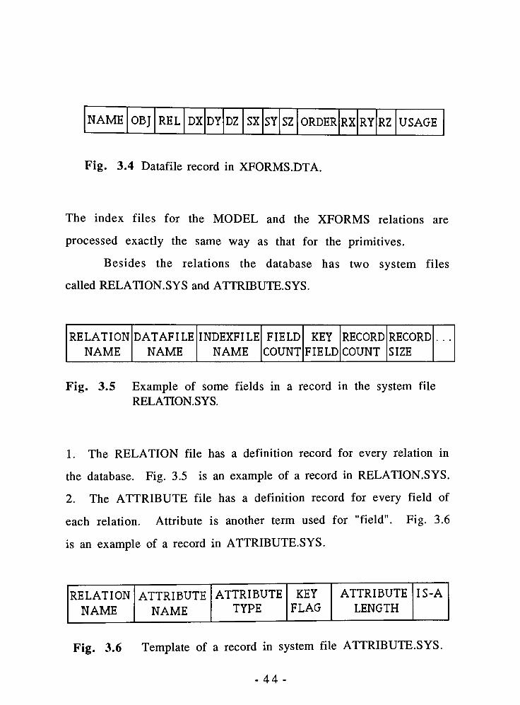
NAME OBJ REL DX DY DZ SX SY SZ ORDER RX RY RZ USAGE

Fig. 3.4 Datafile record in XFORMS.DTA.

The index files for the MODEL and the XFORMS relations are

processed exactly the same way as that for the primitives.

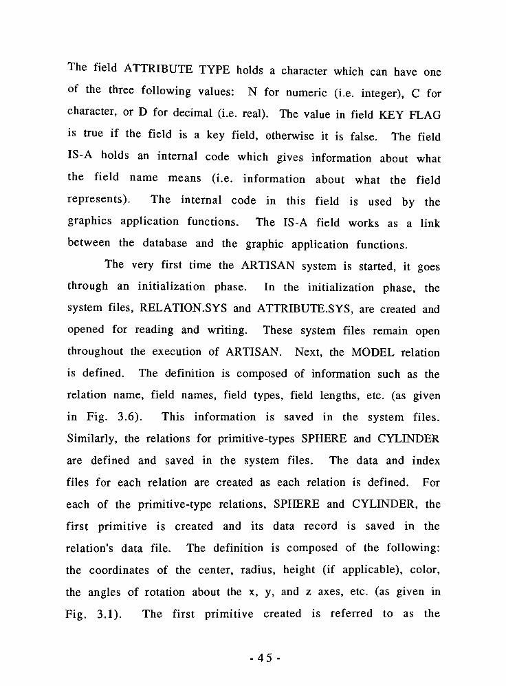
Besides the relations the database has two system files

called RELATION.SYS and ATTRIBUTE.SYS.

RELATION

NAME

DATAFILE

NAME

INDEXFILE

NAME

FIELD

COUNT

KEY

FIELD

RECORD

COUNT

RECORD

SIZE

Fig. 3.5 Example of some fields in a record in the system file

RELATION.SYS.

1. The RELATION file has a definition record for every relation in

the database. Fig. 3.5 is an example of a record in RELATION.SYS.

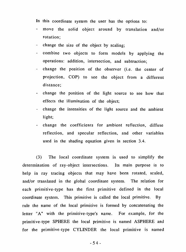
2. The ATTRIBUTE file has a definition record for every field of

each relation. Attribute is another term used for "field". Fig. 3.6

is an example of a record in ATTRIBUTE.SYS.

RELATION

NAME

ATTRIBUTE

NAME

ATTRIBUTE

TYPE

KEY

FLAG

ATTRIBUTE

LENGTH

IS-A

Fig. 3.6 Template of a record in system file ATTRIBUTE.SYS.

44-

The field ATTRIBUTE TYPE holds a character which can have one

of the three following values: N for numeric (i.e. integer), C for

character, or D for decimal (i.e. real). The value in field KEY FLAG

is true if the field is a key field, otherwise it is false. The field

IS-A holds an internal code which gives information about what

the field name means (i.e. information about what the field

represents). The internal code in this field is used by the

graphics application functions. The IS-A field works as a link

between the database and the graphic application functions.

The very first time the ARTISAN system is started, it goes

through an initialization phase. In the initialization phase, the

system files, RELATION.SYS and ATTRIBUTE.SYS, are created and

opened for reading and writing. These system files remain open

throughout the execution of ARTISAN. Next, the MODEL relation

is defined. The definition is composed of information such as the

relation name, field names, field types, field lengths, etc. (as given

in Fig. 3.6). This information is saved in the system files.

Similarly, the relations for primitive-types SPHERE and CYLINDER

are defined and saved in the system files. The data and index

files for each relation are created as each relation is defined. For

each of the primitive-type relations, SPHERE and CYLINDER, the

first primitive is created and its data record is saved in the

relation's data file. The definition is composed of the following:

the coordinates of the center, radius, height (if applicable), color,

the angles of rotation about the x, y, and z axes, etc. (as given in

Fig. 3.1). The first primitive created is referred to as the

45 -

"local/parentprimitive"

(The concept of the local primitive is

explained later in section 3.2). The key (i.e. the name) of the local

primitive is used to create the first index record which is saved in

the relation's index file. The first index record is used as the root

of the index tree.

Currently, the database has definitions and ray-object

intersection routines for the sphere, cylinder, block, and cone.

The definitions and ray-object intersection routines for other

geometric primitives can be installed into the implementation

later. The issues and complexities regarding installation of

definitions and ray-object intersection routines for new primitive

objects are discussed in section 3.6.

46-

3.1.1 USER INTERFACE FUNCTIONS

The relational database is not built on a standard package, it

was specially developed for this system. The relational database

provides user interface through menu driven functions such as:

ADD INTERSECT

BEGIN SESSION MODIFY

CHANGE VARIABLES PRINT TREE

COPY REMOVEDELETEDRECORDS

DELETE SELECT

DELETE ALL SUBSTRACT

DELETECONTENTS TRACEONEOBJECT

DESCRIBE TRANSFORM

DISPLAY

DISPLAY RECORDS

Following is a brief description of the functions:

ADD-

This command is used to perform the boolean operation of

union (+) between the two selected objects. The ray tracing

algorithm is used to realize the boolean operation. The

resultant object is saved in the MODEL relation after the object

has been displayed and approved by the user.

BEGIN SESSION

This command first makes the user select an object by

automatically evoking the SELECT command, then it presents

the user with a second menu of commands. The second menu

47

contains the following commands: SELECT, TRANSFORM, MODIFY,

DELETE, ADD, SUBTRACT, INTERSECT, DISPLAY, COPY, PRINT

TREE, and TRACE ONE OBJECT. All the commands in the second

menu require pre-selection of one or two objects.

CHANGE VARIABLES

This command allows the user to change: the position of the eye

(i.e. the center of projection) along the Z axis, the position of the

point light source, and other illumination variables.

COPY-

This makes a copy of the selected object and saves it under a

new name. In other words this command is used for creating

duplicates of an object.

DELETE -

This command is used to delete the data and index records of a

selected object. The object may be a primitive or a composite.

This command is useful for removing unwanted objects that

may result from commands such as: COPY, TRANSFORM, ADD,

INTERSECT, and SUBTRACT.

DELETE ALL -

The purpose of this command is not only to delete all the

contents of the data and the index files but also to delete the

field definitions from the system's attribute file and the relation

definition from the system's relation file.

48

DELETE CONTENTS -

This is used to delete all the contents of the data and index files

for a specified relation (including the data for the local

primitive).

DESCRIBE

This is used either to display the relation descriptions in the

entire database, or to display the record description of a

particular relation. To describe the database, all the pertinent

information about each relation is displayed. To describe a

particular relation, all the information about the fields of that

relation is displayed.

DISPLAY -

This displays either a wireframe or an illuminated image of the

selected object. The illuminated image is displayed only if

either ADD, SUBTRACT, INTERSECT, or TRACE ONE OBJECT was

the latest command performed.

DISPLAY RECORDS -

This displays all the data records of a specified relation. The

data records are displayed sorted based on the name of the

objects in the relation. After this, the user is provided with an

option to see the index records in the associated index file.

INTERSECT

This command is similar to the ADD command except that it is

49

used to perform the boolean operation of intersection (&)

between the two selected objects.

MODIFY -

This command operates on one selected object. It allows the

user to change the data record of the object. This command

does not result in the creation of a new object. The

TRANSFORM or COPY commands should be used to create new

objects.

PRINT TREE-

This command prints the objects that are present in the CSG

tree of a selected object. It prints the names of the objects and

the relations to which they belong. This command is useful if

the selected object is a model composed of several sub-models

and primitives.

REMOVEDELETED RECORDS -

The purpose of this command is to physically remove data and

index records of objects that have been marked deleted. This

command operates on the data and index files of all the

relations in the database. The data and index files are

re-created for the undeleted objects. Therefore, it is expected

that this command will be used infrequently, i.e. when there are

several records marked deleted as opposed to just one or two.

50

SELECT -

This command is used to retrieve a particular object (primitive

or composite) from the database to perform further functions.

This function builds the CSG tree for the selected object in

memory. Some of the commands that are provided after a

SELECT command are: TRANSFORM, MODIFY, COPY, DELETE

RECORD, TRACE ONE OBJECT, or DISPLAY. These commands are

used to operate on one selected object. (To perform the ADD,

INTERSECT, and SUBTRACT commands, two objects are required,

thus the SELECT command must be used twice to select two

objects before these commands are used).

SUBTRACT

This command is similar to the ADD command except that it is

used to perform the boolean operation of difference (-) between

the two selected objects. The second object is always subtracted

from the first object.

TRACEONE OBJECT -

This command is used to create a solid, shaded image of a

selected object. The boolean operations of union, intersection,

and difference are binary operations which require the

selection of two objects (i.e. components). In order to construct

a complex model, components of the model must be built first.

The components must exist in the database before they can be

combined with other objects. Often it is useful to see what a

sub-component looks like before it is combined with anything

-51-

else. A wireframe of a component just gives a rough idea about

the component's position, size, and orientation but this

command enables the user to see the realistic version of the

component. Thus, this command is used to recreate a solid,

shaded version of any model or primitive that exists in the

database.

TRANSFORM -

This command is used for creating new instances of primitives

or new composites. This command allows the user to translate,

scale, and rotate a selected object. The transformed object is

saved under a new name. Transformation of a composite object

is performed with respect to a user specified primitive

component (of the composite object).

-52

3.2 THE GRAPHIC APPLICATION FUNCTIONS

The graphic application functions, such as: DISPLAY,

TRANSFORM, ADD, SUBTRACT, and INTERSECT, use three kinds of

cartesian coordinate systems:

(1) the screen coordinate system,

(2) the global coordinate system, and

(3) the local coordinate system.

Following is a description of each system.

(1) In the screen coordinate system, the screen (or view

plane) is in the X-Y plane. The plane equation of the view plane is

Z = 0. The 3-D primitives and models are built in the -Z half space

and the eye of the observer is in the +Z half space at (0, 0, Z). The

+Z axis is perpendicular to the screen and points out from the

screen.

For the ray tracing process, a ray originates from the

observer's eye, passes through a pixel on the view plane, and

continues into the -Z half space where the ray may or may not

intersect with the object(s).

(2) The global coordinate system (also known as the scene

or model coordinate system) is the main system the user is aware

of. The user has the option to position the point light source

anywhere in this system. The models are created by the user in

the -Z half space behind the view plane, preferably in the quadrant

defined by the +X, +Y, and -Z axes.

53-

In this coordinate system the user has the options to:

-

move the solid object around by translation and/or

rotation;

-

change the size of the object by scaling;

combine two objects to form models by applying the

operations: addition, intersection, and subtraction;

- change the position of the observer (i.e. the center of

projection, COP) to see the object from a different

distance;

- change the position of the light source to see how that

effects the illumination of the object;

change the intensities of the light source and the ambient

light;

change the coefficients for ambient reflection, diffuse

reflection, and specular reflection, and other variables

used in the shading equation given in section 3.4.

(3) The local coordinate system is used to simplify the

determination of ray-object intersections. Its main purpose is to

help in ray tracing objects that may have been rotated, scaled,

and/or translated in the global coordinate system. The relation for

each primitive-type has the first primitive defined in the local

coordinate system. This primitive is called the local primitive. By

rule the name of the local primitive is formed by concatenating the

letter"A"

with the primitive-type's name. For example, for the

primitive-type SPHERE the local primitive is named ASPHERE and

for the primitive-type CYLINDER the local primitive is named

54

ACYLINDER. Fig. 3.7 illustrates local primitives for the sphere and

the cylinder. The local primitive always has a fixed center, radius,

Y t

l

-S--

c

X

LOCAL SPHERE

-ft*

+ Z

LOCAL CYLINDER

0 = ORIGIN

C = CENTER (1.0, 1.0, -1.0)

RADIUS = 1.0

HEIGHT (OF CENTER) = 1.0

DEPTH (OF CENTER) =1.0

Fig. 3.7 ASPHERE and ACYLINDER, defined in the local coordinate

system.

height (of center), depth (of center), and the angles of rotation

about the three axes. Currently the local primitives for all the

primitive-types are defined as follows:

Center (x, y, z) = (1.0, 1.0, -1.0);

Radius = 1.0;

Height of center =1.0 (Therefore, total height = 2.0 units);

Depth of center =1.0 (Therefore, total depth = 2.0 units);

Order of rotation = "XYZ";

Rotation about x axis, alpha= 0.0;

Rotation about y axis, beta = 0.0; and

Rotation about z axis, gamma= 0.0;

In effect, the local primitive of every primitive-type is used as a

kind of parent primitive from which all other instances of

primitives are derived. The local/parent primitive cannot be

deleted or modified by the user. The local primitive for each

relation is created automatically in the initialization phase when

ARTISAN is started for the first time. When the user first creates

55

a new instance of a primitive, the location, size and orientation of

the new primitive is the same in both, local and global, coordinate

systems. When the user translates, scales, and/or rotates the

new primitive, all the transformations on the new primitive take

place in the global coordinate system only. In the local

coordinate system the new primitive remains constant and

equivalent to the parent primitive.

Whenever the user SELECTS a primitive object, the

transformation factors are determined from the datafile and two

transformation matrices, called LtoM and MtoL, are computed.

These matrices are saved in memory along with other

information about the object. MtoL is a 4 x 4 linear

transformation matrix that transforms the object from the model

(i.e. global) to the local coordinate system. LtoM is a 4 x 4 linear

transformation matrix that transforms the object from the local to

the model coordinate system.

The reason why the local primitive is required for each

primitive-type is because it simplifies the problem of calculating

ray-object intersections during the raytracing process. No matter

what location, size, or orientation the primitive object may have

in the model (i.e. global) coordinate system, a single ray-object

intersection routine (for the local primitive) is sufficient to handle

the raytracing of all the primitive objects of that primitive-type.

The ray-object intersection routine is specially designed to

determine ray-object intersection points for the local primitive.

To raytrace a primitive object the routine uses the object's MtoL

transformation to transform the ray from the model to the local

56

coordinate system. The effect of translating, scaling, and rotating

a solid is achieved by translating, scaling, and rotating the rays

[Roth]. Since, the equation of a ray is the same as the equation of

a line in 3-D space, a ray is transformed by transforming its fixed

point and its direction vector. Consider the ray equation:

rx = cpx + (px -

cpx) T = cpx + aT

ry = cpy + (py -

cpy) T cpy + bT

rz = cpz + (pz -

cpz) T = cpz + cT

Here, rx, ry, and rz are the x, y, and z components of the ray; cpx,

cpy, and cpz are the x, y, and z components of the center of

projection, COP (i.e. the eye); px, py, and pz are the coordinates of

the pixel on the screen; a, b, and c are the x, y, and z components

of the direction vector of the ray; and T is the ray (or line)

parameter. In the given ray equation, the fixed point is the COP

(i.e. cpx, cpy, and cpz) and the ray's direction vector is given by a,

b, and c. The fixed point is transformed as follows:

(cpx', cpy', cpz', 1) = (cpx, cpy, cpz, 1)* MtoL

Where, (cpx', cpy', cpz') is the transformed point. The direction

vector is transformed as follows:

(a', b', c', 0) = (a, b, c, 0)* MtoL

where (a', b', c') is the transformed vector. When the ray is

transformed in this way, the ray parameter T remains constant in

both, local and model, coordinate systems. The equation of the

-57-

transformed ray is obtained as follows:

rx'

=cpx'

+(a' *

T)ry'

=cpy'

+(b' *

T)rz'

=cpz*

+(c' *

T)

Consider a point corresponding to parameter T on a ray in the

model coordinate system. After the ray is transformed to the local

coordinate system, the point (now transformed) still corresponds to

the same T on the transformed ray [Roth]. This implies that

neither the parameters nor the points need to be transformed, only

the ray needs to be transformed between the local and model

coordinate systems.

When the ray is in the local coordinate system, it is not

necessary to find and transform the actual points where the ray

enters and exits the object but it is sufficient to determine the ray

parameters that designate those points.

58

3.3 Ray Tracing Algorithm for Processing a CSG Tree:

Data structures used in this algorithm are given in section 3.3.1.

The criteria for selecting an intersection point are given in section

3.3.2. Input to TraceObject are: a pointer to solid node of binary tree,

the operation, and the ray equation. Output from TraceObject are:

'Xpts'

the intersection point(s), and'Norm'

the normal to each

intersection point.'Xpts'

is an array of type POINTNODE.

TraceObject(SolidNodePtr, Operation, Xpts, Norm) {if (Operation is for a Composite solid) {

TraceObject(L_SolidPtr, ... ); /* These two calls could be

TraceObject(R_SolidPtr, ... ); executed in parallel */

/* Select one ray-object intersection point based on the boolean

operation being performed. */

SeIectXpt(Xpts, ... );

Return;

}

else if (Operation is for a Primitive solid) {

Based on ( PrimitivePtr->Type) {

/* Transform ray to primitive's local coordinate system

using the primitive's MtoL_Xformation.

Determine ray parameters with respect to primitive's

surface equation in its local coordinate system.

Determine if ray intersects with the object at atleast one

point.

If (ray intersects with the object)

Determine outward normal at each intersection point.

Calculate intersection points for the model in object

space (i.e. the global coordinate system) using ray

parameters.

- Save information in: Xpts, and Norm. */

59

3.3.1 DATA STRUCTURES

Following are the minimal data structures that were used for

the CSG tree:

PRIMITIVE NODE: /* leaf node of the CSG tree */

Name-of-primitive

Type /*sphere, cylinder, block, cone, etc. */

LtoM-Xformation /* 4 x 4 transformation matrix */

MtoL-Xformation /* " " "

*/

SOLTDNODE: /*nonterminal/terminal node of the CSG tree */

Name-of-solid

Operation /*+, &, -, or no-operation

*/

L_SolidPtr /*pointer to left solid node

*/

R_SolidPtr /*pointer to right solid node */

PrimitivePtr /*pointer to terminal/primitive node */

When Operation == no-operation, SOLIDNODE represents a

primitive. In this case, the pointers L_SolidPtr and R_SolidPtr are

both NULL. PrimitivePtr leads to the node for the primitive.

When Operation == boolean operation, SOLIDNODE represents

a composite. In this case, the pointer PrimitivePtr is NULL. L_SolidPtr

leads to information of the left solid and R_SolidPtr leads to

information of the right solid.

When Operation == xformation, L_SolidPtr leads to the object

that is to be transformed. R_SolidPtr leads to the reference primitive

with respect to which the object is to be transformed and PrimitivePtr

leads to the transformation factors required to perform the operation.

POINTNODE: /*structure for intersection points and normals */

x, y, z/*

components along x, y, and z axes*/

solidnodePtr/*

pointer for solid through which ray passed */

-60-

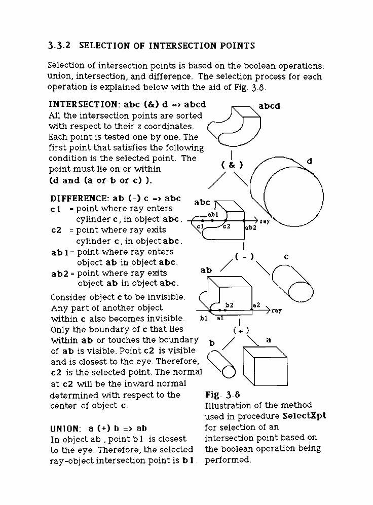
3 3-2 SELECTION OF INTERSECTION POINTS

Selection of intersection points is based on the boolean operations:

union, intersection, and difference. The selection process for each

operation is explained below with the aid of Fig. 3.6.

INTERSECTION: abc (&) d => abed

All the intersection points are sorted

with respect to their z coordinates.

Each point is tested one by one. The

first point that satisfies the followingcondition is the selected point. The

pointmust lie on or within

(d and (a or b or c) ).

DIFFERENCE: ab (-) c => abc

c 1 = point where ray enters

cylinder c,in object abc .

c2 = point where ray exits

cylinder c, in object abc.

ab 1 = point where ray enters

object ab in object abc.

ab2 = point where ray exits

object ab in object abc.

Consider object c to be invisible.

Any part of another object

within c also becomes invisible.

Only the boundary of c that lies

within ab or touches the boundary

of ab is visible. Point c2 is visible

and is closest to the eye. Therefore,

c2 is the selected point. The normal

at c2 will be the inward normal

determined with respect to the

center of object c.

UNION: a (+) b => ab

In object ab ,point b 1 is closest

to the eye. Therefore, the selected

ray-object intersection point is b 1 .performed.

abed

Fig. 3-6

Illustration of the method

used in procedure SelectXpt

for selection of an

intersection point based on

the boolean operation being

The difference operation requires a more in-depth examination of

the intersection points, in contrast to the other two operations. The

possible cases of the difference operation are discussed below.

Consider two objects to be objectl and object2. For the difference (-)

operation it is assumed that object2 is subtracted from objectl.

Consider the following intersection points for the two objects:

enter 1 = point at which ray enters objectl's surface

exitl = exits

enter2 =" " " "

enters object2's surface

exit2 =' "

exits

The outcome of the difference operation between objectl and

object2 can be any of the following cases:

Case 1: If the sequence of ray-object intersection points is either

(enter2 exit2 enter 1 exitl) or (enter 1 enter2 exitl exit2),

the point enterl which belongs to the first object is the

selected point since it is the first visible point in the line of

sight.

Case 2: If the sequence of intersection points is

(enter2 enterl exit2 exitl), object2 lies partially within

objectl. This is the case explained before with the help of

fig 3.8. Point exit2 is the selected point and the normal at that

point is the inward normal determined with respect to the

second object. The color associated with the point is changed

to the color of the first object.

-62

Case 3: If the sequence of points is (enter2 enterl exitl exit2), the

second object passes through the first object such that the

background is visible to the observer. In this case, the point

exit2 is the selected point and its color is changed to the color

of the background.

Case 4: Consider the first object to be a composite solid made up of

two primitives, primitive 1 and primitive3.

enter3 = point at which ray enters primitive3's surface

exit3 ="

exits

The points enterl, exitl, enter3, and exit3 all belong to the

first object as a whole. The points enter2 and exit2 belong to

the second object. If the sequence of points is

(enter2 enterl exitl exit2 enter3 exit3), it implies that

object2 passes through primitivel but lies ahead of

primitive3. Therefore, in this case, primitive3 is visible to the

observer and the selected point is enter3.

To be able to examine all the intersection points obtained with

a ray for the difference operation, arrays called 'Zbuf and'Znorm'

were utilized. 'Zbuf is an array of intersection points of type

POINTNODE and can hold more points than the'Xpts'

array.'Znorm'

is a parallel array that holds the normal at each point in 'Zbuf. In

procedure SelectXpt, first 'Zbuf was sorted based on the

Z-coordinates of the points, then the sequence of points was

examined in the manner explained for the cases given above.

63

3.3.3 BOUNDING VOLUMES

The algorithm in section 3.3 gives an idea of how much time

is consumed in transforming the ray from model to local coordinate

system, determining intersections, selecting an intersection point,

etc. All this time is a waste if the ray clearly misses the solid

object. Therefore, both an object-space and a screen-space solution

[Roth] were used to detect if the ray clearly missed the solid. For

the object-space solution, bounding volumes such as bounding

sphere or bounding box were used. A bounding box (or box

enclosure) is a tight rectangular parallelopiped around the solid in

the model coordinate system. The box for an object was computed

at the time when the user SELECTed the object. The box is defined

by six points: xmin, xmax, ymin, ymax, zmin, and zmax. These

coordinates were saved, along with other information about the

object, in the object's CSG tree in memory. For the screen-space

solution, the projection of the box enclosure on the view plane was

used to detect if a ray missed an object.

During the raytracing process, the pixels on the screen are

usually scanned from left to right and from top to bottom. Before

beginning the raytracing process it is necessary to determine the

area of pixels that should be scanned so that the entire solid in

object space gets ray traced. The area of pixels to be scanned is

determined by using the box enclosures mentioned earlier. Before

the ray tracing process was started, a special procedure recursively

descended the CSG tree from the root node to the leaves. At the

-64-

terminal nodes it determined the 2-D projection of the bounding

box upon the view plane. The projected vertices were saved in an

array called ScanList and were used later for the screen-space

solution in the ray tracing algorithm. As the procedure returned

up the tree, at each node it combined the projected areas of the left

and right subtrees. When the procedure returned to the root node,

it had the whole area to be traced for the entire object. Tracing

started at pixel (xmin, ymax), and ended at pixel (xmax, ymin).

For the screen-space solution, in the ray tracing algorithm, if

it was determined that the pixel (px,py) under consideration did

not lie within the projected area for a particular node, then it was

unnecessary to traverse down the subtrees of that node. For the

object-space solution, after the ray equation was determined, a

ray-box intersection test was performed. If this test failed for a

primitive in the CSG tree, it meant that the ray clearly missed the

primitive and that it was not necessary to perform the

ray-primitive intersection test.

65

3.4 THE ILLUMINATION MODEL

In ARTISAN, the light is assumed to be a single point light

source. All the objects are assumed to be opaque (i.e. non-transparent)

solids having smooth surfaces. The only variable surface attribute for

all primitives is color. The illumination model used in ARTISAN, is

invoked locally. That means, only the light from the light source and

the object's surface orientation are taken into consideration to

determine the intensity of the light reflected to the observer's eye.

This illumination model is also known as the simple illumination

model. The equation used by the simple illumination model to

determine intensity, takes into consideration the ambient light,

incident light, and light reflected diffusely and specularly from the

object's surface. The following equation was used to calculate the

intensity at a point.

I = ia.Ka +

U |"Kd Cos(e) + Ks- Cosset)!

where I = reflected intensity,

la = incident ambient light intensity,

1 1 = incident intensity from a point light source,

Ka = ambient reflection constant (0 ^ Ka ^ 1),

Kd = diffuse reflection constant (0 Kd ^ 1),

Ks = specular reflection constant,

66

K = an arbitrary constant,d = distance from perspective viewpoint to the object,

8 = angle between the light direction and the surface

normal (0^6^ 7t/2 ),-* = angle between the reflected ray and the line of

sight (-71/2 ^ ct z %/2 ), and

n = a power that approximates the spatial

distribution of the specularly reflected light.

This equation can be reduced to the Lambertian diffuse

reflection illumination equation which uses just the intensity of

incident light, the diffuse reflection constant, and cosine of the angle of

incidence. The Lambertian diffuse reflection equation was sufficient

to produce good results. After the reflected intensity was determined,

an ordered dither algorithm was used to determine the final display

value for the pixel. For more information about dithering see section

2.3. In the dither algorithm, position (i, j) in the dither matrix is

determined first.

i= Px MOD n;

j = Py MOD n;

Then, the pixel display value is determined as follows:

if I(Px, Py) < DMAT(i, j) then

Value = 12;

else Value = I(Px,Py);

where MOD is a function that returns the modulo value of its

arguments,

(Px, Py) designate the pixel on the raster (i.e. viewplane),

DMAT is the ordered dither matrix of dimension n x n,

I(Px, Py) is the reflected intensity at the pixel (Px, Py),

Value is the final intensity for the pixel, and

12 is a reflected intensity slightly lower than I(Px,Py).

67 -

3.5 GRAPHICS DISPLAY PROGRAM

The graphics display (GD) program can run on systems that

have a CGA (Color Graphics Adapter), EGA (Enhanced Graphics

Adapter), or VGA (Video Graphics Array) graphics adapter and

display hardware.

In ARTISAN, as the ray tracing algorithm determines and

selects the ray-object intersection points, it writes the following

information to an output file: the coordinates (Px, Py) of the pixel

through which the ray passed, the color of the solid to which the

intersection point belonged, and the intensity at that point. When

the GD program is evoked it simply opens the output file and

displays each pixel with an appropriate shade of a color depending

on the given intensity at each pixel.

Similarly, for displaying a wireframe of a solid object, all the

calculations are done in ARTISAN and the points and lines to be

displayed are written to the output file (along with the color at

each point). The GD program processes the points read from the

output file in the same manner as mentioned above. Different and

small size versions of the GD program can be easily written to

facilitate the presentation of image data on displays supported by

Sun windows, X windows, or any other windowing system or

display technology.

68

3.6 HELPFUL HINTS

Following are a few helpful things to keep in mind while

building a model:

1. If the object that is to be subtracted has the option to be

either capped or open, such as a cylinder or a cone, the

user must make it capped rather than open.

2. Often either one or both components of a model need to be

modified before a boolean operation can be performed on

them. The best way to handle this is to evoke the

operation command ADD, SUBTRACT, or INTERSECT, see

what the combined components look like in a wireframe

display and return to the menu without saving the

combination as a model. The components can be modified

and the above procedure can be repeated until the model

is correct.

3. A complex model should be built with all its components in

a particular orientation. The whole model should be

transformed only after all the components have been

combined together.

4. The size of an object can be changed in two ways. One way

is to use scaling to make an object bigger or smaller. The

other way is to translate the object closer to the view plane

or further away from the view plane. (Due to perspective

projection objects that are closer to the view plane appear

to be larger than objects of the same size that are far away

from the view plane). Changing the position of the

-69-

observer along the +Z axis does not have the same effect on

the size of the object. As the observer moves away from

the view plane the projection of the object on the view

plane becomes parallel in appearance rather than

perspective. As the observer moves toward the viewplane

the projection becomes more and more perspective in

appearance.

5. When an object is created care must be taken to see that it

is completely behind the view plane (unless the user

purposely wants the view plane to cut through the object).

6. The position of the point light source plays an important

role in the shading of the model. Best results were

obtained when the point light source was placed fairly

close to the model (about 100 to 200 units away from the

model).

70

3.7 INSTALLATION OF NEW PRIMITIVE TYPES

Installation of new primitive types into the database cannot

be done interactively by the user. New primitive types have to be

installed into the database by a software programmer. Installation

of new primitive types has no effect on the definitions and routines

for primitives that already exist in the database. For example, the

following steps were taken to install block and cone into the

database. The highlighted items are the new statements that were

added to the existing code.

1. In the file "globals.h", the block and cone definitions were

added as follows:

r In the include file"globals.h"

*/

#define MODEL 10

#define SPHERE 20

#define CYLINDER 30

#define BLOCK 40

#define CONE 50

2. In the file "get_type.c", there are two procedures called

GetObjtype and GetPrmtype. Procedure GetObjtype examines the

given relation name to determine if the object belongs to the

COMPOSITE (i.e. MODEL), PRIMITIVE, or XFORMS relations.

Procedure GetPrmtype examines the given relation name to

determine if the primitive object is a SPHERE, CYLINDER, BLOCK, or

CONE. The statements for block and cone were added to these

procedures as follows:

71

/*

In the source file"get_type.c"

*/

GetObjtype(srelation,solidtype)char srelation[];

int 'solidtype;

{if (strcmp(srelation,"MODEL") == 0)

-solidtype = COMPOSITE;else if (strcmp(srelation,"SPHERE") == 0)

solidtype = PRIMITIVE;

else if (strcmp(srelation,"CYLINDER") == 0)

solidtype = PRIMITIVE;

else if (strcmp(srelation,"BLOCK") == 0)'solidtype = PRIMITIVE;

else if (strcmp(srelation,"CONE") == 0)

'solidtype = PRIMITIVE;

}

/*

In the source file"getjype.c"

*/

GetPrmtype(srelation,prmtype)

char srelation[];

int 'prmtype;

{if (strcmp(srelation,"SPHERE") == 0)

solidtype = SPHERE;

else if (strcmp(srelation,"CYLINDER") == 0)

solidtype = CYLINDER;

else if (strcmp(srelation, "BLOCK") == 0)

?solidtype = BLOCK;

else if (strcmp(srelation,"CONE") == 0)

*solidtype = CONE;

}

72

3. Each field required by a primitive type must have a

predefined field name code. All the field name codes are defined

in a file called"is_a.h"

as follows:

#def

#def

#def

#def

#def

#def

#def

#def

#def

#def

#def

#def

#def

#def

#def

ne

ne

ne

ne

ne

ne

ne

ne

ne

ne

ne

ne

ne

ne

ne

OBJNAME 1

OBJTYPE 2

DX 3

DY 4

DZ 5

SX 6

SY 7

SZ 8

RX g

RY 10

RZ 1 1

COLOR 12

CAPPED 13

USAGE 26

ORDER 27

No new information was added in"is_a.h"

because the field name

codes required to define sphere and cylinder can be used to define

block and cone too.

In the procedure GetList (in the source file "chklist.c"), the

case statements for block and cone were added after the case

statements for sphere and cylinder. The fields that a primitive

type requires were put into an array called"Clist"

(also referred to

as "CheckList"). A primitive type (or relation) can have at most

fifteen fields. Clist/CheckList is a list used by procedure DefineRel

and MakePr.

73

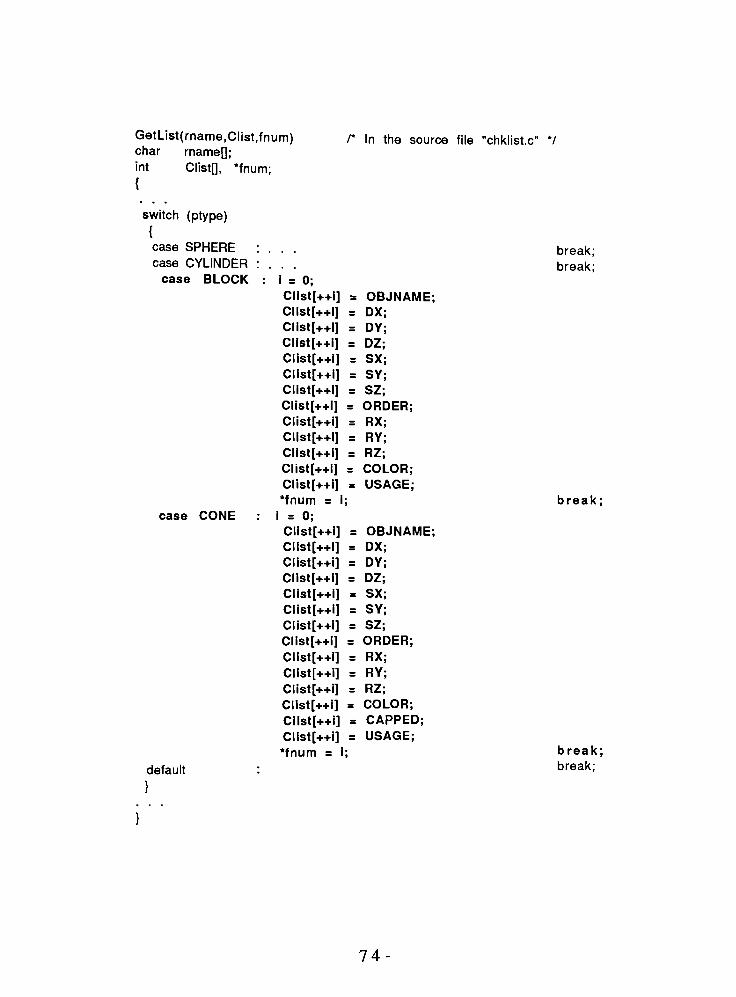
GetList(rname,Clist,fn jm)/*

In the sour

char rnamefj;

int Clistf], *fnum;

{

switch (ptype)

{case SPHERE

case CYLINDER : .

case BLOCK : I = 0;

Clist[++i] = OBJNAME;

Clist[++I] = DX;

Clist[++I] = DY;

Clist[++i] = DZ;

Clist[++i] = SX;

Clist[++1] = SY;

Clist[++i] = SZ;

Clist[++i] = ORDER;

Clist[++i] = RX;

Clist[++i] = RY;

Clist[++i] = RZ;

Clist[++i] = COLOR;

Clist[++i] = USAGE;

*fnum = I;

case CONE I = 0;

Clist[++i] = OBJNAME;

Clist[++i] = DX;

Clist[++i] = DY;

Clist[++i] = DZ;

Clist[++i] = SX;

Clist[++i] = SY;

Clist[++i] = SZ;

Clist[++i] = ORDER;

Clist[++i] = RX;

Clist[++i] = RY;

Clist[++i] = RZ;

Clist[++i] = COLOR;

Clist[++i] = CAPPED;

Clist[++i] = USAGE;

*fnum = i;

break;

break;

break;

default

}

break;

break;

74

DefineRel used CheckList to formulate the definitions of the new

primitive type. The definitons were then saved in the system files:

relation.sys and attribute.sys. Every field in CheckList must have a

case statement for it in the procedure DefineRel. The procedure

DefineRel is in the source file "define_p.c". In the procedure

DefineRel the fields were defined as follows:

DefineRel(relname)/*

In the source file"define_p.c"

*/

char relname[];

{

/*

Creates data and index files. For block the files created are BLOCK.DTA and BLOCK.NDX */

Mk_data_index();

GetList(rname,CheckList,&items);/*

Gets the list of field name codes */

/*

Builds the definition of each field one by one and writes it into the attribute.sys file */

switch (CheckList[a_count])

{I*

NOTE: Each field name code in CheckList must have a case statement here */

case OBJNAME : Scopy(abuffer.aname,"NAME");

abuffer.atype = CHARACTER;

abuffer.alen = NAMELEN;

abuffer.akey = TRUE;

break;

case DX : Scopy(abuffer.aname,"CX");

abuffer.atype = DECIMAL;

abuffer.alen = sizeof(double);

abuffer.akey = FALSE;

case DY : Scopy(abuffer.aname,"CY");

case DZ : Scopy(abuffer.aname,"CZ");

break;

break;

break;

case SX : Scopy(abuffer.aname,"RAD");

abuffer.atype = DECIMAL;

abuffer.alen = sizeof(double);

abuffer.akey= FALSE;

break;

default : . .

break;

/*

Writes definition of the primitive type's relation into the relation.sys file */

75

The definition of each field requires a name, a field type, a field

size, and a key flag. The name is specified so that the user can

understand what the field is. The type can be either CHARACTER

(for text), NUMERIC (for integers), or DECIMAL (for real numbers).

The size is the maximum size the data in a field could have. The

key flag is true for the name field and false for all the other fields.

The procedure MakePr used CheckList to create the first primitive

(i.e. the local primitive) for the new primitive type. (Procedure

MakePr is in the source file "makepr.c"). For the block, MakePr

created the first block called ABLOCK, and for the cone, MakePr

created the first cone called ACONE. Every field in CheckList must

have a case statement for it in the procedure MakePr. MakePr

uses standard data predefined for the local primitive. The local

primitive data is defined in LocalPrm (in the source file "main.c").

LocalPrm is a structure of type PR_BUFFER. For each field there

must be a member (or holder) in the PR_BUFFER structure.

LocalPrm must have a default value initialized for each field.

PR BUFFER and LocalPrm are defined as follows:

76-

typedef struct_prbuffer

{char pname[PNAME];char relation[FNAME];char rname[PNAME];char r_rel[PNAME];

double dx;

double dy;double dz;

double sx;

double sy;

double sz;

double r x ;

double ry;

double rz;

char order[OLEN];

int color;

int capped;

int usage;

} PR_BUFFER;

/*

In the file "structs2.h"

*/

/*

Name of the primitive object *//*

Primitive type: block, cone, etc. *//*

Used for XFORMS: name of object to the right *//*

Used for XFORMS: relation of right object *//*

X-coordinate of object's center *//*

Y-coordinate of object's center *//*

Z-coordinate of object's center *//*

Half of object's width *//*

Half of object's height *//*

Half of object's depth *//*

Angle of rotation about X-axis *//*

Angle of rotation about Y-axis *//*

Angle of rotation about Z-axis *//*

Order of rotation. OLEN = 3 *//*

Color of the object *//*

TRUE if object is capped, FALSE otherwise *//*

Number of times the primitive is used */

/*

LocalPrm is initialized in the file"main.c"

as follows */

PR_BUFFER LocalPrm = {II H fill If II W H

- -

J I

1.0, 1.0, -1.0,

1.0, 1.0, 1.0,

0.0, 0.0, 0.0,

{ 'X', 'Y', 'Z','\0'

},

2, 1, 1

};

4. In the main procedure, procedure calls to DefineRel and

MakePr were added for block and cone as follows:

main( )

{

DefineRel("SPHERE");

MakePrfSPHERE");

DefineRel("CYLINDER");

MakePrfCYLINDER");

DefineRel("BLOCK");

MakePr("BLOCK");

DefineRel("CONE");

MakePr("CONE");

77

5. In procedure MakeTree (in the source file "activates"), if

the flag"capped"

is irrelevant for a primitive type, then the flag

must always be set to TRUE when an object is selected. The

primitives such as sphere and block always have the flag"capped"

set to TRUE. Whereas, primitives that have lid(s), such as cylinder

and cone, may have the flag"capped"

set to TRUE or FALSE.

6. In procedure TraceObject (in the source file "raytrace.c"),

case statements for block and cone were added as follows:

TraceObject(

{

switch (ptype)

{case SPHERE break;

case CYLINDER break;

case BLOCK TraceBlock(. );

> break;

case CONE TraceCone(. . );

default

. . . break;

break;

}

TraceBlock is a routine (in the source file "trcblock.c") that was

implemented to determine ray-block intersections. In TraceBlock,

the interseciton of the ray with each face of the block was tested

one by one. The normal at each point was also determined. The

procedure returned the ray parameters for the points at which the

ray entered the block's surface and the point at which the ray exit

the block's surface. The normal at these points were also returned.

78

TraceCone is a routine (in the source file "trccone.c"), that

was implemented to determine ray-cone intersections. In

TraceCone, mainly two intersection tests were required.

Intersection of the ray with the quadric surface of the cone and

intersection of the ray with the base of the cone were determined.

The procedure returned the ray parameters and normals at the

intersection points.

7. In the procedure DoFrame (in the source file

"wirefram.c"), case statements for the block and cone were added

as follows:

DoFrame()

{

switch (ptype)

{case SPHERE

case CYLINDER

case BLOCK

case CONE

default

SphrFrame( );

CylnFrame( );

BlockFrame( );

ConeFrame( );

break;

break;

break;

break;

break;

}

}

The procedure BlockFrame was implemented to process the wire

frame for blocks. The procedure ConeFrame was implemented to

process the wire frame for cones.

8. All new source files that were created were included in

the"makefile"

to be compiled and linked with the rest of the

implementation.

79

3.8 INSTALLATION OF NEW FIELDS

This section discusses the steps required to install a new

field into a primitive's definition in the database. (Refer to step 3

of section 3.6 for files, procedures, and structures mentioned in the

following explanation).

Consider the hypothetical situation, where a new field for

'transparency'

was to be installed for the primitive type cone. The

new field would function as a flag which would be true if the object

was transparent, and false if the object was opaque.

1 . First, the field name code TRANSP must be defined in the

file, "is_a.h".

2 . In the case statement for cone, in procedure GetList, the

additional field name code TRANSP must be included in the

array Clist.

3 . In procedure DefineRel, an additional case statement must be

inserted for TRANSP. The case statement must specify the field

name to be "TRANSPARENT", the type to be NUMERIC, the field

length to be the size of an integer, and the key flag to be FALSE.

4 . In the structure PR_BUFFER, a new member called"transp"

of

type int must be defined.

5. In LocalPrm a default value (false, i.e. 0) for the new field must

be initialized.

6. In procedure MakePr, a case statement for TRANSP must be

inserted. In the case statement for TRANSP, the default value

80

(for transparency) in LocalPrm must be assigned to the data

structure used for creating the first primitive for cone.

7. In the procedure CopyBuffer, a statement for the new field is

required. In CopyBuffer, contents of the second buffer are

copied to the first buffer. Both buffers are structures of type

PR BUFFER.

CopyBuffer(buf1,buf2)PR_BUFFER *buf1, *buf2;

{

buf1->color = buf2->color;buf1->capped = buf2->capped;

buf1->transp = buf2->transp;

}

8 . In procedure ShowBuf, the value assigned to the field for

transparency must be displayed along with the value assigned

for color, etc.

9 . In procedure Process, first the new transparency option must

be included in the menu for options that the user can change.

Then, a case statement must be inserted for the transparency

option similar to the case statement for the"capped"

option.

10. In procedures CopyPrData and CopyPdata, case statements for

TRANSP must be included. In CopyPrData, contents of a buffer

(of type PR_BUFFER) are copied to another data structure. In

CopyPdata, contents from another data structure are copied to

a buffer (of type PR_BUFFER).

11.Wherever a structure of type PR_BUFFER is used, code

statements to handle the new field must be included.

81

12. The old definition of cone, along with the contents of the data

and index files for cone, can be removed from the database by

using the DELETE ALL command in ARTISAN.

After recompilation and execution of ARTISAN, the new

definition of cone will get installed into the database and the local

primitive called"ACONE"

will be created automatically.

82

CHAPTER 4 CONCLUSIONS

4.1 SUMMARY

The main function of the system implemented is to facilitate

the creation and depiction of non-geometric, complex, realistic,

three dimentional solid models. The system implemented includes

its own graphics relational database which provides a means of

creating, storing, manipulating, modifying, and deleting the 3-D

models. The process of building a 3-D model is based on the

concept of constructive solid geometric modeling (CSG). Geometric

primitives such as a sphere, cylinder, block, and cone are used as

building blocks. The geometric primitives are combined together

by using the boolean operations of union (+), intersection (&), and

difference (-). A ray tracing algorithm is used to realize the

boolean operations. In the ray tracing algorithm, the technique of

ray casting is used to determine the ray-object intersections. A

simple illumination model, using a point light source, is used to

shade the models. The technique of ordered dithering is used in

combination with the simple illumination model to improve the

shading of a model.

The system provides the user with the options to move the

solid model around by translation and/or rotation, change the size

of the model by scaling, change the position of the observer (i.e. the

center of projection, COP) to see the model from a different

distance, change the position of the light source to see how that

effects the illumination of the model, and change the intensity of

the light source and other illumination variables. While creating

83 -

and editing the models the user has the option to view the model

either as a wireframe for fast display or as a shaded solid for a

realistic display.

The ray tracing algorithm handles the boolean set

operations, visible surface processing, and the illumination of the

model simultaneously. Since the ray-object intersection calculations

can be processed in parallel, the ray tracing technique becomes

more appropriate for constructive solid modeling compared with

the other implementation techniques mentioned in section 1.1,

given a multiprocessor environment.

Software implementation was done in the C language, on an

IBM AT compatible PC using a MS-DOS operating system, a VGA

graphics card, a color graphics monitor, and a math co-processor.

The whole implementation, which is known as ARTISAN, is

composed of two programs. One program, "Build", performs the

calculations and generates display data, and the other, "Paint", uses

the data generated to display the image. The calculation program

does not use any system or machine dependent functions, whereas

the graphics display program uses machine dependent display

routines. The calculation program has a menu driven user

interface which may not be as user friendly as a graphical user

interface but it preserves the portability of the program.

The process of building a model that has several

sub-components can be time consuming if the ray tracing

algorithm is used every time two components are combined

together. So the ADD, SUBTRACT, and INTERSECT commands allow

the user to see wireframe representations of the components, and

84

save the resultant model in the database without actually ray

tracing the resultant model. The wireframes give the user a rough

idea about the placement, size, and orientation of the components.

Thus, the time utilized in building a complex model can be greatly

reduced by using the wireframe displays for viewing the progress

of the model building process. Once the entire model has been

built, it can be ray traced.

85

4 . 2 SOLUTIONS TO PROBLEMS ENCOUNTERED

1) Internal meaning: In order for the graphic application

functions to interpret the fields in a record, an extra field

called IS-A was added to each field's definition, in the

system file ATTRIBUTE.SYS. For example, for the application

functions, internally the LENGTH of a block means the same

as twice the RADIUS of a sphere. Both LENGTH and RADIUS

give information about the dimensions of the objects along

the x-axis. Thus, both LENGTH and RADIUS have identical

IS-A fields. Another use of IS-A is that it makes the field's

meaning independent of the field's position in the record.

That means, the position of a field could be first, last, or

anywhere in between in a record. Without the IS-A field, it

would be harder for the application functions to interpret

information in the database.

2) Deletion of a subcomponent: For the function DELETE

RECORD, an object could not be deleted and physically

removed from the database if the object was being used as a

part of other solid models. This problem could be solved by

adding a field called PART-OF to each object's record. The

information in PART-OF would lead to a list of models of

which the object is a part. Instead of using this scheme a

simpler method was used. Instead of PART-OF, a field called

USAGE was used with each object's definition. USAGE holds

the number of times the object has been used as a part of

other models in the database. When a model (i.e. composite)

86 -

is deleted, the USAGE of its subcomponents (i.e. submodels

and primitives) is decremented by one. When a model is

created, the USAGE of its subcomponents is incremented by

one. More information about the USAGE field is given in

section 3.1.

87

4 . 3 DEFICIENCIES

1 ) Currently ARTISAN has definitions and ray-object

intersection routines for the primitive types cylinder,

sphere, block and cone. Installation of new primitive

types, such as the torus, into the database cannot be done

directly by the user. Installation of new primitive types

can be done only by a software programmer, as explained

in section 3.6.

2 ) The display data that results from the ray tracing

algorithm or the wireframe function is stored in the output

file, called "outfile". This output file is then used by the

graphics display program to display the image. Output

files are often quite large, therefore to conserve disk

storage the software currently reuses a single data file to

store display data. By reusing the output file its previous

contents are lost. If it is required that the display data for

a particular session be saved, the user must manually copy

the data file to a file with a different name.

3 ) The simple illumination model, discussed in section 3.4,

does not take into consideration the light that reaches an

object's surface by reflection from, or transmission

through, other objects. The simple illumination model does

not process shadows. To incorporate these illumination

88

effects, a global illumination model would be required. A

brief description of a global illumination model is given,

along with an explanation of the ray tracing technique, in

section 1.1. In a global illumination model shadows are

processed by default. A global illumination model is

computationally more expensive than a simple illumination

model. For more information about the global illumination

model refer to [Rogers].

4 . 4 FUTURE EXTENSIONS

1 ) Currently ARTISAN has a single point light source which

the user may place anywhere in 3-D space. Additional

light sources could be added to improve quality of images.

For multiple light sources, the illumination effects get

added linearly. The shading function given in section 3.4,

for calculating the reflected intensity becomes:

l ._ ia.Ka +fJ^[Kd.Cos<6-) -

Ks.CosJ<*.)]i = i

The additional light source(s) would first be defined in the

file "constant.h", similar to the point light source already

defined. In the procedure ChangeLight, the user is given

89

an option to change the position of the light source. Code

statements could be inserted in procedure ChangeLight to

give the user options to change the additional light

source(s). Then, in the procedure Shade (in the source file

"shadec.c"), the angle of incidence (i.e. the angle between

the surface normal and the light vector), would have to be

tested for each light source. Those light sources for which

the angle of incidence is not in the range of0

to 90, must

be ignored. The other valid light sources would have to be

taken into consideration. In the procedures Shade (in the

source file "shadec.c") and Dither (in the source file

"dither.c"), the reflected intensity would have to be

calculated (using the equation given above) for each valid

light source.

2 ) ARTISAN assumes that all objects are opaque and have

smooth surfaces. However, objects could have the option to

be transparent. It is possible to process objects that have a

semitransparent, nonrefractive surface, by using the

simple illumination model. If the first object that a ray

intersects is transparent, it implies that:

- both the outer and inner surfaces of the first

object are visible to the observer, and

-

any objects that lie behind the first object are

also visible to the observer.

Therefore, for the first object, all the ray-object

- 90

intersection points are tested for visibility using the

outward surface normal as well as the inward surface

normal. All visible points are taken into consideration.

The objects that lie behind the transparent object are

processed the same way depending on whether they are

opaque or transparent. To process refractive transparent

objects, implementation of the global illumination model

would be more appropriate. For more information on

transparency see [Rogers].

If objects had the option to be transparent, a new

field would have to be installed in the primitive's

definition in the database. The procedure for installing a

new field in the primitive's definition is given in section

3.7.

3 ) When a global illumination model is implemented, shadow

effects get processed automatically. However, a special

procedure to process shadows could be added to the simple

illumination model. The test to see if an intersection point

is in shadow, is performed only if the point is visible to the

observer. If the point lies in shadow, there is no need to

calculate the reflected intensity at that point. The general

procedure for processing shadows is as follows: At each

visible ray-object intersection point, a shadow feeler is

generated in the direction of the light source. If a shadow

feeler intersects with an object before reaching the light,

91

then the intersection point lies in shadow with respect to

that light. Since all objects are assumed to be opaque, no

light reachs the intersection point that lies in the shadow.

4) Currently in ARTISAN, a cylinder may or may not have its

top and bottom lids (or caps) closed. When the flag"capped"

is true, both the top and bottom lids are closed.

When"capped"

is false, both the lids are open. It would be

possible to provide the user with an option to have just one

of the lids closed. Instead of using the field"capped"

as a

flag, it could be used as a code, such that when:

capped == 0, both lids are open;

capped == 1, only the top lid is closed;

capped == 2, only the bottom lid is closed; and

capped == 3; both top and bottom lids are closed.

In the ray-object intersection routine for cylinder,

intersection of the ray with the top and bottom lids would

then have to be performed based on the code value in

"capped".

A similar scheme could be implemented for blocks.

The user could be given the option to have any one of the

six sides of a block open. Thus, for a block, the field

"capped"

could have code values ranging from 1 to 7. Each

side (or face) could be assigned a value from 1 to 6. A code

value of 7 would mean that all the sides of the block are

closed. If the user requires more than one side of a block

92

to be open, the bits in the"capped"

field may be used to

encode the information.

5 ) The display data in the output file could be compressed so

that output of previous ray tracings could be saved.

6 ) ARTISAN could be more naturally written in an object

oriented language like C++ because CSG solid modeling is an

object oriented concept.

93

4 . 5 RELATED THESIS TOPICS

The most important feature of ARTISAN is the use of a ray

tracing algorithm to realize the boolean operations: union,

intersection, and difference. However, on the whole, ARTISAN is

a graphics database that represents the"subsystem"

of the

"geometrysystem"

that was explained in chapter 2. This suggests

that additional application layers can be built over ARTISAN. The

additional application layers could be for simulation, object

information, interference analysis, etc. Any additional application

layer built upon ARTISAN could be considered a thesis topic.

A related thesis topic could be, replacement of ARTISAN'S

menu driven user interface with a natural language (or graphics)

user interface along with an artificial intelligence application

layer. Installation of new primitive objects into the database, by

the user could be a possible project.

Utilization of ray tracing algorithms to simulate motion

blur and animation are other related thesis topics. Glassner has

done considerable work on these topics. His research could be

used to study and implement motion blur and/or animation using

ray tracing algorithms.

94-

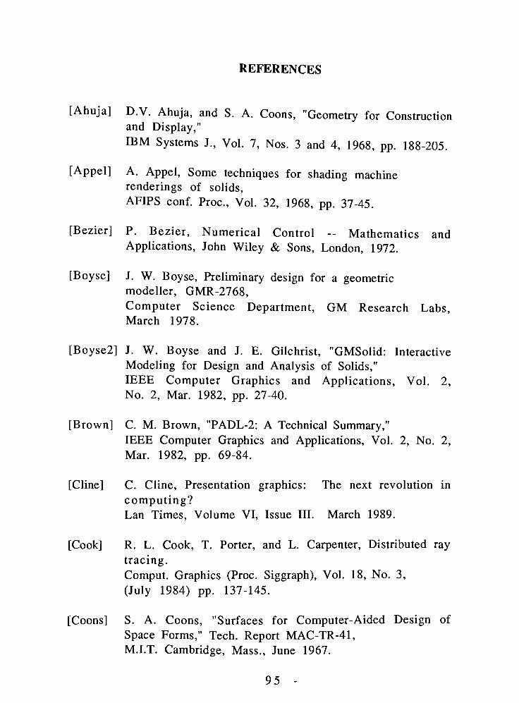
REFERENCES

[Ahuja] D.V. Ahuja, and S. A. Coons, "Geometry for Constructionand

Display,"

IBM Systems J., Vol. 7, Nos. 3 and 4, 1968, pp. 188-205.

[Appel] A. Appel, Some techniques for shading machine

renderings of solids,

AFIPS conf. Proc, Vol. 32, 1968, pp. 37-45.

[Bezier] P. Bezier, Numerical Control - Mathematics and

Applications, John Wiley & Sons, London, 1972.

[Boyse] J. W. Boyse, Preliminary design for a geometric

modeller, GMR-2768,Computer Science Department, GM Research Labs,March 1978.

[Boyse2] J. W. Boyse and J. E. Gilchrist, "GMSolid: Interactive

Modeling for Design and Analysis ofSolids,"

IEEE Computer Graphics and Applications, Vol. 2,

No. 2, Mar. 1982, pp. 27-40.

[Brown] C. M. Brown, "PADL-2: A TechnicalSummary,"

IEEE Computer Graphics and Applications, Vol. 2, No. 2,

Mar. 1982, pp. 69-84.

[Cline] C. Cline, Presentation graphics: The next revolution in

computing?

Lan Times, Volume VI, Issue III. March 1989.

[Cook] R. L. Cook, T. Porter, and L. Carpenter, Distributed ray

tracing.

Comput. Graphics (Proc. Siggraph), Vol. 18, No. 3,

(July 1984) pp. 137-145.

[Coons] S. A. Coons, "Surfaces for Computer-Aided Design of

SpaceForms,"

Tech. Report MAC-TR-41,

M.I.T. Cambridge, Mass., June 1967.

95 -

[Forrest] A. R. Forrest, "On Coons and Other Methods for the

Representation of CurvedSurfaces,"

Computer Graphics & Image Processing,Vol. 1, No. 4, Dec. 1972, pp. 341-359.

[Glassnerl]

Andrew S. Glassner, Space subdivision for fast ray

tracing. IEEE CG&A pp. 15-22, October 1984.

[Glassner2]

Andrew S. Glassner, Spacetime ray tracing for

animation. IEEE CG&A, pp. 60-70, March 1988.

[Goldstein]

R. Goldstein and L. Malin, "3D Modelling with the

SynthavisionSystem,"

Proc. First Ann. Conf. Computer

Graphics in CAD/CAM Systems,

April 9-11, 1979, Cambridge, Mass., pp. 244-247.

[Gordon] W. J. Gordon and R. F. Riesenfeld, "B-Spline Curves and

Surfaces,"

in Computer Aided Geometric Design,

R. Barnhill and R. Riesenfeld, eds.,

Academic Press, New York, 1974, pp. 95-126.

[Gujar] U. G. Gujar, V. C. Bhavsar, and N. N. Datar, Interpolation

techniques for 3-D object generation. Comput. &

Graphics, Vol. 12 Nos. 3/4 pp. 541-555, 1988.

[Hakala] D. G. Hakala., R.C. Hillyard, P.J. Malraison, and B.E.

Nourse, "Natural Quadrics in MechanicalDesign,"

Proc. Autofact West, Vol. 1,

CAD/CAM VIII, Nov. 1980, Anaheim, Calif., pp. 363-378.

[Hanrahan]

P. Hanrahan, Ray tracing algebraic surfaces.

Comput. Graphics (Proc. Siggraph), Vol. 17, No. 3, 1983,

pp. 83-89.

96

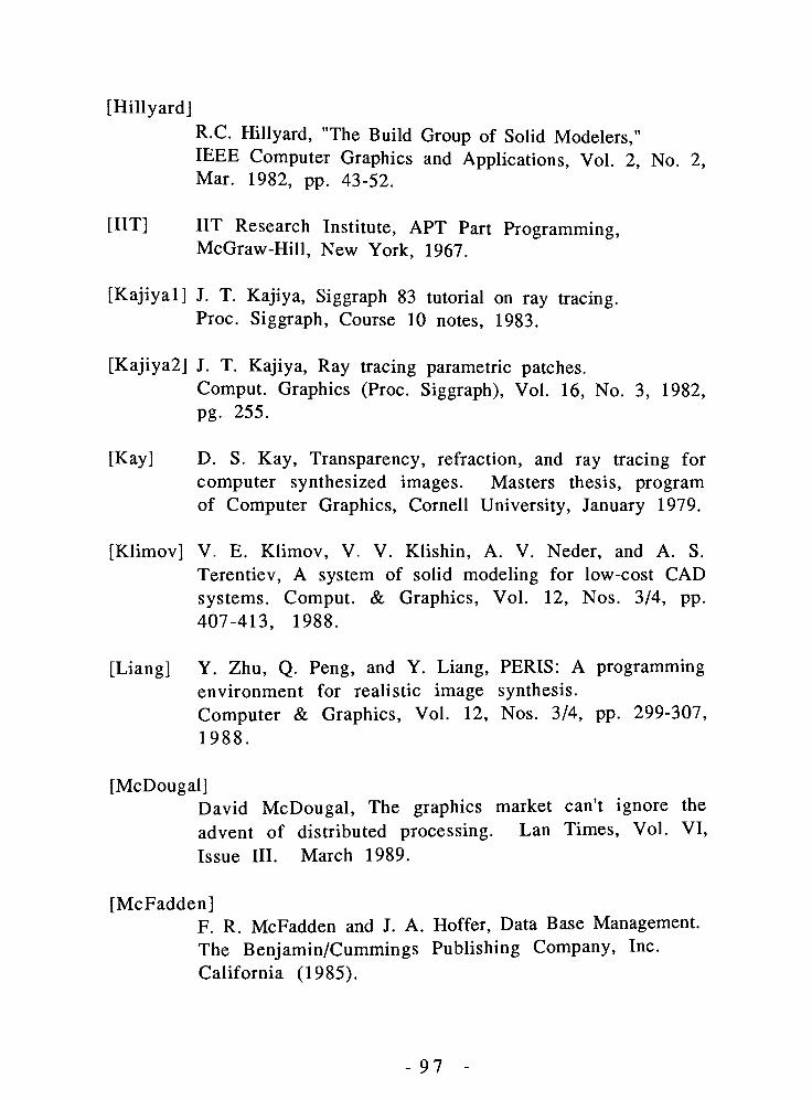
[Hillyard]

R.C. Hillyard, "The Build Group of SolidModelers,"

IEEE Computer Graphics and Applications, Vol. 2, No. 2,Mar. 1982, pp. 43-52.

[IIT] IIT Research Institute, APT Part Programming,

McGraw-Hill, New York, 1967.

[Kajiyal] J. T. Kajiya, Siggraph 83 tutorial on ray tracing.

Proc. Siggraph, Course 10 notes, 1983.

[Kajiya2] J. T. Kajiya, Ray tracing parametric patches.

Comput. Graphics (Proc. Siggraph), Vol. 16, No. 3, 1982,

pg. 255.

[Kay] D. S. Kay, Transparency, refraction, and ray tracing for

computer synthesized images. Masters thesis, program

of Computer Graphics, Cornell University, January 1979.

[Klimov] V. E. Klimov, V. V. Klishin, A. V. Neder, and A. S.

Terentiev, A system of solid modeling for low-cost CAD

systems. Comput. & Graphics, Vol. 12, Nos. 3/4, pp.

407-413, 1988.

[Liang] Y. Zhu, Q. Peng, and Y. Liang, PERIS: A programming

environment for realistic image synthesis.

Computer & Graphics, Vol. 12, Nos. 3/4, pp. 299-307,

1988.

[McDougal]

David McDougal, The graphics market can't ignore the

advent of distributed processing. Lan Times, Vol. VI,

Issue III. March 1989.

[McFadden]

F. R. McFadden and J. A. Hoffer, Data Base Management.

The Benjamin/Cummings Publishing Company, Inc.

California (1985).

97

[Meier] Andreas Meier, Applying relational database techniques

to solid modelling. Computer-Aided Design, Vol. 18,No. 6, July/August 1986, pp. 319-326.

[Mortenson]

M. E. Mortenson, Geometric modeling,

John Wiley & Sons, New York (1985).

[Nagel] R. A. Goldstein, and R. Nagel, 3-D visual simulation.

Simulation, Vol. 16, No. 1, pp. 25-31, January 1971.

[Newman]

W. M. Newman, and R. F. Sproul, Principles of

interactive computer graphics, 2nd ed.,

McGraw-Hill, New York, 1979.

[Okinol] N. Okino, Y. Kakazu, and H. Kubo, "TIPS-I: Technical

Information Processing System for Computer-Aided

Design, Drawing andManufacturing,"

in Computer

Languages for Numerical Control, J. Hatvany, ed.,

North-Holland Pub., Co., Amsterdam, 1973, pp. 141-150.

[Okino2] N. Okino, et al.,"TIPS-I,"

Institute of Presicion

Engineering, Hokkaido University, Sapporo, Japan, 1978.

[Requicha]

A. A. G. Requicha, Representations for rigid solid: theory,

methods, and systems.

ACM Comp. Surveys 12(4), 437-464, (Dec. 1980).

[Roberts] L. G. Roberts, "Machine Perception of Three Dimensional

Solids,"

Tech. Report 315, M.I.T. Lincoln Laboratory,

Lexington, Mass., 1963.

[Rodil] J. Flaquer, and J. L. Rodil, Boolean operations based on

the planar polyhedral representation.

Computer & Graphics, Vol. 12, No. 1, pp. 59-64, 1988.

- 98

[Rogers] David F. Rogers, Procedural elements for computer

graphics. McGraw-Hill Book Company (1985),ISBN 0-07-053534-5.

[Roth] S. D. Roth, Ray Casting for Modeling Solids. Computer

Graphics and Image Processing 18, 109-144 (1982).

[Siska] J. Carlos Siska, 3D solid modeling software development

for industrial and academic purposes. Comput. &

Graphics. Vol. 12, Nos. 3/4, pp. 381-389, 1988.

[Sun] X. Li, Z. Tang, and J. Sun, The implementation of set

operation for regularized geometric object. Comput. &

Graphics Vol. 12, Nos. 3/4, pp. 309-318, 1988.

[Sutty] George J. Sutty, and Steve Blair, Programmer's guide to

the EGA/VGA. Brady Books, a division of Simon &

Schuster, Inc. 1988. ISBN 0-13-729039-X.

[Tang] D. Ma and R. Tang, Realizing the Boolean operations in

solid modeling technique via directed loops.

Comput. & Graphics Vol.12, Nos. 3/4, pp. 319-322, 1988.

[Tech.] "Homogeneous Matrix Representation and

Manipulations of N-DimensionalConstructs,"

Tech. Report 1405, M.I.T. Lincoln Laboratory, Lexington,

Mass., May 1965.

[Tilove] R. B. Tilove, Set membership classification: A unified

approach to geometric intersection problems.

IEEE Trans. Comp. C-29 (10) (Oct. 1980).

[Tokieda]

F. Yamaguchi and T. Tokieda, A unified algorithm for

Boolean shape operations. IEEE Comp.

Graphics Appl. 4 (6) (June 1984).

[Ullner] M. K. Ullner, Parallel machines for computer graphics.

PhD thesis, California Institute of Technology,

Pasedena, Calif., 1983.

- 99 -

[VanDam]

J. D. Foley and A. VanDam, Fundamentals of interactive

computer graphics.

Addison-Wesley Publishing Company (1982),ISBN 0-201-14468-9.

[Veenman]

P. Veenman, "ROMULUS - The Design of a GeometricModeller,"

in Geometric Modelling Seminar,W. A. Carter, ed., P-80-GM-01, CAM-I, Inc.,

Bournemouth, UK, Nov. 1979, pp. 127-152.

[Voelcker]

A. A. G. Requicha and H. B. Voelcker, Solid modeling: a

historical summary and contemporary assessment.

IEEE CG&A (March 1982).

[Whitted]

T. Whitted, An improved illumination model for shaded

display, Comm.

ACM, Vol. 23, No. 6, June 1980, pp. 343-349.

100