rays, waves, and scattering: topics in classical mathematical physics - chapter 1...

chapter1 February 28, 2017

Chapter One

Introduction

Probably no mathematical structure is richer, in terms of the variety ofphysical situations to which it can be applied, than the equations andtechniques that constitute wave theory. Eigenvalues and eigenfunctions,Hilbert spaces and abstract quantum mechanics, numerical Fourieranalysis, the wave equations of Helmholtz (optics, sound, radio),Schrödinger (electrons in matter) ... variational methods, scatteringtheory, asymptotic evaluation of integrals (ship waves, tidal waves,radio waves around the earth, diffraction of light)—examples such asthese jostle together to prove the proposition.

M. V. Berry [1]

There is a theory which states that if ever anyone discovers exactly whatthe Universe is for and why it is here, it will instantly disappear and bereplaced by something even more bizarre and inexplicable. There isanother theory which states that this has already happened.

Douglas Adams [155]

Douglas Adams’s famous Hitchhiker trilogy consists of five books; coincidentallythis book addresses the three topics of rays, waves, and scattering in five parts: (i)Rays, (ii) Waves, (iii) Classical Scattering, (iv) Semiclassical Scattering, and (v)Special Topics in Scattering Theory (followed by six appendices, some of whichdeal with more specialized topics). I have tried to present a coherent account ofeach of these topics by separating them insofar as it is possible, but in a very realsense they are inseparable. We are in effect viewing each phenomenon (e.g. a rain-bow) from several different structural directions or different mathematical levels ofdescription. It is tempting to regard descriptions and explanations as synonymous,but of course they are not. In fact, regarding the rainbow in particular

Aristotle and later scientists in antiquity “constructed theories that primarily describenatural phenomena in mathematical or geometric terms, with little or no concern forphysical mechanisms that might explain them.” This contrast goes to the heart of thedifference between “Aristotelian” and mathematical modeling. [169]

The first two chapters of Part I (Rays) introduce the topic from a physical and amathematical point of view, respectively. Thereafter the subject of rays is viewed inan atmosphere–sea–earth sequence, merging with Part II (Waves) via thereverse sequence earth–sea–atmosphere. Part III (Classical Scattering) examines

© Copyright, Princeton University Press. No part of this book may be distributed, posted, or reproduced in any form by digital or mechanical means without prior written permission of the publisher.

For general queries, contact [email protected]


2 • CHAPTER 1

the relationship between the elegance of the classical Lagrangian and Hamiltonianformulations of mechanics and optics, and having set the scene, so to speak, moveson to develop Kepler’s laws of planetary motion (arising from what I refer to asgravitational scattering). This is followed by a revisitation of the topics of surfacegravity waves, acoustics, electromagnetic scattering (including the Mie solution),and diffraction. Part IV (Semiclassical Scattering) provides a transition from PartIII and addresses more of the nuts and bolts of the underlying mathematics. In sodoing it allows us to reexamine the WKB(J) approximation and apply it to somesimple one-dimensional potentials. Readers may wonder at my notation for thisapproximation—why WKB(J)? It is to pay homage to the legacy of Sir HaroldJeffreys in this and many other areas of applied mathematics and mathematicalphysics. As an eighteen-year-old student I bought a copy of the celebrated Meth-ods of Mathematical Physics [98], co-written with his wife, Lady Bertha Jeffreys.I vowed that I would try to understand as much of it as possible (and I have tried).It is a magnificent book. But writing WKBJ might be a bridge too far, as theysay—the majority of citations in the literature appear to use the WKB form, so Ihave adapted the acronym accordingly. And it appears that I am not the only one tothink Jeffreys deserves more credit than he has been given: see the first quotationin Chapter 22.

Writing the final chapter in this part was a fascinating undertaking; it is a collec-tion of salient properties of Sturm-Liouville systems with particular reference to thetime-independent Schrödinger equation. It touches on several aspects of the theoryof differential equations that have profound implications for the topics in this bookand is distilled from a variety of sources (some of which are now quite difficult tofind). I hope that the reader will benefit from having these all in one place. Part V(Special Topics in Scattering Theory) is an eclectic anthology of material that hasintrigued me over the years, and some of the topics are reflections of joint researchwith recent graduate students. Six appendices round out the material, the second ofwhich is a condensed version of a chapter in [68] (see also [236]). Appendix D isalso based on my contribution to a joint article written with former students [149].

I should also say something about the quotations I have chosen. At the beginningof most chapters I have placed a quotation (and occasionally more than one) froma book, scientific paper, or internet article that I consider to be a brief but pertinentintroduction to the subject matter of that chapter—an appetite-whetter if you will.I have even cited material from Wikipedia (gasp!). In some of the chapters I havemerely waffled on for a bit instead of using an introductory quotation. Regardingshort excerpts from scientific articles on the internet, in the few cases for which Ihave been unable to find the name of the author (after extensive searching), I trustthat the link provided will suffice for the interested reader to pursue the topic (andauthor) further.

In the Preface I mentioned that this book is an intensely personal one, and howthe beautiful phenomenon of a rainbow serves as an implicit template or directoryfor much of the rest of the book. It does so because much of the motivation forthe design of the book springs from it, as evidenced below. And as to why I havechosen to structure things in this way, you will need to read the first paragraph ofthe last chapter (“Back where we started”) to find out!




INTRODUCTION • 3

1.1 THE RAINBOW DIRECTORY

Optical phenomena visible to everyone have been central to the development of,and abundantly illustrate, important concepts in science and mathematics. The phe-nomena considered from this viewpoint are rainbows, sparkling reflections on water,mirages, green flashes, earthlight on the moon, glories, daylight, crystals and thesquint moon. And the concepts involved include refraction, caustics (focal singulari-ties of ray optics), wave interference, numerical experiments, mathematicalasymptotics, dispersion, complex angular momentum (Regge poles), polarisation sin-gularities, Hamilton’s conical intersections of eigenvalues (‘Dirac points’), geometricphases and visual illusions. [151]

The theory of the rainbow has been formulated at many levels of sophistication. Inthe geometrical-optics theory of Descartes, a rainbow occurs when the angle of thelight rays emerging from a water droplet after a number of internal reflections reachesan extremum. In Airy’s wave-optics theory, the distortion of the wave front of theincident light produced by the internal reflections describes the production of thesupernumerary bows and predicts a shift of a few tenths of a degree in the angularposition of the rainbow from its geometrical-optics location. In Mie theory, the rain-bow appears as a strong enhancement in the electric field scattered by the waterdroplet. Although the Mie electric field is the exact solution to the light-scatteringproblem, it takes the form of an infinite series of partial-wave contributions that isslowly convergent and whose terms have a mathematically complicated form. In thecomplex angular momentum theory, the sum over partial waves is replaced by anintegral, and the rainbow appears as a confluence of saddle-point contributions inthe portion of the integral that describes light rays that have undergone m internalreflections within the water droplet. [168]

1.1.1 The Multifaceted Rainbow

What follows is a partial list of context-useful descriptions of a rainbow; they arecertainly not mutually exclusive categories. References are made to (italicized)topics that will be expanded in later chapters, so the reader should not be undulyconcerned about words or phrases in this Chapter that have yet to be defined (e.g., asin the above quotations). Such topics will be unfolded in due course, so be patient,dear reader. But for those who wish to know now whether “the Butler did it,” andif not, who did, the answers are in the back of the book, and it is recommendedthat you turn immediately to the short last chapter, titled “Back Where We Started”prior to returning here.

In part, a rainbow is:(1) A concentration of light rays corresponding to an extremum of the scattering

angleD(i) as a function of the angle of incidence i. In particular it is a minimum forthe primary bow, and the exiting ray at this minimum value is called the Descartesor rainbow ray; as noted below, the notation D(i) is replaced by θ (b) in most ofthe scattering literature, where b is the impact parameter. The angle θ is muchused in connection with the equations of scattering in the chapters that follow, but




4 • CHAPTER 1

(a)

(c)

(b)

(d)

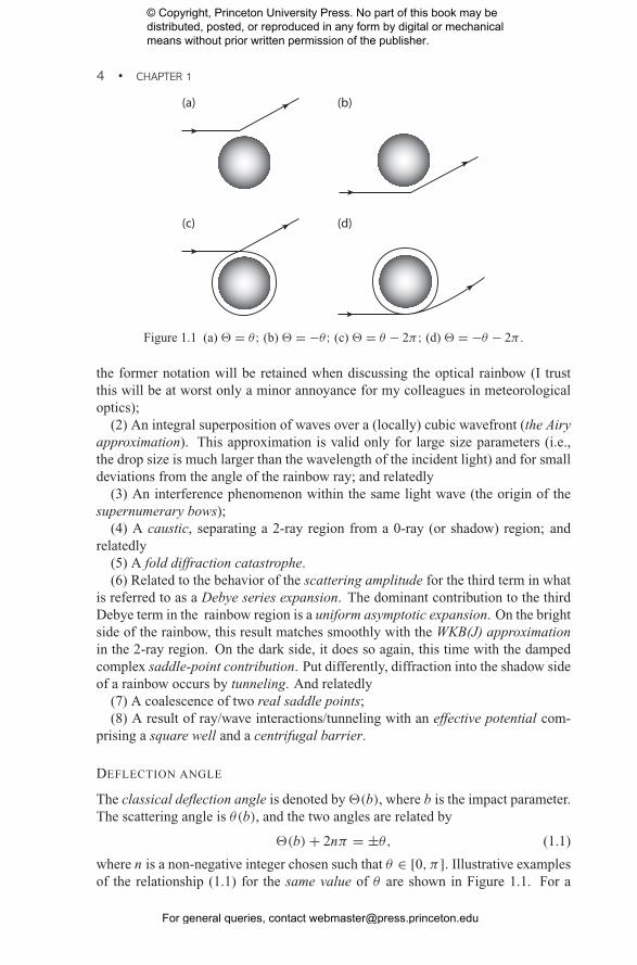
Figure 1.1 (a) � = θ; (b) � = −θ; (c) � = θ − 2π; (d) � = −θ − 2π .

the former notation will be retained when discussing the optical rainbow (I trustthis will be at worst only a minor annoyance for my colleagues in meteorologicaloptics);

(2) An integral superposition of waves over a (locally) cubic wavefront (the Airyapproximation). This approximation is valid only for large size parameters (i.e.,the drop size is much larger than the wavelength of the incident light) and for smalldeviations from the angle of the rainbow ray; and relatedly

(3) An interference phenomenon within the same light wave (the origin of thesupernumerary bows);

(4) A caustic, separating a 2-ray region from a 0-ray (or shadow) region; andrelatedly

(5) A fold diffraction catastrophe.(6) Related to the behavior of the scattering amplitude for the third term in what

is referred to as a Debye series expansion. The dominant contribution to the thirdDebye term in the rainbow region is a uniform asymptotic expansion. On the brightside of the rainbow, this result matches smoothly with the WKB(J) approximationin the 2-ray region. On the dark side, it does so again, this time with the dampedcomplex saddle-point contribution. Put differently, diffraction into the shadow sideof a rainbow occurs by tunneling. And relatedly

(7) A coalescence of two real saddle points;(8) A result of ray/wave interactions/tunneling with an effective potential com-

prising a square well and a centrifugal barrier.

DEFLECTION ANGLE

The classical deflection angle is denoted by�(b), where b is the impact parameter.The scattering angle is θ(b), and the two angles are related by

�(b)+ 2nπ = ±θ, (1.1)

where n is a non-negative integer chosen such that θ ∈ [0, π ]. Illustrative examplesof the relationship (1.1) for the same value of θ are shown in Figure 1.1. For a




INTRODUCTION • 5

repulsive potential (as in Figure 1.1a), � = θ , but in principle for an attractivepotential � can be arbitrarily negative, because the particle (or ray) may orbit thescattering center many times before emerging from it. Thus there may be severaldifferent trajectories that lead to the same scattering angle θ (this will be discussedfurther in Chapter 16).

1.2 A MATHEMATICAL TASTE OF THINGS TO COME

1.2.1 Rays

The Ray-Theoretic Rainbow

A rainbow occurs when the the scattering angle D(i), as a function of theangle of incidence i, passes through an extremum. The folding back of thecorresponding scattered or deviated ray takes place at this extremal scatter-ing angle (the rainbow angle Dmin = θR; note that sometimes in the popu-lar literature the rainbow angle is loosely interpreted as the supplement ofthe deviation, π −Dmin). Two rays scattered in the same direction with dif-ferent angles of incidence on the illuminated side of the rainbow (D > θR)fuse together at the rainbow angle and disappear as the “dark side” (D < θR)is approached. This is one of the simplest physical examples of a foldcatastrophe in the sense of Thom, as will be discussed later. It will also beshown later that rainbows of different orders can be associated with so-calledDebye terms of different orders; the primary and secondary bows correspondto p = 2 and p = 3, respectively, where p > 1 is the number of ray pathsinside the drop, so the number of internal reflections is k = p − 1.

Details

For p − 1 such internal reflections the total deviation is

Dp−1(i) = (p − 1)π + 2(i − pr), (1.2)

where by Snell’s law, r = r(i). This approach can be thought of as the elementaryclassical description.

For the primary rainbow (p = 2),

D1(i) = π − 4r(i)+ 2i, (1.3)

and for the secondary rainbow (p = 3),

D2 = 2i − 6r(i) (1.4)

(modulo 2π ). For p = 2 the angle through which a ray is deviated is

D1(i) = π + 2i − 4 arcsin(

sin i

n

), (1.5)




6 • CHAPTER 1

where n is now the relative refractive index of the medium. In general

Dp−1(i) = (p − 1)π + 2i − 2p arcsin(

sin i

n

), (1.6)

or equivalently,

Dk(i) = kπ + 2i − 2(k + 1) arcsin(

sin i

n

). (1.7)

For p = 2 the minimum angle of deviation occurs when

i = ic = arccos(n2 − 1

3

)1/2

, (1.8)

and more generally when

i = ic = arccos(n2 − 1

p2 − 1

)1/2

, (1.9)

(this clearly places constraints on both n and p if bows are to occur). For theprimary rainbow ic ≈ 59◦, using an approximate value for water of n = 4/3; fromthis it follows that D1(ic) = Dmin = θR ≈ 138◦. For the secondary bow ic ≈ 72◦;andD2(ic) = θR ≈ 129◦. For p = 2, in terms of n alone,D1(ic) = θR (the rainbowangle) is defined by

D1(ic) = θR = 2 arccos

[1

n2

(4− n2

3

)3/2]. (1.10)

1.2.2 Waves

Surprising as it may seem to anyone who thinks in terms of rays alone, there isalso a wave-theoretic approach to the rainbow problem. The essential math-ematical problem for scalar waves can be thought of either in classical terms(e.g., the scattering of sound waves) or in wave-mechanical terms (e.g., thenonrelativistic scattering of particles by a square potential well (or barrier) ofradius a and depth (or height) V0). In either case we can consider a scalarplane wave in spherical geometry impinging in the direction θ = 0 on a pen-etrable (“transparent”) sphere of radius a. The wave function ψ(r) satisfiesthe scalar Helmholtz equation

∇2ψ + n2k2ψ = 0, r < a; (1.11)

∇2ψ + k2ψ = 0, r ≥ a, (1.12)

where n > 1 is the refractive index of the sphere (a similar problem can beposed for gas bubbles in a liquid, for which n < 1). The boundary conditionsare that ψ(r) and ψ ′(r) are continuous at the surface.




INTRODUCTION • 7

1.2.3 Scattering (Classical)

In what follows θ is the angle of observation, measured from the forward to thescattered direction, and thus defines the scattering plane. At large distances fromthe sphere (r � a) the wave field ψ can be decomposed into an incident wave +scattered field:

ψ ∼ eikr cos θ + f (k, θ)r

eikr , (1.13)

where the scattering amplitude f (k, θ) (which can be made dimensionless withrespect to the radius a) is defined as

f (k, θ) = 1

2ik

∞∑l=0

(2l + 1)(Sl(k)− 1)Pl(cos θ). (1.14)

This is the Faxen-Holtzmark formula, and it will be encountered in several differentguises later in the book (e.g., Section 21.5). Sl(k) is an element of the scatteringmatrix (or function or operator, depending on context)) for a given l, and Pl is aLegendre polynomial of degree l. But what is the S-matrix? In optical terms, itis the partial-wave scattering amplitude with diffraction omitted—of course, thisjust kicks the can down the road—what is the partial-wave scattering amplitude?What (really) is diffraction? The reader’s forbearance is requested; for now floatin a sea of relatively undefined terms and just soak. Fundamentally, the S-matrixis the portion of the partial-wave scattering amplitudes that corresponds to a directinteraction between the incoming wave and the scattering particle. In very simplis-tic terms it converts an ingoing wave to an outgoing one, and for a spherical squarewell or barrier we shall find that

Sl = −h(2)l (β)

h(1)l (β)

{ln′ h(2)l (β)− n ln′ jl(α)ln′ h(1)l (β)− n ln′ jl(α)

}, (1.15)

where, following the notation of [26], ln′ represents the logarithmic derivativeoperator, and jl and hl are spherical Bessel and Hankel functions, respectively.β = 2πa/λ ≡ ka is the dimensionless external wavenumber, and α = nβ is thecorresponding internal wavenumber. Sl may be equivalently expressed in terms ofcylindrical Bessel and Hankel functions. The lth partial wave in the Mie solution isassociated with an impact parameter

bl =(l + 1

2

)k−1, (1.16)

that is, only rays hitting the sphere (bl � a) are significantly scattered, and thenumber of terms that must be retained in the Mie series to get an accurate resultis of order β. As implied earlier, for visible light scattered by water droplets in




8 • CHAPTER 1

the atmosphere, β ∼ several thousand. This is why, to quote Arnold Sommerfeld[170]:

The electromagnetic study of light diffraction on an object is a very complicatedproblem even in the case of the sphere, the simplest possible one. The fieldoutside a sphere can be represented by series of spherical harmonics and Besselfunctions of half-integer indices. These series have been discussed by G. Miefor colloidal particles of arbitrary compositions. But even there a mathematicaldifficulty develops which quite generally is a drawback of this method of seriesdevelopment: for fairly large particles (β = ka, a = radius, k = 2π/λ) theseries converge so slowly that they become practically useless. Except for thisdifficulty, we could, in this way, obtain a complete solution of the problem ofthe rainbow.

This problem can be remedied by using the Poisson summation formula (relatedto the Watson transform) to rewrite f (k, θ) in terms of the integral

f (β, θ) = i

β

∞∑m=−∞

(−1)m∞∫0

[1− S(λ, β)]Pλ− 12(cos θ)e2imπλλdλ. (1.17)

For fixed β, S(λ, β) is a meromorphic function of the complex variable λ = l +1/2, which should not be confused with the wavelength (the context should alwaysmake this distinction clear). In particular in what follows it is the poles of thisfunction that are of interest. In terms of cylindrical Bessel and Hankel functions,they are defined by the condition

ln′H(1)λ (β) = n ln′ Jλ(α), (1.18)

and are called Regge poles in the scattering theory literature (see, e.g., [51]).Typically they are associated with surface waves for the impenetrable sphere prob-lem; for the transparent sphere two types of Regge poles arise—one type leadingto rapidly convergent residue series (diffracted or creeping rays), and the other typeassociated with resonances via the internal structure of the potential. Many of theseare clustered close to the real axis, spoiling the rapid convergence of the residueseries. Mathematically, the resonances are complex eigenfrequencies associatedwith the poles λj of the scattering function S(λ, k) in the first quadrant of the com-plex λ-plane; they are known as Regge poles (for real β). The imaginary parts ofthe poles are directly related to resonance widths (and therefore lifetimes). As theindex j decreases, Re λj increases and Im λj decreases very rapidly (reflecting theexponential behavior of the barrier transmissivity). As β increases, the poles λjtrace out Regge trajectories, and Im λj tends exponentially to zero. When Re λjpasses close to a “physical” value, λ = l + 1/2, it is associated with a resonance inthe lth partial wave; the larger the value of β, the sharper the resonance becomesfor a given node number j .




INTRODUCTION • 9

In [83] it is shown that

S(λ, β) = H(2)λ (β)

H(1)λ (β)

⎛⎝R22(λ, β)+ T21(λ, β)T12(λ, β)

H(1)λ (α)

H(2)λ (α)

∞∑p=1

[ρ(λ, β)]p−1

⎞⎠ ,

(1.19)where

ρ(λ, β) = R11(λ, β)H(1)λ (α)

H(2)λ (α)

. (1.20)

This is the Debye expansion, arrived at by expanding the expression[1− ρ(λ, β)]−1 as an infinite geometric series. R22, R11, T21, and T12 are, respec-tively, the external/internal reflection and internal/external transmission coefficientsfor the problem. This procedure transforms the interaction of wave + sphere intoa series of surface interactions. In so doing it unfolds the stationary points of theintegrand, so that a given integral in the Poisson summation contains at most onestationary point. This permits a ready identification of the many terms in accor-dance with ray theory. The first term inside the parentheses represents direct reflec-tion from the surface. The pth term represents transmission into the sphere (via theterm T21) subsequently bouncing back and forth between r = a and r = 0 a totalof p times with p − 1 internal reflections at the surface (this time via the R11termin ρ). The middle factor in the second term, T12, corresponds to transmission tothe outside medium. In general, therefore, the pth term of the Debye expansionrepresents the effect of p + 1 surface interactions.

1.2.4 Scattering (Semiclassical)

On the way to the scattering representation, so to speak, there is a semiclassicaldescription. In a primitive sense, the semiclassical approach is the ‘geometric mean’between classical and quantum mechanical descriptions of phenomena in whichinterference and diffraction effects enter the picture. The latter do so via the tran-sition from geometrical optics to wave optics. This is a characteristic feature of the‘primitive’ semiclassical formulation. Indeed, the infinite intensities predicted by geo-metrical optics at focal points, lines and caustics in general are “breeding grounds”for diffraction effects, as are light/shadow boundaries for which geometrical opticspredicts finite discontinuities in intensity. Such effects are most significant when thewavelength is comparable with (or larger than) the typical length scale for variation ofthe physical property of interest (e.g. size of the scattering object). Thus a scatteringobject with a “sharp” boundary (relative to one wavelength) can give rise to diffractivescattering phenomena.

There are ‘critical’ angular regions where the primitive semiclassical approximationbreaks down, and diffraction effects cannot be ignored, although the angular rangesin which such critical effects become significant get narrower as the wavelengthdecreases. Early work in this field contained transitional asymptotic approximationsto the scattering amplitude in these ‘critical’ angular domains, but they have verynarrow domains of validity, and do not match smoothly with neighboring




10 • CHAPTER 1

‘non-critical’ angular domains. It is therefore of considerable importance to seekuniform asymptotic approximations that by definition do not suffer from thesefailings. Fortunately, the problem of plane wave scattering by a homogeneous sphereexhibits all of the critical scattering effects (and it can be solved exactly, in principle),and is therefore an ideal laboratory in which to test both the efficacy and accuracy ofthe various approximations. Furthermore, it has relevance to both quantum mechan-ics (as a square well or barrier problem) and optics (Mie scattering); indeed, it alsoserves as a model for the scattering of acoustic and elastic waves, and was studied inthe early twentieth century as a model for the diffraction of radio waves around thesurface of the earth. [88]

It transpires that the integral for f (β, θ) can be expressed as an infinite sum:

f (β, θ) = f0(β, θ)+∞∑p=1

fp(β, θ), (1.21)

where

f0(β, θ) = i

β

∞∑m=−∞

(−1)m∫ ∞

0

[1− H

(2)λ (β)

H(1)λ (β)

R22

]Pλ− 1

2(cos θ) exp(2imπλ)λdλ.

(1.22)

The expression for fp(β, θ) involves a similar type of integral for p ≥ 1. Theapplication of the modified Watson transform to the third term (p = 2) in the Debyeexpansion of the scattering amplitude shows that it is this term which is associatedwith the phenomena of the primary rainbow. More generally, for a Debye term ofgiven order p, a rainbow is characterized in the λ-plane by the occurrence of tworeal saddle points λ̄ and λ̄′ between 0 and β in some domain of scattering angles θ ,corresponding to the two scattered rays on the light side. As θ → θ+R the two saddlepoints move toward each other along the real axis, merging together at θ = θR .As θ moves into the dark side (θ < θR), the two saddle points become complex,moving away from the real axis in complex conjugate directions. Therefore, froma mathematical point of view, a rainbow can be defined as a coalescence of twosaddle points in the complex angular momentum plane (see Figure 1.2).

Thus the rainbow light/shadow transition region is associated physically withthe confluence of a pair of geometrical rays and their transformation into complexrays; mathematically this corresponds to a pair of real saddle points merging intoa complex saddle point. Then the problem is to find the asymptotic expansion ofan integral having two saddle points that move toward or away from each other.The generalization of the standard saddle-point technique to include such problemswas made by Chester et al. [164] and using their method, Nussenzveig [84] wasable to find a uniform asymptotic expansion of the scattering amplitude that wasvalid throughout the rainbow region and that matched smoothly onto results forneighboring regions. The lowest order approximation in this expansion turns out tobe the celebrated Airy approximation, which, despite several attempts to improveon it, was the best approximate treatment prior to the analyses of Nussenzveig andcoworkers. However, Airy’s theory had a limited range of applicability as a result




INTRODUCTION • 11

Im λ

0Re λ

Real rays

Rainbow ray

Complex ray

Figure 1.2 The coalescence of two real saddle points in the complex λ-plane as the rainbowangle is approached.

of its underlying assumptions; by contrast, the uniform expansion is valid over amuch larger range.

1.2.5 Caustics and Diffraction Catastrophes

An alternative way of describing the rainbow phenomenon is by way of catastro-phe theory, the rainbow being one of the simplest examples in catastrophe optics.Before summarizing the mathematical details of the basic rainbow diffractioncatastrophe, it will be useful to introduce some of the language used in catastrophe-theoretic arguments. As we know from geometrical optics the primary bow devia-tion angleD1 (in particular) has a minimum corresponding to the rainbow angle (orDescartes ray) Dmin = θR when considered as a function of the angle of incidencei. Clearly the point (i,D1(i)) corresponding to this minimum is a singular point(approximately (59◦, 138◦)) insofar as it separates a two-ray region (D1 > Dmin)from a zero-ray region (D1 < Dmin) in the geometrical-optics level of description.This is a singularity or caustic point. The rays form a directional caustic atthis point, and this is a fold catastrophe (symbol:A2), the simplest example of acatastrophe. It is the only stable singularity with codimension one (thedimensionality of the control space (one) minus the dimensionality of the singular-ity itself, which is zero). In space the caustic surface is asymptotic to a cone withsemi-angle 42◦.

Optics is concerned to a great extent with families of rays filling regions of space;the singularities of such ray families are caustics. For optical purposes this levelof description is important for classifying caustics using the concept of structuralstability: this enables one to classify those caustics whose topology survives pertur-bation. Structural stability means that if a singularity S1 is produced by a generatingfunction φ1 (see below for an explanation of these terms), and φ1 is perturbed to




12 • CHAPTER 1

φ2, the correspondingly changed S2 is related to S1 by a diffeomorphism of thecontrol set C (that is by a smooth reversible set of control parameters; in otherwords a smooth deformation). In the present context this means, in physical terms,that distortions of incoming wavefronts by deviations of the raindrop shapes fromtheir ideal spherical form does not prevent the formation of rainbows, though theremay be some changes in the features. Another way of expressing this concept isto describe the system as well-posed in the limited sense that small changes inthe input generate correspondingly small changes in the output. For the so-calledelementary catastrophes, structural stability is a generic (or typical) property ofcaustics. Each structurally stable caustic has a characteristic diffraction pattern,the wave function of which has an integral representation in terms of the standardpolynomial describing the corresponding catastrophe. From a mathematical pointof view these diffraction catastrophes are especially interesting, because they con-stitute a new hierarchy of functions, distinct from the special functions of analysis.A review of this subject has been made by Berry and Upstill [102] wherein may befound an introduction to the formalism and methods of catastrophe theory as devel-oped particularly by Thom [171] but also by Arnold [173]. The books by Gilmore[105] (Chapter 13 of which concerns caustics and diffraction catastrophes) and Pos-ton and Stewart [172] are noteworthy in that they also provide many applications.

Diffraction can be discussed in terms of the scalar Helmholtz equation in somespatial regionR,

∇2ψ(R)+ k2n2(R)ψ(R) = 0, (1.23)

for the complex scalar wavefunctionψ(R), k being the free-space wavenumber andn the refractive index. The concern in catastrophe optics is to study the asymptoticbehavior of wave fields near caustics in the short-wave limit k→∞ (semiclassicaltheory). In a standard manner, ψ(R) is expressed as

ψ(R) = a(R)eikχ(R), (1.24)

where the modulus a and the phase kχ are both real quantities. To the lowestorder of approximation χ satisfies the Hamilton-Jacobi equation, and ψ can bedetermined asymptotically in terms of a phase-action exponent (surfaces of con-stant action are the wavefronts of geometrical optics). The integral representationfor ψ is

ψ(R) = e−inπ/4(k

2π

)n/2 ∫...

∫b(s;R) exp[ikφ(s;R)]dns, (1.25)

where n is the number of state (or behavior) variables s, and b is a weight function.In general there is a relationship between this representation and the simple rayapproximation [102]. According to the principle of stationary phase, the main con-tributions to the above integral for given R come from the stationary points (i.e.,those points si for which the gradient map ∂φ/∂si vanishes) caustics are singular-ities of this map, where two or more stationary points coalesce. Because k→∞,the integrand is a rapidly oscillating function of s, so other than near the points si ,destructive interference occurs and the corresponding contributions are negligible.The stationary points are well separated, provided R is not near a caustic; the




INTRODUCTION • 13

simplest form of stationary phase can then be applied and yields a series of termsof the form

ψ(R) ≈∑μ

aμ exp[igμ(k,R)], (1.26)

where the details of the gμ need not concern us here. Near a caustic, however, twoor more of the stationary points are close (in some appropriate sense), and theircontributions cannot be separated without a reformulation of the stationary phaseprinciple to accommodate this [164]. The problem is that the “ray” contributionscan no longer be considered separately; when the stationary points approach closerthan a distance O(k−1/2), the contributions are not separated by a region in whichdestructive interference occurs (See Appendix A for the “order” nomenclature usedthis book). When such points coalesce, φ(s;R) is stationary to higher than firstorder, and quadratic terms as well as linear terms in s − sμ vanish. This implies theexistence of a set of displacements dsi , away from the extrema sμ, for which thegradient map ∂φ/∂si still vanishes, that is, for which

∑i

∂2φ

∂si∂sjdsi = 0. (1.27)

The condition for this homogeneous system of equations to have a solution (i.e.,for the set of control parameters X to lie on a caustic) is that the Hessian

H(φ) ≡ det(∂2φ

∂si∂sj

)= 0, (1.28)

at points sμ(X) where ∂φ/∂si = 0 (details can be found in [102] ). The causticdefined by H = 0 determines the bifurcation set for which at least two stationarypoints coalesce (in the present circumstance this is just the rainbow angle). In viewof this discussion there are two other ways of expressing this: (i) rays coalesce oncaustics, and (ii) caustics correspond to singularities of gradient maps. To rem-edy this problem the function φ is replaced by a simpler “normal form” with thesame stationary-point structure; the resulting diffraction integral is evaluatedexactly. This is where the property of structural stability is so important, becauseif the caustic is structurally stable it must be equivalent to one of the catastrophes(in the diffeomorphic sense described above). The result is a generic diffractionintegral that will occur in many different contexts. The basic diffraction catastro-phe integrals (one for each catastrophe) may be reduced to the form

�(X) = 1(2π)n/2

∫...

∫exp[i (s;X)]dns, (1.29)

where s represents the state variables and X the control parameters (for the caseof the rainbow there is only one of each, so n = 1). These integrals stably rep-resent the wave patterns near caustics. The corank of the catastrophe is equal ton: it is the minimum number of state variables necessary for to reproduce thestationary-point structure of φ; the codimension is the dimensionality of the controlspace minus the dimensionality of the singularity itself. It is interesting to note thatin ray catastrophe optics, the state variables s are removed by differentiation (the




14 • CHAPTER 1

vanishing of the gradient map); in wave catastrophe optics they are removed byintegration (via the diffraction functions). For future reference we state the func-tions (s;X) for both the fold (A2) and the cusp (A3) catastrophes; the list for theremaining five elementary catastrophes can be found in the references above. Forthe fold

(s;X) = 1

3s3 +Xs, (1.30)

and for the cusp

(s;X) = 1

4s4 + 1

2X2s

2 +X1s.

By substituting the cubic term (1.30) into the integral (1.29), it follows that

�(X) = 1

(2π)1/2

∫ ∞−∞

exp[i

(s3

3+Xs

)]ds = (2π)1/2 Ai(X),

where the integral here denoted by Ai(X) is one form of the Airy integral. It will beencountered in several different guises as we proceed through the book. For X < 0(corresponding to θ > θR) there are two rays (stationary points of the integrand)whose interference causes oscillations in �(X); for X > 0 there is one (com-plex) ray that decays to zero monotomically (and faster than exponentially). Thisdescribes diffraction near a fold caustic. In 1838 the Astronomer Royal Sir GeorgeBiddle Airy introduced this function to study diffraction along the asymptote of acaustic (although he did not express it in these terms) and provided a fundamentaldescription of the supernumerary bows [23]. (There is also a sequel to this paper,published ten years later [268], which contains a transcript of a fascinating let-ter from the British mathematician Augustus De Morgan (1806–1871)). As notedabove, this integral (in one form or another) will be a recurring topic in several laterchapters. The corresponding integral for the cusp catastrophe is frequently referredto as the Pearcey integral [157].



rays, waves, and scattering: topics in classical mathematical physics - chapter 1...

Documents