re' ad-a286 896 page form approvedno. · 4.7.4 summary of results and assessment of svo(...

Form ApprovedRE' AD-A286 896 PAGE oMB No. 0704-0188

ufdrmaitaionincltheuding nu o mments regardin this burden estmate or any other aspect of this collection ofi2fom4ato. ilding suV 2 1 1 i orate for information Operations and Reports, 1215 Jefferson Dav"s Highway. Suite1204, Arlngto•. VA 2220. Project (0704-0198). Washington, DC 20503.

1. AGENCY USE ONLY (Leave 2. REPORT DATE 3. REPORT TYPE AND DATES COVERED09/00/91 FINAL

4. TITLE AND SUBTITLE 5. FUNDING NUMBERS

COMPREHENSIVE MONITORING PROGRAM, FINAL AIR QUALITY DATA ASSESSMENT REPORT FORFY90. VERSION 3.1 N O NE

NONE

6. AUTHOR(S)

7. PERFORMING ORGANIZATION NAME(S) AND ADDRESS(ES) 8. PERFORMING ORGANIZATION

ROBERT L. STOLLAR AND ASSOCIATES REPORT NUMBER

91311 RO 1

9. SPONSORING/MONITORING AGENCY NAME(S) AND ADDRESS(ES) 10. SPONSERING/MONITORINGAGENCY REPORT NUMBER

11. SUPPLEMENTARY NOTES

NONE

12a. DISTRIBUTION/AVAILABILITY STATEMENT 12b. DISTRIBUTION CODE

APPROVED FOR PUBLIC RELEASE- DISTRIBUTION IS UNLIMITED

13. ABSTRACT (Maximum 200 words)

THE OBJECTIVE OF THIS CMP IS TO: VERIFY AND EVALUATE POTENTIAL AIR QUALITY HEALTH HAZARDS, TO VERIFY PROGRESSTHAT HAS BEEN MADE TO DATE IN REMOVING CONTAMINANTS RESULTING FROM PREVIOUS ACTIVITIES, TO PROVIDE BASELINEDATA FOR THE EVALUATION OF PROGRESS THAT WILL BE MADE IN FUTURE REMEDIAL ACTIVITIES, TO DEVELOP REAL-TIMEGUIDELINES. STANDARD PROCEDURES AND DATA COLLECTION METHODS, AS APPROPRIATE, TO INDICATE IMPACTS OF ONGOING.REMEDIAL ACTIONS, AND TO VALIDATE AND DOCUMENT DATABASE RELIABILITY.

96-01809\3UIUllIUUlt e 6 9 0 9

14. SUBJECT TERMS 15. NUMBER OF PAGES

CONTAMINANT SOURCES. HEALTH AND SAFETY. METEOROLOGY 4 VOLS.

16. PRICE CODE

17. SECURITY CLASSIFICATION 18. SECURITY CLASSIFICATION 19. SECURITY CLASSIFICATION 20. LIMITATION OF ABSTRACTOF REPORT OF THIS PAGE OF ABSTRACT

UNCLASSIFIED I I I _I

NSN 7540-01-280-5500 Standard Form 298 (Rev. 2-89)Prescribed by ANSI Sid. D39.IS

91311R01VERSION 3.1VOLUME III2ND COPY

.1

COMPREHENSIVE MONITORING PROGRAM

Contract Number DAAAi5-87-0095

AIR QUALITY DATA ASSESSMENT .REPORT•.1 :MOR FY90 S

• FINAL REPORT

SEPTEMBER 1991

Version 3.1Volume III

Prepared by*.

R. L. STOLLAR & ASSOCIATES INC.HARDING LAWSON ASSOCIATES2 EBASCO SERVICES INC.

DATACHEM, INC.I :MIDWEST RESEARCH INSTITUTE

S, Prepared for:

U. S. ARMY PROGRAM MANAGER FORROCKY MOUNTAIN ARSENAL

THE VIEWS, OPINIONS, AND/OR FINDINGS CONTAINED IN TillS REPORT ARE THOSE OFTHE AUTHOR(S) AND SHOULD NOT BE CONSTRUED AS AN OFFICIAL DEPARTMENT OF

-. bk• THE ARMY POSITION. POLICY, OR DECISION,. UNLESS SO DESIGNATED 3Y OTHERDOCUMENTATION.THE USE OF TRADE NAMES IN THIS REPORT DOES NOT CONSTITUTE AN OFFICIALENDORSEMENT OR APPROVAL OF THE USE OF SUCH COMMERCIAL PRODUCTS. THE

REPORT MAY NOT BE CITED FOR PURPOSES OF ADVERTISEMENI.

PRINTED ON RECYCLED PAPERVDTIC QUALITY [ 23PECLrED 3

' 0

*

DISCLAIMER NOTICE

THIS DOCUMENT IS BEST

QUALITY AVAILABLE. THE COPY

FURNISHED TO DTIC CONTAINED

A SIGNIFICANT NUMBER OF

COLOR PAGES WHICH DO NOT

REPRODUCE LEGIBLY ON BLACK

AND WHITE MICROFICHE.

ILi i @@ @ @ @@ II

,, • . -:.i.7 _., =::•:'•__':•f .'_••:__ 0- 0- 0•• • m • • -" •• 6 0 S- .. •.. ."

0

TABLE OF CON IINTS

PAGE 0

vOUy

EXECUTIVE SUM MARY ................................................... I

1.0 IN I k2ODUCTION ...................................................... I 0

1. 1 SITE BACKGROUND INFORMATION ....................................... 41.2 POTENTIAL CONTAMINANT SOURCES ..................................... 4

1.2.1 SOUTH PLANTS MANUFACTURING COMPLEX ........................... 81.2.2 BASIN A ................................................... 81.2.3 BASIN F ................................................... 9

1.2.3.1 Background of Previous Studies ............................ 91.2.3.2 Impacts of Basin F Remediation on CMP .................... 10

1.2.4 OTHER POTENTIAL CONTAMINANT SOURCE AREAS ...................... 101.2.5 FINDINGS 'IF TIIE AIR REMEDIAL INVESTIGATION PROGRAM .............. I I1.2.6 RESULTS OF THE CMP FY88 AND FY89 ASSESSMENTS ................. 12

2.0 REGIONAL AND LOCAL AIR QUALITY AND METEOROLOGICALCh IARACTER ISTICS .................................................. 15

2.1 A IR Q UALITY ..................................................... 15

2.1.1 PARTICULATES .................. ! .......................... 152,1.2 M ETALS .................................................. 192.1.3 SULFUR DIOXIDE ........................ .................... 192.1.4 NITROGEN OXIDESS .......................................... 20

2.1.5 OZONE...................... ............*.......... ... ** .......... **,**212.1.6 CARBON M ONOXIDE ......................................... 21

2.2 METEOROLOGY AND AIR QUALITY DISPERSION ............................ 22 0

3.0 PROGRAM STRATEGY AND METHIODOLOGY .............................. 30

3.1 G ENERAL BACKGROUND .. ................. ........................... 303.2 CMP AIt QUALITY MONITORING PROCRAM ............................... .31

3.2.1 SITING C RITERIA . ................................... ........ 32

3.2.1.1 Proximity to Sources or Boundaries ...................... 323.2.1.2 Wind Speed/Direction ................................... 323.2.1.3 Topographical Features and Obstructions .................. 393.2.1.4 "ontinuity With Previous Monitoring Programs ............. 39

3.2.2 'tiE CMI, AIR QUAiITY MONITOItNG NETWORK LOCATIONS ............. 40

3.2.2.1 Permanent Stations Locations ........................... 403.2.2,2 Portable Air Quality Monitoring Stationis ..... ................. 40

3,2.3 AIR QUALITY MONITORING STRH;'rEGIES ........................... 41

3.2.3.1 Baseline Assessment .................................... 41

•- I

tAIR -90.TOCR.v. 08/28/.1.

.- .• .rmrT~r ~-

TABLE Or CONTENTS (continued])

PAGE

3.2.3.2 Worst-case Assessment..................................... 443.?. 3.3 Remedial Assessment............................. 453.2.3.4 Criteria for Gaseous Pollutant Asscssment.............45

.13.2.4 AIR QUALITY MONITORING METHODS................................. 46 0

3.2.4.1 Total Suspended Particulates (TSP).......................... 463.2.4.2 Particulate Matter Less than 10 Microns (PM-10).............. 473.2.4.3 Asbestos............................. ................... 473.2.4A4 Volatile Organic Compounds................................ 47

3245 Semi-volatile Organic Compounds ........................... 483.2.4.6 ICP Metals and Arsenic.................................... 483.2.4,7 Organochlorine Pesticides (0OC?)............................ 493.2.4.8 Mercury..................... ........................... 49

3.3 THlE BASIN F REMEDIATION AIR MONITORING PROGRAM......................... 493.4 THE IRA-F AIR QUALITY MONITORING PROGRLAM............................. 52

'A.4 1 S MPLNG L CAT ONS .... ... ... .... ... ... .... ... . 53.4.2 SAMPLING LOCATIOS............................................... 52

3.4.3 CAP AND VENT MONITORING........................................55S

3.5 METEOROLOGICAL MONITORING PRocKAM......................... ............ 55

3.5.1 LOCATION OF MIETEOROLOGICAL MONITORING STATIONS................. 5503.5.2 MONITORING EQUIPMENT AND STRATEGY.............................. 573.5.3 DA:TA ACQUISITION................................................ 573.5.4 DATA APPLICATIONS............................................... 58

3.6 CONTINUOUS Alit MONITORING PROGRAM..................................... 59"3.7 L.ABORATORY ANALYSIS PROGRAM........................... ............... 59

"O'LUJME 11

4.0 RESULTS OF: FY90 PROGRAM...................... ....................... 64

4.1 BASIS OF AIR QUALITY DATA EVAL.UATION.................................... 64

4.1.1 COMPUTERIZED D)OCUMENTATION......................... ........... 654.1.2 REME'DIATION E-VALUATION ......................................... 674.1.3 D)ISPERSION MODEL APPLICATIIONS.................................. 04.1 .4 SOURCE EMISSION FACTORS..................................... .... /14

4.2 TOTAL SUSPENDEFD PARTICULATES (TSP)................................ ... i 15

4.2.1 CMP F.Y90 TsIP RESULTS............................754.2.2 ASSESSMENT OF BASIN FT'S1~Po R-EM'ED'IAlI,'M'PA'CTS............88

4.2.2.1 CMII SlP Monitoring Results............................... 884.2.2.2 Basin - TsP, Monitoring Results................ ............ 964.2.2.3 Analysis of Combined CMP/Basin 17 TSP Monitoring Rcsults ... 1054.2.2.4 Individual Day Remedial Assossmient Compnrisons............. 110

Alit~~ 1)0'1'(

AIR -!Ji.~LOA

i ' TABLE OIF CONTENTS (continued)

PAGE

4.2.3 RMA TSP CAUSAL EFFECTS ......... ..... ......................... 1104.2.4 DENVER METROPOLITAN AREA TSP INFLUENCES .................... 120

S4.2.4.1 CM P FY90 Period Results ............................. 120

4.2.5 ANALYSIS IMPLICATIONS FOR MITIGATION AND CONTROLS .............. 1254.2.6 SUMM ARY ................................................. 126

4.3 RESPIRABLE PARTICULATI, MATTER .................................... 126

4.3.1 CMP PM-F) MONITORING PROGRAM ............................. 1264.3.2 BASIN F PM -10 IMPACTS ...................................... 129

4.3.2.1 CMP Data . ......................................... 1294.3.2.2 Basin F Data . ....................................... 1404.3.2.3 Combined Basin F and CMP Data Analysis ................ 140

4.3.3 METROPOLITAN DENVER PM-10 DATA ........................... 144 0

4.3.4 SUMMARY OF PM-10 ANALYSIS .................................. 147

4.4 M ETALS ......... .......................................................... 147

4A4.1 METALS MONITORING STRATEGIES .............................. 1474.4.2 CMP FY90 METALS MONITORING RESULTS ........................ 1484.4.3 ASSESSMENT OF BASIN F METALS IMPACTS ...... ..... ............. 152

4.4.3.1 CM P Data . ......................................... 1524.4.3.2 Basin F Data ... ..................................... 1594.4.3.3 Combined CMP and Basin F Data Analyses ................ 173

4.4.4 ANALYSIS OF METALS SOURCE FACTORS .......................... 1804.4.5 ASSESSMENT OF' METALS CONCENTRATIONS RELATIVE TO TOXIC

G UIDELINES. ............................................... . 1884.4.6 SUMM ARYY ................................................. 191

4.5 A SBE1 STOS .. .......... .. ............. ... .......... ......... ... ... 19 14.6 VOLATILE ORGANIC COMPOUNDS (VOCS) ................................. 192

4.6.1 CMP VOC SAMPLIN.,, ANALYSIS AND) REPORTING STRATEGII..S ........... 1924.6.2 CM1i FY90 VOC MONITOUTNC RESULTS .............. ............. 194

4.6.2.1 Dedemlher 19, 1989 ................................... 2004.6.2.2 June 27, 1990 ..... ................................. 2024.6.2.3 July 18, 1990 ..... .................................. 2024.6.2.4 July 27, 1990 ....................................... 2064.6.2.5 August 9, 1990 . ..................................... 2084.6.2.6 Seplember II, 1990 ................................... 210

4.6.3 BASIN F VOC IMPACTS ......................................... 210

4.6.3.1 C M P Data . ........................................ 210 S4.6.3.2 Basin F D ata ........... ............................ 2214.6.3.3 Combined CMIP and Basin I D)ata Analyses.................. 238

S• '::t AIR 9(I.TOC(

---

......... I IsIm

'1*

TABLE -)F CONTENTS (continued)

PAGE

4.6.4 ADDITIONAL VOC MONITORING CONSIDERATIONS ............. 244

4.6.4.1 Seasonal VOC Impacts ................................ 2444.6.4.2 Metropolitan Denver Area VOC Emissions ................. 247

4.6.5 SUMMARY OF RESULTS AND ASSESSMENT OF VOC TOXICITY LEVELS ..... 2564.6.6 VOC NONTARGET ANALYTE RESULTS ............................ 266

4.6,6.1 Laboratory Procedures ................................. 2664.6.6.2 Summary of Nontarget VOCs ............................... 267

4.7 SEMI-VOLATILE ORGANIC COMPOUNDS (SVOCs) ANI) ORGANOCIILORINE PESTICIDES(O C Ps) ............. ............................................. 272

4.7.1 MONITORING, ANALYSIS AND REPORI~rNG STRATEGIES .................. 2724.7.2 CMP FY90 SEMI-VOLATILE ORGANIC COMPOUNDS MONITORING RESULTS . 274

4.7.2.1 A ugust 2, 1990 .1.................................... 277 •4.7.2.2 A ugust 7, 1990 ..................................... 2804.7.2.3 August 29, 1990 ...................... 280

4.7.3 BASIN F SVOC IMPACTS ................................. .... 284

4.7.3.1 C M P D ata ......................................... 2844.7.3.2 Basin F D ata ....................................... 288

4.7.3.3 Combined CMPI and Basin ! Data Analyses ...... .......... 300

4.7.4 SUMMARY OF RESULTS AND ASSESSMENT OF SVO( ''OXICITY LEVELS .... 3054.7.5 SEASONAL CONSIDERATIONS .................................... 3104.7.6 SVOC NONTARGET ANALYTE RESUILTS ........................... 310

0

VOILUME III

5.0 CONTINUOUS AIR MONITORING PROGRAM ................................ 318

5.1 PROGRAM O VERVIEW ............................................... 3185.2 A NALYSIS O VERVIEW . .............................................. 3215.3 C ARBON M ONOXIDE ................................................ 32 I5.4 O ZONE . ........................................................ .. 3325.5 SULFUR D IOXIDE ............................................... .... 34 15.6 NITRIC OXIDE, NITROGEN DIOXIDE AND NITROGEN ()XIDIES .................... 3515.7 REGIONAL EMISSION SOURCES IMPACTINN RMA ........................... 376

5.7.1 DECEMBER 22-7 1, 1989 . .................................... . .3815.7.2 MAY 21, 1990 .0A

6.0 1P1IOTO VISIS 31ILITY STUDY . .............................. ............ 393

6.1 HIGHI W YND DUST EVENTS . ............................................. 3946.2 BROWN CLOUiD EVENTS ............ ........... ............ 398 •

6.3 SUM M ARY . ................................... ..................... 418

7.0 METEOROLOGY MONITORING AND DISPERSION MOIFI.ING P(ROG(RAMS .... 419

All? 90.1'f•G -

w I I I Iip

0

TABLE OF CONTENTS (continued)

7.1 METEOROLOGY PROGRAM OVERVIEW ................................... 419

7.1.1 PfOCGRAM OBJECTIVES ................................. . 4197.1.2 DATA RECOVERY ........................................... 4207.!.3 DATABASES ................................. ............... 420 0

7.2 SUMMARY OF RESULTS ....... ....................................... 421

7.2.1 TEMPERATURE ............................................. 4247.2.2 RELATIVE HUMIDITY ......................................... 4247.2.3 BAROMETRIC PRESSURE ....................................... 4267.2.4 SOLAR RADIATION ........................................... 4267.2.5 PRECIPITATION ............................................. 4267.2.6 W INDS . ......................... .......................... 4287.2.7 ATMOSPHERIC STABILITY ...................................... 428

7.3 SEASONAL AND DIURNAL INFLUENCES ................................... 4357.4 SUMMARY AND CONCLUSIONS ... ..................................... 4417.5 RMA METEOROLOGICAL STAkTION COMPARISONS ........................... 4437.6 ATMOSPHIERIC DISPERSION MODEL ..................................... 448

7.6.1 M ODEL APPLICATIONS ........................................ 4487.6.2 ADDITIONAL MODEL AI'PROACIIES AND ANALYSES ................... 452

7.6.2.1 Source Emissions Characterization ... .................... 452 07.6.2.2 Remedial Activity Production Data ....................... 4527.6.2.3 Local and Regional Emissions Inventory ................... 4537.6.2.4 Empirical/Statistical Adjustments ....................... 453

8.0 QUALITY ASSURANCE PROGRAM ...................................... 454

8.1 OVERVIEW AND GENERAL GUIDANCE ................................... 454 6

8.2 LABORATORY QUALITY CONTROL AND QUALITY ASSURANCE PROGRAM OVERVIEW .. 4558.3 FIELD QUALITY CONTROL PROGRAM ........................... ........ 451

8.3.1 O RGANIZATION ............................................. 4578.3.2 FIELD PROGRAM QUALITY CONTROI ............ .................. 4578.3.3 QUALITY CONTROL FIELD SkmPiE RESUI.TS ........................ 458 0

8.3.3. 1 VOC Quality Control Results................................ 4588.3.3.2 Semi-Volatile Organics and Organics oui PUF Quality Control

R esults .. .............. .... ... ... .. ... ...... ..... 459

8.3.4 DATA PROCESSING .. ........................................ 4630

8.4 ASSESSMENT OF DATA PRECISION AND COLLOCATED DUPLICATE SAMPLING RESULTS 4648.5 QUALITY ASSURANCE FIELD PROCEDURES ................................ 469

8,5.1 SYSTEM A UDITS ............................................ 4708.5.2 PERFORMANCE AUDITS OF FIEIm SAkmPr,14G EQUIPMENT ................. 4708.5.3 CALIBRATION AND CERTIFICATION OF STANDARDS ................... 471

)0 C O N CILU SIO NS ....................................................... 472

-V .

AIR 90.TOGC"v. O3/28/91

0 a 10

I

TABLE OF CeNI-ENTS (colntinued)

PAGE

9.1 TOTAL SUSPENDED PARTICULATES ...................................... 4729.2 RESPIRABLE PARTICULATES (PM- 10) ................................... 4739.3 M ETALS ......................................................... 4739.4 A SBESTOS .............................. ........................ 4739.5 VOLATILE ORGANIC COMPOUNDS ....... ............................... 4739.6 SEMI-VOLATILE JRGANIC COMPOUNDS .................................. 4749.7 OPGANOCHLORINE PESTICIDES . ....................................... 4749.8 CRITERIA POLLUTANTS ....... . ......................................... 4749.9 GENERAL INTERPRETATIONS .................................. 474

10.0 R EFER EN C ES ....................................................... 476 0

VOLUME IV

APPENDIX A Total Suspended Particulates (T1,P) Data (on diskcttc)

APPENDIX B Respirable Particulates of Less Than 10 Microns (PM-10) Data (on diskette)

APPENDIX C Arsenic, Metals and Mercury liata (on diskette)

APPENDIX D Asbestos Data (on diskette)APPENDIX E Volatile Organic Compounds (VOC) Data (on diskette)

APPENDIX F Semi-Volatile Organic Compounds (SVOC) Data (on diskette)

APPENDIX G Organochlorine Pesticides (OCP) Data (on diskette)

APPENDIX Ht Quality Assurance/Quality Control

APPENDIX I Continuous Air Quality Data

APPENDIX J Air Quality Meteorological Data and Joint Frequency Distribution (on diskette)

APPENDIX K ISC and INPUFF2 EPA Model Description

APPENDIX 1, IRA-4 Total Suspended Particulates (TSP) Data (on diskette)

APPENDIX M IRA-F Respirable Particulates of Less Than 10 Microns (PM.-10) (on diskette)

APPENDIX N IRA-F Arsenic, Metals, and Mercury Data (on diskette)A

APPENDIX 0 IRA-F Volatile Organic Compounds (VOC) Data (on diskette)

=• APPENDIX P IRA-F Soiii--Voiatile Organic Compounds (SVOC) lData (on diskette) •

APPENDIX Q IRA-F Organochlorine Pesticides (OCP) Data (on diskette)

- VI

Ait- 90.TOC 0""6ev- 08/28/91

he!

Table 2.1 -1 Colo-ado and National Ambient Air Quality SiandardsATable 2.2-! Summary of Temperature Data in the RMA Vicinity

TFable 2.2-2 Summary of Precipitation and H-umidity Data in the I(MA Vicinity

Table 2.2-3 Summary of Wind and Pressure Data in the RMA Vicinity

TFable 2.2-4 Summary of Mcteoroiogical Data in the RMA Vicinity

Table 32.-1 Sampling Locations

Table 3.2-2 Parameters and St~ategies for RMA Air Monitoring Programn

Table 3.2-3 Sampling Strategics for High Event..Air Quality Monitoring

TFable 3.4-1 Location and Monitoring Parameters at IRA-F Sites

Table 3.5-1 Meteorological Parameters Monitored at RMA During~ FY90

Table 3.6-1 RMA Continuous Gaseous Air Monitor~apg Program Summm y

T-able 3.7 -1 Analytical Methods for Air Quality Monitoring Program

* Table 3.7-2 Analytes and Certified Reporting Limits for Air Qualihy Monitoring P~rogram

*Table 4. 1-1 Basin F Remnediation Phases

Table 4.1--2 Emissions inventory Summary for Regulated Pollutants

Tablk- 4.2-1 Sumnmary of RMA Total Suspended Particulates (TSP) Monitoring for FY90

T able 4.2-2 Total Suspended P'articulates (TSP) Sampling Results for FY90

Table 4.2-3 Total Suspended Particulates (TSP1) Sampling Results for CMP Phases 1-4

~Table 4.2- 4 Total Suspended P~articulates (TSP) Samipling Results for Basin F/IRA-I2

P~hase,- 1-4

Fable 4.2-5 Combined Seasonal TSlP Concentrations-

1 Table 4.2-6 Seasonial TSP Concentrations by Site

Table 4.2-7 Particulate Sources with Emissions of 25 TPY or More

Table 4.2-.8 Denver Metropolitan Area Total Suspended Particulates (TSP)

Table 4.3-1 Summary of' CMI1 FY90 Sampling for Respirable Particulates of Less Thanl 10Microns (P'M-IC)

Table 4.3-2 Concentrations of Respirable Particulatts of Less Thian 10 Microns (PM- 10) forCMIP FY90

All -90.TO CH- 08/28/91

........ ....

A-

LIST Of1 TAi]1.LS (continued)

Table 4.3-3 Concentrations of Respirable Particulates of Less Than 10 Microns (I'M-10) for

Phases 1-4

* Table 4.3-4 Combined Seasonal PM-10 Concentrations

. Table 4.3-5 Seasonal PM-10 Concentrations by Site

Table 4.3-6 Concentrations of Respirable Parti,.ulates of Less Than t0 Microns for Phases3 and 4 at IRA-F Sites

Table 4.3-7 Denver Metropolitan Area Respirable Particulates of Less Than 10 Microns(PM- 0)

"Table 4.4-I Summary of Routine Metals Sampling for FY90

Table 4.4-2 Summary of CMP Metals Concentrations for FY90

Fable 4.4-3 Summary of CMP Metals Concentrations by Phase

Table 4.4-4 Metals Data Summary for 1986-1987 Remedial Investigation Program

rTable 4.4-5 Summary of Basin F/IRA-F/RIFS Metals Concentrations for Phases 1-4

Fable 4.4 -6 Observed Maximum Metals Concentrations and Associated Wind Speed at CMPSites S

Table 4.4-7 Seasonal Metals and Arsenic Concentrations by Site

Table 4.4-8 Maximum Concentrations Measured at RMA for CMP and Basin F/IRA-F:

Concurrent Programs

Table 4.4-9 RMA Target Metals Compounds Comparison to Hlealth Guidelines

Table 4.5-I Synopsis of FY90 Asbestos Monitoring

Table 4.6-1 Synopsis of FY90 Monitoring for Volatile Organic Compounds (VOC)

Table 4.6-2 Summary of FY90 Volatile Organic Compounds (VOC) Concentrations

S Trable 4.6-3 Summary of CMMP Volatile Organic Conpounds (VOC) Concentrations forPhase% 1-4

Table 4.6-4 Summar3 of Basin F/IRA-F/RIFS V1OC Concentrations for Phases 1-4

Table 4.6-5 Maximum Concentrations and Locations of Volatile Organic Compounds

Fable 4.6-6 Combined Seasonal Average VOC Concentrations

Table 4.6-7 Volatile Organic Compounds (VOC) Sources with Emissions of 10 TIY or More

Table 4.6-8 Total Releases of Toxic Chemicals by Facility and Toxicity for Denver andAdams Counties

TFable 4.6-9 Releases of Toxic Chemicals for Denver and Adams Counties

... viii -

AIR -90.TOG 0Rev. 08/28/91

V 00 0•000 6 4

I- -i- -.-

Llis~l ol-. TA[1LE-S (continued)

fa ble 4.6 -10 RMA Target Volatile Organic Ccompounds (VOC) Comparison to HealthGuidelines for Phases I and 2

Table 4.6-I I RN4A Target Volatile Organic Compounds (VOC) Comp'irison to HecalthGuidelines for Phases 3 and 4

'rable 4.6-12 Comparison of EPA Air Toxics Study and RMA Results for VOCs

Tabkt 4.6- 13 Ambient Volatile Organic Compounds (VOC) Conccntrat ions from Various

Table 4.6-14 Summary of VOC Noritargets for FY90

Table 4.6-15 Summary of VOC Blank Nontargets for FY90

Table 4.7-1 Synopsis of FY90 Semni-Volatile Organic Compounds (SVOC) Monitoring

Table 4.7-2 Synopsis of F-Y90 Organochlorine Pesticides (OCP) Monitoring

TFable 4.7- 3 Summary of Semi-Volatile Organic Compounds (SVOC) Concentiations for1-Y90'- Pesticide Method

Table 4.7-4 Summary of Orgatiochlorine Pesticides (O{1Cl) Concentrations for FY90

Table 4-7-5 Summary of CMP Semi-Volatile Organic Compounds (SVOC) Concentrations

Table ~ ~ b Ph- Smasyofe Organochlorine Peticide (OCP) Concetratin by Phlase

*Table 4.7-7 Sunmmary of Basin F-/IRA--F/RIFS Semi-Volatile Organic Compounds (SVOC)for Phases 1-4

T able 4-7--8 Maximum Average Long-Termi and Shiort-Termn Semi- Volatile OrganicCompounds Concentrations

T able 4.7-9 RMA Tar get SVOC and OCP Comparison to Health Guidelines

Table 4.7-10 Combined Seasonal Organochiorine Poesticides (0(1') Concent rat ions

'Fable 4,7 -Il Summinary of SVOC Nonitargets for FY9O

Table 4.7.- 12 Summary of SVOC Nontargets Blank D)ata for FY90

Fabl 5.1-1 RMA arid Coloradc Depar tment off Health Gaseous Eminissions Monitoring S'Itec

'Fable 5.3-1 Summary of Carbon Monoxide I-Hlour Average Values in pp ii October 1, 1989-ý IV (00 IST thro ugh SePtembco' 30, 1990 (2400 IVST)

Table 5.3-2 Summary of Carbon Monoxide 8-H1our Average Values in ppmi October 1, 1989(0 10(0 MS) through Septembe~r 30, 1990 (2400 MSTl)

'rable 5.4-1 Summary of'Ozone I-Hiour Average Values in ppm October I, 1989 (0100 MST)thiough September 30, 1990 (2400 MST)

Alit 90TOU

H". 08/29/0901

LIST OF TAIILES (continued)

Table 5.5-1 Summary of Sulfur Dioxide I-Hour Average Values in ppm October i, 1989Aý 1.' •(0100 MSl) through September 30, 1990 (2400 MST)

Table 5.5-2 -,,tnmary of Sulfur Dioxide 3-1tour Average Values in ppm October 1, 1989(0100 MST) through Septembe. 30, 1990 (2400 MST)

Table 5.5-3 Summary of Sulfur Dioxide 24-11our Average Values in ppm October 1 1989(0100 MST) through September 30, 1990 (2400 MST)

Table 5.6-1 Summary of Niti ic Oxide (NO) I -lcur Average Values in ppm October 1, 1989(0100 MST) through September 30, 1990 (2400 MST)

-able 5.6-2 Summary of Nitrogen Dioxide (NO 2 ) I--Hour Average Values in ppm October1, 1989 (0100 MST) through September 30, 1990 (2400 MST)

Fable 5.6-3 Sum-imary of Nitrogen Oxides (NO ) I -ttour Average Values in ppm October I,1989 (0100 MST) through September 30, 1990 (2400 MST)

Tablec 5.7-1 Carbon Monoxide (CO) Souiccs with Emissions of 100 1TPY of More

Table 5.7-2 Sulfur Dioxide (SO 2 ) Sources with Emksions of 40 TPY or More

Table 5.7-3 Nitrogen Oxides (NOx) Sources with Emissions of 40 TPY or Mo-e

Table 5.7-4 Relevant Air Quality and Meteorological Data for December 22-23, 1989

Table 5.7-5 Relevant Air Quality and Meteorological Data for May 21, 1990

Table 6.1--I Summary of High Dust Events During FY90

"" Table 6.1-2 TSP Monitoring Results for May 15, 1990

Table 6.1-3 May 15, 1990 Dust Event Data

Table 6.2-1 October 25, 1989 Brown Cloud Event Data

Table 6.2-2 January 5,1990 Brown Cloud Event Data

Table 6.2-3 September 14, 1990 Brown Cloud -vent Data

Table 7.1-1 Summary of RMA Meteorological Monitoring for FY90

Table 7.2-1 Summary of Rocky Mountain Arsenal Monthly Meteorological Conditions for: i"•T'•;•FY90 (October 1, 1989 through September 30, 1990)

I-able 7.4-I FY89 - FY90 Comparison

of 7Fable 7.5-I Meteoroloý;ical Tower Comparison of Wind Speed (mpl)/l)irection

Table 7.5-2 Meteorological Tower Comparison of Temperature ('F)

Table 7.5-3 Meteorological Tower Comparison of Precipitation (inches)

Fable 7.5--4 FY90 Frequency (%) of Atmospheric Stability Categories for Each Met Station

-A.

AIR -. MTI'OC

Rev. 08/28/91

0......S 0 0 0 0 I

0

LIST OF TABLES (continued)

0

Table 8.3-1 CMP Target Volatile Organic Compounds (VOC) Blank Values

-able 8.3-2 Summary of Smi-Volatile Organic Compounds Results of Field Spiking

Table 8.3-3 Summary of OCP Results of Field Spiking0

Table 8.4-1 Collocated Sample Comparisons for FY90 at AQ5

Table 8.4-2 Continuous Air Quality Parameters Precision Results

0

0

0

ixi

A]I -90 ToC

R

w •

LIST OF FIGURFS

Figure 1.1-1 Rocky Mountain Arsenal Location Map

Figure 1.1-2 Rocky Mountain Arsenal Reference Map

Figure 1.2-1 CMP Air Quality and Meteorological Monitoring Stations 0

Figure 2.2-1 Stapleton Airport Wind Direction Rose, 1982-1986

Figure 3.2-1 CMP Air Quality Monitoring ý,>itions at Rocky Mountain Arsenal

Figure 3.2-2 National Ambient Air Quality Sampling Schedule for 1990

Figure 3.3-1 Location of Basin F Air Quality Monitoring Stations at Rocky MountainArsenal

Figure 3.4-1 Location of IRA-F Air Quality Monitoring Stati, at Rocky Mountain Arsenal

figure 3.5-1 RMA Meteorological Monitoring Stations

Figure 4.1-1 X/Q Dispersion for Phase I

Figure 4.1-2 X/Q Dispersion for Phase 2-Stage 1

Figure 4.1-3 X/Q Dispersion for Phase 2-Stage 2Fp

Figure 4.1-4 X/Q Dispersion for Phase 3

Figure 4.1-5 X/Q Dispersion for Phase 4 •

Figure 4.1-6 Sources of Regulated Pollutants in RMA Vicinity

Figure 4.2- 1 CMP Total Suspended Particulates Results for FY90

Figure 4.2-2 TSP Results for 9/,14/90

Figure 4.2-3 September 14, 1990 12Z Sounding for Stapleton Airport

f-igure 4.2-4 TSP Distribution at RMA for 6/4/90

Figure 4.2-5 TSP Concentrations at AQI0 During Remediation Phases

"Figure 4.2-6 Basin F/IRA-F TSP Results by Phase

Figure 4.2-7 Composite TSP Analysis for Phase I

Figure 4.2-8 Composite TSP Analysis for Phase 4

"Figure 4.2-9 TSP Geometric Means by Phase for CMP-

Figure 4.2-10 TSF Results for 9/24/88

Figure 4.2- I1 TSP Results for 9/26/90 0

jIjI-xii-i'"AIR-90.'rOC S

S * *

LIST OF FIGURES (continued)

Figure 4.2- 12 Site AQi I TSP Concentrations vs. I ats of Wind from Direction of Basin F -Phase I

Figure 4.2-13 Site AQI I TSP Concentrations vs. Hours of Wind from Direction of Basin F -Phase 3

Figure 4.2-14 Particulate Sources with Emissions of 25 TPY or More in RMA Vicinity

Figure 4.2-15 Denver Area TSP Data for FY90 - Geometric Means

Figure 4.3-1 PM-10 Results for 9/14/90

Figure 4.3-2 Comparison of TSP and PM-10 at AQ2



Figure 4.3-5 Composite PM-10 Analysis for Phase I

Figure 4.3-6 Composite PM-10 Analysis for Phase 4

Figure 4.3-7 Denver Area PM- 10 Data for Phase 4

Figurc 4.4-1 Chromium Results by Phase

M Figure 4.4-2 Copper Results by Phase 0

Figure 4.4-3 Mercury Results by Phase

Figure 4.4-4 Zinc Results by Phase

Figure 4.4-5 Lead Results by Phase

Figure 4.4-6 Arsenic Results by Phase

"Figure 4.4-7 Cadmium Results by Phase

Figure 4.4-8 X/Q Dispersion and Basin F Metals for 9/6/88

* Figure 4.4-9 X/Q Dispersion and IRA-F Metals for 6/10/90

I -igure 4.4-10 Composite Metals Analysis for Phase I - Average Values

Figure 4.4-10A Composite Metals Analysis for Phase I - Maximum Values

Figure 4.4-11 Composite Metals Analysis for Phase 4 - Average Values 0

Figure 4.4-1 IA Composite Metals Analysis for Phase 4 - Maximum Values

"Figure 4.4-12 Metals Results and X/Q Dispersion for 6/28/90

Figure 4.6-1 Seasonal VOC Results and X/Q Dispersion for 12/19/89

Figure 4.6-2 High Event VOC Results and X/Q D)ispersion for 6/27/90

xiiiAIIt -90.TOG, 0 0 S 0 0 094

0

0


Figure 4.6-2A High Evert VOC Results for 6/27/90 - South Plants

Figure 4.6-3 High Event VOC Results and X/Q Dispersion for 7/18/90

Figure 4.6-4 ttigh Event VOC Results and X/Q Dispersior for 7/27/90

Figure 4.6-5 High Event VOC Results and X/Q Dispersion for 8/9/90 0

Figure 4.6-6 High Event VOC Results and X/Q Dispersion for 9/11/90

Figure 4.6-7 1icycloheptadiene Results by Phase

Figure 4.6-8 Chloroform Results by Phase

Figure 4.6-9 Dicyclopentadiene Results by Phase

Figure 4.6-10 Dimethyl Disulfide Results by Phase

Figure 4.6-11 Toluene Results by Phase

Figure 4.6-12 X/Q Dispersion and Basin F VOCs for 8/12/88

Figure 4.6-13 X/Q Dispersion and IRA-F VOCs for 7/28/90

Figure 4.6- 14 Composite VOC Analysis for Phase I -- Average Values

Figure 4.6-14A Composite VOC Analysis for Phase I Maximum Values0

Figure 4.6-15 Composite VOC Analysis for Phase 4 - Average Values

Figure 4.6-15A Composite VOC Analysis for Phase 4 - Maximum Values

Figure 4.6-16 VOC Sources with Emissions of 25 TPY or More in RMA Vicinity

Figure 4.7-1 Ifigh Event SVOC Results and X/Q Dispersion for 8/2/90

Figure 4.7-2 High Event SVOC Results and X/Q Dispersion for 8/7/90

Figure 4.7-2A High Event SVOC Results for 8/7/90 - South Plants

Figure 4.7-3 High Event SVOC Results and X/Q Dispersion for 8/29/90

Figure 4.7--4 SVOC Results at CMP/BF2 for Phases I and 4

Figure 4.7-5 Aldrin Results by Phase

Figure 4.7-6 Dieldrin Results by Phase •

Figure 4.7-7 Endrin Results by Phase

Figure 4.7-8 Isodrin Results by Phase

Figure 4.7-9 X/Q Dispersion and Basin F: Pesticides for 8/23/88•

Fig ure 4.7-10 X/Q Dispersion and Basin F lPesticides for 9/8/90

- XiV -

AIR-90.TOC

010 0 0.000 0 091

- S • -..


Figure 4.7-11 Composite SVOC' Analysis for Phase I - Average Values

Figure 4.7-11 A Composite SVOC Analysis for Phase I - Maximum Values

Figure 4.7-12 Composite SVOC Analysis for Phase 4

Figure 5.1-1 RMA and Colorado Department of Health Continuous Air Quality Monitoring 0Sites

Figure 5.3-1A Graphical Depiction of Daily Mean for Carbon Monoxide FY90 (Oct. 1, 1989 -Sept. 30, 1990)

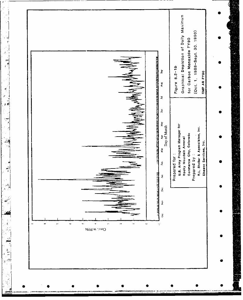
Figure 5.3-113 Graphical Depiction of Daily Maximum for Carbon Monoxide FY90 (Oct. 1,1989 - Sept. 30, 1990)

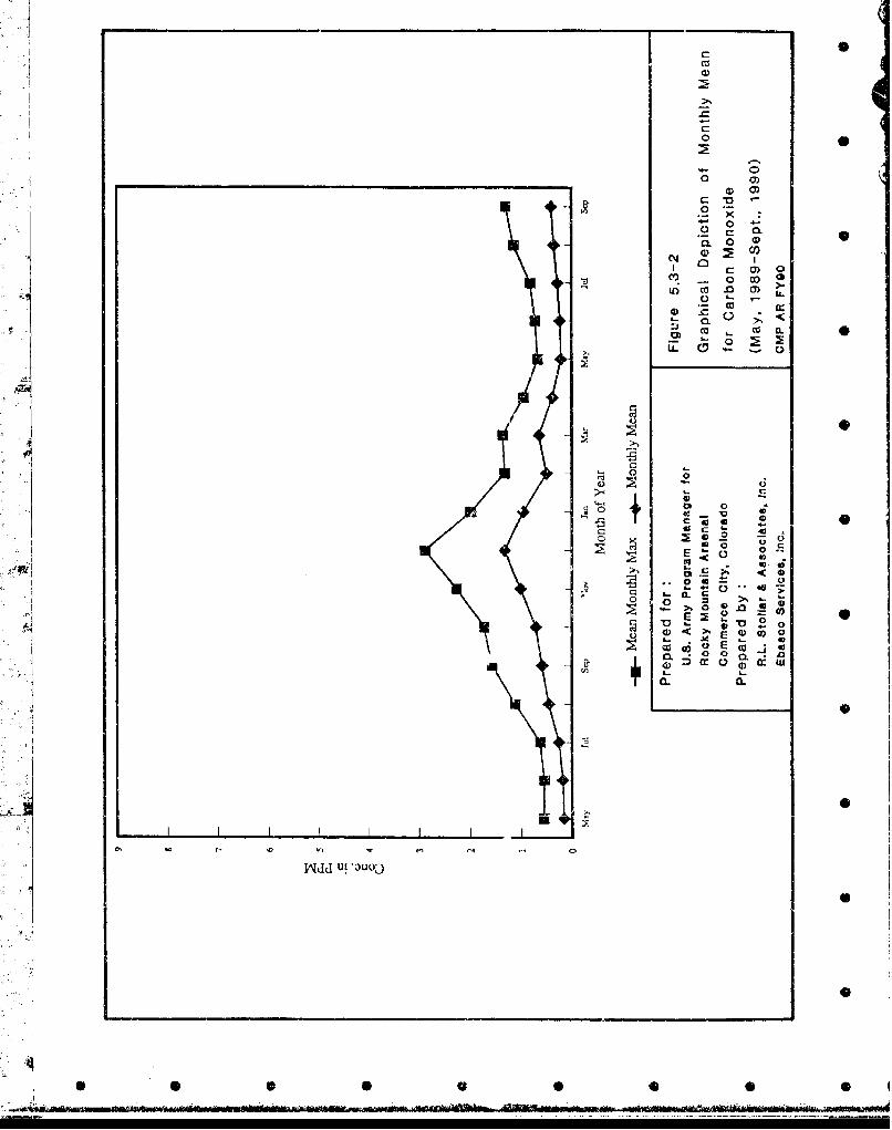
Figure 5.3-2 Graphical Depiction of Monthly Mean for Carbon Monoxide (May 1989 - Sept1990)

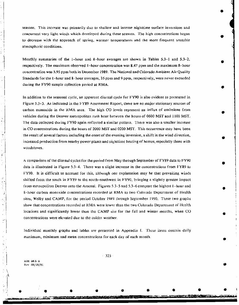
Figure 5.3-3 Graphical Depiction of Diurnal Cycle for Carbon Monoxide FY90 (Oct. 1,1989 - Sept. 30, 1990) •

Figure 5.3--4 Graphical Depiction of Diurnal Comparison f', tj bon Monoxide (MaySeptember)

Figure 5.3-5 CMP and Colorado Department of Health Siic:; ,;lu~ ';ubon MonoxidcValues (Oct. 1, 1989 - Sept. 30, 1990)

Figure 5.3-6 CMP and Colorado Department of Ilealth Sitc, , IHlum ('atbon Monoxid,Values (Oct. 1, 1989 - Sept. 30, 1990)

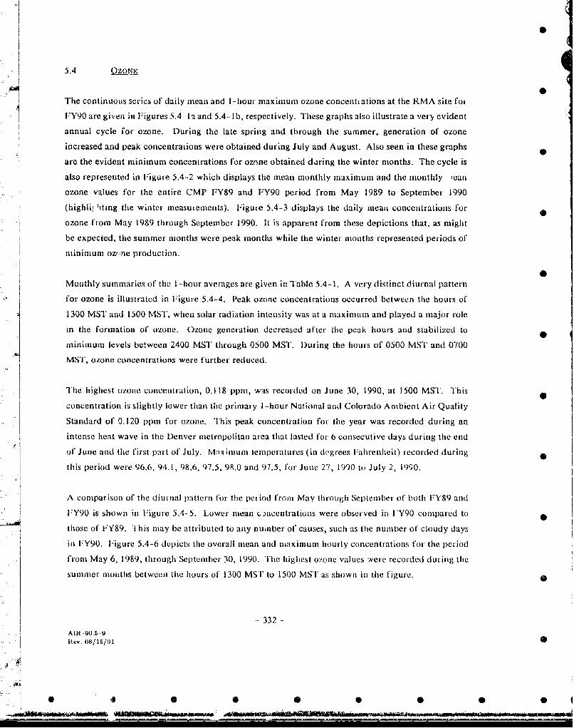
Figure 5.4--IA Graphical D)epiction of Daily Mean for Ozone FY90 (Oct. 1, 1989 - Sept. 30,1990)

Figure 5.4-IB Graphical Depiction of Daily Maximum for Ozone IY90 (Oct. I, 1989 - Sepi 0

30, 1990)

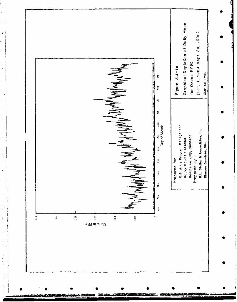
Figure 5.4-2 Graphical Depiction of Monthly Mean for Ozone (May 1989 - Sept. 1990)

Figure 5.4-3 Graphical Depiction of Daily Mean for Ozone (May 0, 1981) - Sept. 30, 1990)

Figure 5.4-4 Graphical Depiction of Diurnal Cycle for Ozone FY90 (Oct. 1, 1989 - Sept. 30,1990)

Figure 5.4-5 Graphical Depiction of Diurnal Comparison for Ozone (May -- September)

Figure 5.5-6 Graphical Depiction of Overall Mean for Ozone (May 6, 1989 - Sept. 30, 1990)

Figure 5.4-7 CMP and Colorado Department of llealth Sites 1 - Ilour Ozone Values (Oct. 1,1989 - Sept. 30, 1990)

Figure 5.5-1A Graphical Depiction of Daily Mean for Sulfur Dioxide FY90 (Oct. 1, 1989 -

Sept. 30, 1990)

Figure 5.5-1lB Graphical Depiction of Daily Maximum for Sulfur l)ioxide FY90 (Oct. 1, 1989-Sept. 30, 1990)

- xv-

AIR- 90.TO(

Rev. 08/28/91

. ". ,._ . ,,r+ tl - •i. +:'* :_ ' ' ... .. . . .'' r= --- ..... .. .z ._.... -


Figure 5.5-2 Graphical Depiction of Monthly Mean for Sulfur Dioxide (May 1989 - Sept.1990)

Figure 5.5. 3 Graphical Depiction of Daily Mean for Sulfur Dioxide (May 6, 1989 - Sept. 30,1990)

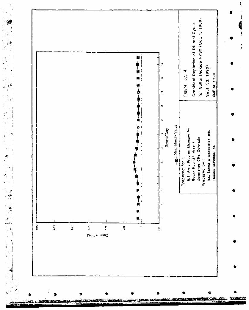
Figure 5.5-4 Graphical Depiction of Diurnal Cycle for Sulfur Dioxide FY90 (Oct. 1, 1989 - 0Sept. 30, 1990)

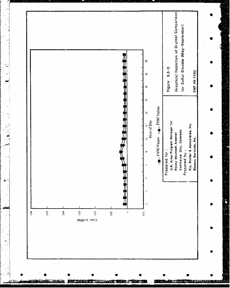
Figure 5.5-5 Graphical Depiction of Diurnal Comparison for Sulfur Dioxide (May - Sept.)

Figure 5.5-6 Graphical Depiction of Overall Mean for Sulfur Dioxide (May 6, 1989 - Sept.

30, 1990)

Figure 5.5-7 CMP and Colorado Department of Health Sites 3-Hour Sulfur Dioxide Values(Oct. 1, 1989 - Sept. 30, 1990)

Figure 5.5-8 CMP and Colorado Department of Health Sites 24-Hour Sulfur Dioxide Values(Oct. 1, 1989 - Sept. 30, 1990)

Figure 5.6-lA Graphical Depiction of Daily Mean for Nitric Oxide FY90 (Oct. 1, 1989 - Sept.30, 1990)

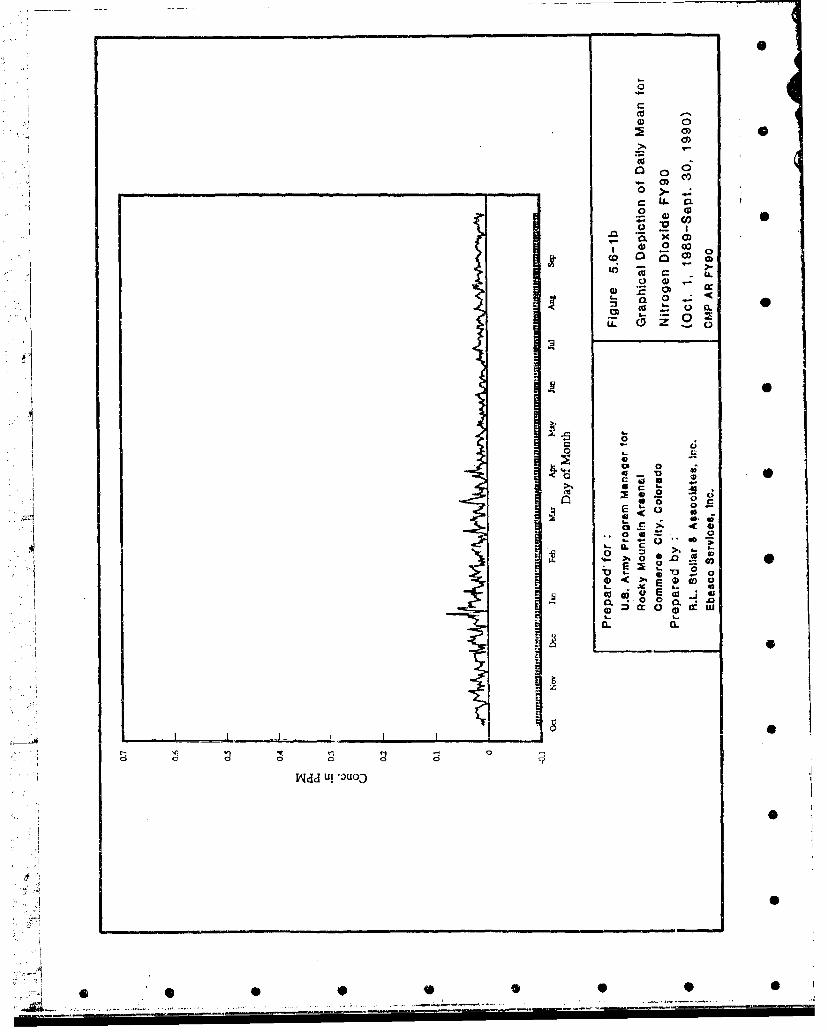
Figure 5.6- 1 B Graphical Depiction of Daily Mean for Nitrogen Dioxide FY90 (Oct- 1, 1989 -Sept. 30, 1990)

Figure 5.6--IC Graphical Depiction of Daily Mean for Nitrogen Oxides FY90 (Oct. 1, 1989 -Sept. 30, 1990)

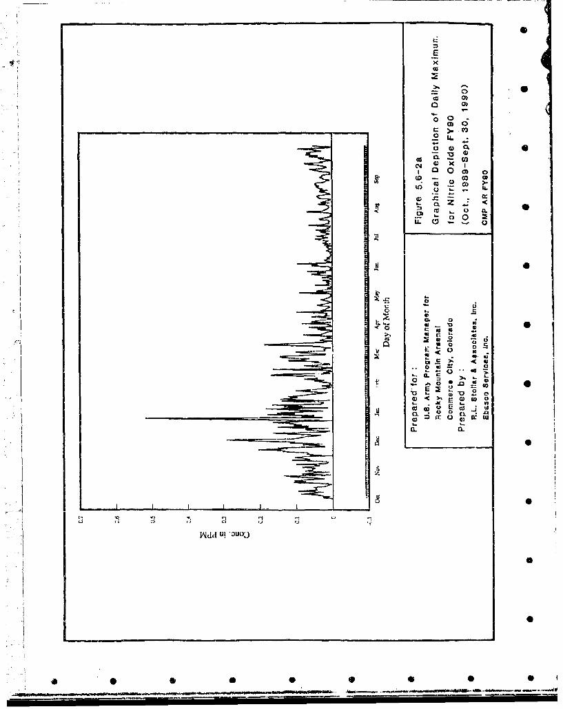
Figure 5.6-2A Graphical Depiction of Daily Maximum for Nitric Oxide FY90 (Oct. 1, 1989 -Sept. 30, 1990)

Figure 5.6-2B Graphical Depiction of Daily Maximum for Nitrogen G.ioxitdi FY90 (Oct. 1,1989 - Sept. 30, 1990)

Figure 5.6-2C Graphical Depiction of Daily Maximum for Nitrogen Oxides FY90 (Oct. 1,1989 -Sept. 30, 1990)

Figure 5.6- 3A Graphical Depiction of Monthly Mean for Nitric Oxide (May 1989 -Sept, 1990)

Figure 5.6-313 Graphical Depiction of Monthly Mean for Nitrogen l)ioxide (May 1989 -Sept.1990)

Figure 5.6-3C Graphical Depiction of Monthly Mean for Nitrogen Oxides (May 1989 -Sept.1990)

Figure 5.6-4A Graphical Depiction of Daily Mean for Nitric Oxide (May 6, 1989 -Sept. 30, 01990)

Figure 5.6-413 Graphical Depiction of Daily Mean for Nitrogen D)ioxide (May 6, 1989 -Sept.30, 1990)

Figure 5.6-4C Graphical Depiction of Daily Mean for Nitrogen Oxides (May 6, 1989 -Sept.30, 1990)

- xvi -

AItI- 90.'TJ(;

R 000ev. 08/28/91


Figure 5.6--5 Graphical Depiction of Diurnal Cycle for Nitrogen Oxides (Oct. 1, 1989 - Sept.30, 1990)

Figure 5.6-6 Graphical Depiction of Diurnal Comparison for Nitrogen Oxides (May -

September)

Figure 5.6-7 Graphical Depiction of Diurnal Mean for Nitrogen Oxides (May 6, 1989 - Sept.30, 1990)

Figure 5.6-8 CMP and Colorado Department of Health Sites 24-11our Nitroger Dioxide

Values (Oct. 1, 1989 - Sept. 30, 1990)

Figure 5.7-1 Sources of Regulated Pollutants in RMA Vicinity

Figure 5.7-2 Graphical Depiction of Carbon Monoxide for December 22-23, 1989

Figure 5.7-3 Graphical Depiction of Sulfur Dioxide for December 22-23, 1989

Figure 5.1-4 Graphical Depiction of Nitrogen Oxides for December 22-23, 1989

Figure 5.7-5 Graphical Depiction of Carbon Monoxide for May 21, 1990 0

Figure 5.7-6 Graphical Depiction of Sulfur Dioxide for May 21, 1990

:Figure 5.7-7 Graphical Depiction of Nitrog..n Oxides for May 21, 1990

Figure 6.1-1 Dust Event Case Study: May 15, 1990

Figure 6.1-2 Dust Event: May 15, 1990 (SO 2 and NO.)

Figure 6.2-1 Brown Cloud Case Study: October 25, 1990

,Figure 6.2-2 Brown Cloud Migration: October 25, 1989,

Figure 6.2-3 Brown Cloud Event: October 25, 1989 (SO2 and NO.)

Figure 6.2-4 Brown Cl)ud Event: October 25, 1989 (CO)

Figure 6.2--5 Brown Cloud Case Study: January 5, 1990

Figure 6.2-6 Brown Cloud Event: January 5, 1990 (SO, and NO.)

Figure 6.2-7 Brown Cloud Event: January 5.. 1990 (CO)

Figure 6.2-8 Brown Cloud Case Study: September 14, 1990

Figure 6.2-9 Irown Cloud Event: September 14, 1990 (SO, and NO,)

Figure 6.2- 10 Brown Cloud Evein: September i4, i990 (CO)

, Figure 7.2-I RMA Graphical Depiction of Temperature (Oct. I, 1989 - Sept 30, 1990)

Figure 7.2-2 RMA Graphical Depiction of Precipitation (Oct. I, 1989 .. Sept. 30, 1990)

Figure 7.2-3 RMA Graphical Depiction of Wind Speed and Wind Direction (Oct. 1, 1989 -Sept. 30, 1990)

AIR.-n.TO; -- xvii-

Rev. 08/28/91

A S 0- .T 0

LIST OF FIGURES (contiaued)

"Figure 7.2-4 Wind Roses for RMA (Oct. I - Dec. 20, 1989) and Stapleton Airport 1982-86 0Fall

Figure 7.2-5 Wind Roses for RMA (Dec. 21, 1989 - March 19, 1990) and Stapleton Airport1982-86 Winter

Figuie 7.2-6 Wind Roses for RMA (March 20 - June 20, 1990) and Stapleton Airport 1982-86 Spring

Figure 7.2-7 Wind roses for RMA (June 21 - Sept. 30, 1990) and Stapleton Airport 1982-86Summer

Figure 7.2-8 Wind Roses for RMA (Oct. 1, 1989 - Sept. 30, 1990) and Stapleton Airport1982-86 Annual 0

Figure 7.2-9 RMA and Stapleton Airport Fall Wind Rose Comparisons

Figure 7.2-10 RMA and Stapleton Airport Winter Wind Rose Comparisons

Figure 7.2-11 RMA and Stapleton Airport Spring Wind Rose Comparisons

Figure 7.2-12 RMA and Stapleton Airport Summer Wind Rose Comparisons

Figure 7.2-13 RMA and'Stapleton Airport Annual Wind Rose Comparisons

]0

--xvili

Ali -90.TOCRev. 08/28/91

_ _r.,,

ACRONYMS .kND ABBREVIATIONS

II ITCE I, 1, 1 -Trichlorocthane

112TCE 1, 1,2-Trichloroethane

ADI Acceptable Daily Intake

Atrazine 2-chloro-4-ethylamiino-6-isopropylamino-s-trianine

BCHPD Bicycloheptadiene 0

CA-6 Benzene

CCI4 Carbon Tetrachloride

CH 2CI2 Methylene Chloride

CiiCls Chloroform

Chlordane 1,2,4,5,6,7,8,8-octachloro-2,3,3a,4,7,7a-hexahydro-.4,7--methano-111-indene

CICIH 5 Chlorobenzene

CMP FY90 Comprehensive Monitoring Program Fiscal Year 1990

CO Carbon Monoxide

CRL Certified Reporting Limit

DBCP Dibromochioropropane

DCLEI 1 1,1 - Dichloroethane

DCLE12 1,2-DichloroctlhaneDCPD Dicyclopentadiene

DDD Dichlorodiphenyldichioroethane

.)MII12 Dimethylbenzene

4 DMDS I)imethyl Disulfidc

EPA Environmental Protection Agency

ETCrI15 Ethylbcnzene

GC/MS Gas Chromatography/Mass Spectrometry

GC/ECD Gas Chromatography/Electron Capture Detection

ICAP Inductively Coupled Argon Plasma

Malathion 0,0.-.dimethyl-s-(1,2-dicarboxyethyl) phosphorodithioate

MEC6tlb Toluene

MIBK Methyl isobutyl Ketone

NIST Mountain Standard Time

NAAQS National Ambient Air Quality Standards 0

NATICII National Air Toxics Information ClearinghouseN IOSH National Institute of Occupational Safety and Iealth

NNDME A N-Nitrosodimethylamine

NO, Nitrogen Oxides 0

Os Ozone

-- xixALR- 9(.TO(C

11ev. 08/28/9I

40 0 0 00.....d

ACRONYMS AND ABBREVIATIONS (continued)

OCP Organochlorine Pesticides

Parathion Parathion (C1 oH 14NO5 PS)

PMRMA Program Manager Rocky Mountain Arsenal

PM-10 Respirable Particulates less than 10 microns

PPDDE Dichlorodiphenylethane 0

PPDDT Dichlorodiphenyltrichloroethane

SO 2 Sulfur Dioxide

Supona 2-clioro- l-(2,4-dichlorophenyl) vinyl diethyl phosphate

SVOC Semi-Volatile Organic Compounds

TI2DCE Trans-- 1,2--Dichloroethene 0

TCLEE Tetrachloroethene

TLV threshold limit value

tpy tons per year

TRCLE Trichloroethene

TSP Total Suspended Particulates

USATHAMA U.S. Army Toxic and Hazardous Materials Agency

USAEIIA U.S. Army Environmental Hygiene Agency

VOC Volatile Organic Compounds

XYLENE Xylene

0

XX

* AIR *90).''oCi .v,. 08/28u/91 0

.0 0 0 0 S 0 0 S 4

0

5.0 CONTINUOUS AIR MONITORING PROGRAM

O5.1 PROGRAM OVERVIEW

The Continuous Air Monitoring Program is described in Section 3.6. Measurements of criteria

gaseous pollutants were taken continuously, and recorded automatically in a data acquisition system.

The hourly averages of the sampling data for carbon monoxide (CO), ozone (Os), sulfur dioxide (SO 2),

nitric oxide (NO), nitrogen dioxide (NO.) and nitrogen oxides (NO,) are presented in Appendix I for

the period October 1, 1989, through September 30, 1990, and are summarized in this section. A

description of the regional atmospheric characteristics of these gases is found in Sections 2.1.3 through

2 i.6.

The purpose of the gaseous monitoring program was to identify background concentrations ofpollutants which play a role in possible future remediation activities. An assessment of these datayields additional insight into the atmospheric characteristics in and around the RMA site. It provides

a general overview of the gaseous concentrations, as well as highlighting any anomalous values. Theanalysis also helps to identify meteorological and dispersion conditions which may effect air quality

at RMA. For example, frequently occu:rring diurnal drainage wind pattern with a south to north air

flow at night and a north to south air flow during the day affects all six gas concentrations lo some

extent. Diurnal drainage winds are described in more detail in Section 2.2. Daytime photochemical

activity primarily influences O and NO 2. A summary of average and I-hour maximum

concen-trations as measured during the FY90 program, as well as additional analyses, is provided in

this section.

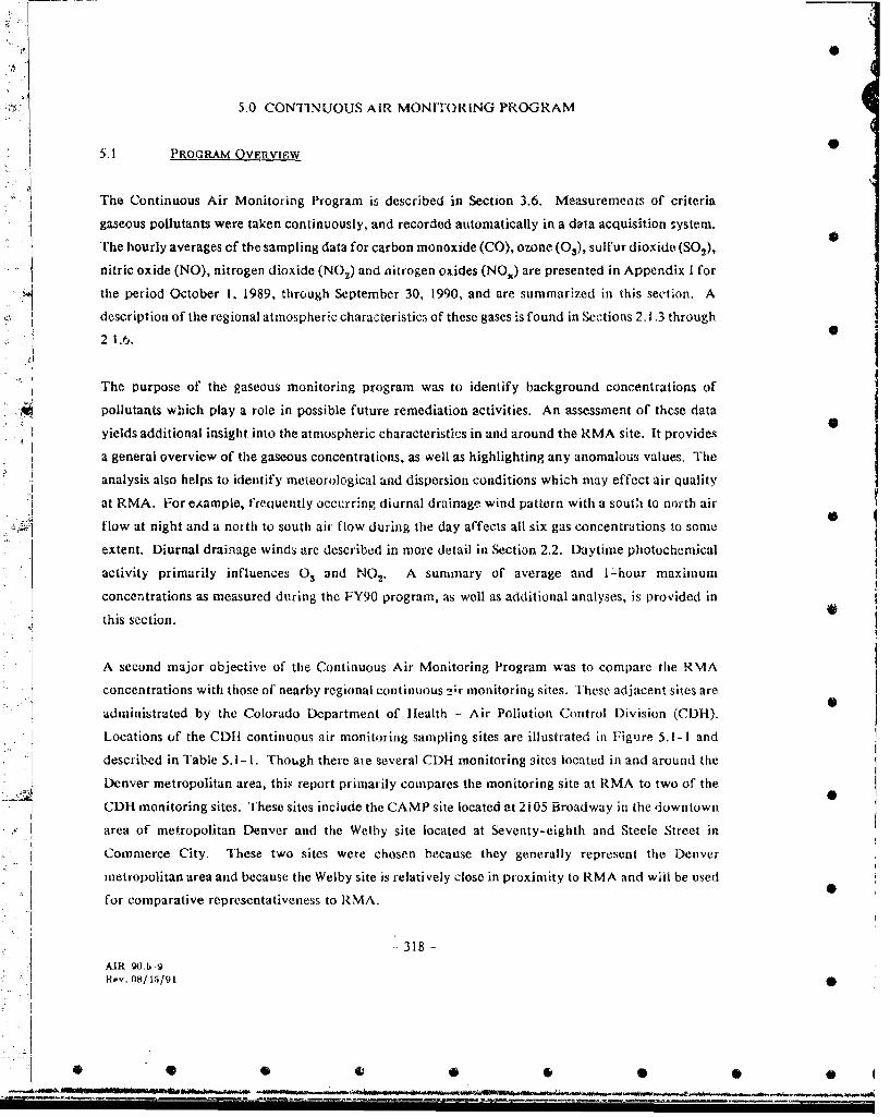
A second major objective of the Continuous Air Monitoring Program was to compare tlhe RMA

concentrations with those of nearby regional continuous !!;r monitoring sites. These adjacent sites are

"administrated by the Colorado Department of Hlealth - Air Pollution Control Division (CDIl).

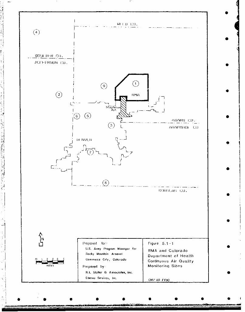
Locations of the CDH continuous air monitoring sampling sites are illustrated in Figure 5.1-1 and

described in Table 5.1-i. Though there aie several CDH monitoring sites located in and around the

Denver metropolitan area, this report primarily compares the monitoring site at RMA to two of the

CDHimonitoringsites. These sites include the CAMP site located at 2i05 Broadway in the downtown

area of metropolitan Denver and the Welby site located at Seventy-eighth and Steele Street in

Commerce City. These two sites were chosen because they generally represent the Denver

metropolitan area and because the Welby site is relatively close in proximity to RMA and will be used

for comparative representativeness to RMA.

318 -

AIRe-.0/.5 -9w~v. 08/15/91 0

A"1W1 1 1) (().

JILUFRSUN L:O.T

S...... .L/'' "- - -' 1:.1Apl..f.

. "'Ii _

IdL

I

DI) NVI4 ,1

iLL

KL ._ Q- -.

@.

2t_. :1

iS

Prepared for: Figure 5.1-1

U.S. Army Program Manager for RMA and ColoradoRocky Mountain Arsenal Department of HealthCommerce City, Colorado Continuous Air Quality

,L5 Prepared by: Monitoring Sites

R.L Stoltar a Associates, Inc. SEboaco ServicOe, Inc. CMP AR FY90

S 0 m0 .....

. ..

. -. . .S, 0 ._

•• -- --. _ ..= - . '

Table 5.1-1 RMA and Colorado Department of Health Gaseour Emissions Monitoring Sites

Repor.6d Parameters _

Site Site Site I I I INumber Name Address CO 03 SO2 NO N02 NOX

I RMA 8th Avenue at D Street X X X X X X

2 Arvada 57th at Garrison

3 Albion 14th at Albion

4 Boulder 2320 Marine

5 Camp 2105 Broadway X X X X 6

6 Carriage 23rd and Julian X X

7 Englewood 3300 South Huron X X

8 Highland 8100 South University X X I

9 Welby 78th at Steele X X X x

0

L0

4.

AIR-TBLI.90

* 00 0 0 0 0 06 4

The Continuous Air Monitoring Program serves to establish baseline levels of gaseous constituents for

future air quality assessments. Measured concentrations can be compared with various meteorological

data such as . ind direction and stability to identify possible migration patterns of gaseous pollutants

from metropolitan Denver onto RMA. Also, baseline levels may be used to predict the impact a

SfuLure remedial activity source may have on the environment. The results shown here represent a

complete year of data collection and an assessment of diurnal and annual cycles of each gas.

5.2 ANALYSIS OVERVIEW

A variety of tables and graphs were used to summarize the continuous air quality data. Mean values

refer to daily averages and the 1-hour maximum value refers to the highest 1-hour average value

recorded daily. Comparisons of RMA data were made with National Ambient Air Quality Standards

(NAAQS) as well as with data from Colorado Department of Health sites. A further comparison was

made for the data collection period of May through September for CMP FY89 and the current CMP

"FY90 data. The analyses for carbon monoxide, ozone, and sulfur dioxide are presented individually

in the following subsections. For nitric oxide, nitrogen dioxide, and nitrogen oxides, a combined

analyses is provided because of the similarities in their chemical composition and concentration

characteristics. Case studies were presented to examine the possible sources of some of the higher

concentrations observed at RMA.

5.3 A&RBON MONOXIDE

The series of daily mean arid l-h'ur maximum carbon monoxide concentrations are illustrated in

Figures 5.3-la and 5.3-lb, respectively. During the sample collection period for FY90, there were

a number of occasions where the daily maximum was several times greater than the daily average.

Also for this pei iod, there were several occasions where the daily maximum and the daily mean were

nearly the same value. Such instances usually occurred when persistent winds were blowing with a

nu, therly component or a southeasterly component. This flow allowed industrial pollutant matter to

migrate away from RMA and thus not be detected.

Figures 5.3-la and 5.3-lb depict the continuous annual cycle of CO values for RMA which is

basically a rerlection of the Denver metropolitan area. This cycle is also illustrated for, mean monthly

maximum and monthly mean values Tor the entire CMP FY89 and FY90 monitorng period from May

1989 to September 1990 in Figure 5.3-2. Evident in these graphs is the gradual increase in the daily

mean, and mean monthly maximum and monthly mean concentrations during the fall and winter

- 321 -

AIR-90.5-9Rev. 08/15/91 6

S ._ -S S7S

0 C

0

0)

0)

u 00

- 1 0 0 C2

0 0 >

Wý w

,~ J7

-d Cu'UO-

ES

J~EEx

00 )Cu )

C L

00 o

t . o~-

0 0 O

S 0

0

w aoILO 0 m m )

, 0 .

co 0

U .2

03 .±93

0- 0 'n

cI 0 LCýl

WdI 0t -a

fbt

seasons. This increase was primarily due to shallow and intense nighttime surface inversions and

concurrent very light winds which developed during these seasons. The high concentrations began

to decrease with the approach of spring, warmer temperatures and the more frequent unstable

atmospheric conditions.

Monthly summaries of the 1-hour and 8-hour averages are shown in Tables 5.3-1 and 5.3-2,

respectively. The maximum observed I-hour concentration was 8.47 ppm and the maximum 8-hour

concentration was 5.95 ppm both in December 1989. The National and Colorado Ambient Air Quality

Standards for the I-hour and 8-hour averages, 35 ppm and 9 ppm, respectively, were never exceeded

during the FY90 sample collection period at RMA.

In addition to the seasonal cycle, an apparent diurnal cycle for FY90 is also evident as presented in

Figure 5.3-3. As indicated in the FY89 Assessment Report, there are no major stationary sources of

carbon monoxide in the RMA area. The high CO levels represent an influx of emissions from 0vehicles during the Denver metropolitan rush hour between the hours of 0600 MST and 1100 MST.

The data collected during FY90 again reflected a similar pattern. There was also a smaller increase

in CO concentrations during the hours of 2000 MST and 0200 MST. This occurrence may have been

the result of several factors including the onset of the evening inversion, a shift in the wind direction,

increased production from nearby power plants and righttime heating of homes, especially those with

woodstoves.

A comparison of the diurnal cycles for the period from May through September of FY89 data to FY90

data is illustrated in Figure 5.3-4. There was a slight increase in the concentrations from FY89 to

FY90. It is difficult to account for this, although one explanation may be that prevailing winds

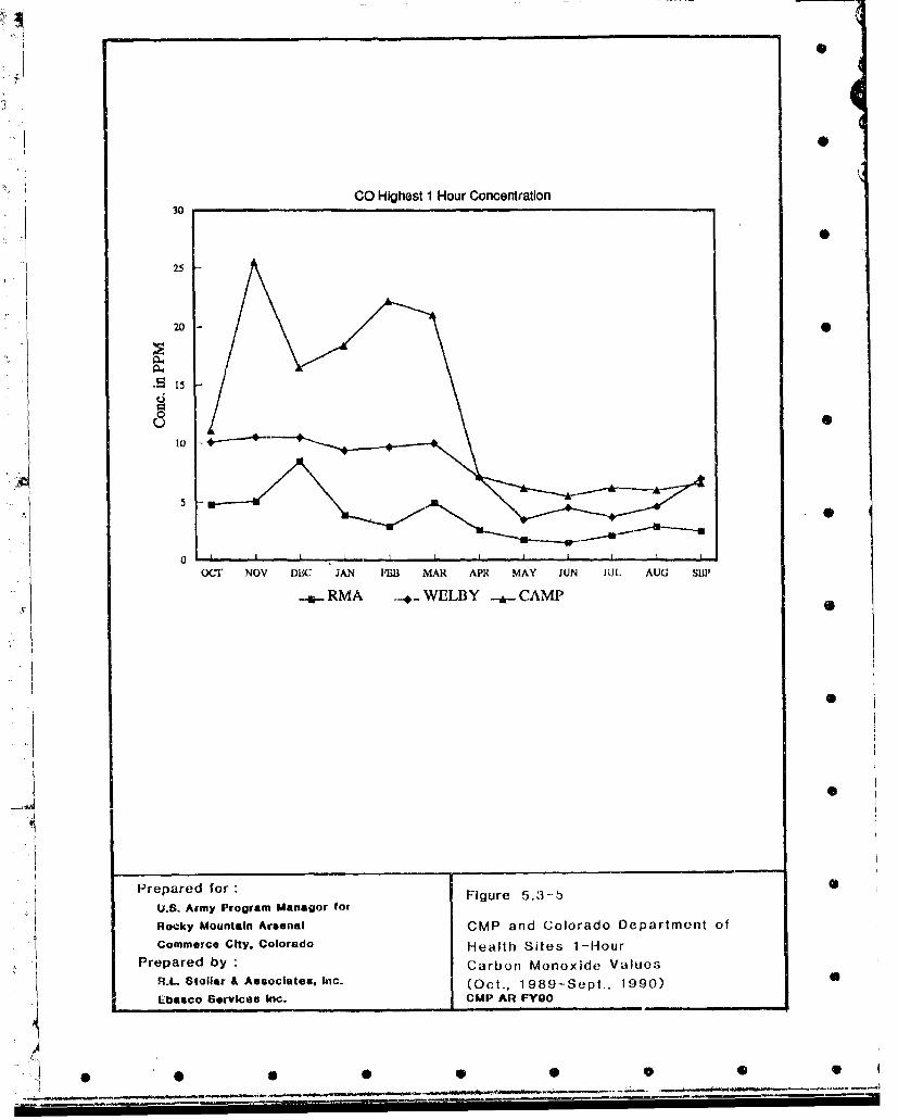
shifted from the south in FY89 to the south-southwest in FY90, bringing a slightly greater impact

from metropolitan Denver onto the Arsenal. Figures 5.3-5 and 5.3-6 compare the highest I-hour and

8-hour carbon monoxide concentrations recorded at RMA to two Colorado Department of Health

sites, Welby and CAMP, for the period October 1989 through September 1990. These two graphs

show that concentrations recorded at RMA were lower than the two Colorado Department of Ilealth

locations and significantly lower than the CAMP site for the fall and winter months, when CO

concentrations were elevated due to the colder weather.

Individual monthly graphs and tables are presented in Appendix 1. These items contain daily

maximum, minimum and mean concentrations for each day of each month.

- 325 -

AIR 90.5-9Rev. 08/15/91

..........

* 0 6L'-• • - 0 0 .......... 0 0t--" 0'--. .

0

Table 5.3-1 Summary of Carbon Mozvoxide I-Hour Average Values in ppm1 October, 1, 1989(0100 MST) through September 30, 1990 (2400 MST)

Oct Nov Dec Jan Feb Mar

Mean 0.71 1.00 1.36 0.96 0.50 0.640

Maximum 4.83 5.07 8.47 3.88 2.91 4.97

2nd Highest Maximum 3.86 3.95 7.74 3.75 2.67 4.32

Minimum 0.23 0.49 0.73 0.10 0.10 0.100

Apr May Jun Jul Aug Sep

Mean 0.39 0.21 0.23 0.28 0.35 0.40 0

Maximum 2.57 1.77 1.49 2.10 2.90 2.52

2nd hlighest Maximum 2.01 1.65 1.48 1.80 1.77 2.39

Minimum 0.10 0.10 0.10 0.10 0.10 0.10S

Mean for Entire Period 0.60

Federal and Colorado Ambient Air Quality Standard for maximum I-hour average values is35 ppm, not to be exceeded more than once a year. 40

0

':AIR-Ti3L1.90 O

"UUUU

Table 5.3-2 Summary of Carbon Monoxide 8-Htour Average Values in ppm1 October, 1, 1989- (0100 MST) through September 30, 1990 (2400 MST)


Mean 0.71 1.00 1.36 0.96 0.50 0.64

Maximum 2.29 2.98 5.95 2.78 1.88 3.66


Minimum 0.25 0.54 0.76 0.10 0.10 0.100


Mean 0.39 0.21 0.23 0.28 0.35 0.40 0

Maximum 1.21 1.09 0.88 1.37 1.05 1.52


Minimum 0.10 0.10 0.10 0.10 0.10 0.10


Federal and Colorado Ambient Air Quality Standard for maximum 8-hour average values is9 ppm, not to be exceeded more than once a year.

S~0

>1 0

AIR rBL1.A9 0j:

S. w

.2.CL0

0

-w 0

.0

C J

-a I L

Wdd UT 'O0

-x

(U0

3 ~~00

C?

Lc l0

000

W 0 o

o0

:2 00r L. 0

00 0-

Wc' -l .010L

0

CO Highest I Hour Concentration30

0

25

20 0

.iI15

101,O(Y' NOV DBC JAN i13 MAR AIR MAY JUN JUL AUG SIWI

-. RMA - WELBY &- CAMP


U.S. Army Program Managor for

Rocky Mountain Arsenal CMP and Colorado Department of

Commerce City. Colorado Health Sites 1-Hour

Prepared by : Carbon Monoxide Values

RAL Stollar A Associates. Inc. (Oct., 1989-Sept., 1990)

Ebasco Services Inc. CMP AR FY00

S0 , 0 •0 0 0

CO Highest 8 Hour Concentration14

12

10

4

=2

0 1 1OC' NOV DUC JAN FEB1 MAR APR MAY JUN JU1, AUG SF.I

- RMA -#- WE ,1BY . CAMP S

I6

Prepared for Figure 5.3-6U.S. Army Program Manager for

Rocky Mountain Arsenal CMP and Colorado Department ofCommerce City. Colorado Health Sites 8-Hour

Prepared by Carbon Monoxide Values

R.L Stollar & Aasociatas, Inc. (Oct., 1989-Sept., 1990)

Ebasco Gervy-8s Inc. CMP AR FYGO

0 0~~~= S -

5.4 QZONE

The continuous series of daily mean and I -hour maximum ozone concentrations at the RMA site for

FY90 are given 'n Figures 5.4- Ia and 5.4- I b, respectively. These graphs also illustrate a very evident

annual cycle for ozone. During the late spring and through the summer, generation of ozone

increased and peak concentrations were obtained during July and August. Also seen in these graphs

are the evident minimum concentrations for oz.ne obtained daring the winter months. The cycle is

also represented in Figure 5.4-2 which displays the mean monthly maximum and the monthly 'can

ozone values for the entire CMP FY89 and FY90 period from May 1989 to September 1990

(highli! lfting the winter measurements). Figure 5.4-3 displays the daily mean concentrations for

ozone from May 1989 through September 1990. It is apparent from these depictions that, as might

be expected, the summer months were peak months while the winter months represented periods of

minimum oz(.ne production.

Monthly summaries of the 1-hour averages are given in Table 5.4-1. A very distinct diurnal pattern

for ozone is illustrated in F~igure 5.4-4. Peak ozone concentrations occurred between the hours of

1300 MST and 1500 MST, when solar radiation intensity was at a maximum and played a major role

in the formation of ozone. Ozone generation decreased after the peak hours and stabilized to

minimum levels between 2400 MST through 0500 MST. During tile hours of 0500 MST and 0700

MST, ozone concentrations were further reduced.

The highest ozone concentration, 0.118 ppm, wais recorded on June 30, 1990, at 1500 MST. This

concentration is slightly lower than the primary I-hour National and Colorado Ambient Air Quality

Standard of 0.120 ppm for ozone. This peak concentration for the year was recorded during an

intense heat wave in the Denver metropolitan area that lasted for 6 consecutive days during the end

of June and the first part of July. Maximum temperatures (in d(grees Iahrenheit) recorded during

this period were 96.6, 94.1, 98.6, 97.5, 98.0 and 97.5, for June 27, 1990 to July 2, 1990.

A comparison of the diurnal pattern for the period from May through September of both FY89 and

FY90 is shown in Figure 5.4-5. Lower mean cjncentrations were observed in FY90 compared to

those of 1:Y89. 1his may be attributed to any number of causes, such as the number of cloudy days

in FY90. Figure 5.4-0 depicts the overall mean and maximum hourly concentrations for the period

from May 6, 1989, through September 30, 1990. The highest ozone values were recorded during the

summer months between the hours of 1300 MST to 1500 MST as shown in the figure.

332 -

AIR -90.5 -0Rev. 018/1/91 0

A

00

00

Q 00)

:U03

0

Ch-

40

0)(U 0.

(I co~

.... ... I'd.~~~ .- .~ .0 ..... o k

E

0

0Y)

C, • 0

,5 •o a.•o•9 "~ 0

0.0

LLLX

.. . go

E= 2

.e

S:co 0

E j

0.0

00-

.. ..

.. ... • .•_0....•• .

. . ...

i ""J... U I n I u n, ,•

0

- CL

0)

I 0 0)

CL 0.0 >

a 0

40-

*- 0 c

0 *Ia~ ~' E~E00

cUL

14@~i

UT6.Wdd 0..)U

CL

CD 0) C

0 Z:

CL- 0 0

o

a 0 CL

:i) Ci C

CL 0

ci6KI cul':w OD

" Nv'0MM

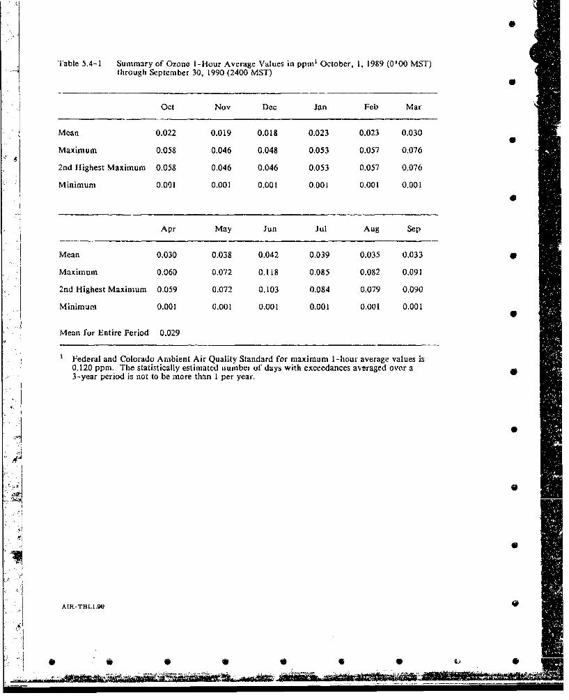
Table 5.4-1 Summary of Ozone I-Hour Average Values in ppm1 October, i, 1989 (0100 MST)through September 30, 1990 (2400 MST)

0


Moan 0.022 0.019 0.018 0.023 0.023 0.030M u 02nd Highest Maximum 0.058 0.046 0.046 0.053 0.057 0.0762dHgetMaximum 0.058 0.046 0.046 0.053 0.057 0.076

Minimum 0.001 0.001 0.001 0.001 0.001 0.0010


Mean 0.030 0.038 0.042 0.039 0.035 0.033 0

Maximum 0.060 0.072 0.118 0.085 0.082 0.091

2nd Highest Maximum 0U059 0.072 0.103 0.084 0.079 0.090

Minimum 0.001 0.001 0.001 0.001 0.001 0.001


1Federal and Colorado Ambient Air Quality Standard for maximum I-hour average values is0.120 ppm. The statistically estimated number of days with exceedances averaged over a3-year period is not to be more than 1 per year.

4 0i

0

AIR-TBLIO0

!!14

. . . . . . .I

L 00

(3)

0 .0 L

C CL

as)

00

,- a0

20 E docl 0 0 0.

4 ) cc >0)i L

ro~ 0P rvim -- ---

00

a4

0

o0

LO 0 -I rI D

'I 0 a 0CO Co ~

U- -00~~

000

0

o .() , *

0. ~ :0 o~ ~~ (

AC L

uu

Wdo U! 0 a D

Cl) -

0l

00

00 -

0 cc

0) - )

0a

00

Cx 0a: 0 0u

4u s

'C C

Ki U 'O' H

0 a a dfde V0

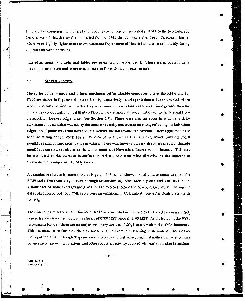
Figure 5.4-7 compares the highest I -hour ozone concentratioois recorded at RMA to the two Colorado

Department of Health sites for the period October 1989 through September 1990. Concentrations at

RMA were slightly higher than the two Colorado Department of Health locations, most notably during

#, the fall and winter seasons.

Individual monthly graphs and tables are presented in Appendix I. These items contain daily

maximum, minimum and mean concentrations for each day of each month.

5.5 SULFLUR DIoxU•ŽU

The series of daily mean and I-hour maximum sulfur dioxide concentrations at the RMA site for

FY90 are shown in Figures 5.5- ia and 5.5- Ib, respectively. During this data collection period, there

were numerous occasions where the daily maximum concentration was several times greater thtan the

daily mean concentration, most likely reflecting the transport of concentrations onto the Arsenal from

metropolitan Denver SO, sources (see Section 5.7). There were also instances in which the daily

maximum concentration was nearly the same as the daily mean concentration, reflecting periods when

migration of pollutants from metropolitan Denver was not toward the Arsenal. There appears to have

been no strong annual cycle for sulfur dioxide as shown in Figure 5.5-2, which provides mean

monthly maximum and monthly mean values. There was, however, a very slight rise in sulfur dioxide

monthly mean concentrations for the winter months of November, December and January. This may

be attributed to the increase in surface inversions, persistent wind direction or the increase in

emissions from major nearby SO 2 sources

4

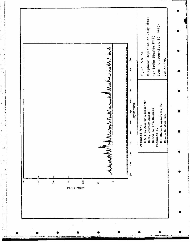
A cumulative picture is represented in IFiguiý 5.5-3, which shows the daily mean concentrations for

FY89 and FY90 from May u, 1989, through September 30, 1990. Monthly summaries of the I-hour,

3-.hour and 24-hour averages are given in Tables 5.5-1, 5.5-2 and 5.5-3, respectively. During the

data collection period for FY90, thee were no violations of Colorado Ambient Air Quality Standards

I for SO 2.

'The diurnal pattern for sulfur dioxide at RMA is illustrated in Figure 5.5-4. A slight increase in SO2

concentrations is evident during the hours of 0700 MST through 1100 MST. As indicated in the FY89

Assessment Report, there are no major stationary sources of SO2 located within the RMA boundary.

This increase in sulfur dioxide may have result,-d from the morning rush hour of the Denver

metropolitan area, although SO 2 emissions from vehicle traffic are small. Another explanation may 0

be increased power generations and other industrial act*vity coupled with early morning inversions.

- 341 -

SAIR-go.5 -9

"R"v. ,t8/15/91 S

4 0 0 0 0 0 U

0

03 Highest 1 Hour Concentration0.13

0.12

0.11 -

0.10

0.09

0.080. 0.08 ;-

0.07 -

0.06 -

0.05

0.0430 ' 03o

OCT NOV DEC JAN MWJ MAR APR MAY JUN JUL AUG SHP

.-- RMA -.- WELBY . CAMP S

Prepared for: SU.S. Army Program Manager for Figure 5.4-7

Rocky Mountain Arsenal CMP and Colorado Department of

Commerce City, Colorado Health Sites 1 -Hour

riepared by Ozone Values

,1R.L. Stoller & Assoclates, Inc. (Oct., 1989-Sept., 1990) S

"Ebasco Services Inc. CMP AR FY90

S S: S . . ... .. ...

0 0c

__ _c LL -

(o- )0

0

43 00 00

ID

1% 0) 0

-a 0 0< >. 4, 0. ) a.

L 0 0 CL

0 -

=sw> 0)

L41 00

>.o m-0

clx

-j _.-f -- - - ------

C)0

0 m

C 0

o)c

00

Do 00

00

10 - (. 02 .

CL 0 ) -

U- (DD-- c

CL (

6 6 4y

Wd * O1

cdI0

0 •

C.4 - CO

x I

10

•d 2, uo

04 0

0 w

ic

Wd UTUOO

. •...... --.. .. .. ..... •. "'ll,

S

Table 5.5-1 Summary of Sulfur Dioxide I-Hour Average Values in ppm1 October, 1, 1989(0100 MST) through September 30, 1990 (2400 MST)


Mean 0.002 0 002 0.003 0.002 0.002 0.0020

Maximum 0.027 0.018 0.027 0.037 0.029 0.038


Minimum 0.001 0.001 0.001 0.001 0.001 0.001


Mean 0.001 0.001 0.001 0.001 0.002 0.002

Maximum 0.026 0.051 0.038 0.018 0.042 0.038


Minimum 0.001 0.001 0.001 0.001 0.001 0.0010


National and Colorado Ambient Air Quality Standard for annual arithmetic mean is 0.030 ppm.

(There is no NAAQ 1-hour standard for SO..)

0

AIR-TBIL1.90 S

S 0 0 0 0 0 S 0 5 • 4

Table 5.5-2 Summary of Sulfur Dioxide 3-Hour Average Values in ppm1 October, 1, 1989(0100 M3ST) through September 30, 1990 (2400 MST)


Mean 0.002 0.002 0.003 0.002 0.002 0.002 0

Maximum 0.016 0.018 0.024 0.030 0.022 0.020

2nd Highest Maximum 0.015 0,017 0.022 0.027 0.018 0.018

Minimum 0.001 0,001 0.001 0.001 0.001 0.001S


Mean 0.002 0.002 0.002 0.002 0.002 0.002 S

Maximum 0.020 0.029 0.020 0.012 0.029 0.028

2nd Highest Maximum 0,017 0.028 0.020 0.012 0.022 0.036

Minimum 0.001 0.001 0.001 0.001 0.001 0.001


' Federal and Colorado Ambient Air Quality Standard for maximum 3-hour average values is0.500 ppm, not to be exceeded mos-e than once per year.

40

Al FL-TBI1.9O

-. .. ..........

jTF0

Table 5.5-3 Sumn-ary of Sulfur Dioxide 24-Hour Average Values in ppm1 October, 1, 1989(0100 MST) through September 30, 1990 (2400 MST)

]Oct Nov Dec Jan Feb Mar

Mean 0.002 0.002 0.003 0,002 0.002 0.002

Maximum 0.006 0.006 0.010 0.021 0.005 0.006


Minimum 0.001 0.001 0.00 1 0.00 1 0.001 0,001


Mean 0.002 0.002 0.002 0.002 0.002 0.002

Maximum 0.00j 0.008 0.006 0.004 0.009 0.006

2nd Highest Maximum 0.004 0,008 0.006 0.004 0.009 0.005

Minimum 0.001 0.001 0.001 0.001 0.001 0.001

Mean fo. Entire Period 0.002

1Federal and Colorado Ambient Air Quality Standard for maximum 24-hour average values is0.140 ppm, not to be exceeded more than once per year.

AIR-TBLI.9C3

cS

0)0

CD

CLLL

00

4D a

2 0--

0

0 0 C0

a. 0

14U 1

"A comparison of the diurnal patterns for the period from May through September for FY89 and FY90

is shown in Figure 5.5-5. This graph shows a slight increase in the overall FY90 diurnal pattern when

compared to FY89, although this pattern may be attributable to the fact that FY89 data included only

the May-September values.

An overall diurnal pattern for the extended period May 6, 1989, through September 30, 1990, and the

overall maximum concentrations for each hour during the same period is depicted in Figure 5.5-6.

Peak concentrations occui red at varying periods during the day, reflecting inversion conditions, wind

flow patterns and source emissions for individual events. One such event, a maximum SO 2

concentration of 0.051 ppm measured at 0X00 MST on May 21, 1990, is discussed in the case study

examples provided in Section 5.7.

Figures 5.5-7 and 5.5-8 compare the highest 3-hour and 24-hoe- sulfur dioxide concentrations

recorded at RMA to two Colorado Department of Health sites for the period October 1989 through

September 1990. The RMA site recorded lower values than the two Colorado Department of Health

sites, and considerably smaller values than at the CAMP location.

Individual monthly graphs and tables are presented in Appendix 1. These itemns contain daily

. maximum, minimum and mean concentrations for each day of each month.

5.6 NITRIC OXIE. NWrITROGEN DIOXIDE AND NiTROGFN .XIDE'S

S

Nitric oxide (NO), nitrogen dioxide (NO 2) and nitrogen oxides (NO.) data exhibited similar patterns

through the data collection period for FY90. This is supported by the following: 1) NO and NO 2

have similar sources and removal mechanisms, and 2) the concentration of NO, is the sum of NO and

NO 2 concentrations.

The series of daily mean concentrations for NO, NO 2 and NO. are shown in Figures 5.6-la, 5.6-lb

and 5.6-1c, respectively. The series of daily maximum concentrations for NO, NO 2 and NO. are

shown in Figures 5.6-2a, 5.6-2b and 5.6-2c, respectively. These graphs show an annual cycle for each

parameter with oeak concentrations most prevalont during the winter months of November, December

and January. There were predominant increases in the concentrations during this 3-month period.

This cycle is further illustrated in Figures 5.6-3a, 5.6-3b and 5.6-3c which display mean monthlyrivmximum and monthly mean concent.,ations for the complete CMP cumulative annual cycle from May

6, 1989, through September 30, 1990. This is also shown in Figures 5.6-4a, 5.6..4b and 5.6-4c, which

351 -

Rev. 08/15/91 S

. '' III

0

co0

E

00r-

cJ

a.*-0

000

E 2

I') 0)0x CL .

4.1.1

A 4&-

7a.TC

!S

0 C

0

"

L6 i .0

B 6

4- 0

' a.

I

IL

E :2Z0

iL

(0wc0

-n n , ,l

S02 Highest 3 Hour Conc-entratin0.14

0.12

0.12

.40.08

kS006

0.04

0.02

00

Prepared for:Fgr .-U.S. Army Program Manager for Fgr .-Rocky Mountain Arsenal CMP and Colorado Department of

Commerce City. ColoradoHalhSts-ouPrepared by Sulfur Dioxido Values

A.L Stollar & Associates. Inc. (c* 09Sp. 90Ebasco Services Inc. CMP AC, F900

fsB

802 HigIheat 24 Hour Concentratin0.14

* 0.12

0.1-

0.0.08-

~0.06

0,04-

0.02

0.0

OCI' NOV OLIC JAN M~U MAR AIR MAY JUN JUL AUG SUP

~-RMA *WELBY ~.CAMP

Prepared for: iue 55'

U.S. Army Program Manager for

Rocky Mountain Arsonal CMVP and Colorado Departmnent ofCommerce City. Colorado Health Sites 24-1-our

Prepared by Sulfur Dioxide Values.L. Stoliar & Associates. inc. (Oct., 1989--Sept., 1990)0

Et .-00 '.1vic-es Inc. CMIP AR IFY90

y' .1

0 l

CL

a

E4 0 0C

0 m (

E 1- 0 0

oO E CO

ca o. E

0 0 C3 t

-l1 ,.

.+.!

°'! • "-o " d

• U

L. . I..•~~I- I..0. 0...

a .-- I,,I.*-"I I I I I °I4$ C o -' g •

C 0 0 0

V'dd.Ut •UQ3• • •0

S+:.: • • •' • •.0' 4'• ,

S 0 S 0 ',- 0 0

CD

400

~ ~co co*~ o

1CO

EU C .a(30.-

u* -O 0) )

0)

U;I

m 0 IL

m 0)

co 0

0.

ii~~ ,, ,•0 t• "0000 C.

W .

E (D 0

0 m

U ;. ,.@

• -i -

S•{ Ndd ul "Ouo3

.. . .

0o.-. o.

...

I • @@ I0ii%• .• ..... i:'n .... i-r i ...... r- -'-"r r • ... :i '- : .. • ....a

L

EV x

co 0)0 0)

ow 0

CM, 0

I a0Q ) m

U)

0- -0 C

0 0 2

C6 0

V0

A:ý 0E6

.. 3

0 j

a 0, lCD

'I g ii.ltWad~~a II o(L

E

2

x

o 0)>- LL

0 -

0)

-~C) 0 CL

I r- I( 0 00) 0)

02 .C >

00

400

00

CD < El 0) 0

~dE

0 C 9

W dII[ '--UOD

E0E

xca

a ) 0Cu Q

w cc~

.4a.

oo5

CL g

$.- 'D~

L u L. 3-

6 4,

0

0

0)

co x

in 0

4-. -

CR

CIOx

0 4 -.

~- 0 1,e

- CO

a 0 0a-s -sI w c0L0

Wdd U 'OU0

0

0

0;

o 0)

up0 0

'0 =

- 0 0

z IL 9

0 >' 0

CL 0 0 0 in in______ _____ ______ _____ ______ _____ ___a) - .a- --- -

00

0.

(1) 0 0')

Ix z:3 cu 0 C

co 0-

0 , o,

000

0 0a

0 m 0cu~

W~dd Ul 00

OU

_) 0

a 0 0)

o

4 3

0 ,~ I

0L (Da 0d) cu Z I

CL CU U

W~~ld~ ul-uý

>0

0l)

o

00

a:

aa.

IL

0C 0

0 0 0 c

0- C

-zd 0 -uO

Ij. 4IF V

caaQ0

co

CT0

• •co0 1

.- 0

00

__ oo - u a.o 0

•. •1 0 ) '• -4000( 0 - o

U) 0 O L I

;, lWdd ul "DuoD

A. ...

•' ?01 t:."•: • , L L0 (D .- .O

"" = - ' " " = .... ' " . .• • " • .: • • =. + • -. • !;" •'+ ;a• .,-•- .. +... - :- ,- =•'••, ',+•" -=-" :..•. .. • ,t0 ,

• ' -"'• ..... ...... ... _--'•T-i;2/-- --_

May21, 1990Sulfur Dioxide Concentration

0.06 Sul d6 nph

0.05-

0.04-E

0.03-8

0.02"

Wk d WGW @ 7n1V4J1

0.01

0 7 8 9 10 11 12

Hour ot Day

--- S02

0

S

Prepared for :U.S. Army Program Manager ior

Rocky Mountain Arsenal Graphical Depiction ofCommerce City. Colorado Sulfur Dioxide for

Prepared by : May 21, 1990"R.L. Stollar £ Associates, Inc. 0

SEbasco Services kic. CMP AR FYO0

________________________ .

UO

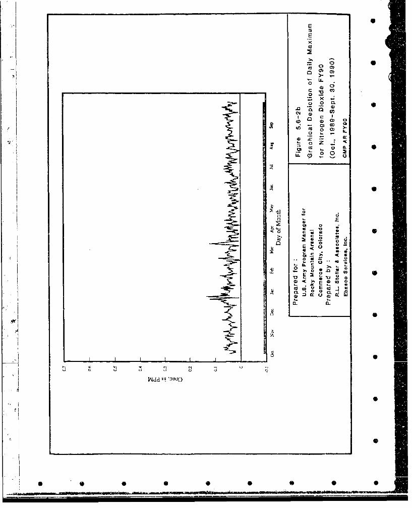
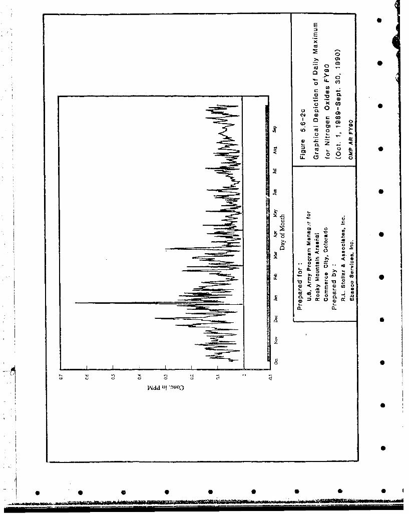
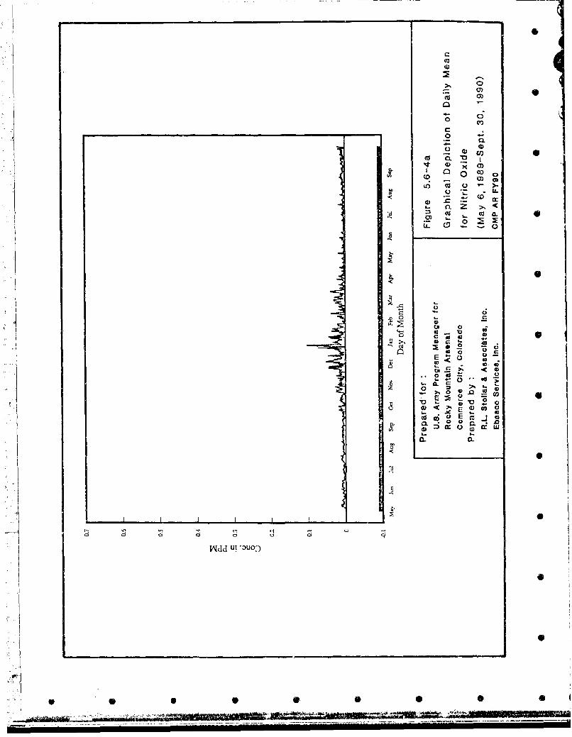
display the daily mean concentrations. Again, these graphs indicate that higher concentrations

occurred during the winter months of November, December and January.

Monthly summaries for I-hour average concentrations of NO, NO, and NO. are given in Tables

5.6-1, 5.6-2 and 5.6-.3, respectively. The National Ambient Air Quality Standard for NO, is 0.053

ppm and is an arithmetic mean. The mean for FY90, 0.016 ppm, was well below this standard.

Since seasonal and diurnal trends of NO, NO2 and NOX are interrelated, an assessment or these three

gases as a whole was made using NOX as the indicator. The diurnal cycle for these gases illustrated

a similar pattern with peak concentrations during the morning hours of 0700 MST and 0900 MST

which coincided with the Denver metropciitan area rush hour. For the remainder of the day, these

gases exhibited their lowest concentrations, although there is a slight rise again in the late evening

hoal possibly 'rom the reformation of the surface inversion. This cycle is depicted in Figure 5.6-5.

0

A comparison of the diurnal cycle for the data collection period of May through September for I ýY89

and FY90 is shown in Figure 5.6--6. The data were almost identical with a very :Iight increase of NOx

in FY90. Again, similar diurnal trends are displayed in these graphs.

0

Figure 5.6-7 depicts the overall maximum hourly concentrations and overall mean hourly

concentrations for the cumulative period of May 6, 1990, through Septenw ber 30, 1990. This graph

indicates that the individual maximium concentrations were recorded between the hours of 2000 MST

and 0400 MST and not during the morning rush hour as the diurnal pattern portrays. This may be

attributed to individual episodes in which drainage and wind flow from power plants and/or other

industrial activities resulted in peak concentrations at RMA during these hours. Figure 5.6-8

"compares the highest 24-hour nitrogen dioxide concentrations rocorded at RMA to two Colorado

.4 Department of ilealth sites for the period October 1989 through September 1990. The RMA situ 0

recorded lower values than the two Colorado l)epartment of I Alalth locations. Several case studies are':1 discussed in the next section showing the interaction of metropolitan Denver source emissions,

meteorological conditions, and ambient concentrations measured at RMA.

0

4 Individual monthly graphs and tables are presented in Appendix 1. The items contain daily maximum,

minimum and mean concentrations for eacn (lay of each imonth.

0

- 368 -

AIR -90.5.-9

.ev. 08/15/91

-%mu

i 'w

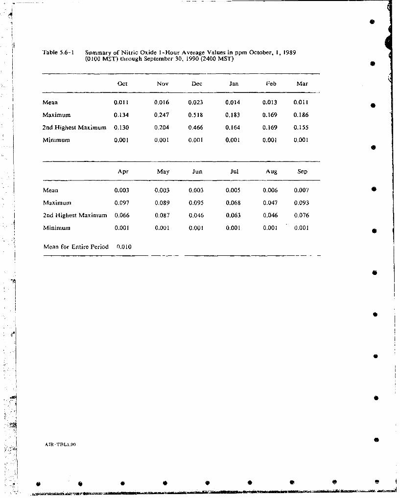
Table 5.6-1 Summary of Nitric Oxide 1-Hour Average Values in ppm October, 1, 1989(0100 MST) through September 30, 1990 (2400 MST)


Mean 0.011 0.016 0.023 0.014 0.013 0.011

Maximum 0.134 0.247 0.518 0.183 0.169 0.186


Minimum 0.001 0.001 0.001 0.001 0.001 0.001


Mean 0.003 0.003 0.003 0.005 0.006 0.007 0

Maximum 0.C97 0.089 0.095 0.068 0,047 0.093


Minimum 0.001 0.001 0.001 0.001 0.001 0.001


S

1Q

0

A0

AIR TBI.W.Q

4 "

)0

Table 5.6-2 Summary of Nitrogen Dioxide I--Hour Average Values in ppmo October, 1, 1989(0100 MST) through September 30, 1990 (2400 MST)


Mean 0.018 0.019 0.026 0.020 0.018 0.017

i Maximum 0.067 0.072 0.133 0.078 0.064 0.120


Minimum 0.001 0.001 0.001 0.001 0.001 0.001


Mean 0.012 0.010 0.010 0.012 0.015 0.015 0

Maximum 0.061 0.050 0.063 0.055 0.056 0.069


Minimum 0.001 0.001 0.001 0.001 0.001 0.001 0


Federal and Colorado Ambient Air Quality Standard for annual arithmetic mean is 0.053 ppm.

0

i..Aim

0 0 SS 41

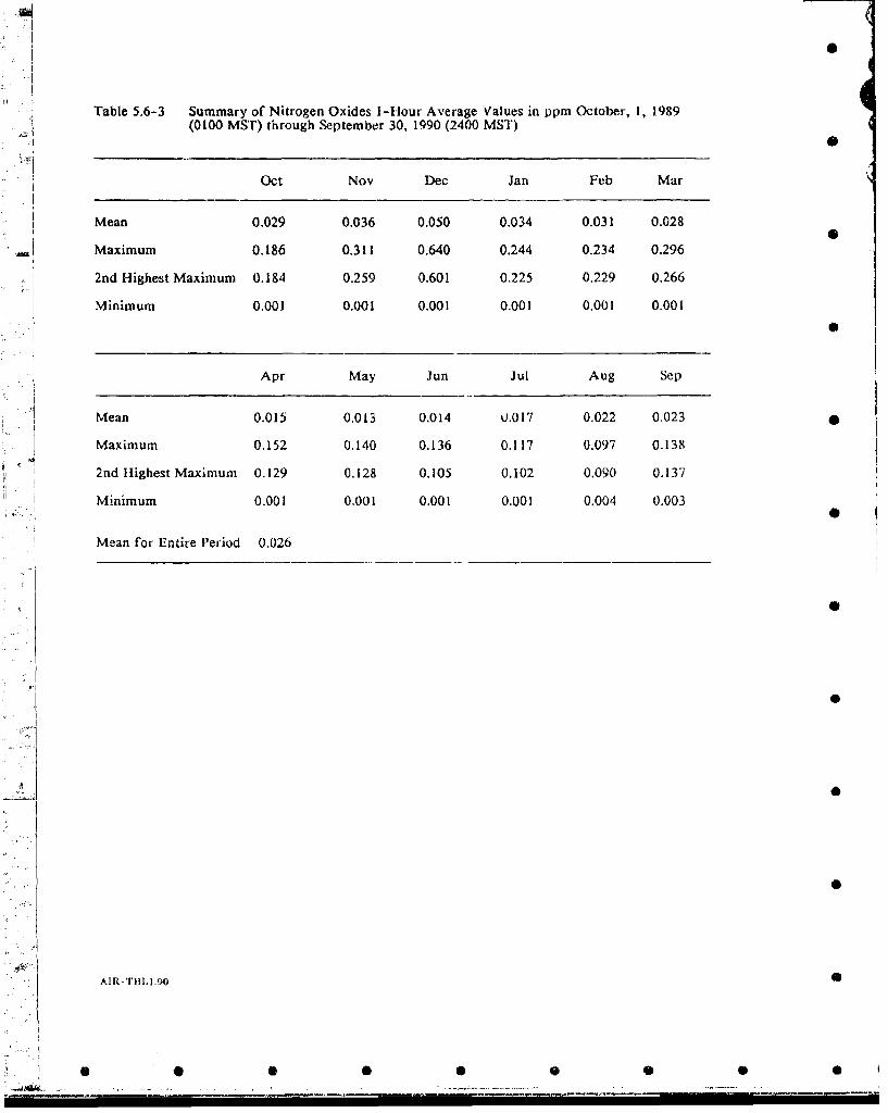
Table 5.6-3 Summary of Nitrogen Oxides I1-Hour Average Values in ppm October, i, 1989(0100 MSr) through September 30, 1990 (2400 MST)


Mean 0.029 0.036 0.050 0.034 0.031 0.028

-i Maximum 0.186 0.311 0.640 0.244 0.234 0.296


Minimum 0.001 0.001 0.001 0.001 0.001 0.001


Mean 0.015 0.013 0.014 0.017 0.022 0.023

Maximum 0.152 0.140 0.136 0.117 0.097 0.138

2nd Highest Maximum 0,129 0.128 0.105 0,102 0.090 0.137

Minimum 0.001 0.001 0.001 0.001 0.004 0.003


I0

/0

ii

AIR TI3LI.900

0 000 0 0

0)

0)

l 0 )1in 0)

0)

o 0~

oo4 32

0

0

0.0I

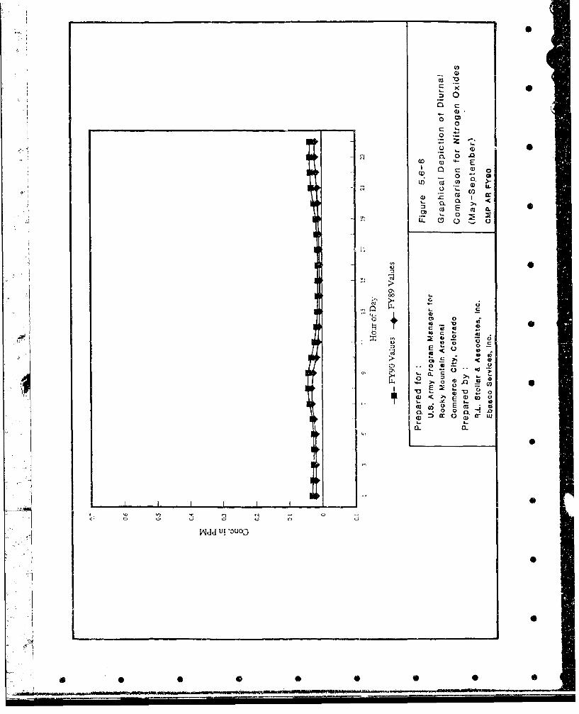
2U 0

00

0)

0

CL'

CcW 0

0 (0

0

V 0

C.:- U

co 0 '

40 la

0 40

o

ca~ E ca j0. 0 fr u 0

Wdd Ut 00) l0

fo~

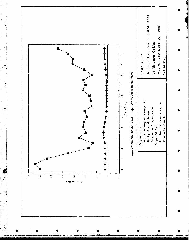
(0 00)

V)

CX 0

C 0

coo4.0

N 0) )

0

cl 0.Z).

Q CCI La

MW -6 -,o loo *2m

I

4

N02 Highest 24 Hour Concentration

0.11

0.1

0.09

0.08 -0

114 0.07 -

0006 -0

0.05

0,04

0.03 -

0.02

0 .0 1 I I I I I , I , I IOC1 NOV DEC JAN FEB MAR APR MAY JUN JUL AUG SHII

- RMA . WELBY .-, CAMP

Prepared for: Figure 5.6-8 0U.S. Army Program Manager for

Rocky Mountain Arsenal HMP and Colorado Department of

Commerce City, Colorado Health Sites 24-Hour

Prepared by Nitrogen Dioxide Values

SR.L. 8Itollar & Aaociatea, . (Oct., 1989-Sept., 1990)

Ebasco Servlces Inc. CMP AR FYO0

i S . • 0 • . 0 • •

0W0

5.7 REGIONAL EMISSION SOUVCFS IMPACTiNG RMA

Tables 5.7-1 through 5.7 3 provide 1ýstings of coiteria pollutant emissions (carbon monoxide, sulfur

dioxide, aj.J nitioger. oxides, from major rsictiopolitan Denvec industrial sources. (Table 4.1-2

previously cited in Section 4.1.4 alsu pro1-i( a more detailed listing including many smaller sources.)

Ozone (0.) is not emitted directly from ý.source as are other pollutants, but forms as a secondary

pollutant. Its precursors aee certr&1, reactive hydrocarbons and nitrogen oxides (NO.). Those sources

liste in Tables 5.7-1 4nd 5.7-3 can thercfore be considered as contributors to 03 production.

In addit~on to stalion-ýrv Sources, automobile exhaust is a principal precursor of 031 and in the winter,

V.' pioduces 86 pi, rcent of the carboi, monoxide (CO) measured in Denver and about 33 percent of theNO. (CDH, 1989). B~oth stationary and mobile emissions (primarily fw-m vehicle traffic) jointlyV ~contribute to the ambi- at air quality conditions measured at R MA. Note that F.MA gaseous emissionsshown in Tables 5.7--1 through 5.7-3 are quite smF.'ll compared to thc s.gnificant major sources in the

Denver area.

Figereý 5.7- 1 suiovws the dish it'1.tion of stationary sourco,-s suryounding RMA (sou-ce locations are

-roL~s-referewced illnbc 5.7-1, 5.7-2 adid 5.7-3). Most of, the sources are to the south and

southwest of the ~senal wheme the major veohici- activity also occurs. Monitoring , -ults from the

RMA station showeti levels of 03, C0, SC,, and NO,, that were generally belovN metropolitan Denver

mo'nitwi~ng values. Hlowever, .,,,en prevailing winds blew in ilie direction of the Arsenal with a

strone drnve-sioii and the associatcd "brown cloud" condition, external sourcos significantly impacted

the Arsenal. Thi- Nvs deinonstrated in the Air Quality Data Assessm~ent Report for FY89 (Stol~ar,

:990) and is agains; ,,in with examples from thc most recent FY90 visibility and gaseous monitoring

review o1 the air quality and meteoriological deta for RISA during FY90 indicates a number of

episods% of robable pollution migration onto the Arsenal. Case s~udics for TSP, PM-b0, metals and

VOCs Live 1beer d~'s-ussed in prior 'cctions of this report. Emphasis 'a this section is placed on

[. criteria gaseous 'ollutai;tU. As. noted, in the Tri-County area of Adams, ArapaliCe and Denver

Coutie a'' we: anuberM NRCO anid SOP pon ources and mobile source that contributed

to _~ v ý. baseline. air quality. Hy far, 1Ihe poorcst air quality day. at the Arsenal, as was the case

of' metropolitan Donvuer, were , -ciiited with the existence of intense ground-level inversions over

the area and the svbseqe.~nt .. vcl *~nint oiF the so-called "brown cloud' phenomenon. When this

la,,e,- of industrial haze, or polluition, di Aft'1 over the Arsenal, either directly or circuitously (after

-376 -

AIR? 90.5 9il'v. 08/16/91

IF..-

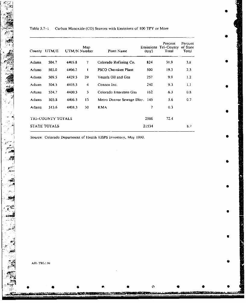
L0

Table 5.7-1 Carbon Monoxide (CO) Sources with Emissions of 100 TPY or More

Percent Percent"Map Emissions Tri-County of State

County UTM/E UTM/N Number Plant Name (tpy) Total Total

Adams 504.7 4405.8 7 Colorado Refining Co. 824 31.9 3.8 0

Adamn. 503.0 4406.2 1 PSCO Cherokee Plant 500 19.3 2.3

Adams 509.5 4429.5 29 Vessels Oil and Gas 257 9.9 1.2

Adams 504.5 4405.5 4 Conoco Inc. 24C 9.3 1.1

Adams 524.7 4400.5 3 Colorado Interstate Gas 162 6.3 0.8

Adams 503.8 4406.5 13 Metro Denver Sewage Disp. 145 5.6 0.7

Adams 513.6 4408.3 30 RMA 7 0.3

TRI-COUNTY TOTALS 2586 72.4

STATE TOTALS 21534 8.7

Source: Colorado Department of Health EISPS Inventory, May 1990. 0

A

AIR-TBLI.90

S W4 5

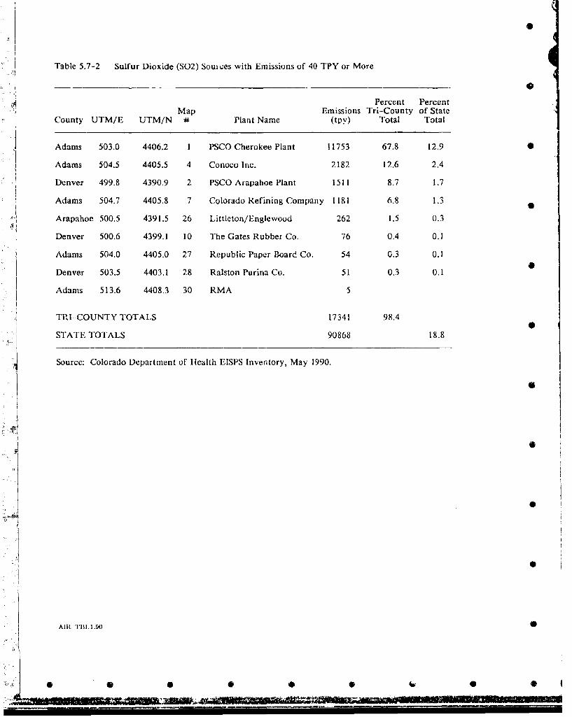
0

Table 5.7-2 Sulfur Dioxide (S02) Souices with Emissions of 40 TPY or More

Percent PercentMap Emissions Tri-County of State

County UTM/E UTM/N # Plant Name (tpy) Total Total

Adams 503.0 4406.2 I PSCO Cherokee Plant 11753 67.8 12.9

Adams 504.5 4405.5 4 Conoco Inc. 2182 12.6 2.4

Denver 499.8 4390.9 2 PSCO Arapahoe Plant 1511 8.7 1.7

Adams 504.7 4405.8 7 Colorado Refining Company 1181 6.8 1.3

Arapahoe 500.5 4391.5 26 Littleton/Engle wood 262 1.5 0.3

Denver 500.6 4399.1 10 The Gates Rubber Co. 76 0.4 0.1

Adams 504.0 4405.0 27 Republic Paper Board Co. 54 0.3 0.1

Denver 503.5 4403.1 28 Ralston Purina Co. 51 0.3 0.1

Adams 513.6 4408.3 30 RMA 5

"TI'l COUNTY TOTALS 17341 98.4

STATE TOTALS 90868 18.8

Source: Colorado Department of Health EISPS Inventory, May 1990.

0

C AIR TBIA-90

S 000 0 0

""M 11 11 1, i i

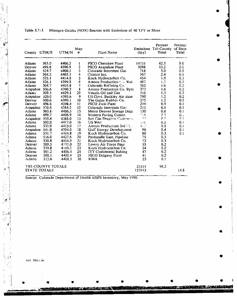
IS

Table 5.7-3 Nitrogen Oxides (NOX) Sources with Emissions of 40 TPY or More

Percent PercentMap Emissions Tri-County of State

County UTM/E UTM/N # Plant Name (tpy) Total Total

Adams 503.0 4406.2 1 PSCO Cherokee Plant 14731 62.5 9.6Denver 499.8 4390.9 2 PSCO Arapahoe Plant 3098 13.2 2.0Adams 524.7 4400.5 3 Colorado Interstate Gas 718 3.0 0.5Adams 504.5 4405.5 4 Conoco Inc. 567 2.4 0.4Adams 525.1 4414.8 5 Koch Hydrocarbon Co. 454 1.9 0.3Adams 526.1 4399.8 6 Amoco Production . Wat. 407 1.7 0.3Adams 504.7 4405.8 7 Colorado Refining Co. 382 1.6 0.2 •Arapahoe 506.6 4390.2 8 Amoco Production Co. Byrs 373 1.6 0.2Adams 509.5 4429.5 29 Vessels Oil and Gas 310 1.3 0.2Arapahoe 520.0 4395.6 9 US Govt. Buckley Air t6ase 290 1.2 0.2Denver 500.6 4399.1 10 The Gates Rubber Co. 275 1.2 0.2Denver 498.6 4398.4 11 PSCO Zuni Plant 219 0.9 0.1Arapahoe 570.6 4384.2 12 Colorado Interstate Gas 211 0.9 0.1 4Adams 503.8. 4406.5 13 Metro Denver Sewage Disp. 130 0.6 0.1Adams 499.7 4406.9 14 Western Paving Constr. 'Y' 0 0.,Arapahoe 555.4 4388.0 15 Sun C-as Dragonn Cumrr.., 0 0 IAdams 502.0 4417.0 16 US West ,' (J.J 0.1Adams 532.0 4415.0 17 Amoco Product:on 3rd "'1 1. 0.5 0.1Arapahoe 541.0 4394.0 18 Gulf Energy Developinent 96 0.4 0.1Adams 551.7 4.414.8 19 Koch Hydrocarbon Co. 80 0.3 0.1 0Adams 516.0 4427.6 20 Panhandle East. Pipeline 75 0.3Adams 530.8 4414.9 21 Koch Hydrocarbon Co. 73 0.3Denver 509.5 4397.0 22 Lowry Air Force Base 55 0.2Adams 539.8 4409.2 23 Koch Hydrocarbon Co. 54 0.2Adams 501.2 4406.4 24 ITT Continental Baking 47 0.2Denver 500.1 4400.4 25 PSCO Delgany Plant 41 0.2Adams 513.6 4408.3 30 RMA 25 0.1

TRI-COUNTY TOTALS 23551 98.2STATE TOTALS 153913 14.8

Source: Colorado Department of Health EISPS Inventory, May 1990.

A I RT , .g

S-S

AIR• TIIm~.9O

S SSS

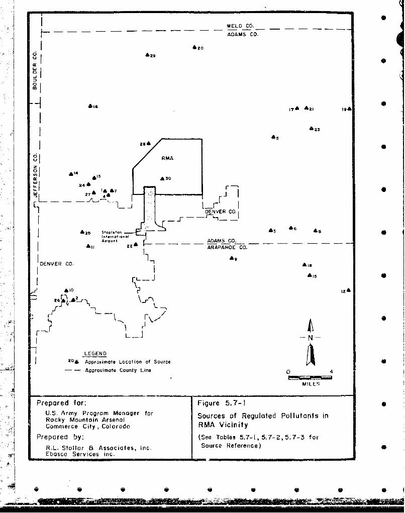
Sr. " WELD) CO.

ADAMS CO.

*1£2

2 . I &£O2-

J17r& 421 19

I£2

61 RMA

£5000

w 27A 4-F-

_ IDENVER CO.

2& 5 3top&etoi6

Infernol O0nol •'AirvorV ADAMS CO.22& - . ARAPAHOE CO.

DENVER CO.

£10 12£

D 2I r

R okyMou Aptixnrmsen LocaSure oo SR l P u t

" .! MILES

Prepared for: Figure 5.7- 1•

•,U.S. Army Program Manager for Sources of Regulated Pollutants in

"•i~t Rocky Mountain Arsenal

A . Commerce City, Colorado RMA Vicinity

2 IPrepared by: (See Tables 5.7-1, 5.7- 2, 5.7-3 f or"" , R.L. Stollar 8 Associates, Inc. Source Reference) •

"" Ebasco Services inc.

•g u m " Uminiw , • ... .- •,.••..,•••,,.:,••••

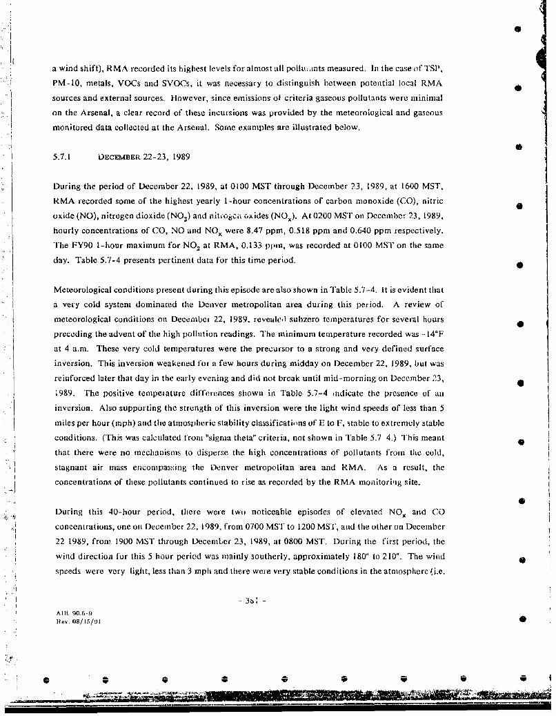
a wind shift), RMA recorded its highest levels for almost all polluants measured. In the case (f TSP,

PM-10, metals, VOCs and SVOCs, it was necessary to distinguish between potential local RMA

sources and external sources. However, since emissions of criteria gaseous pollutants were minimal

on the Arsenal, a clear record of these incursions was provided by the meteorological and gaseous

monitored data collected at the Arsenal. Some examples are illustrated below.

0

5.7.1 DECEMBER 22-23, 1989

During the period of December 22, 1989, at 0100 MST through December 23, 1989, at 1600 MST,

RMA recorded some of the highest yearly 1-hour concentrations of carbon monoxide (CO), nitric

oxide (NO), nitrogen dioxide (NO.) and njitcogcii oxides (NO.). At 0200 MST on December 23, 1989,

hourly concentrations of CO, NO and NO, were 8.47 ppm, 0.518 ppm and 0.640 ppm respectively.

The FY90 I-hour maximum for NO 2 at RMA, 0.133 ppim, was recorded at 0100 MST on the same

day. Table 5.7-4 presents pertinent data for this time period.

Meteorological conditions present during this episode are also shown in Table 5.7-4. It is evident that

a very cold system dominated the Denver metropolitan area during this period. A review of

meteorological conditions on December 22, 1989. revealcel subzero temperatures for several hours

preceding the advent of the high pollution readings. The minimum temperature recorded was --140F

at 4 a.m. These very cold temperatures were the precursor to a strong and very defined surface

inversion. This inversion weakened for a few hours during midday on December 22, 1989, but was

reinforced later that day in the early evening and did not break until mid-morning on December 23,

1989. The positive temperature differences shown in Table 5.7-4 indicate the presence of an

inversion. Also supporting the strength of this inversion were the light wind speeds of less than 5

miles per hour (mph) and the atmospheric stability classificati-ms of E to F, stable to extremely stable

conditions. (This was calculated From "sigma theta" criteria, not shown in Table 5.7-4.) This meant

that there were no mechanisms to disperse the high concentrations of pollutants from the cold,

stagnant air mass encompassing the Denver metropolitan area and RMA. As a result, the

concentrations of these pollutants continued to rise as recorded by the RMA monitoring site.

0

During this 40-hour period, there were two noticeable episodes of elevated NOx and CO

concentrations, one on December 22, 1989, from 0700 MST to 1200 MST, and the other on December

22 1989, from 1900 MST through December 23, 1989, at 0800 MST. During the first period, the

wind direction for this 5 hour period was mainly southerly, approximately 180* to 210'. The wind 0

speeds were very light, less than 3 mph and there were very stable conditions in the atmosphere (i.e.

I ~- 3a1 -

All? 90. 9Rev. 08/ 1 /91 0

.- !2 . ... .

cz P onýt w m nCD . It In * 1

N C ý ' 't N 1 l 60I-O 0' 0: 0ý '0 -*' C N p!60r~ It - 0-N 1' (

Q w 0 P. 0, 't N .

N IC .M ' CI 11m C"m24M"

1919a

W% m0% nI . Sr - ne

000 0 0 " S 0-nN 0 - 0 ' O 0t

0'00 0000 000 000o 0000 0000 000o

o o'mo fn cm -C"

4)m mC >QCa v ýC3a a Q C,0C. 3< D- DC

VL r l A -

a D) 0 0 0 0 00CC>ý0 C,0 0 0 ODC )0000a00 a00000000C, L*Cý ý'U uC

to

0$

-1 en 0 ('L0L1000 ~ ~ C 0 'oV . 0 ~ N ~ '

CdI-C.0C ~ C OF C J C

o ~ ~ ~ ~ ~ ~ - 't'' . ' 0 '-I(~f

If' . . . .

,. Q 0 ýC - M' n C NJ' - rn tlK

vp ` c3 c' cy~fN NI.J NN .o ~~~~~~ N(N rN'N N II NN9l~.I.J N 30`c

~~14HC

fb 0

4u r4F nS-

00

0d q

-i >

Cl 6u

coc. cooc

14)

0j cm 0ve l

2c I0

little or no mixing). Figures 5.7-2, 5.7-3 and 5.7-4 depict peak concentrations at the RMA

monitoring site for this event for carbon monoxide, sulfur dioxide and oxides of nitrogen,

respectively, Possible causes for the increase in concentrations during this episode, in addition to the

wind flow from metropolitan Denver in the direction of the Arsenal, includ.': 1) the morning rush

hour from the Denver metropolitan area; 2) emissions from the nearby large source•; 4,_,.it as Public

Service Company - Cherokee Plant (see map designator #1 on Figure 5.7-1); 3) air traffic from •

Stapleton Airport; 4) a composite of the above and other metropolitan industrial activity, trapped

under a very intense inversion and drifting toward RMA.

During the socond period, the wind direction returned to a southwesterly component of approximately 0

225* after it changed to a northerly component. Again, the wind speeds were very light at less than

5 mph. Atmospheric conditions for this 9-hour period of extremely high concentrations were

primarily stable to very stable (E to F stability class). These conditions were largely responsible for

the poor air quality that was recorded during this period. Possible causes were the same as those

stated for the first period, it is also possible that pollutants recorded earlier that migrated northward

may have been "rechanneled" back into the Denver metropolitan area due to the changing winds, thus

adding to iorm already accumulating "pool' of pollutants. This is not an uncommon situation because

of the bi-miodal upslope and downslope (drainage) pattern across the metropolitan area.

5.7.2 MAY 21, 1990

During the period from n100 MST throu[;h 1200 MST on May ^'1, 1990, the RMA recorded the

higl.est yearly 1-hour concentrations of sulfur dioxide (SO 2). At 0800 MST of this day, the hourly

concentration of SO 2 was 0.05 ppm. Thi'i day was unique because the highest I-hour concentration

of SO, was recorded, but the other relevant air quality parameters of carbon monoxide including

nitric oxide, nitrogen dioxide and nitrog;en oxides were typical of the mon" g rush hour pattern,

showing some elevations but no obvious peak concentrations.

The air quality and meteorological conditions that were present during this episode are presented in

Table 5.7-5 and are also illustrated in Figures 5.7-5, 5.7-6 and 5.7-7. From these data, it is noted that

the concentrations of all air quality parameters were near normal from 0100 MST to 0600 MST. There

were slight increases La NO, NO2 and NO., but again hardly a notable rise in the concentration.

f • During these early hours of the morning, winds were primnirily from the south to southwest; however,

ý.J wind speeds were at first moderate (8 to 11 mph) and atmospheric stability was neutral. About 0400

"MST, the surface inversion began to gain strength (stability categories E and F) and wind speeds

384

. /

*

December 22 - December 23,1989Carbon Monoxide Concerdralionts

3mph

8-

7 0

4 - WM NNW 0y8 7~d @ 7ph

Mkid SE5 mnph

Qr-n-- I Il I I I I rrriT1 3 5 7 9 11 13 15 17 19 21 ' 1 3 5 7 9'11 13 15

I our ofD.,Goo

S

0

i~i..

Prepared for: Fiue5720U.S. Army Program Manager for Fgr .-Rocky Mourntain Arsenal Graphical Depiction ofCommerce City, Colorado Carbon Mono xide for

Prepared by: December 22-23, 1989R.L. StoMllr & Associates,. Inc,

Ebasco Services Inc. CMP AR FY90

09 w.sw S•

December 22 - December 23, 1989Sulfur Dioxide Concentrations _0.025-

3 rnpt

0.02-0

E 0 .0 1 5 " W W id N NW, @

5 nvh 7 mph 1

0 .01 '2.8 m• i

V" S1 @0.005 .

1 5' 79 11 13 15 17 19 213 1 3 5 7 9 11 15Hour of Day

- S02

Prepared for: Figure 5.7-3U.S. Army Program Manager for

Rocky Mountain Arsenal Graphical Depiction ofCommerce City. Colorado Sulfur Dioxide for

Prepared by : December 22-23, 1989R.L. Gtollar & Associates. Inc.

Ebasco Gervices Ina. CMP AR FY90

0! 0 0 0 0 • 0

=0

41 0

December 22- December 23, 1989Oxides of Nitrogen Concentrations

0.7 w,,ws•

0.6-

0.5-

E 0.4-

8 0.3- 7.1 ,,ph

0.2 wnsc@

5. ~rnph

-l 0S1 3 5 7 9 11 13 15 17 1'9 21 23 1 3 5 7 9 11 13 15

Hour of Day

- NO -- N02 - NOx

Prepard forFigure 5.7-4U.S. Army Program Manager for

Rocky Mountain Arsenal Graphical Depiction of*Commerce City. Colorado Nitrogen Oxides for

Prepared by December 22-23, 1989R.L. Stoller & Associates, Inc.

*Ebmaco Services Inc. CMP AR IFYvrj

- 2

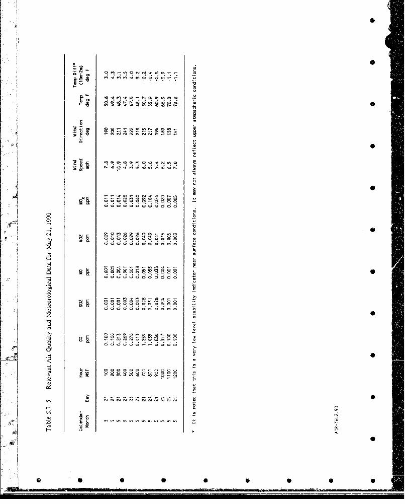
41

c) rj' tc

C>C

-o4) O -1 . r l

0 0 0 0 0 0 0 0 Al

zO.

cd >~.

o~C Oo D O .,N O

x 0 ol In r- s :

0n0In0. .- - 0--00I0I

Cd 2c

0

May 21,1990Carbon Monoxide Concentration1.4 / sw

1.2-

1S/ 0

:0.8-

0.6

Wr-d WSW- 00.4- 1 wV Wn SE

7mih -

0.2' - - -1

1 2 3 4 5 6 7 0 9 10 11 12Flour of Day

-÷- CO 0

00

Prepared for: Figure 57-5

U.G. Army Program Manager for

Rocky Mountain Arsenal Graphic AI Depiction ofCommerce City. Colorado Carbon Monoxide for

Prepared by May 21, 1990R.L. Stollar & Associates, Inc. 0Ebasco Swrvlcos Inc. CMP AR FY9O

• 0 0 0 0 0 0 0

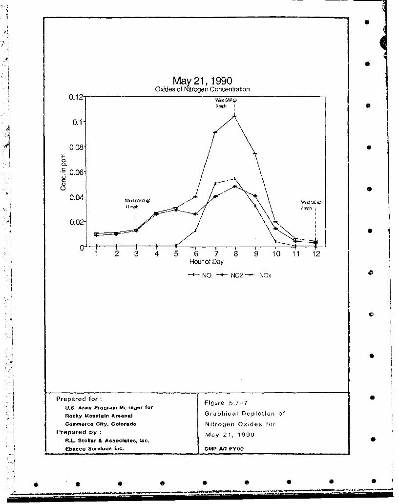
Oxides of Nitrogen Concentration0.12 -C Sw sw

6 lph I

0.11"

008 0E

,, 0.06

0.0--•0.026-

0* I

1 2 3 4 5 6 7 8 9 10 11 12Hour of Day

' NO N02 -- NOx

Prepared for:• " repaed fr :Figure 5.7-7

U.S. Army Program Me iager forRocky Mountain Areenal Graphical Depiction of

Commerce City, Colorado Nitrogen Oybdes forPrepared by : May 21, 1990

RA. Stollar & Asaoclates, Inc. -

Ebacco Servicea Inc. CMP AR FY9O

0. .0. .....

decreased (4 to 5 mph). Pollutant levels increased during the next sev.;ral hours reaching peak

concertt-ations at 0800 MST. Shortly thereafter, th, inversion began to dissipate and all criteria

pollutant levels decreased to normal baseline values, very likely that the source of the higher SO 2

concentrations at 0800 MST was the Public Service Cot oany - Cherokee ?lant. The win(' direction

for the 3 previous hours, and for the hour of highest concentrations, was from the southwest,

approximately 220'. This -orresponds to the location where the plant would be directly upwind from

the Arsenal.

It is of interest that the peak CO concentration at RMA, 1.26 ppm, was attained at 0700 MST while

the peak SO, concentration occurred at 0800 MST. This might be explained by the vertical stability

and wind profiles. Carbon monoxide is emitted from low level sources, resulting primarily from

metropolitan Denver automobile traffic. At 0800 MST, the ground level stability (from "sigma theta"

calkulations) was already slightly unstable (category C) and CO levels began to decrease rapidly,

returning to its lowest levels before noon when the atmosphere became highly unstable (category A).

The winds also shifted, blowing toward the northeast away from the Arsenal. Sulfur dioxide, on the

other hand, is emitted from higher level sources ruch as the tail stacks at the PSC Plant. It is unlikely

that surface heating reached the height of the SO, plume until shortly after 0800 MST when

concentrations began to decrease at the RMA site similar to the CO pattern.

The peak SO, concentration at RMA was considerably below the short-term Colorado Ambient Air

Quality Standard (0.50 ppm for 3 hours). However. this example demonstrates how closely ambient

concentrations from a pollutant emission source were determined by meteorological factors, and, in

pamiicular, wind flow and atmospheric stability. Since RMA is not a major source of criteria

pollutants, all peak concentrations measured at the Arsenal were a reflection of the dispersion of

emissions from upwind mobile and stationary sources (as shown in Figure 5.7-1). The CMP has

documented numerous case studies ranging from typical morning surface inversions with modest

impacts at RMA to intense winter surface inversion episodes and associated "brown cloud" conditions,

where impacts on the Arse-nal have been sever.0 . These impacts, controlled by meteorological

conditions, included not only gaseous pollutants but other components of industrial pollution such as

TSP, PM-10 and metals discussed elsewhere in this report. Stiil another consequence is the -ffect on

am.bient. visibility which 's discussed in the next section. As will be shown, there were strong

similarities and interrelationships between all of thesc effects.

- 392

R'..08/15/91 •

0.... 0ii - n.... i.. .i. . .. i - ' - - ....0 0 ... .0 - - 0.. 4 ... .i......

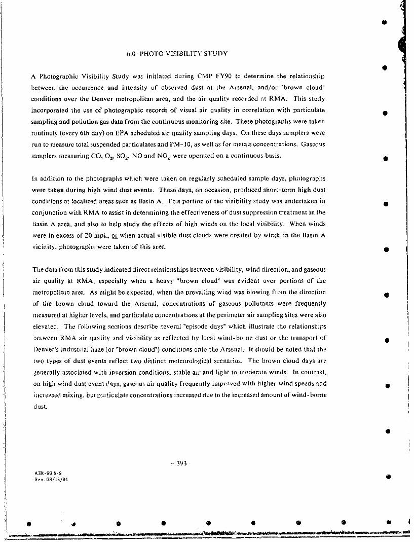
S

6.0 PHOTO VISIILITY STUDY

A Photographic Visibility Study was initiated during CMP FY90 to determine the relationship

between the occurrence and intensity of observed dust at the Arsenal, and/or "brown cloud"

conditions over the Denver metropolitan area, and the air quality recorded mt RMA. This study

incorporated the use of photographic records of visual air quality in correlation with particulate 0

sampling and pollution gas data from the continuous monitoring site. These photographs were taken

routinely (every 6th day) on EPA scheduled air quality sampling days. On these days samplers were

run to measure total suspended particulates and PM-10, as well as for metals concentrations. Gaseous

samplers measuring CO, 0, SO 2, NO and NO. were operated on a continuous basis. •

In addition to the photographs which were taken on regularly scheduled sample days, photographs

were taken during high wind dust events. These days, on occasion, produced short-term high dust

conditions at localized areas such as Basin A. This portion of the visibility study was undertaken in •

conjunction with RMA to assist in determining the effectiveness of dust suppression treatment in the

Basin A area, and also to help study the effects of high winds on the local visibility. When winds

were in excess of 20 mpl,, or when actual visible dust clouds were created by winds in the Basin A

vicinity, photographs were taken of this area. •

The data from this study indicated direct relationships between visibility, wind direction, and gaseous

air quality at RMA, especially when a heavy "brown cloud" was evident over portions of the

metropolitan area. As might be expected, when the prevailing wind was blowing from the direction •

of the brown cloud toward the Arsenal, concentrations uf gaseous pollutants were frequently

measured at higher levels, and particulate concentiations at the perimeter air sampling sites were also

elevated. The following sections describe zeveral "episode days" which illustrate the relationships

between RMA air quality and visibility as reflected by local wind-borne dust or the transport of 0

Denver's industrial haze (or "brown cloud") conditions onto the Arsenal. It should be noted that the

two types of dust events reflect two distinct meteorological scenarios. The brown cloud days are

generally associated with inversion conditions, stable air and light to moderate winds. In contrast,

on high w'nd dust event days, gaseous air quality frequently improved with higher wind speeds and

increamed mixing, but p'articuiate concentrations increased due to the increased amount of wind-borne

dust.

- 393 -

AIR-90.5-9Rev. 08/15/91

0 000

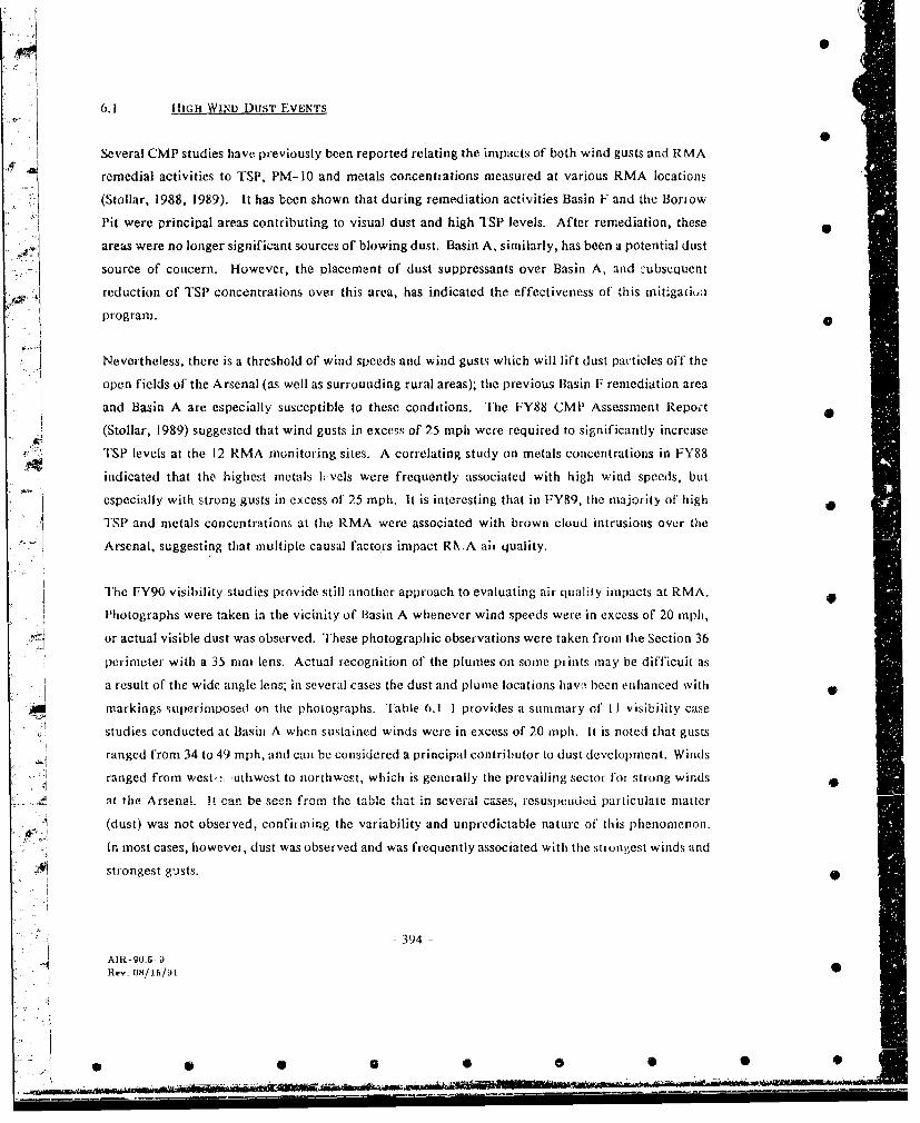
6.1 HIGH WIND DUST EVENTS

Several CMP studies have previously been reported relating the impacts of both wind gusts and RMA

remedial activities to TSP, PM- 1 and metals concentrations measured at various RMA locations

(Stollar, 1988, 1989). It has been shown that during remediation activities Basin F and the Bornow

Pit were principal areas contributing to visual dust and high TSP levels. After remediation, these

areas were no longer significant sources of blowing dust. Basin A, similarly, has been a potential dust

source of concern. However, the Dlacement of dust suppressants over Basin A, and -ubsequent

reduction of TSP concentrations over this area, has indicated the effectiveness of this mitigatia

program.

Nevertheless, there is a threshold of wind speeds and wind gusti which will lift dust particles off the

open fields of the Arsenal (as well as surrounding rural areas); the previous Basin F remediation area

and Basin A are especially susceptible to these conditions. The FY88 CMP Assessment Report

(Stollar, 1989) suggested that wind gusts in excess of 25 mph were required to significantly increase

TSP levels at the 12 RMA monitoring sites. A correlating study on metals concentrations in FY88

indicated that the highest metals lvels were frequently associated with high wind speeds, but

especially with strong gusts in excess of 25 mph. It is interesting that in FY89, the majority of high

TSP and metals concentrations at the RMA were associated with brown cloud intrusions over the

Arsenal, suggesting that multiple causal factors impact RN.A air quality.

The FY90 visibility studies provide still another approach to evaluating air quality impacts at RMA.

Photographs were taken in the vicinity of Basin A whenever wind speeds were in excess of 20 mph,

or actual visible dust was observed. These photographic observations were taken from the Section 36

perimeter with a 35 mm lens. Actual recognition of the plumes on some prints may be difficult asa result of the wide angle lens; in several cases the dust and plume locations hawv been enhanced with

markings superimposed on the photographs. Table 6.1 I provides a summary of I I visibility casestudies conducted at Basin A when sustained winds were in excess of 20 mph. It is noted that gusts

"ranged from 34 to 49 mph, and can be considered a principal contributor to dust development. Winds

ranged from west-!, uthwest to northwest, which is generally the prevailing sector for strong winds

at the Arsenal. It can be seen from the table that in scveral cases, iesuspwmdcd particulate matter

(dust) was not observed, confirming the variability and unpredictable nature of this phenomenon.

In most cases, however, dust was observed and was frequently associated with the stroniest winds and

strongest guists.

394 -

AI -90.5 9.Rev. 08/165/9

2 0

ing W-0, Q"~~

Table 6.1-1 Summary of High Dust Events During FY90

Wind Speed Peak GustDate Time (mph) (mph) Direction Observation

!1-06-89 1215 20-23 34 NW No dust observed

"11-06-89 1230 20-23 34 NW Some low dust

12-05-89 1430 20-26 37 NW Widespread dust, entire area

01-08-90 1110 22-27 44 WSW General low level dust, entirearea

01-10-*90 1340 22-24 44 NW Light, low level dust cloud overcenter of Basin A

04-28-90 1025 19-27 41 WNW Light, low level dust cloud overBasin A

0

05-15-90 1245 11-24 46 WNW Widespread dust over Basin A;very high TSP levels (250 ,tg/ni)just south of Basin A

"05-18-90 1430 22-30 47 NW V lespread dust over Basin A

06.-21-90 1420 15-28 41 NE Light, low level dust cloud overBasin A

07-23-90 1525 14-15 39 NW Light, low level dust cloud overBasin A

09-10-90 1440 10-24 49 N Low level dust over Basin A, butno distinct dust cloud

AIR-M-~1.90

0 S S 0

0 0-ll-0

0

A typical strong dust event day was May 15, 1990 (see Figure 6.1-1). This was a very gusty day with

a large amount of visible wind-borne dust. An observer at the Arsenal noted that small gravel was

airborne along with the sand and dust. The maximum gust measured by the meteorological tower

nearest to the site of the photograph was 46 mph. Winds were variable throughout much of the day,

but were primarily from the southwest to northwest during the midday period. The photographs

presented in Figure 6.1-1 show extremely reduced visibility in the Basin A vicinity. A group of large

storage tanks about 200 yards from the photographer were r~early invisible behiad airborne dust.

May 15, 1990, was not a routinely scheduled TSP sampling day. However, because of the forecast

for high winds, high event monitoring was conducted on this date at a number of RMA monitoring

sites. Table 6.1-2 shows the results of TSP monitoring for the period from 0800 MST on May 15

through 0800 MST on May 16, 1990.

Table 6.1-2 TSP Monitoring Results for May 15, 1990

Monitoring Site Concentration (ug/m 3 )

AQI 3.-Y.6AQ3 51.5AQ4 43.9AQ5 25.4AQ6 55.1AQ8 33.8Mobile East 36.7Mobile West 250.5

The greatest impact was experic i-d at Mobile West (Sampler No. M 113), which was located in the

extreme northeast corner of Section 2, south of' the Basin A Neck construction area. Other sites

appeared to be above their normal TSP levels, in particular AQ6 which was also downwind from Basin

A during much of the monitoring period. Hlowever, it is most interesting that except for Mobile West,

impacts were not excessive; the event (shown in the photographs) was transitory (dust was lifted

1.)!iarily during the peak gust period) and somewhat localized. The annual FY90 TSP results

substantiate the effectiveness of the mitigation actions taken at Basin A and Basin F. On the other

hand, the high levels at Mobile West confirnm the difficulty in controlling dust under very high gust

conditions during active construction activities.

- 396

AIR- 90.5-9Rev. 08/16/91

0 0 S 0 0 S 0

Figure 6.1-I Dust Event Case Study: May 15,1990

PHOTO 1: Time of Day: 1250 MST Direction of Photo: West-northwest

Note: High, heavy clouds of wind-borne dust obscure most details in the photo.The storage tanks to the left are about 200 yards from the photographer.

PHOTO 2: Time of Day: 1250 MST Direction of Photo: Northwest

Note: There is a very visible white dust cloud in the center of the photograph,in Basin A. Windblown dust closer to the photographer reduces clear visibi]ity inthe foreground.

Air quality criteria pollutants were measured at moderate concentrations prior to the advent of highwind gusts at 0800 MST; the levels of CO, NO. and SO 2 reflected the typical morning increase of thepollutants associated with the morning rush hour traffic activity south and west of the Arsenal. Thelevels of all criteria pollutants (except ozone) dropped dramatically when the wind speed increased.

This is shown in Table 6.1-3 which provides a continuous record of criteria pollutants andS4 rmeteorological data taken at the RMA monitoring sites. An abrupt change is noted at 0800 and 0900MST coincident with the increased wind speed and wind gust conditio is. Pollutant patterns associatedwith this change are also illustrated in Figure 6. 1-2. It is of interest that although criteria pollutantlevels remained iow, the poorest visibility conditions (reflected by the photographs in Figure 6.1-1)occurred near 1300 MST, when peak gusts reached 46 mph.

A 6.2 BiowN_ CLOUD EVENTS

Photographs were tal,'n from the M4/AQ site locatio,, on each air sampling day. These photographsrecorded visual condih ons from the southwest to thc northwest between RMA and the mountainslocated to the wct of the Denver metropolitan area. On days of inclement weather which severelyli!nited visibility, no photographs were taken. In addition to the photographic record, informationsuch as weather conditions, ground conditions and general visibility were recorded on a data sheet.These data and the photographic evidence were then compared with gaseous data and particulate

A .... sampling results from that day. It should be stressed that the purpose of these evaluations was not toprovide a definitive brown cloud study; the purpose rather, was to identify the impacts ofmetropolitan Denver industrial pollution on RMA air quality (and visibility) as measured under theCMP, and to distinguish between local RMA emissions and impacts, and external off-Arsenalemissions and impacts that comprise the RMA air quality baseline.

Once the photographs were returned from processing, further evaluation of conditions was made. Asupplemental data shuet recoided the visibility of landmarks of known distances, and otherobservations made in evaluating the photographs. Both upper level visibility, which included MountEvans, and lower level visibility were judged. During the sumnii.'r months, visibility at both levelswas usually good, but during the winter, visibility was frequentrv reduced, especially at the lower 3

"TA levels. The presence of a surface inversion and light winds usually created this lower level foorvisibility scenario. These atmospheric conditions retarded the mixing between the colder lower levelair and the warmer upper level air, and pollutants became trapped and concentrated in the lower airmass. -

¾ - 398-

AIR 90.5-9

H ey 0,8/16 /9 1

TEN - S 1

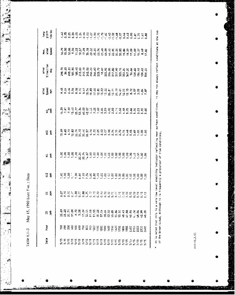
In 4'f

C;, 't 0O

Cg C, nICIý C'00In * I-

INNN "

49 C!O . . . . .

ItN. 1 0 C 1- -

Mi CU'0 cj r 4 n' 6 nu

U'..- Q rN- 0u gr rn a

N2 IN 0

N V0

9 O C! r "I .ooooooo o 0oC. nooo

OC 09 C C) n 0 0 0 l 0 0 0 0

O'40- . .0 . .2 .n . ... .4 0 .f .5 , . ' . 4 . . . . aIn3 'CNN-ON-cf, Ca In t4CD.40O Cd 'C . )0

(nt fn go 00Fnw

oZ C 000 0 03 0n 0ý In 0 0 0 0 0ý 0 0:

'T ~ ~ ~ ~ * -. wA N, CD C n-tIN n('4

-0 - --

Dust Event: May 15, 1990S02 and NOx Concentrations

70-

wind S-SW

60- 8mph

50-

40-

( 0

W•nd N E 13mphn mph@ 46 mph gust

9m-,h (Timo of photo)20 16 mph gust Wind W @

2 20mph Wind NE @

I30 mph gust 8 mph10 17 mph gust

10-II

3 7 9 11 13 15 17 19 21 23Hour of Day

- S02 -- NOx

Prepared for : Figure 6.1-2 •

U-S. Army Program Manager for

Rocky Uountain Arsenal Dust Event May 15, 1990

Commerce City. Colorado (SO 2 and NOx)

Prt-pared by

RA. Stollar & Associates. Inc.

Ebasco &ervice-.. Inc. CMP AR IFYO0

-. Al 09990 0

Upper level visibility was judged by the clarity of the high mountains visible from the RMA. Lower

level visibility was judged by the clarity of closer landmarks such as the foothillM and tie buildings

of downtown Denver, which were obscured when a brown cloud was suppressed by a surface

inversion. Visibility was classified as excellent, good, fair or poor depending upon the clear visibility

of certain landmarks.

The judging criteria were as follows:

Excellent Visibility - Mount Evans (52 miles) was clear and sharp, as were all

foreground landmarks.

Good Visibility - The foothills and Hogback (21 miles) were clear and sharp, even at the

very bottom. Mountains may or may not be clearly visible.

Fair Visibility - The foothills and Ilogback were indistinct, but the D3enver skyline ( 0.5

miles) was clearly visible.

Poor Visibility - The Denver skyline was not distinct, or not visible.

Thirty-eight percent of the cases were in the poor visibility category. It should be noted that the

scheduled photographs were taken during the morning periods when rush hour traffic was heaviest,

and the gaseous pollutants measured at the RMA continuous monitoring site were generally at their

highest levels; when inversion conditions persisted, visibility was frequently at its poorest levels for

the entire day as well. The photographic record kept during FY90 has proven useful in evaluating

' above average gaseous pollution days at RMA.

When the brown cloud was unmistakably evident, and the wind blew from metropolitan Denver across

RMA, gaseous pollutant concentrations were consistently higher than normal. As might be expected,

on days when a surface inversion existed, but the brown cloud drifted away from the Arsenal, normal

or better than average air quality readings were recorded at the Arsenal. It is interesting that on

several days when the brown cloud was transported to the north or northwest of Denver under a

southerly wind flow, and winds then shifted to a steady westerly or northwesterly component, air

quality criteria pollutant levels abruptly increased at the Arsenal moritoring site. Data strongly

suggest that the air quality of the RMA is directly influenced by the presence and position of' the

-401-AIR-90.b -9Vey. 08/15/a1

brown cloud. Several examples illustrating brown cloud impacts under various meteorological

scenarios are provided below.

* October 25-128

October 25, 1989, was a day with particularly poor visual air quality. Though the upper level °

visibility was good and distant mountains could be seen clearly from RMA, the lower level visibility

was poor, The foothills, particularly the lower portion, were obscured by an obvious brown haze.

The brown cloud, as evidenced by the photographs in Figure 6.2-1, was most dense toward the north,

but stretched all along the front range; Photo 1 is directed to the southwest and Photo 2 is directed

to the northwest from the Arsenal monitoring site.

The wind varied f-om south-southwest in the early morning hours to westerly around midday, then

northwest from early afternoon to late evening when it turned again to a southerly wind. The winds,

therefore, pushed the brown cloud toward the north and northeast during the early hours of the day,

then to the east (toward the Arsenal) at midday. Tabla 6.2-1 provides a continuous record of criteria

pollutants and meteorological data collected at RMA on October 25, 1989. The result of the wind

shifts was that the brown cloud remained upwind of the RMA continuous air monitoring site until

late morning when the westerly component of the wind resulted in increased criteria pollutant levels

recorded at the Arsenal monitoring site. Figure 6.2-2 illustrates the migration of the brown cloud

with wind shifts during the day.

0

The recorded values for all gaseous parameters except ozone were noticeably higher than the October

monthly averages and the yearly averages. Since ozone production is a photochemical process and the

day was uniformly overcast, ozone production would be expected to be lower than normal. Figures

6.2-3 and 6.2-4 present the daily summary of gaseous (SO 2 , NO., and CO) data, as well as pertinent

meteorologicatl data for October 25, 1989. These figures illustrate trends in concentrations of

representative gaseous pollutants throughout the day. In general, there appears to be a slight lag

between wind direction shifts a-id gaseous pollutant concentrations.

As a regular air sampling day, October 25, 1989, also registered considerably higher than normal TSP

and PM-10 particulate concentrations at all sites, as well as elevated metals levels at some sampling

sites. The highest particulate concentrations collected during this day were at the perimeter air

sampling stations at the west (AQI), and northwest (AQ2) boundaries of RMA. AQI measured 133

&pg/m3 and AQ2 measured 161 pg/M 3 , exceeding the Colorado 24-hour AAQS. The October 25 data

- 402 -

AIR 90.5 9Reyv. 08/15/91

* 0 0 06 0 0

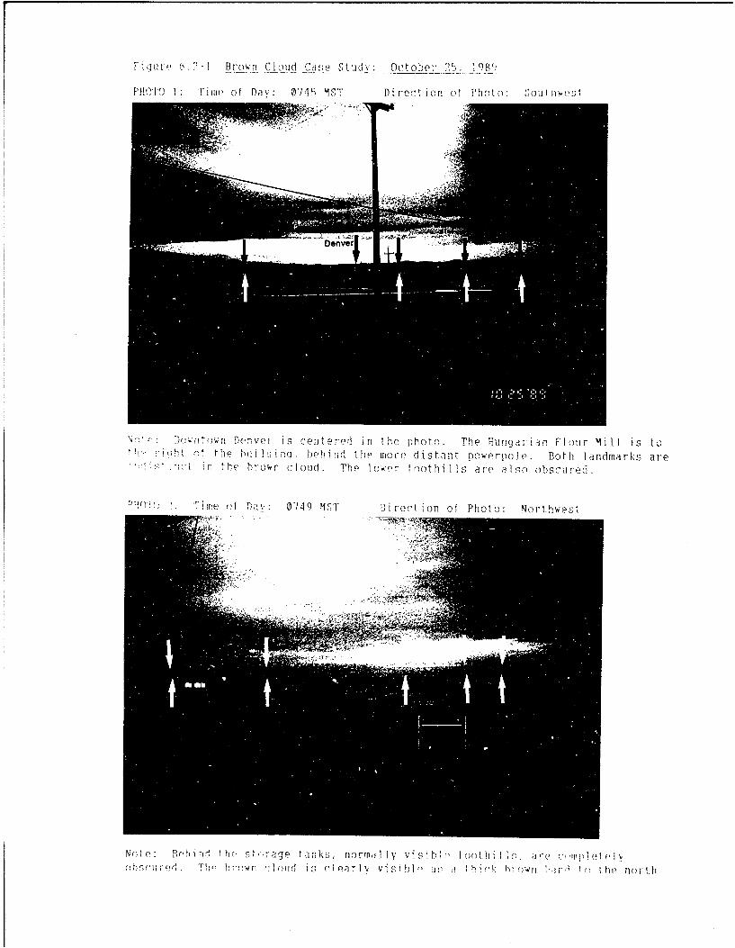
Tiltu o .- I -B C I Could- C"-s( qte lid v Oc t-olbeiv 2- 1 980

PiV : Fiiiie of Dav : 07 4 1 MST D i rect io OT at Photo: ;OUt ItWPSt

DrrtwriDenvei is cent erect in the photco. The Hungar~ian Hlour Mill is to:;h 2 thi~ ht i Himflu heih i'il the, mincr distant powerpol e Both landmarks are

i i in the brown cloud. T h. loIwr foothi 1 I s are also obs-uredl.

Tt tf2 f p Day v 0-49 IIS1' D)i ce( t i on of Photo: Nort-hwes,

No t e: Bi r!l s, r:rage t; us normal ly WI isH ; toot hi 1s . e ar 1;~i~a[ohoci,.ad Tb ht-mWrT I 011d i scI e arlI v si 1) hi h: n oh braw H 1 . i t

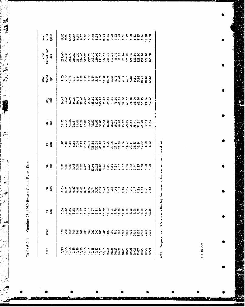
O0 PQ00000 0000 0n* o.

~~~~ 0, N~ C 0i n - 0 @ 3CCS 0 0t 'n

C4 0-11- C4O M. C~ C4 4 mm Fn.-- om

ONJO .00 !3 0, %0W% P oM ' W N m

.0 Nfl 000 M u t Cý C) C- N iC.) 1- O a-i oo - . . .

14.0

0, w ' 4 p P 0 (1W)

O O O Or- w m - - - --m- - -00 *m' 0C4 :2 'n (Mej 2

0lC ;0wQ.

C)r mr ' S 0 . . @ S N C 3 .01 O .-A .Pt.t ,C

U0 4)ý C C ol0C Cnnfiiiiih~nnnnnnD .0inCD0 C> C.0i

IR -o C?2,2Fl-G

I-i 0nir m( Ii( ý

cl 12

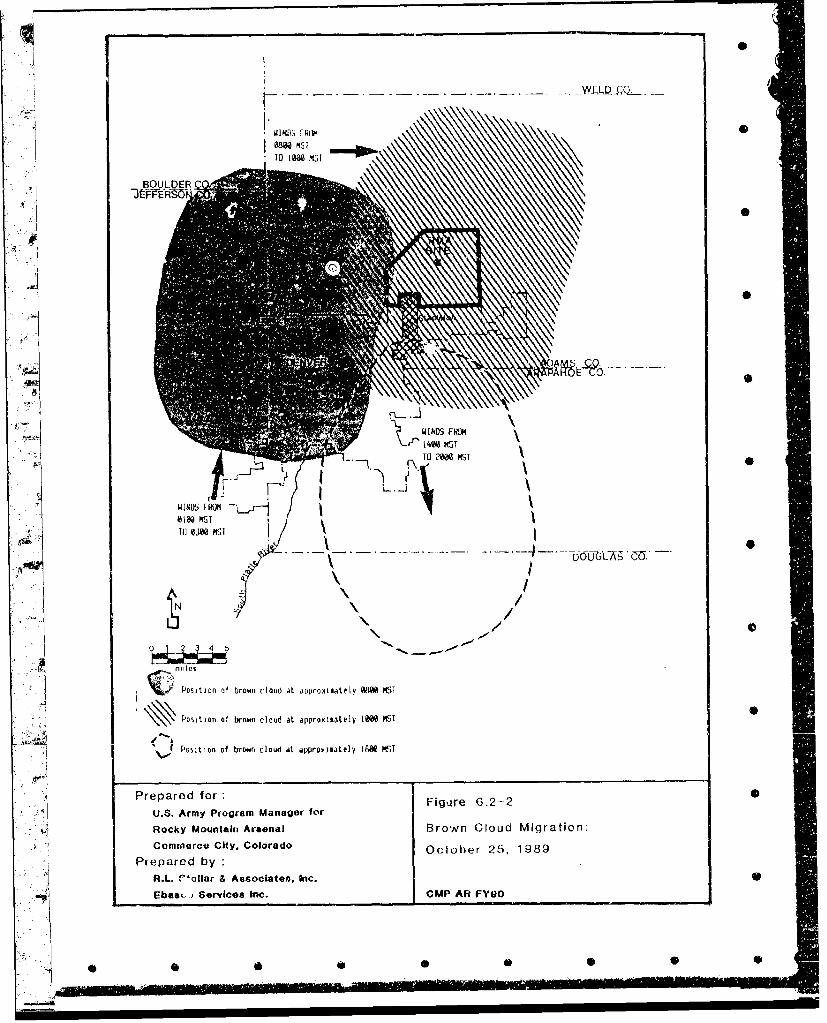
I ~ ~ WIND I~) RO

iD® 3L7 KS -

to lo .145BO L.DER

4ý/

WINDS F/140 S~To -m MST

Position~~~ ~~~~ ofboncoda ppoiaeyW iP

WINDS FROP161 ti0 ofbonMST tayniotl ~~PS

Position of brown cloud at approxisiately OMl MSTJ

Prepared for Figitre G.2-2U.S. Army Program Manager forRocky Mountain Arsenal Brown Cloud Migration:

Commerce City. Colorado October 25, 1989Prepared by

j R.L. f sillar & Associates, Inc.0Ebaao- Services Inc. CMIP AR FY90

- S 0 0 000

qdd ui XQN'DI' 4)0O> 0O

LU 0 j

Z~~' 0

Co 2\ CYLn~ aa)) O

c'Jcm

- 0 0.

g 00

U. 0 c

-0

- - 0

L()L

cm~ -9 -0)-.co~( E- co6a, o

00

a M 00 0g 0 2W .

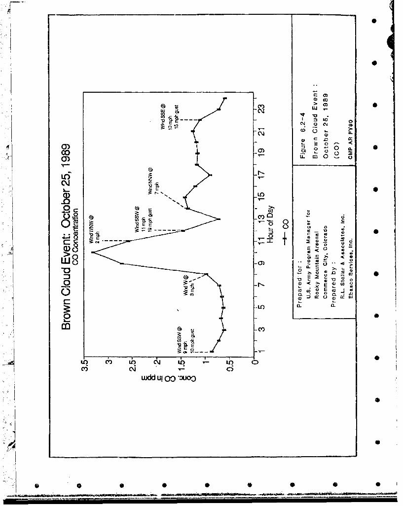
CQ)00

C') > C)w i CMJ w

I m U)

(DoCMJ

00 0)

c'Ju

0 0

00 0C

01 0

0 ccwI- - .6

E (a.13 ),O fl 0

cc0

ujda *i 0 -woo

L.

0

indicate the direct impact of both particulate pollutants and criteria gaseous pollutants from outside

sources upon the air quality of RMA.

January 5. 1990 •|_

The photographs for January 5, 1990, illustrate a typical winter day with an intense morning

inversion, which dissipated during the day and then reestablished itself during the evening hours;

Figure 6.2-5 illustrates this case. An interesting pattern was established between the wind direction

and the air quality throughout the day, as indicated by pollutant concentrations recorded at the RMA

"* continuous air quality monitoring site. When the wind blew from the direction of the brown cloud,

the gaseous air quality degraded. When the wind blew from the opposite direction, the air quality was

much improved. Table 6.2-2 presents the daily summary of gaseous pollutant and wind direction

data. Figures 6.2-6 and 6.2-7 also illustrate the concentration levels of representative pollutants for

the day.

In the early hours ef the day while the inversion was strong, the winds were light and from the south-

southwest to west. Concentrations of nitrogen oxides and carbon monoxide were noticeably higher

than normal at the RMA monitoring site during these hours. Coincident with a wind shift to the east-

northeast, these values dropped to more normal levels. When the winds again shifted back to the west

and southwest at the end of rush hour, concentrations also climbed again. At noon another wind shift

from the north--northeast was accompanied by a drop in pollutant concentrath ns for the remainder

of the day; wind speeds also increased significantly, signalling a break in the inversion and increased

mixing. Later in the evening, the winds shifted from easterly to southerly; also, the inversion was

reestablished. These new conditions coincided with the highest concentrations of the day.

In addition to the elevated gaseous criteria pollutant concentrations, considerably higher than normal

STSP and PM-10 concentrations were measured at RMA perimeter sites closest to Denver. AQI and

AQ2 on the western and northwestern boundaries both measured 72 ug/ms, while AQ5 on the

southern boundary measured 124 ug/m 3 . It is particularly interesting that in the previous example

(October 25, 1989), the western boundary stations measured the highest TSP concentrations with the~ ,.1..... • back ont the...Ar.nl..o

brown ....... back ontotheAr ffoioi the west and northwest. in this example, tile

advection was strictly from the south, and the southern boundary stations measured significantly

higher concentrations. This was also true for PM-10 levels on this date. Again, this case illustrates

t'.e direct relationships between Arsenal air quality conditions, metropolitan Denver influences, and

"pertinent meteorological factors such as wind speed, wind direction, inversion conditions and stability.

- 408 -

Rev. 08/15/91

---- -~- -~ ---

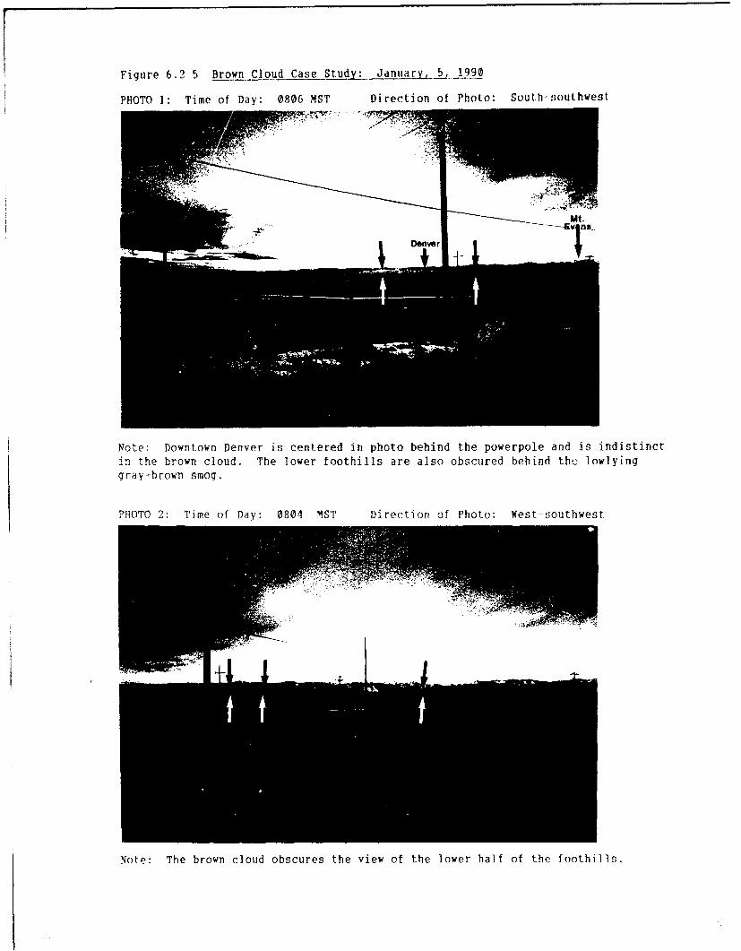
Figure 6.2-5 Brown Cloud Case Study: January, j5 990

PHOTO 1: Time of Day: 0806 MST Direction of Photo: South-southwest

Dever

Note: Downtown Denver is centered in photo behind the powerpole and is indistinctin the brown cloud. The lower foothills are also obscured behind the lowlyinggray-brown smog.

PHOTO 2: Time of Day: 0804 MST Direction of Photo: West-southwest

Note: The brown cloud obscures the view of the lower half of the foothills.

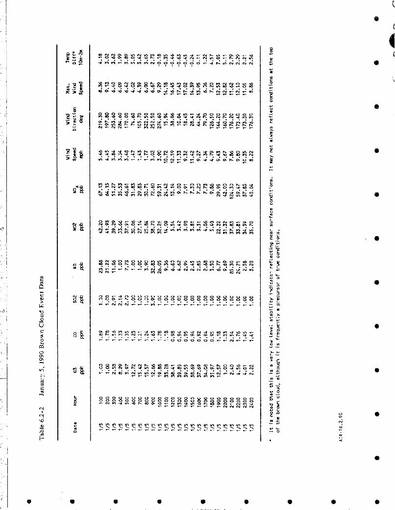
CýC

N00O1 1 aI OI 0 10 0 3m NO C1? 10V~ r-r '00N m

r t C)0 IChg C0t Q0 CUJ 0 CT

*! C% CC tV

-C1

"0 't It Cý"i n~ S0C' VitI I M~Z ~ on 0. -t 'r 0.0 No.003'ý g

t2 t :2:2 C cj a C'C) , Z8T, aft Ln -r Ar%.-o ýcýI 1 . .I- r~

0 0N' N.g

M It fn n C4 "-oo.I

0 n ; C u trgo03 ; MO. C-~~ J Cm C:)

C.

(Uo.n 0.0. t'ml tnto LA' 01n 1.13C N-N) r- CtoN 0 C> vi ) N o -t 't 00 'o Fnm n p- - In "J 4,

t~flffl fl N hn l CUj coM (%j 4

cli 0C*1'U)r 8 R2 ~ ~o-nU

rn~~ ~ ~ ~ ~ ~ ~ -- t V m I ' n I oL'9- 1' :.30 ý .

-*Jf C - - -t 0 C -i - - - C 0 03 0 0 C3 0ý 0D 0 4 0 0

C.

05 130fn)0>,P-P C 1 (

N- 0 l nt n 0 1G L 4I tt

onFonf np>

- ) lC : Q~ C)rU - a C) - a ao.0. g 0N-c aco... N

x .NIC"InQi0m 0.4t-t-c\N..tNrrr.-C MVMý

40.&ni Ai nt r i nL -% lL nLni n& %W n W

03 0

C~i 0

z0 0o

C 4

0- 0o S

LL m -

C: 6CI...

00 -

'- Eo 0

'c

Cal 0 Cd j .40LU r~~flt 00 l)i t

m CVL

qd U nO

CY)

qM ii -ou0

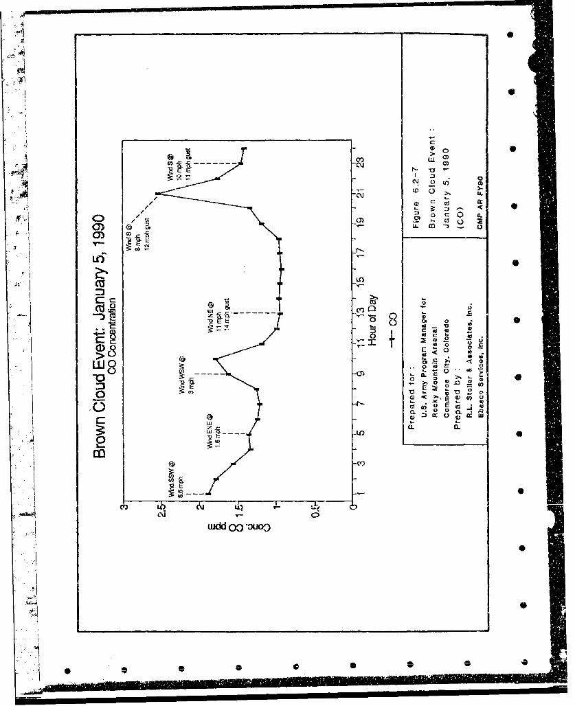
19

C)

o" a 0

CU 0' 0V)

/ *- 0/V

W8 0LI

o10:3

Cc Cu 0

C:)

-C9

Lb'I4 * 4.4o

2 L5=jembelr 14. 199Q

The morning of September 14, 1990, was a period of very poor air quality throughout the Denver

"metropolitan area, as well as statewide. Analyses of particulate samples in Devver and at RMA

showed the highest concentrations of particulates for the year at most sites. PM-10 concentrations

were also near their highest levels. Photographs taken on this day show a general, heavy haze of a

gray-brown tint, and very poor visibility (see Figure 6.2-8). The foothills cannot be seen through the

haze, and the downtown Denver buildings are barely discernable. All areas west of the RMA shown

in these photographs exhibit heavy visible pollution within the haze.

Septeinbcr 14, 1990, hias been documented previously in Section 4.2. This was a "limited mixing "day

j with an upper inversion capping the release of emissions from the boundary layer. Air quality was

not only poor in the metropolitan Denver area, but throughout eastern Colorado. Meteorological data

for the day indicate a dual level inversion; one at the surface, and thr otlier at about 8,000 to 9,000

ft (3,000 to 4,000 ft above the surface). The upper limit of the lower level inversion can be seen in

Photo No. 2 of Figure 6.2-8, which was taken facing to the north at about 0725 MST. This lower

level inN ersion likely contributed to the poor air quality at the RMA during the day, while the higherlevel inversion helped prolong the lower inversion.

Criteria pollutants monitored by the RMA continuous air quality monitoring site showed high

concentrations coincident with rush hour, and a wind shhit from southeast to southwest which brought

the flow from Denver directly over the Arsenal. Table 6.2-3 summarizes gaseous pollutant Lata and

pertinent meteorological data for September 14, 1990. Figures 6.2-9 and 6.2-10 illustrate pollutant

patterns for CO, SO, and NO, on this samoling day. (Unfortunately the NO. monitor was out of

service after 1100 MST.) Above normal pollutant levels were sustained until midmorning when"several meteorological factors began to change and hmlpiove the air stagnation pattern. As surface

heating continued, the low level inversion was broken, wind speeds increased and winds also shifted

to a northerly component. Also, the upper level inversion weakened, as reflected by the late

afternoon sounding for Denver. During the early evening, the surface inversion began to reestablish

itself and pollution levels began to climb again, particularly CO, as noted in Figure 6.2-10.

Of interest in this examp'e is that while gaseous data did not indicate excessively high pollution levels,

(although they were above typical morning rush hour values), very high concentrations of TSP and

PM-I0 were especially significant on this day. Concentrations on this particular day were probably

-413 -AIR- x.I 90.

"Re tv. 08/16/91

2flips

Bue628[rown Cloud1( (,Je 'St udr Sellte(II IIer 14, 11 ý110

PHOTn i: Timrie of Day: 0'125 MIST Direct ion (it Phorto: W es t s;u t IIwet w

Note:? Downtown Denver at, the left edge ot the photo, behind the powerpole, isrlvviý-ible. The Runiariani Flour Mill to the left of center, is indistinct in

The hal~:e. The foothillIs are virtualtv invisible, as are the mount ai s.

PHOTO 2: Timp of Day: 0~706 MST Direction of Photo: Northwest

N,!t~' The brown cloud obscures the foothills and appear,, as a broad hrowri handaIhovc lhe northern horizon.

-; tn-c mooz~-.'---ol -A - - -) - -- L

N-rflt-tN 0 00i~t04

Q CD Cý C Cý 3 C C5 ý Cý C3

C,- 0

0)

CU - c

m -0

K)~- LAl 4

--

I- C

rvnCn c Q N<dC- >Cfl wo~i Cn LnL m- 4 d K - C a >

(-' m. N ) 03 '0 w4(W

.2 00 C3

(9. (-rr a. C0) f C3- - ----. InJý- <3c4-'C 2C ) 0ma C

on w Pr m I- g 0' w C r" . - m w

""! .!4'!9 L!n 4:1 .1 11" 'tn C !9 C

n or 000 WN Pi-.-g'n gn

r -i

01 ~ ~ ~ ~ ~ ~ ~ ~ ~ ~ " 010 ýC ý0 lOl O ý C l olILco 0 '

+1iBrown Cloud Event: September 14, 1990

S02 and NOx Concentrations6O

W~WinW @W @

3mmph

40-

WS30-

8 wind SE @5

, /7"%,{. ~ ~Wind r~SW 0

10- • w,,JSE @ 0Wind NW @ 4 mph

/8mph 12 mph gust

/12 mph gust

1 3 5 7 91 11 13 15 17 19 21 23Hour of Day Not: NOx motor was out ofgr o u

at 1100 MST: S2 -4.- NOx

0

S...

,-: ' 1,Prepared for* rprdfr Figure 6.2-9


SRocky Mountain Arsenal Brown CIoud Event

Commerce City. Colorado September 14, 1990

Prepared by:RJ-. Stollar & Associates. Inc. (S02 and NOx)

Ebasco Services Inc. CMP AN FYO0

0 0'

AW

Brown Cloud Event: September 14, 1990CO Concentration

7mph 0

1Wind SW @

3 mph

.i: 0.8-

~~O6~~ WidW mph80.6" wM•NwO 11 mph gus Nu,0A; • 8 rnO

12 mph gustl" \

!{ 0.4-,

5 mph0.2-il '

1 3 9 11 13 15 17 19 21 23I tour of Day

••I *Q~c

4 -0



Rocky Mountain Arsenal Brown Cloud Event

Commerce City, Colorado September 14, 1990

Prepared byR.L Stoller & Associl'tes, In-(00

il Ebasco Services Inc. CMP AR FY90

I

0•"•i 0 0 S 0 0 5 0 0

affected more by trapped "particulate pollution" from limited mixing regional impacts than from local

gaseous pollution.

6.3 SUMMARY

This section has illustrated the interrelationship between visibility and air quality conditions at RMA,

and meteorological factors that control the transport of potential pollutants within the metropolitan

Denver area. Additional examples have been provided in Section 5.7 where emphasis was placed on

specific point sources that impact the Arsenal. There is no single or dominant parameter that can be

used to define or predict RMA air quality; however, multiple point sources and releases within the

metropolitan area have the potential to impact the Arsenal. There are also local RMA remediation

activities that have significance, depending upon the nature of the potential compounds which might

be released during excavation. There are, in all cases, overriding meteorological influences that

distribute potential pollutants both into the Arsenal and out of the Arsenal. In these studies, the CMP 0

is attempting to identify the variable sources and influences in order that air quality data measured

under the program can be evaluated in proper perspective.

0

J0,AIR90 .5-9 _•":'~Re.,,. 08/15•/91

i -

S....... i- .... -i - r

7.0 METEOROLOGY MONITORING AND DISPERSION MODELING PROGRAMS

7.1 METEOROLOGY PROGRAM OVERVIEW

The meteorological program and station locations are described in Section 3.5. A modification to the

program placed meteorological monitoring, maintenance and data processing and analysis under CMP

esponsibilities in FY89. Complete listings of all data collected and used in this report are provided

in Appendix J. Pertinent summaries of wind speed, wind direction, temperature, relative humidity,

barometric pressure, solar radiation, precipitation and stability are shown in the following sections.

7.1.1 PROGRAM OBJECTIVES

The meteorological assessment has several objectives. The first is to identify atmospheric conditions

associated with typical and potentially high contamination levels resulting from existing sources and

remedial activity at RMA. Prevailing wind flow, wind sr~eed, peak wind gusts, temperature and

precipitation all influence the release and spread of atmospheric emissions. A meteorological database

has, therefore, been established to identify typical relationships as well as to examine seasonal and

diurnal effects. For example, gusty winds often will cause higher levels of total suspended

particulates, inhalable particulates of less than 10 microns, metals and possibly semi-volatile organic

compounds. This information is pertinent to interpreting air sampling results. Certain pollutant

emissions may be more prevalent in summer than in wint.,r which may be an important factor for

* remediation planning. Also, diurnal influences (such as thie formation of a drainage wind pattern

* during nighttime and early morning inversion periods) will result in significantly higher levels of

certain pollutants. This information, again, is useful in assessing the potential spread of contaminants

and possible mitigating measures during remedial activities.

Another objective of the meteorological assessment is to determine the representativeness of the

meteorological data with respect to associated air quality conditions. Meteorological factors change

not only from season tc ';eason, but also from year to year. Variations in these elements, as noted, will

influence air sampling results. A particular sampling program, a period with anomalous precipitation

or- drought conditions, extensive snow cover, strong winds, very warm temperatures, or even generally

poor dispersion conditions will have a direct influence on pollutant levels at specific monitoring site

locations. Again, this information is essential for interpreting the results. Consequently, this

meteorological data will be useful in assessing remediation progress over the total period of the CMP.

- 419 -

. AIR - 9.5-9

Rev. o8/11/91

"• _,it•Im • .- ........--.. --,--* "" --- '•.--., " ..........----.. . • •: • -:'- . ..... .:' "•-•• --• '•.- _ . - - - - - - - - -

In addition to the above factors, the meteorological program directly supports air quality model

applications that are used in pollution dispersion evaluations and predictions. These, in turn, are

employed for assessing impacts beyond the RMA boundary, or in predicting real-time pollution levels

during remedial activities.

ar7.1.2 DATA RfOVbRYd g

Details of the recovery of FY90 meteorological data for each parameter of the composite database areS given in Table 7.1- 1. Recoveries are based on the total number of hours of possible data during the

period October 1, 1989, through September 30, 1990 (8,760 hours). Temperature difference wias not

started until November; therefore, the total hours possible was 7,807. Observations (hourly values)

were considered invalid or missing if there were less than 45 minutes of valid recorded data for that

parameter or if there were equipment malfunctions or calibrations.

Table 7.1-1 Summary of RMA Meteorological Monitoring for FY90

Parameter No. Samples % Recovery

Wind Speed 8,734 99.7Wind Direction 8,734 99.7Sigma Theta 8,734 99.7

Temperature 8,760 100.0Relative Humidity 7,814 89,2 4Barometric Pressure 8,29r, 94.7Solar Radiation 3,76oJ 100.0Precipitation 8,'o 100.0Maximum Gust 8, " 99.6Temperature Difference

(10 m - 2 m) 98.6Stability &' 34 99.7

Program Total 93,748 98.3

S

7.1.3 DATABASES

A single, representative composite database was developed from data collected at all four RMA sites.

Site M4 was the primary source for the composite database for all of FY90. Data from other sites 0

were also used to fill in or substitute for the invalid or missing data. The amount of substituted data

- 420 -" ' .11AIR-90.5 -9

Rev. 08/15/91 0

* . .S........ . ... .. •.

is generally very small (3 percent or less). Certain parameters are taken from different sites for the

9 1 composite database since no site monitors all the parameters. Relative humidity, maximum gust andJ 'temperature difference (10 m - 2 m) were from MI, and solar radiation was from M2. All other

"meteorological parameters were obtained from M4. Complete listings of the composite database and

the associated joint frequency distributions used for this report are provided in Appendix I. The

composite database provides a suitably representative sample of meteorological conditions at RMA

for FY90.

Separate databases were also maintained for each site (MI, M2, M3, and M44) without any

substitutions being made for missing or invalid data. These databases were used for site comparisons

within the Arsenal boundary to note any areal differences. The joint frequency distributions for each

site are provided in Appendix J.

All summaries shown in this report were prepared under the CMP and taken from the FY90

composite database, except for the comparison of the four meteorological sites (Section 7.5) which

utilizes each of Ihe separate databases. All data have been thoroughly checked for quality, including

7, the substituted data. Long-term climatological Denver Stapleton Airpert means (Section 2.2) were

used for comparison. The FY88 and FY89 data, which were also used for comparison, are provided

in Section 5.0 of the FY88 Air Quality Data Assessment Report (Stollar, 1989) and in Section 6.0 of

the FY89 Air Quality Data Assessment Report (Stollar, 1990). Pertinent summaries of all of the above

parameters follow.

7.2 IJMMAIIY O' IRESULTS

A summary of monthly and annual (October 1, 1989, through September 30, 1990) meteorological daw

for FY90 at RMA is provided in Table 7.2-1. All parameters summarized in this table are based onhourly averaged values with the exception of maximum gust, which is the maximumn instantaneous

wind speed for the period. Maximum speed is the maximum 1--hour average wind speed value for

the period. The predominant wind direction indicates the sector (of 16 possible sectors) ftrom which

the wind is blowing most frequently during the reported period. Temperature difference is the

difference in temperature between the 10-meter and 2-1neter sensors (1 0 m - 2 mn).

The monthly means and extremes of temperature values clearly depict the typical annual cycle, with

only minor deviations from normal. The precipitation data revealed an annual cycle, but it was

somewhat masked by individual events. The spring season was drier than normal while the summer

-421

AIR-90.5-9nev. 08/15/91

0 • 0 0 0 0 0 0

I •

-

.0

0a 0 -X40 -d a\O0\4 -6

So .2o'C' o-. --0 00000r'Joo- ý4 -0Cft'~rQEd c, D

,-

r.0-

000

C> al' "'T 00,r' r- C \0 CDo o -o 7. a,, o,, ON- o,,-•~ .. .. ..- . . . . . . . . . ..

cd p( c )C

0 o Mooo oooooo

H.P r6,-09--. C.-:

-IIt

0

Cie0

< CD

04 0• ON, (n -- (N, -- 00 ,1) \.D oC -,,-.,

onoa

0cu

r-*iD(f at--C ' r-nt M o t- 0-0'T Cy

o . . . . . . . . . . . ..iCU

Cd 4)

z a

kA W.0 00 W -4% t-r

4) --- - - - -

a, I00

0% u4)C n% I D0 % t' nG

V ) -ý 4 ) O ' n In . ' t f 'n I ar

W- .- 0 t ný 0 nr W0%

4) JzL.

0 00

l Vý W3 Nlt l O 04 C Ci 0N'N f

0

4)

n~nc'' t~o..~ -2ri :I0

1. w 0

0 0U

01) %0V D )--001 4 T

I) a1- 00 c.0 C>I ')11-Z

4) a) W5 .0 u >

Z0 E.0t ,R a c c 4) El tsz 4-06. Go cZo 00O G fla ON0 0 0 -

rnCIS

00)

.0 QCI CAt 0n-n% -00a o C4I

4.w0

0

was moist. Wind speed data showed the strongest winds during the spring months, but the maximum

gusts were c!early dominated by single events. The predominant wind direction during FY90 wasfrom the south-southwest, which was slightly different from the expected prevailing pattern ofsoutherly winds. Stability patterns showed a maximum of stable conditions in the fall and winter and

a maximum of unstable conditions in the spring and summer. A neutral stability condition prevailed

during all months with almost half the total frequency of occurrence.

The parameters are discussed in more detail below. Included are discussions of FY90 conditions in

comparison to FY88 and FY89 data (where applicable) and to the long-term climatology at Stapleton

Airport. Also, specific conditions, extreme events, and anomalous conditions are described for eacht

parameter.

7.2.1 TEMPIeRATUR1,

The RMA FY90 annual mean temperature, 50.6'F, was very close to normal. The year itself was near

or slightly warmer than normnal with only minor deviations. The summer months of July and August

were somewhat cooler (4.4°F and 1.71i blow normal, respectively) associated with increased rainfall.

January was somewhat warmer at 6.71F above normal. The maximum monthly average was 71.81F

in June and the miniimum monthly average was 27.71i in December. The maximum temperature,

98.6 0F, was recorded in June during a short heat wave, and the minimum temperature, - 14.01', was

recorded in December during a cold wave. This cold wave came in December as opposed to Iebruary

in FY89. The time series of daily maximum and minimum temperature through the FY90 program •

is shown in Figure 7.2- 1, indicating the extreme events and the day-to-day variability in temperature.

7.2.2 RELATIVE I IIMIDITY

The annual mean relative humidity, 52 percent, was near normal. All months followed quite closely

to normals with higher values in the winter and spring due to lower termperatures and increased

amounts of precipitation, and lower values in the summer and fall due to higher temperatures. The

maximum monthly average was 65 percent in April and the minimum monthly average was 39 percent

* ill October.

- 424 -

AIR -90.5 -9 00 ,. 08/10/91

;~4 • 4••9

CuX

Us 0 co

C'J = 0) CDc- -u

i U- cr

0 0 0

41 O 'E000 C '

CLL

E

o 0

o a' co t- 40 ki V r2 F4 -4 N

* IQ)

0

J 7.2.3 BAROMETRIC PRESSURE

The annual mean station barometric pressure, 24.71 inches of mercury (in. fig), was almost identical

to long-term normals. All months followed the normals quite closely. The maximum monthly average

was 24.82 in. Hg in September and the minimum monthly average was 24.61 in. Hg in January and.1 May. 0

7.2.4 SOLAR RADIATION

The solar radiation values included nighttime values to show the increase in solar radiation in the

spring and summer due to the length of the days. The annual mean solar radiation was 0.29 langleys

per hour (ly/hr). This value was higher than that of FY89 (0.24 ly/hr). Values were slightly higher

in the summer with lower values in the winter. The maximum monthly average was 0.49 ly/hr in

June and the mininmum monthly average was 0.13 ly/hr in December. The RMA area generally has

an abundance of sunshine throughout the year, as was evident in FY89 and FY90.

7.2.5 PRECIIITATION

Precipitation for the l"Y90 period from October 1, 1990, through September 30, 1990, totaled 11.56

inches at RMA, compared with the climatological mean of 15.31 inches or 3.75 inches below normal.

Stapleton Ai lport data for FY90 was much closer to normal. The lower amount at RMA may, in part,

be due to winter readings, when snow blows away before it can be measured. The spatial variability

associated with summertime thundersturm activity may also account for this difference. I)uring the

colder seasons, precipitation was primarily in the form of snow with a total of 62.2 inches falling in

55 days. A major snowstorm occurred on March 6, reflecting the elevated total of 1.97 inches of

precipitation for that month. The heaviest monthly precipitation total, 2.58 inches, was measured

during July. The month of May generally records the heaviest precipitation, with a long-term mean

of 2.47 inches and an all-time maximum of 7.31 inches. Hlowever, in FY90, summertime heavy

precipitation events accounted for higher levels in July and August; several storms were intense and

stagnated over the area, allowing the majority of the monthly precipitation to be recorded in I or 2

days.

The rest of the FY90 monitoring period was normal to drier than normal. The driest month was

November with only 0.03 inches. A time series of daily total precipitation during the FY90 program

is shown in Figure 7.2-2. Heavier precipitation events in the spring and summer are highlighted.

- 426 -

AIR-. 0/.5/-9"' ItRev. E8/15/91

S 0S0

. jr

Daily Precipitation Values

1--

U.8

0.7 0

0,6

U.• • 0.5

0.4

0.3 -

0.2

0.1

Oct. Nov Dec• Ia Feb Mar Apr May Tun Jrul Aug Sep

Month

Prepared for:SU.S. Army Program Manager for Fgr .-

Rocky Mountain Arsenal RMA Graphicai Depiction of PrecipitationCommerce City. Colorado

• .- • Prearedby :(Oct. 1, 1989-Sept. 30, 1990) •

R.L Stollar & Associates. Inc.

Ebi4sco Services inc. CMP AR FY0.

-l

I _SS SS_

Also, it can be seen that total monthly precipitation was often a reflection of one or a small number

of heavy rainfall events.

7.2.6 WINDS

Hourly mean wind speeds for the entire CMP FY90 program averaged 8.6 mph compared to a 30-year

climatological mean value (at Stapleton Airport) of 8.8 mph. This close comparison is important

because pollutant levels, especially those associated with dust particles (i.e., TSP, PM- 0, metals and

SVOCs) are sometimes generated by high wind speeds. The data show that FY90 mean, wind speeds

were close to average for all months. The maximum monthly average was 9.9 mph in June and the

minimum monthly average was 7.5 mph in September. The maximum gust, 52.8 mph, was recorded

in MWy. The predominant wind direction for the RMA in FY90 was south-southwest, compared to

the Stapleton Airport 30-year record of south. In FY90, the RMA had a predominant south-

southwest wind for all months except July, when the predominant wind was from the south. During

FY88 and FY89, predominant winds were more variable from month-to-month; however, the long-

term normal was southerly. As noted in Section 5, the slight shift of predominant winds at RMA in

FY90 from south to south-southwest may have accounted for slightly higher criteria pollutant levels

at RMA. The time series of daily mean wind speeds, maximum gusts, and predominant wind

directions during the program are shown in Figure 7.2-3.

There was a slight disparity between the 5-yea, seasonal and annual wind roses for Stapleton Airport

and the coiesponding wind roses for the CMP FY90 monitoring periods shown in Figures 7.2-4

through 7.2-8. 1 fhe CMP FY90 wind roses showed lendencies for a strong south-southwest to north-

northeast flow, whereas, south to north is the most common flow pattern at Stapleton Airport. The

secondary component was north- northeast at RMA, compared to northerly f'or the long-term normals.

The FY90 wind patterns w,,re close to normal patterns in all other directions.

7.2.7 ATMOSPlHERIC STABILITY

Atmospheric stability is an important 1rarameter relating to the dispersio,. of air pollutants. Along

with wind speed and wind direction, it is a key parameter in air quality dispersion models and reflects

the potential of the atmosphere to diffuse pollutants horizontally and vertically. Table 7.2-1 shows

the frequency distribution for all atmospheric stability categories A through F during the CMP

monitoring period. A full joint frequency distribution (IFD) of wind speed, wind direction and

stability is provided in Appendix J. Catego, ies A, 13 and C, which indicate good dispersion or

- 428 -

Alit 90.6 9Rev. ()8/15/91 0

• 0 • 0 • • 0 • 4

IO

Daily Wind Speed Values FY90(Maximumn Gusk. )ivau Speed)

60

'50

40SS

a0-2o -

ULt Norv Dc Jan Feb Mý Apr )bq Jun Jul Aug Sep

IthnUi

Daily Predominant Wind Direction FY90

4 - - f + 4 +- + + 4.

+ 4 + + +- +- +4 .÷-44- + 44-+. + 4-4-+-4.

F + t t 4- -t r - if -t + 44 1

300

+4+4 4+ 4 4 -4+ + + 4 4- +•.+ ÷4 4 • •4, + +. 4. + 4S250- 4- * 4- 4- 4- -4

- I f - W t i-5 0t f t f i +4 4-, 4--i- O + 4+ - 4- ++-# I- 4-ttH-i*$4*0 4-3 -* 1tt -4. -*44-1-H~ lif -44-t4+t -fl- 4- -4 tif t- + 4- 4- U•4-- t- tI+ 4-tUI++4--4.•

+ 44- + + -it +" t + -t I +-ff f4 -t -44-f+1""I+-+

v 10 4.4+ 4 4 44- 4 + +4-4- + + + +

1 4:) 4- ++ +4- 4 44. * ÷4

+0 , + 4- 4 4- + t 4- t + . f -

+ +- 44 4 + 4 - ++

50 + 4-- 4-4.4- 4- + -0

1 4- ++ +4 4- 4- 44- -i- -W 444 4-1- +- 4

Oct Now Doc Jtan Fab ]Xa- Apt Ma J-n J.1 Aug Se.p

Prepared for :Figure 7.23

U.S. Army Program Manager forRocky Mountain Arsenal RMA Graphical Depiction of

Commerce City. Colorado Wind Speed and Wind Direction

Prepared by (Oct. 1, 1989-Sept. 30, 1990)R.L. Stollar & Associates. Inc. •

Ebasco Sorvlce8 Inc. CMP AR FY00

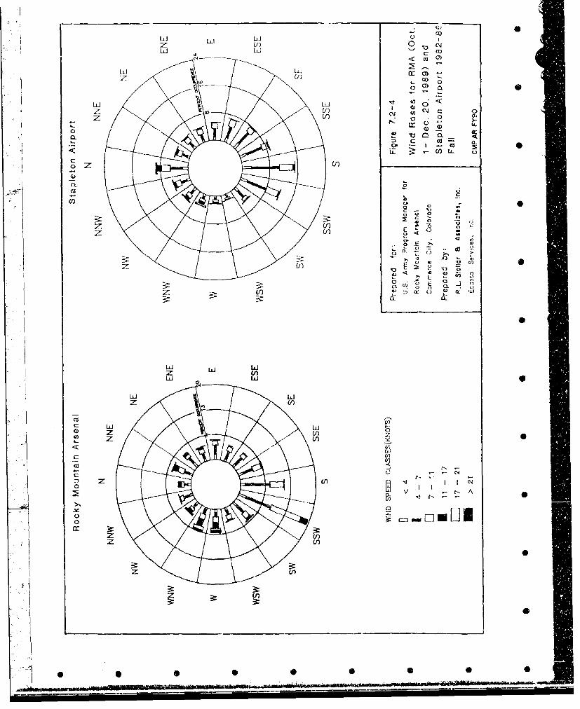
Lii Ld I

wL Lii

z 0

CC

0 . >

C12L

-L 0) 0

0 dID;.

AD• Id

s..2

z SUe0 0

En w ) L6

4:L

LLU)CU(CL

, .-

ZMt

L0A ,j- N0'-

U)

00

Z V)

V)0

jijz S 000

L iL LI CL )LO

LII Li 0

111 C 0

z 0 oCD )

co ~N '- o U.

oC '

z (i-

U) c)

(r. IL ) Wi

LU Li

IdLLLi Liz z)

C-

0N

El- v0

C:3 f

o3_1

-,Mao

_L SL L

UJL

wl LIL -a)

(10 0) c

o

oD U . CLJ

I-a L < 04 9 f(n . ca c

V)CCU

0 V)

0W

00

SU) 0-r

z f

CUl

Li L

z ccJz V)

0 C=3

zz

U)S

07ý1 I

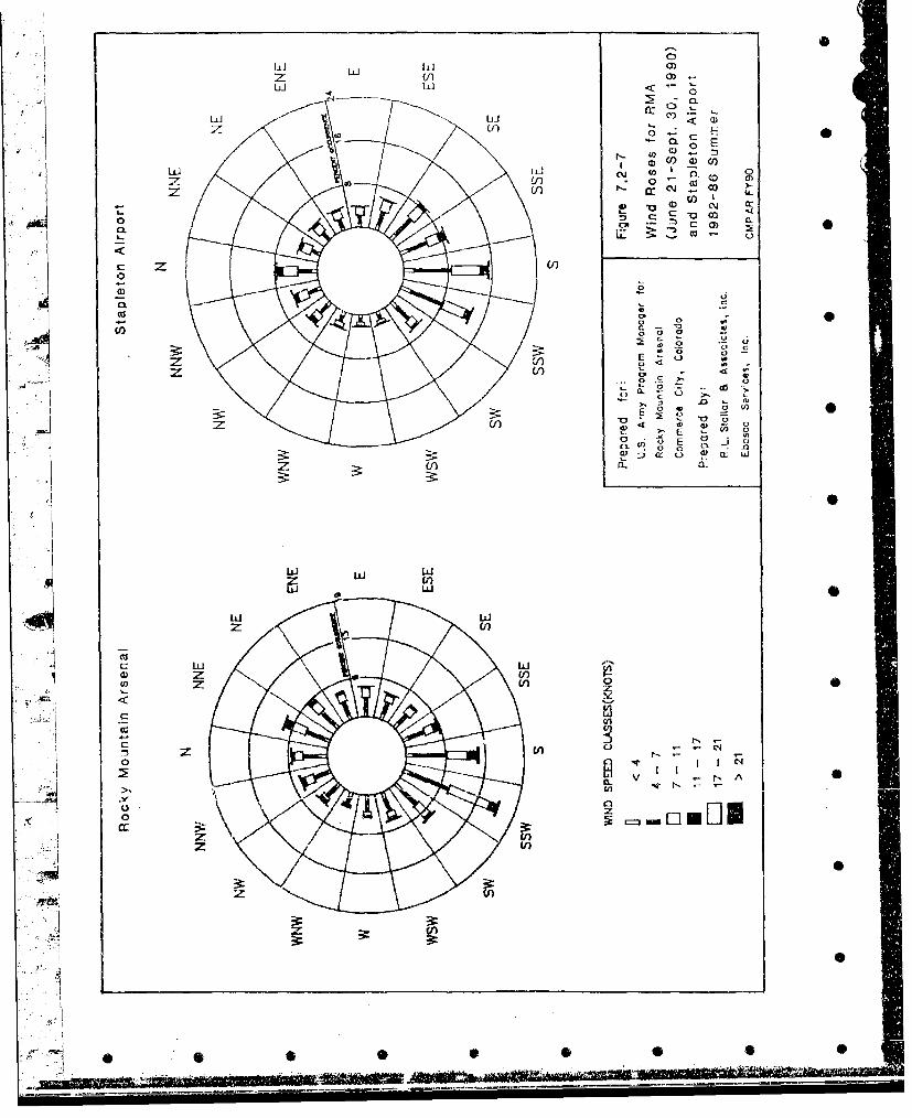
0~~

11.c zu0

,*& CL-51ý

00

cxV

CU 0 .-L

0E

wd w "

LLi

z L Lz

CC

0 A

.~ .- .. ..

LU J w ~LUJ LUJ C' 3

C4~~ -: :LUJ LUi4z (I) 'a co

z OD- 0)!

LLU

00 130)as

00

0r w

-j 0z -n

CoILA

4)j w )~

4-i L.

z Co

Cd

EI N

0 z

0z

0 0 9 0 -'

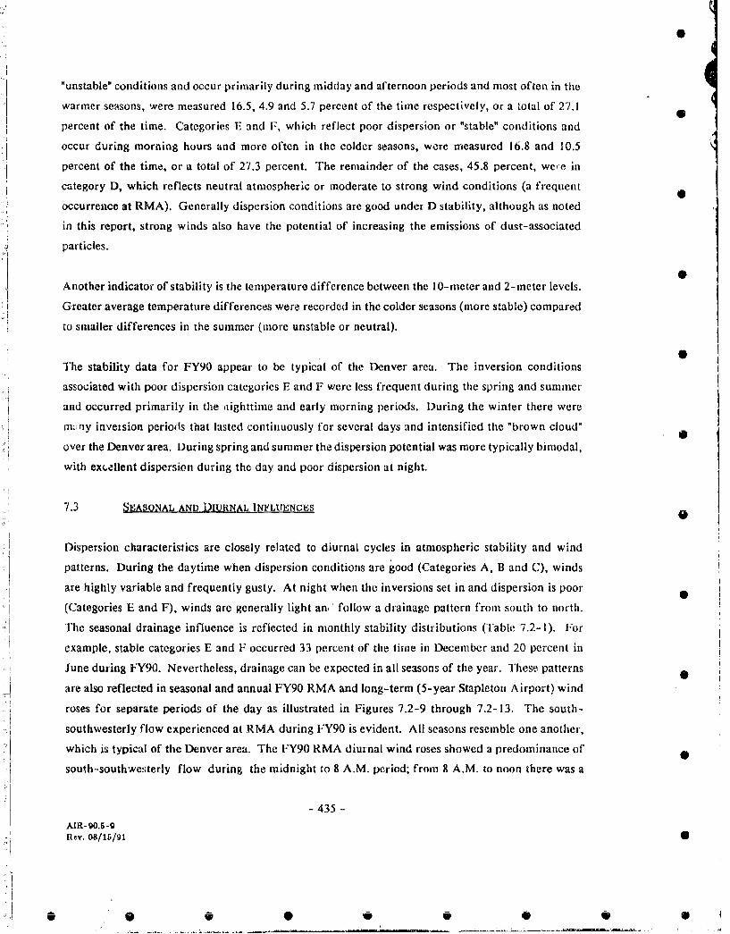
"unstable" conditions and occur primarily during midday and afternoon periods and most often in the

warmer seasons, were measured 16.5, 4.9 and 5.7 percent of the time respectively, or a total of 27.1

percent of the time. Categories E and F, which reflect poor dispersion or "stable" conditions and

occur during morning hours and more often in the colder seasons, were measured 16.8 and 10.5

percent of the time, or a total of 27.3 percent. The remainder of the cases, 45.8 percent, wc,-e in

category D, which reflects neutral atmospheric or moderate to strong wind conditions (a frequent

occurrence at RMA). Generally dispersion conditions are good under D stability, although as noted

in this report, strong winds also have the potential of increasing the emissions of dust-associated

particles.

Another indicator of stability is the temperature difference between the 10-meter and 2-meter levels.

Greater average temperature differences were recorded in the colder seasons (more stable) compared

to smaller differences in the summer (more unstable or neutral).

40The stability data for FY90 appear to be typical of the Denver area. The inversion conditions

associated with poor dispersion categories E and F were less frequent during the spring and summer

and occurred primarily in the aighttime and early morning periods. During the winter there were

Sm:jrly inversion periods that lasted continuously for several days and intensified the "brown cloud"

over the Denver area. During spring and summer the dispersion potential was more typically bimodal,with ex(,allent dispersion during the day and poor dispersion at night.

7.3 SEASONAL AND DIURNAL INFLUENCES

Dispersion characteristics are closely related to diurnal cycles in atmospheric stability and wind

patterns. During the daytime when dispersion conditions are good (Categories A, B and C), winds

are highly variable and frequently gusty. At night when the inversions set in and dispersion is poor

(Categories E and F), winds are generally light an, follow a drainage pattern from south to north.

The seasonal drainage influence is reflected in monthly stability distributions (Table 7.2-1). For

example, stable categories E and F occurred 33 percent of the time in December and 20 percent in

June during FY90. Nevertheless, drainage can be expected in all seasons of the year. These patterns

are also reflected in seasonal and annual FY90 RMA and long-term (5-year Stapleton Airport) wind

roses for separate periods of the day as illustrated in Figures 7.2-9 through 7.2-13. The south-

southwesterly flow experienced at RMA during FY90 is evident. All seasons resemble one another,

which is typical of the Denver area. The FY90 RMA diurnal wind roses showed a predominance of

south-southwesterly flow during the midnight to 8 A.M. period; from 8 A.M. to noon there was a

- 435 -

AIR-9O.6-gRev. 08/1S/91 6

U B B 0 U

0ROCKY MOUNTAIN ARSENAL DIURNAL WIND ROSES

C 1-4 mat) ( 4-S n.t) (0-i' Me

(12-15 n1.t (i1-20 mrn) (20-24 mM)

DENVER STAPLETON FALL DIURNAL WIND ROSESFrom 1982 ,- _•(..m(" -,

%Oxox ox

ox

(12-16 met) (16-20 -t) (20-24 m.t)

S~Prepw]ed br :U.S. Ar g Program Manager for

Hocky Mounlain Arsenal

Cowonfore .ffy, Colorado

Prepared byR.L Stallar & Amtietu.l Inc.

Ewoew "4Vices, imc.

Figure 7.2-9

RMA and Stapleton Airport

Fail Wind RoseComparisons S

CMP AR FY90

a a a - •

ROCKY VtOUNTAIN ARSENAL DIURNAL WIND ROSES

. 1-4 .. t) (4-8 m.0) (8-12 et

0

(12- 8 m.) ( 1I-20 nmi) (20-24 m..)

DLNVER STAPLLTON WINTER DIURNAL WIND ROSESFrom 1982 -1986

xI

(1-4 n.t) ( -- , (B-12 -. t)

oxx

0"0

(12-8 11-t) (18 20 -r t) (20-24 -tM)

SPrepared for:

U.S. Army vrogrom Mcaogwr fo,

Rocky¥ Moun8,i. Asr*uI

Comim.Ot. Cy. Colorado

Prepared by:ft.L. SIoNw & Associaels. Inc.

Figure 7.2-10


Winter Wind RoseComparisons

_ __ __ •CMP AR FY90

0 I

ROCKY MOUNTAIN ARSENAL DIURNAL WIND ROSES

(1- m.o) (4-6 w.t) (a-12 .mipt

*-OO(12-16 ,i..t (16-20 ",A) (2G-24 moot)

DENVER STAPLETON SPRING DIURNAL WIND ROSES

ox -Ox

1 4)1

ox OX

02 'Ox(1--4 r1 .t) (14-2 ri.t) (20 n,-2A

02- -014 --- \

Preparejd b0:

U.S. Army Program Munagtr fot

R.u;1y Muunk.ui Ar4...m

Commt-crc City, CoIorudo

Prepared by!R.L. Stoallw & Aslasoft.., In-.

Figlue 7.2- 11

RMA and Staploton Airport

Spring Wind Rose

Comparisons S

_____CMP AR FY90

.. .. -. - - - -- --- .. ----

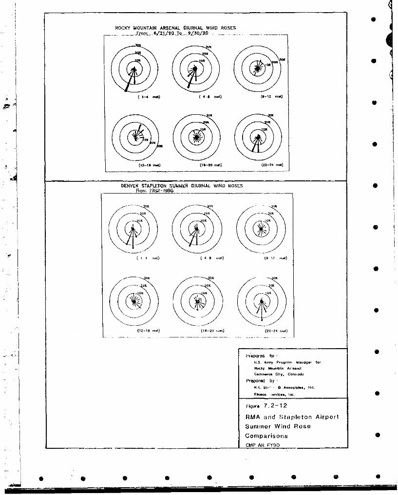
0

ROCKY MOUNTAIN ARSENAL DIURNAL WIND ROSES- ... . --- f°ro '-"6 /'J-llT-•q-'9L3QL•- .. . . . . .. . .

(1-4 rn"t) (4-20I wt) (20-2 r*1)

DENVER STAPLETON SUMMER DIURNAL WIND ROSE5Fon 1962-1986

"1- 4 '-t) 4- ,.t)

oN ox

(12-19 ,,,Q0 (116-2 ,0 ,t) (20-24 ,,.t)

-0te2ad for:

U.S. Army Progfon, MaolOg*,r for

Rocky Moun•lIn Arlol

Cumnlw" Cty, Color,*&

Prepored1 by:N.L.$S•," r 8 A4,cI9,Ote , Inc.

Ebo •co .- vkoi, IC. I

Figure 7.2-12

RMA and -tapleton Airport

Summer Wind Rose

Comparisons 0

CMP AR FY90

0

ROCKY MOUNTAIN ARSENAL DIURNAL WIND ROSES

(1-4 M)3 4-8 nWQ (8-I 2 -4t)

DENVER SIAPLETON ANNUAL DIURNAL WIND ROSES0From- 1982-198lG____

0- ox

A00

( 2 0 ,,.~)(16-20,-t1) (20-24 .nut)

Prepured for

U.5 A-ny P-ogl-x Monw2..- (-II ~ Roky mounloin A,94001Con,"'." Cy, colo,U&4

Prepaured by

l~boooo S.rvic"-. Inc

Figure 7.2 -. 13


Annual Wind Rose

Corn par iso n S

_____________ ___________________________CMI AN FY'90____

slight transition, but southwesterly flow still prevailed; from noon until 8 P.M., however, winds were

highly variable, with perhaps slightly more flow from easterly components; 8 P.rA. to midnight was

a transition period, with the winds beginning to shift from southeast back to south and south--

southwest.

The representativeness of the FY90 diurnal wind patterns is illustrated by a close comparison with

the long-term diurnal wind roses. FY88 and FY89 diurnal wind roses were also comparable to the

long-term diurnal patterns.

7.4 SUMMARY AND CONCLU$IONs 0

Although mean weather patterns change from year to year, it appears that the FY90 meteorological

data, with minor differences, were representative of long-term data and provide a useful instrument

for assessing contamination impacts during this period and for future remedial progress evaluations.

Table 7.4-1 provides a comparison of FY90 meteorological parameters with those of FY89. The only

differences of note were a shift in the predominant wind direction from south in FY89 to sov,,h-

southwest in FY90, a maximum wind gust of 72.5 mph in FY89 compared to 52.8 mph in FY90, ai,'

a solar radiation level of 0.24 ly/hr in FY89 compared to 0.29 ly/hr in FY90. The solar radiometer

was out of operation for a period during the summer of 1989, which may account for the annual

differences for that parameter.

The data also suggest important guidelines for mitigation thw may be appropriate during remedial

activities. Emissions from daytime activities would contribute lesser impacts than nighttime and early

morning activities because there are better and more variable dispersion conditions during the day.

At night, inversions are prevalent and dispersion conditions are poor. Also winds at night are

channelled north and noithtast of the remediation source. A factor that should be taken into account,

therefore, is the distance from a remediation source to sensitive areas north of the Arsenal, such as

public roads and residential areas beyond RMA boundaries. However, dispersion potential apparently

decreases significantly with distance from a ground emissions source and depends upon meteorological

conditions.

In this section, typical impacts were inferred based on seasonal and diurnal meteorology. For real-

time applications or for short-term and long-term assessments, these influences must be incorporated

into atmospheric dispersion models along with detailed source emission characteristics. Model

-441

AIRCl0/.5-9R~ev. o8/is/,al

.. I= - * ~ ~

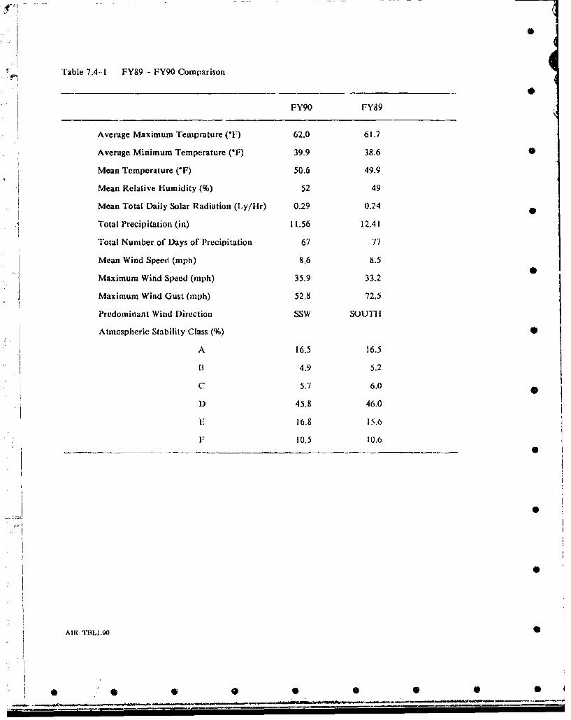
"Fable 7.4-1 FY89 - FY90 Comparison

FY90 FY89

Average Maximum Temprature ('F) 62.0 61.7

Average Minimum Temperature (*F) 39.9 38.6 0

Mean Temperature (*F) 50.6 49.9

Mean Relative Humidity (%) 52 49

Mean Total Daily Solar Radiation (Ly/Hr) 0.29 0.24

Total Precipitation (in) 11.56 12.41

Total Number of Days of Precipitation 67 77

Mean Wind Speed (mph) 8.6 8.5

Maximum Wind Speed (mph) 35.9 33.2

Maximum Wind Gust (mph) 52.8 72.5

Predominant Wind Direction SSW SOUTII

Atmospheric Stability Class (%)

A 16.5 16.5

4.9 5.2

C 5.7 6.0

D 45.8 46.0

F 16.8 15.6

F 10.5 10.6

A *

AllR TBLA.00 0

0 9 9 S • • 0

approaches employed in the present report and recommended for future remedial progress evaluations

are discussed in Section 7.6.1. 1

. 7.5 RMA MAETEOROLOGICAL STATION COMPARISONS

During FY90, at the request of PMRMA. a special comparison was made between the data compiled 0

at the four meteorological stations operating at RMA. Figure 3.5- 1, previously shown, indicates the

locations of these stations. In general, the terrain across the Arsenal is fairly uniform. Nevertheless,

"there are slight differences in elevation and surrounding topography that could affect air quality

dispersion characteristics on certain occasions. Met Station 4 is the highest station located on the crest 0

of a knoll at 5,278 ft. Met 1, just to the cast of the old Basin F, is the lowest station at an elevation

of 5,192 ft. Met Station 2 located to the north of North Plants is at an elevation of 5,193 ft, but

separated from Met 1 by higher topography. Met Station 3 is located southeast of Basin A and

northeast of the South Plants at an elevation of 5,263 ft. Channelling of winds around topography 0

and temperature differences, due to drainage and elevation differences, are the main variations

between the sites. (Met stations I through 4 are identified as MI through M4 in Figure 3.5-1.)

Tables 7.5-1 through 7.5-3 provide a comparison of the four stations for wind speed, wind direction, 0

temperature and precipitation from February 1989 (when the meteorological program under CMP was

initiated) to the conclusion of the FY90 period in September 1990. It should be noted that certain

periods of data are missing or invalid due to calibrations or tower work. These data were not included

in the tower summaries. Also, the temperature sensor at Met Site I has a tendency to be slightly

warmer due to the sensor construction; Table 7.5-2 indicates temperatures at Met I were an average

of ITF higher. Overall, only minor differences were noted between the stations.

The highest average FY90 wind speed of 8.7 mph occurred at Met 4, which is at the highest elevation S

and is the most openly exposed station in the network. The lowest average FY90 wind speed, 7.6

rmph, was at Met 3. Average FY90 wind speeds at Met I and Met 2 were 8.2 and 7.9 mph,

respectively.

J iThe predominant wind direction at all stations was from the south-southwest with the exception of

Met Station 2 where the predominant wind direction was from the south. This is a reflection of the

slightly higher topography to the southwest of Met 2, illustrating how very modest topography

differences can impact wind flow patterns. Channelling of winds around this terrain often results in •

winds from the south rather than southwest at Met 2.

- 443

AIRt.90.5-9Rev. 08/1i/91

S 00 00 00

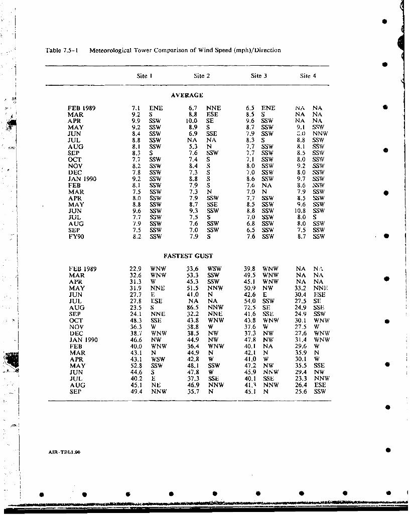
Table 7.5-1 Meteorological Tower Comparison of Wind Speed (mph)/Direction

Site I Site 2 Site 3 Site 4

AVERAGE

FEB 1989 7.1 ENE 6.7 NNE 6.5 ENE NA NA 0MAR 9.2 S 8.8 ESE 8.5 S NA NAAPR 9.9 SSW 10.0 SE 9.6 SSW NA NAMAY 9.2 SSW 8.9 S 8.7 SSW 9.1 SSWJUN 8.4 SSW 6.9 SSE 7.9 SSW S. 0 NNWJUL 8.8 SSW NA NA 8.3 S 8.8 SSWAUG 8.1 SSW 5.3 N 7.7 SSW 8.1 SSWSEP 8.3 S 7.6 SSW 7,7 SSW 8.5 SSWOCT 7.7 SSW 7.4 S 7.1 SSW 8.0 SSWNOV 8.2 SSW 8.4 S 8.0 SSW 9.2 SSWDEC 7.8 SSW 7.3 S 7.0 SSW 8.0 SSWJAN 1990 9.2 SSW 8.8 S 8.6 SSW 9.7 SSWFEB 8.1 SSW 7.9 S 7.6 NA 8.6 SSWMAR 7.5 SSW 7.3 N 7.0 N 7.9 SSWAPR 8.0 SSW 7.9 SSW 7.7 SSW 8.5 SSWMAY 8.8 SSW 8.7 SSE 8.5 SSW 9.6 SSWJUN 9.6 SSW 9.3 SSW 8.8 SSW 10.8 SSWJUL 7.7 SSW 7.5 S 7.0 SSW 8.0 SAUG 7.9 SSW 7.6 SSW 6.8 SSW 8.0 SSWSEP 7.5 SSW 7.0 SSW 6.5 SSW 7.5 SSWFY90 8.2 SSW 7.9 S 7.6 SSW 8.7 SSW 0

FASTEST GUST

FEB 1989 22.9 WNW 33.6 WSW 39,8 WNW NA NAMAR 32.6 WNW 53.3 SSW 49.5 WNW NA NAAPR 31.3 W 45.3 SSW 45.1 WNW NA NA SMAY 31.9 NNE 51.5 NNW 50,9 NW 33.2 NNEJUN 27.7 E 41.0 N 42.6 E 30.4 ESEJUL 27.8 ESE NA NA 54.0 SSW 27.5 SEAUG 23.5 S 86.5 NNW 72.5 SE 24.9 SSESEP 24.1 NNE 32.2 NNE 41.6 SSE 24.9 SSWOCT 48.3 SSE 43.8 WNW 43.8 WNW 30.1 WNWNOV 36.3 W 38.8 W 37.6 W 27.5 WDEC 38.7 WNW 38.5 NW 37.3 NW 27.6 WNW"JAN 1990 46.6 NW 44.9 NW 47.8 NW 31.4 WNWFEB 40.0 WNW 36.4 WNW 40.1 NA 29.6 WMAR 43.1 N 44.9 N 42.1 N 35.9 NAPR 43.1 WSW 42.8 W 41.0 W 30.1 WMAY 52.8 SSW 48.1 SSW 47.2 NW 35.5 SSE •JUN 44.6 S 47.8 W 45.9 NNW 29.4 NWJUL 40.2 E 37.3 SSE 40.1 SSE 23.3 NNWAUG 45.1 NE 46.9 NNW 41. 1 NNW 26.4 ESESEP 49.4 NNW 35.7 N 45.1 N 25.6 SSW

A B

II I•]AIR-TI3L1.O O 0

S S S • • • • 0 0

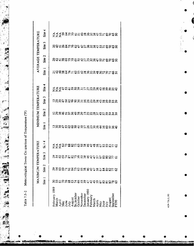
< < a, r i 0 -cn 0 ýoC-4 0 0

* 4P4

4A in %ol Nn 4m m cnk "i

C(7 a i~ oD r- %- 0 'iý 00 (7, kn Wý 00 t- M t- '0 ON - M r,

V2

H

Hcu

0

o P4 ~

C) kn 00 \ -d otNIw-

o PA

Hz H

Table 7.5-3 Meteorological Tower Comparison of Precipitation (inches)

MONTHLY TOTALS

Site I Site 2 Site 3 Site 4

FEB 1989 0.09 0.06 0.20 NA

MAR 0.30 0.03 0.06 NA

APR 0.00 0.00 0.10 NA

MAY 1.47 1.04 3.18 6.71

JUN 0.47 1.00 1.57 2.39

JUL 0.45 0.55 1.23 1.70

AUG 0.47 1.48 0.69 0.90

*SEP 1.05 0.55 1.54 0.02

OCT 0.211 0.27 0.32 0.29

NOV 0.01 0.03 0.03 0.03

*DEC 0.38, 0.21 0.30 0.22

JAN 1990 0.29 0.23 0.26 0;

FEB 0.12 0.13 0.20 0.11

MAR 2.18 1.06 2.68 1.97

APR 0.48 0.40 0.72 0.58

MAY 1.83 0.59 1.56 1.58

JUN 0.28 0.14 0.32 0.00

JUL 2.42 1.34 2.49 2.58

AUG 2.17 1.79 2.81 2.42

SEP 1.18 0.59 1.16 1.18

*FY90OTOTAL 11.55 NA* 12.85 11.28

*Equipment problems during FY90 invalidated these data.

AIR-TBLI.90

fiujW 0>- __

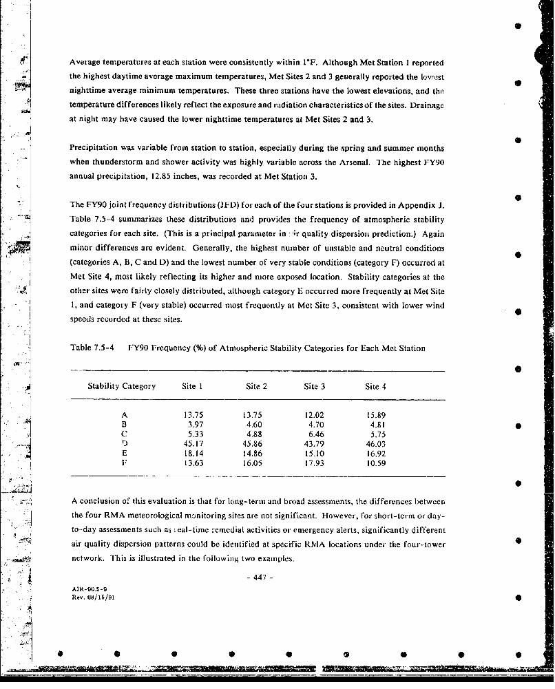
Average temperatures at each station were consistently within I'F. Although Met Station 1 reported

the highest daytime average maximum temperatures, Met Sites 2 and 3 generally reported the lowest

-• nighttime average minimum temperatures. These three stations have the lowest elevations, and the

temperature differences likely reflect the exposure and radiation characteristics of the sites. Drainage

at night may have caused the lower nighttime temperatures at Met Sites 2 and 3.

Precipitation was variable from station to station, especially during the spring and summer months

when thunderstorm and shower activity was highly variable across the Arsenal. The highest FY90

annual precipitation, 12.85 inches, was recorded at Met Station 3.

The FY90 joint frequency distributions (JFD) for each of the four stations is provided in Appendix J,

Table 7.5-4 summarizes these distributions and provides the frequency of atmospheric stability

categories for each site. (This is a principal parameter in :';r quality dispersion prediction.) Again

minor differences are evident, Generally, the highest number of unstable and neutral conditions

(categories A, B, C and D) and the lowest number of very stable conditions (category F) occurred at

Met Site 4, most likely reflecting its higher and more exposed location. Stability categories at the

other sites were fairly closely distributed, although category E occurred more frequently at Met Site

1, and category F (very stable) occurred most frequently at Met Site 3, consistent with lower wind

speeds recorded at these sites.

Table 7.5-4 FY90 Frequency (%) of Atmospheric Stability Categories for Each Met Station

Stability Category Site 1 Site 2 Site 3 Site 4

A 13.75 13.75 12.02 15.89B 3.97 4.60 4.70 4.81C 5.33 4.88 6.46 5.75S45.17 45.86 43.79 46.03E 18.14 14.86 15.10 16.92F 13.63 16.05 17.93 10.59

A conclusion oil this evaluation is that for long-term and broad assessments, the differences between

tmeteorological mmnitoring sites are not significant. However, for short-term or day-

to-day assessments such as :eal-time -emedial activities or emergency alerts, significantly different

air quality dispersion patterns could be identified at specific RMA locations under the four-tower -

,,network. Thisis illustrated in the following two examples.

-447 -

Rev. 08/15/,91.

..: .. ........ •...

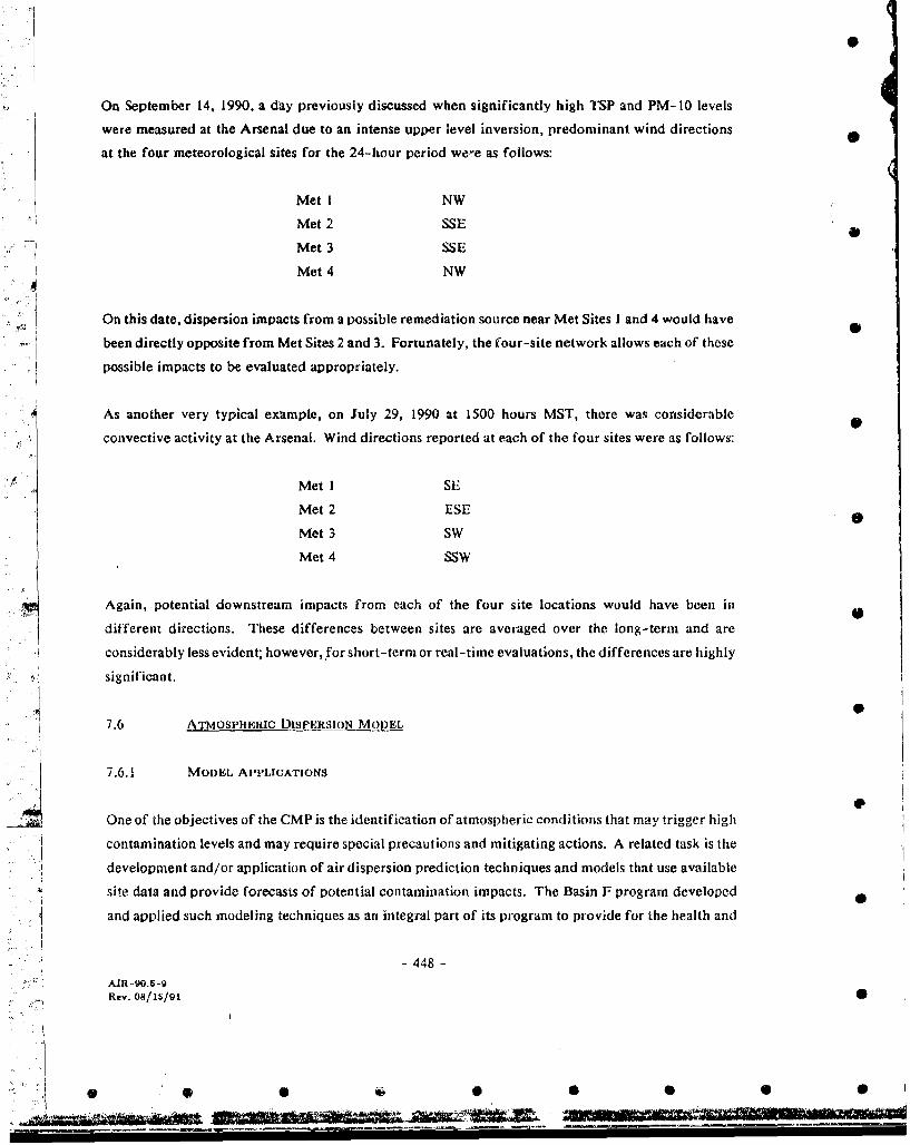
On September 14, 1990, a day previously discussed when significantly high TSP and PM-10 levels

were measured at the Arsenal due to an intense upper level inversion, predominant wind directions

at the four meteorological sites for the 24-hour period we,-e as follows:

Met I NW

Met 2 SSE

Met 3 SSE

Met 4 NW

On this date, dispersion impacts from a possible remediation source near Met Sites I and 4 would have

been directly opposite from Met Sites 2 and 3. Fortunately, the four-site network allows each of these

possible impacts to be evaluated appropriately.

As another very typical example, on July 29, 1990 at 1500 hours MST, there was considerable

convective activity at the Arsenal. Wind directions reported at each of the four sites were as follows:

Met I SE

Met 2 ESE 0

Met 3 SW

Met 4 SSW

Again, potential downstream impacts from each of the four site locations would have been in

different directions. These differences between sites are averaged over the long-term and are

considerably less evident; however, for short-terni or real-time evaluations, the differences are highly

significant.

7.6 ATMOSPHERIC DISPERSION MODEL

7.6.1 MODEL APPLICATIONSI e

One of the objectives of the CMP is the identification of atmospheric conditions that may trigger high

contamination levels and may require special precautions and mitigating actions. A related task is the

"development and/or application of air dispersion prediction techniques and models that use available

site data and provide forecasts of potential contamination impacts. The Basin F program developed

and applied such modeling techniques as an integral part of its program to provide for the health and

-448 -

AIR-90.5-9Rev. 08/16/91 0

i0 0

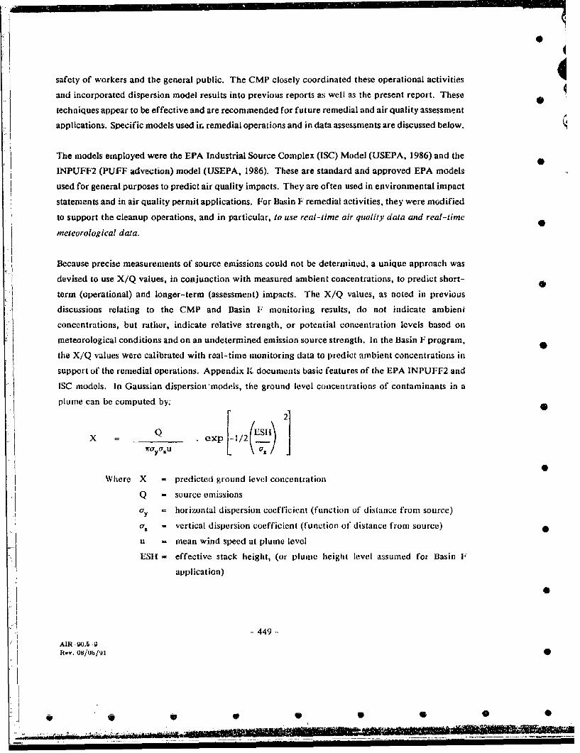
safety of workers and the general public. The CMP closely coordinated these operational activities 4and incorporated dispersion model results into previous reports as well as the present report. These

techniques appear to be effective and are recommended for future remedial and air quality assessment

applications. Specific models used ir, remedial operations and in data assessments are discussed below.

The models employed were the EPA Industrial Source Complex (ISC) Model (USEPA, 1986) and the

INPUFF2 (PUFF advection) model (USEPA, 1986). These are standard and approved EPA models

used for general purposes to predict air quality impacts. They are often used in environmental impact

statements and in air quality permit applications. For Basin F remedial activities, they were modified

to support the cleanup operations, and in particular, to use real-time air quality data and real-time

meteorological data.

Because precise measurements of source emissions could not be determined, a unique approach was

devised to use X/Q values, in conjunction with measured ambient concentrations, to predict short-

term (operational) and longer-term (assessment) impacts. The X/Q values, as rioted in previous

discussions relating to the CMP and Basin F monitoring results, do not indicate ambient

concentrations, but rather, indicate relative strength, or potential concentration levels based on

meteorological conditions and on an undetermined emission source strength. In the Basin F program,

the X/Q values were calibrated with real-time monitoring data to predict ambient concentrations in

support of the remedial operations. Appendix K documents basic features of the EPA INPUFF2 and

ISC models. In Gaussian dispersion models, the ground level concentrations of contaminants in a

plume can be computed by:

21x oexp-.1/2

Xcr7Ou-- --.\=/]

o

Where X - predicted ground level concentration

Q - source emissions

cry = horizontal dispersion coefficient (function of distance from source)

a. - vertical dispersion coefficient (function of distance from source)

u = mean wind speed at plume level

ESH - effective stack height, (or plume height level assumed for Basin F

application)

- 449 -AIR--90.5 -9Rev. 08/06/91

S46-'.. *

When the source emission term is not determined, the equation can be written as follows:

rayo~u a.\%0

For the present assessment applications, assuming that Q is constant, or near constant (at any given

time), the relationship between an observed (monitored) concentration at a specific grid location

where a X/Q was calculated, and at another unmonitored location where a X/Q was also determined

was the ratio between the two values. This was a very simple approach, but was highly effective in

determining the spread of a dispersion plume beyond and between the monitoring networks. The

technique will allow for the prediction of future concentrations during ongoing operations, assuming

that emissions do not significantly change during a particular operation. As remedial progress

continues and emissions are eventually reduced, observed concentrations for a specified X/Q should

also be reduced. This was the case for the IRA-F data for Phase 4 provided in this report, as

compared to Phase I results discussed in the FY88 Data Assessment Report. Thus, the model has the

potential to evaluate remedial progress under comparable meteorological and air dispersion conditions.

The PUFF model was used primarily for short-term predictions at Basin F in conjunction with real-

time operations. Air monitoring was conducted using HNU, OVA, ammonia and dust monitors at

various remedial activity areas and along the Exclusion Zone perimeter. Perimeter readings were

taken at four fixed locations and also downstream from Basin F, based on the prevailing wind, where

max; ,um concentrations were anticipated. Concurrent with each monitoring reading, the PUFF

model was run to determine the trajectory of the contamination plume. The X/Q values of the model

were then immediately matched with actual monitored data to determine the potential distribution

of the plume trajectory and the likelihood of Level B exceedances outside the protected areas. A

maximum limit of I ppm was established for expansion of the Exclusion Zone and/or evacuation of

personnel without protective clothing and equipment.

Both the PUFF model and the ISC model have the capability to provide longer-term X/Q dispersion

assessments. Because the PUFF model operates on 15-minute trajectories, it takes much longer to

run, and the ISC model was primarily employed for 24-hour assessments and beyond. However, the

PUFF model can be used to assess longer-term episodes if more refined or sensitive analyses are

required.

450 -

AIR-90.b-9Re~v. 08/O5/91S

'66. .." . . . .., ....; ..

0 -

The results of the CMP and Basin F monitoring programs, discussed in Section 4, were compared with

dispersion analyses obtained from the EPA Industrial Source Complex model. As noted, these

evaluations provided highly useful information for associating dispersion patterns and meteorological

conditions with observed and potential air contamination levels. When a distinct source was evident,

such as Basin F, Basin A, or the South Plants, the model identified tho spread of the dispersion plume

downstream from the source. The concurrent monitored data then provided a mechanism for

calibrating and projecting ambient concentrations throughout the Arsenal and beyond its boundaries.

The model identified worst-case meteorological conditions and seasonal and diurnal effects, thus

providing a basis for mitigation actions. For future assessments, it provides a basis for evaluating

remedial progress by ensuring that monitoring results are compared to similar worst-case meteorology

and seasonal conditions.

The effectiveness of model applications is evident from the data and comparisons shown in the

proceeding sections. The impacts from known RMA sources, or remedial activities, have been

identified and the relative strength of these impacts with distance from the source have been

t, quantitatively determined. There is also considerable scatter of X/Q values at specific site locations,

which can be attributed to many factors beyond the simplified mnodel's present capabilities. These

include variations in source emissions and remedial production activity, both of which obviously

result in variations in concentration levels downwind from the source; the existence of other potential

area and local sources, which present a "noise" factor in the database; short-term meteorologicalS influences that -ire not irntegrated into the hourly Industrial Source Complex database (this suggests

the special advantage in using the short-term PUFF trajectories); and the general complexity of the

dispersion process that is not entirely identified in the model.

In summary, the PUFF and Industrial Source Complex models, using the X/Q calibration approach,

were and will continue to be workable vehicles for projecting contamination levels during remedial

activities and for assessing remedial progress. It is not the purpose of the CMP to do extensive

research investigations to improve model validation and appliations. Nevertheless several practical

follow-on efforts may be applied in future CMP evaluations that would not only improve the models

but would also provide considerable insight into the general assessment of RMA contamination levels 0during subsequent remedial activities. These are discussed below.

AO

-451-AIR -90.5-9Rw 06/15/91

•) 0. 4 0 0 WS)•

S... : . ... ;' I I I I I I I I 11

7.6.2 ADDITIONAL MODEL APPROACHES AND ANALYSES

S.7.6.2.1 Source Emissions Characterization

The standard dispersion model predicts ambient concentrations based upon meteorological factors and

a known, or estimated, emission source. The Basin F real-time application, as well as for the CMP,

have to a certain extent effectively bypassed the emissions term and substituted a mechanism (X/Q

values) for providing contamination level- based upon concurrent monitoring data. More precise data

on emission releases at potential RMA and off-Arsenal con*amination sources will add an additional

dimension to the modeling and prediction capabilities. Data indicating the combination of emission

levels, meteorological factors and resultant ambient concentrations will also allow for still further

refinements of the model. For subsequent cleanup activities at RMA requiring air quality impact

assessments, precise emissions data and characterizations will cnhance prediction capabilities.

407.6.2.2 Remedial Activity Production Data

It is evident from the Basin F monitoring results during remedial operations and frtom the previous

Remedial Investigation Program results prior to remedial operations that the cleanup activities resulted

in increases in some of the monitored pollutants, in particular TSP, pesticides, organic compounds and

some metals. It may be assumed that these increases were a direct consequence of and proportional

to the extent of remedial efforts on a day-to-day basis. Various information pertaining to the status

and intensity of cleanup operations, including the tons of soil and sludge ruinoved and hauled each

day, the type and number of vehicles and type of equipment employed, storage areas and uncovered

waste pile areas, the number of gallor.s of liquid transported, and any othei emission-producing

factors related to operations would be especially useful in assessing relative emris!:ions potential and

in refining model prediction capabilities. These data were available, to a limited extent, during the

Basin F operations, but not necessarily on a real-time basis; this made it difficult to interpret the

cause of higher contamination events and the extent of mitigation efforts that were needed. It should

be noted that many industrial real-time air quality prediction systems are directly related to

production factors (Edson, 1976, 1977, 1978), and this approach would have equally valid application

for waste cleanup operations.

- 452 -

AIR-eO.869Rey. 08/16/91

0 .

-i" D••• *@ @ (±

7.6.2.3 Local gnd Regional Emissions Inventory

One of the difficulties in analyzing the CMP and Basin F data was that there were obviously other

local and regional air emissions sources in the RMA vicinity that contributed to air pollution levels

measured at RMA monitoring sites. As noted in the data evaluations, metropolitan Denver was a

source of TSP, PM- 10, some metals, gaseous criteria pollutants and, undoubtedly, certain organics.

Also, various industrial sources and farming areas in North Denver, Commerce City and Adams

County may have contributed to organics and other potential contaminants. In this report, an attempt

has been made to identify these sources in order to properly evaluate their contribution to RMA

monitored data. They present an unknown (or noise) factor in the dispersion model prediction

evaluations of potential RMA contamination and remedial impacts unless properly identified.

Consequently, an inventory of local off-RMA sources is highly desirable for the interpretation of

baseline data and remedial progress at RMA. Work has begun on this effort and an inventory of

known sources is included in this report; these data contribute to the overall analyses. Additional

work is also required in identifying the contributions and impacts of metropolitan mobile sources on

RMA monitoring results. Quantification of such influences would again enhance model evaluations

and prediction capabilities. Much of this information is available in the Colorado Department of

Health files, the Air Toxics Study for Denver conducted by EPA and other reports including the

Citizens Report on Toxic Pollution in Colorado (see Section 4.0).

7.6.2.4 imirical/Statistical Adiustments

A final approach for model improvement is the application of empirical techniques and pertinent, or

unique, physical relationships to improve model capabilities. As examples, it is generally agreed that

organics are released into the atmosphere at warmer temperatures and also under certain favorable

air pressur. conditions; TSP, metals, and PM- 10 are generally higher after certain threshold wind gust

levels are achieved. Also, very localized, topographic site-specific characteristics may be evident in

the spread of potential air contaminants over the area which are not considered in the dispersion

inodel. The database now being collected provides a mechanism for establishing some of these

influences; some have already been identified in the present report. It is anticipated that this effort

will continue, and if possible, validated relationships will be incorporated into model apl.ications.

0

- 453 -

"Rev. 08/15/91

.4 ,:•

, 0 0 0

'a7~

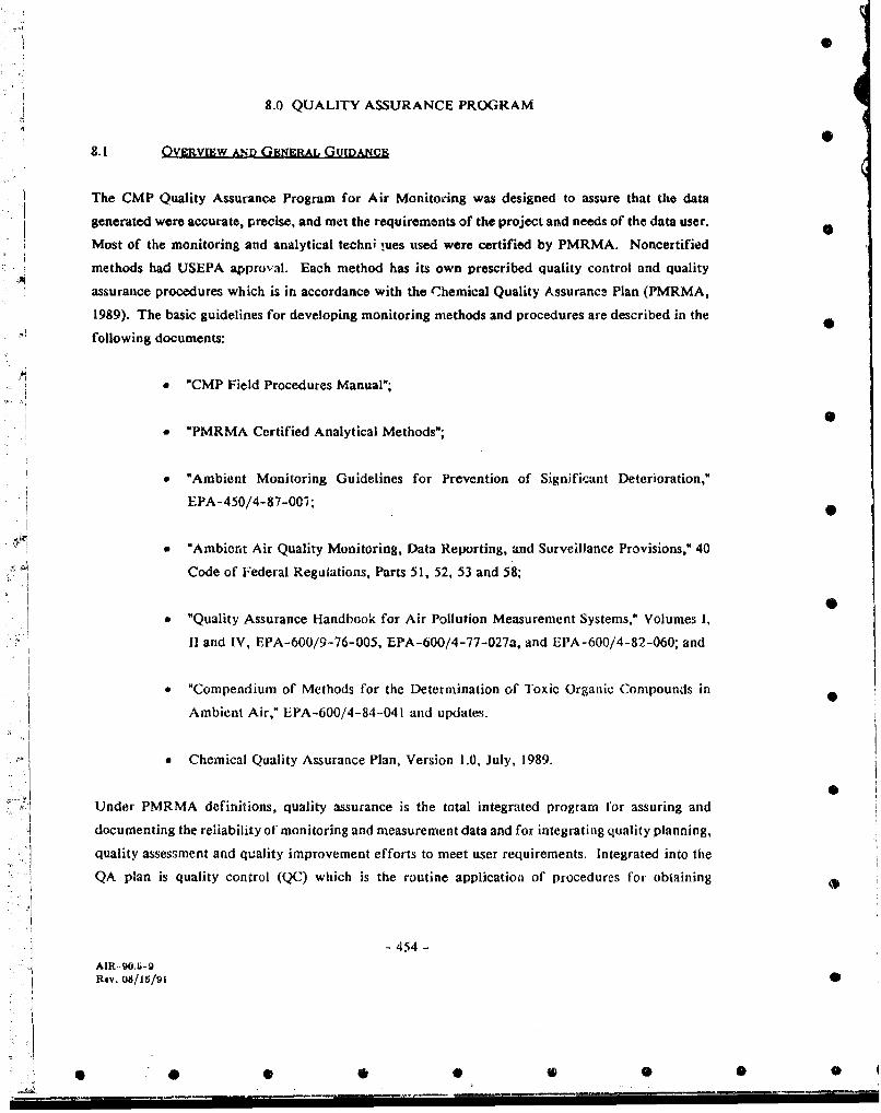
0

8.0 QUALITY ASSURANCE PROGRAM

8.1 OVERVIEW AND GENERAL GuIDANCE

The CMP Quality Assurance Program for Air Monitoring was designed to assure that the data

generated were accurate, precise, and met the requirements of the project and needs of the data user.

Most of the monitoring and analytical techni -.ues used were certified by PMRMA. Noncertified

methods had USEPA approval. Each method has its own prescribed quality control and quality

assurance procedures which is in accordance with the Chemical Quality Assurancz Plan (PMRMA,

1989). The basic guidelines for developing monitoring methods and procedures are described in the 0

following documents:

"CMP Field Procedures Manual";

0"PMRMA Certified Analytical Methods";

"* "Ambient Monitoring Guidelines for Prevention of Significant Deterioration,"

EPA-450/4-87-00i;

"* "Ambient Air Quality Monitoring, Data Reporting, and Surveillance Provisions," 40

Code of Federal Regulations, Parts 51, 52, 53 and 58;t0

"* "Quality Assurance Handbook for Air Pollution Measurement Systems," Volumes I,

II and IV, EPA-600/9-76-005, EPA-600/4-77-027a, and EPA-600/4-82-060; and

"* "Compendium of Methods for the Determination of Toxic Organic Compounds in

Ambient Air," EPA-600/4-84-041 and updates.

* Chemical Quality Assurance Plan, Version 1.0, July, 1989.

Under PMRMA definitions, quality assurance is the total integrated program for assuring and

documenting the reliability of monitoring and measurement data and for integrating quality planning,

quality assessment and quality improvement efforts to meet user requirements. Integrated into the

QA plan is quality control (QC) which is the routine application of procedures for obtaining

-454 -" 4 AIR-90.ii-9

Rev. 08/15/91 •

S " 0•0 0 0 0 0

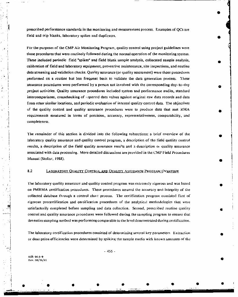
prescribed performance standards in the monitoring and measurement process. Examples of QCs are

field and trip blanks, laboratory spikes and duplicates.

For the purposes of the CMP Air Monitoring Program, quality control using project guidelines were

those procedures that were routinely followed during the normal operation of the monitoring system.

These included periodic field "spikes" and field blank sample analysis, collocated sample analysis,

calibration of field and laboratory equipment, preventive maintenance, site inspections, and routine

data screening and validation checks. Quality assurance (or quality assessment) were those procedures

performed on a routine but less frequent basis to validate the data generation process. These

assurance procedures were performed by a person not involved with the corresponding day-to-day 0

project activities. Quality assurance procedures included system and performance audits, standard

intercomparisons, crosschecking of c cported data values against original raw data records and data

from other similar locations, and periodic evaluation of internal quality control data. The objectives

of' the quality control and quality assurance procedures were to produce data that met RMA

requirements measured in terms of precision, accuracy, representativeness, comparability, and

* "completeness.

The remainder of this section is divided into tile following subsections: a brief overview of' the

laboratory quality assurance and quality control program, a description of the field quality control

results, a description of the field quality assurance results and a description oe quality assurance

associated with data processing. More detailed discussions are provided in the CMNi Field Procedures

Manual (Stollar, 1988). •

8.2 LABORATORY QUALITY CONTROL AND OuALivTY AsIs.NcE PrQ M I.)VFJtVjN.W

The laboratory quality assurance and quality control program was extremely rigorous and was based 0

on PMRMA certification procedures. These procedures assured the accuracy and integrity of the

collected database through a control chali I process. The certification program consisted first of

rigorous precertification and certification procedures of the analytical methodologies that were

satisfactorily completed before sampling and data collection. Second, prescribed routine quality

control and quality assurance procedures were followed during the sampling program to ensure that

the entire sampling method was performing comparable to the level demonstrated during certification.

The laboratory certification procedures consisted of determining several key parameters. Extraction

or desoi-ption efficiencies were determined by spiking the sample media with known amounts of the

. 455AtMR- 9g1.5-9

ReV. 08/iG/9l D

0 5 5 5 5 5 0 0 Q0• -. =d . . . . . . . .. .. . .. .. . ,... ... . ' _-• . . • ._ _ _.. . . - .- -

SI. target analytes and performing the analyses along the analytical guidelines. A percent recovery for

each of the compounds was determined from multiple piking tests. Accuracy adjustments were

determined from the mean of the percent recoveries at certification. One and two standard deviations

from the mean of the recovery data was used to validate tbh subsequent data giving a 95 percent

confidence level to the data. A range of concentrations was used to test the linearity of the laboratory

instrument response and to certify an analytical range for each target analyte, with values denoted

as the upper and lower certified reporting limits.

Reporting ranges were determined at the time of certification. Values found below this range were

reported as "less than" the lower reporting limit. Values found above this range were reported as

" greater than" (GT), and were then estimated. These values are considered qualitative, and are used

as a "best guess" of concentration ranges. Upper limits did not apply to TSP and PM-10

measurements. For SVOCs and metals analysis, extract solutions were diluted (if possible) for

reanalysis if the initial readings were above the certified range and holding times for the extracts had

not yet expired.

The VOC laboratory analysis technique differed significantly from other techniques because there

was no possibility of diluting or reanalyzing samples. The VOC Tenax sorption tube was placed into

a heating block connected to the inlet of' the analytical instrument. This block or thermal desorber

was quickly heated to desorb all the volatile compounds off of the Tenax. A small air flow was passed

through the tube simultaneously, which allowed these compounds to be quickly injected into the

analytical instrument through a heated stainless-steel interface. Therefore, this method was a "one

shot" technique, and if the sample concentration was outside certified limits, there was no way to

dilute and reanflyze the sample. In the I'Y90 program, there were instances where a sample had

collected an amount above the certified range for some compounds. An assessment of the

concentration was made by using the hypothesized concentration curve above the certified range.

Such results represented the best estimate of the observed concentrations; however, these data were

not certified in accordance with I1MKMA standards and were likely to represent a low estimate of

actual concentrations.

aTle above measures of laboratory accuracies, certified ranges, and extraction efficiencies weredirectly incorporated into the database processing system that was used to report air quality data. Th is

system is the Installation Restoration Data Management System (IRDMS). In Ii(l)MS, the raw

laboratory results are sent to Ebasco, the data are checked for errors, adjusted for flow volumes, and

sent to DP Associates and held in the QC holding database. Once the Army has accepted the data as

': : - 456 -

Alit .90.5 )

Rev. 08/15/91 5

S 6 5 S • • S 0 • •S... .. . ..... - - i .... . - i- -

meeting the QA criteria, it is then corrected for accuracy and loaded into the official database. Data

outside of certified ranges and rejected under the QA criteria are placed in a rejected data file for

informational use only. 1 'ie resulting product is a high-quality analytical database that was available

to field personnel for calculating ambient concentration data.

8.3 faLD QUALITY Ol 1110iTR PRORAM •

8.3.1 ORGANIZATION

The field inoniturirng team was organized to conduct several activities that provided data quality

control for the program. At the outset, a monitoring team supervisor was designated and a set of

procedures was drawn up to address quality control. The field supervisor and project manager

insured that the quality control procedures were implemented.

Standard field data sheets were used by the project team. Each team member was trained in the use

and entry of data on this form. Forms were documented in project files, and copies were distributed

to the project manager for periodic review. Calibration data sheets were also drawn up for the

project and the calibration team was trained in their use. The field and calibration data sheets were

stored on-site and a copy was sent to the project manager. The field supervisor was responsible for

ensuring that these records were maintained, routinely reviewed and updated, and used by the data

processing personnel. Final deposition of these documents are the project files and will ultimately

be sent to PMRMA at project close-out.

8.3.2 FIELD PROGRAM QUALITY CONTROL

For each of the sampling techniques used, the air quality technical plan specifies target flow rates and

sampling durations. These values were used during the field sampling activities and were documented

by periodic equipment calibrations as well as checks during each sampling event. Quality assurance

* limits were set up using the EPA Quality Assurance llandbooks for acceptable instrument

performance. Whenever a flow rate or elapsed tinier was outside of acceptable limits, corrective

maintenance was performed to bring the defective component or activity back into tolerance. The

activities were documented and kept with field file records.

The high-volume field equipment used to sample TSP, PM- 10 and metals was electronically Hlow-

controlled to maintain a constant flow rate. A certified flow measuring orifice was routinely used

457 -

AI Rw.,f.il .9S.. .. • liy. u8/11iq91

0

to calibrate the flow rate set point. Calibrations were performed once per quarter or more frequently

if needed. For the SVOC and OCP high-volume samplers, a flow rate gauge was u5-d to monitor the

flow rate of the sampler. During calibration of these samplers, a range of flow rates was measured

with the orifice, and a linear regression was developed relating the sample indicator reading to the

orifice flow rate. The maximum deviation of any flow rate point from the linearly interpolated value

should be less than 7 percent for the TSP, PM-10, SVOC, and OCP samplers. For TSP and PM-10,visual inspection of the Dixon chart indicated whether the flow deviated during the sampling period.

The low-volume field sampling equipment, which measured VOCs, mercury and ammonia, were

Gilian constant flow sampling pumps equipped with rotameters. Before each field sampling event

the pumps were calibrated and set to specific flow rates as determined by a certified masF flowmeter.

During a sampling event, personnel routinely inspected the rotameter to ensure correct flow rate

readings.

8.3.3 QUALITY CONTROL FIELD SAMPLE RLSULTS

8.3.3.1 VOC Ouality Control Rjl.9_!.i

The specified requirement for determining efficiency of the sampling equipment is to compare the

volume of air sampled to establish acceptable sampling volumes. The Tenax collector for, VOC

sampling will not capture all of a particular compound greater than a specified sample volume. The

sampling volume should not exceed the established "breakthrough" volume for the compound of

interest in relation to the amount of sampling matrix (i.e., Tenax).

The sampling media employed consists of a front sorbent tube containing Tenax and a second or

backup tube containing Tenax and charcoal. The tubes were analyzed simultaneously, therefore,

actual "breakthrough" ' is not assessed. Theoretical "breakthrough" volumes were calculated based

on the amount of Tenax contained in the tubes.

The standard VOC method prescribes the use of collocated samples as a quality assurance procedure

that can be used to increase confidence in the data that are generated. This techniq.ue has been used

by the CMP and results are discussed in Section 8.4. The recommended performance criteria is that

the mean difference between the pairs of collocated samples should generally be within 25 percent

*• of the sample mean.

S•i -4.58 -

*AIRI- 9¢d.5i-

Rev. fI8/I/91 S

* 2 e -

Field blank values were also compared to field sample analytical values. As stated in the VOC

X ",,method, the blank sorbent trap should cL -tin less than 10 ng of the target compounds before it is

sent to the field. Table 8.3-1 presents a summary of the target VOC blank values for all of the field 0

and trip blanks during FY90. For most of the target compounds, field blank levels were less than the

certified reporting limit (which generally corresponds to approximately 10 ng per sample). However,

some field blanký 'wed detectable levels of benzene, methylene chloride, and I J, l-trichloroethane

(I ITCE). Jienzeae was detected in all field blanks except one, and five samples had methylene 0

chorride levels above the certified reporting limit. The level of 11 ITCE detected was near the lower

certfied reporting limit. Therefore, because blank correction was not performed during the CMP

on VOC data, the beozene ad methylene chloride data especially should be considered coaservative,

and the actual ambient concentrations may be lower than presented in this report. Detections of 0

benzene in the blanks car) be explained by Walling et aL. (1986), who observed a decomposition

product of benzene whe a Tenax was repeatedly heated to 200"C. The other two are common

laboratory solvents and are easily retained on Tenax.0

3.3.3.2 Se.V Clatile Oryanics and O_.anics on PUF Qalitv Control Results

Quality controJ samples ,or semi-volatile organic compounds and organochlorine pesticides consisted

of field blanks, trip blanks and z,er.ted field spikes. The SVOC and OCP sampling methods were 0

identical; both consisted of a polyurethane foam sorbent plug and quartz filter used i, high--volume

sampler. In the SVOC analytical method, gas chroinatograph/mass spectrometer (GC/MS), was used

for detection. This analytical device has the ability to measure a wide variety of compounds, other

than the target analytes, yet has a moderately high detection limit. For OCP samples, a gas 0

chromatograph/electron capture detector (GC/ECD) was used. This device analyzed only the

crganochlorine pesticides for which it was certified and had a very low detection limit. All

01 t.,anochlorine pesticidcs, with the exception o' aldrin, were iacluded in the SVOC target list. The

aldrin concentrations repo:ted for the Or'P technique must be used with caution. In actual field

sampling there is the pu .;ial for stripping or oxilation of aldrin, and the recovery of spiked aldrin

samples is known to be low (USEPA, 1984).

Two field spiking events were perfornied for CMP's 1990 Air Monitoring program. The results For S

the first (SVC,') effort are listed in Table 8.3-2. The spiking solution was prepared by the

ESE/Denver laboratory and sent to the field team.

459. - 0 }. 9- 1

h~ey. 08/15/l91

0t

S" S •., u, • luw,, ,=t*,••, *•,• 0. ,S ,.i, 0 ,•••-• .,, ,bs*g•;•.

- - - - - --

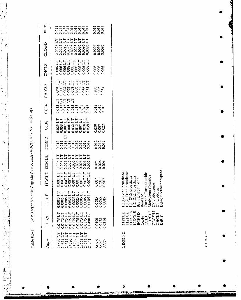
~ O O 00 000C >C)C >ýo C )C

CU 00 000000CC C 000-6 00 0 5* 0 000 ; ;

1 w0 00 W00 0 -0oc0 C 000-

C) C 0 000 00 0C)C lC40 0

C ----- h--- -

1 Q

Cý 00 000? 000 C ýq

V~~~C 0CO000 0w 00000 O00 00 o00

00~~Clr C C R qqC0 00 00 000 )C)C >C C .C pu uuc

Cd kHr ~~~ ~ Z 000000

wllll w n W V e4CIbk^C'J cC> nCD

0 '- ... .00 0000 0 00

- 0 00 0 0 0

ol co )CACo CAJ F-FHFH -j

A) - 4-

In.2w n I n In L l )ý l0 CDC) o C>C> > C)czý C) Cl S

14C ! lc !C0 C> C) C>C )V ) > C 0C

00 00 00 0001% V)k 41 ýin % nI-u 00 0 0 0 000 ----

> ý 00 00 00 000 5ýqqqqC ýQ C nC5(DH >H=HH >C

InW)%nk V -) l -knin-- lk^I

c-:,6 :) C.) I> c CDO C)

00000000 00 wwo 0fJ 0000> 000 ) )C)CDC Z ZH C>0C0(D0000C>0 000>CýC

H~-~ HHHc)

Ink U nk nWýV ) t l l(' \ O0N hO Na NON0 NC\Ocu 6c6665d

U ~ C qC) C>0 0 ) 0 D C)C> C

< HH 4 HHHHHw)I n w )%n4l )kýI

cD C>C C )cDC !) > DC

q C: 000 qC ý ý CýC<D C-1o c oo 000 C C ý DC

IC HH HH Hcn m000m l f n11

00000000. 00C> (D o~ o o 000>C>C ý ýC C ý

Ind c 000 InL n -w W nI 0146 , .

'f~r- r- rc <- -- o

Wt X -.- , o---.-r:F- FH F-HHF l

C l ~ l ~ ~ lri lri, Q

0 Inwl n w~ InIn ý w, l0

In m l m m In "I0

Table 8.3-2 Summary of Semi-Volatile Organic Compounds Results of Field Spiking4

Target Analyte Control Conc. (pug) % of Recovery# #I % of Recovery #2

Aidrin LT* LT LT*Atrazine LT 39 32*Chlordane LT 110 102

CPMS LT LT LTCPMSO LT 42 93CPMS02 LT 65 81DBCP LT LT LTE)CPD LT LT LTDDVP LT LT LTDIM? LT LT LTDITH LT LT LTIildi LT 149 129 0

DMXP LT LT LTEndrin LT 160 138HCBD LT LT LTIsodrin LT LT LTMalathion LT 80 61Oxathiane LT LT LT'PPDDE LT 150 123PPDDT LT 135 125Parathion LT 103 81Supona LT' 153 91

Note: 45 ag were spiked onto 2 separate PUFS.

*LT <,fers vo detections less than the lower certified reporting limit. Recoveries are generallyless than 10%.

AIR-T)IL1 qf)

----- --- 0

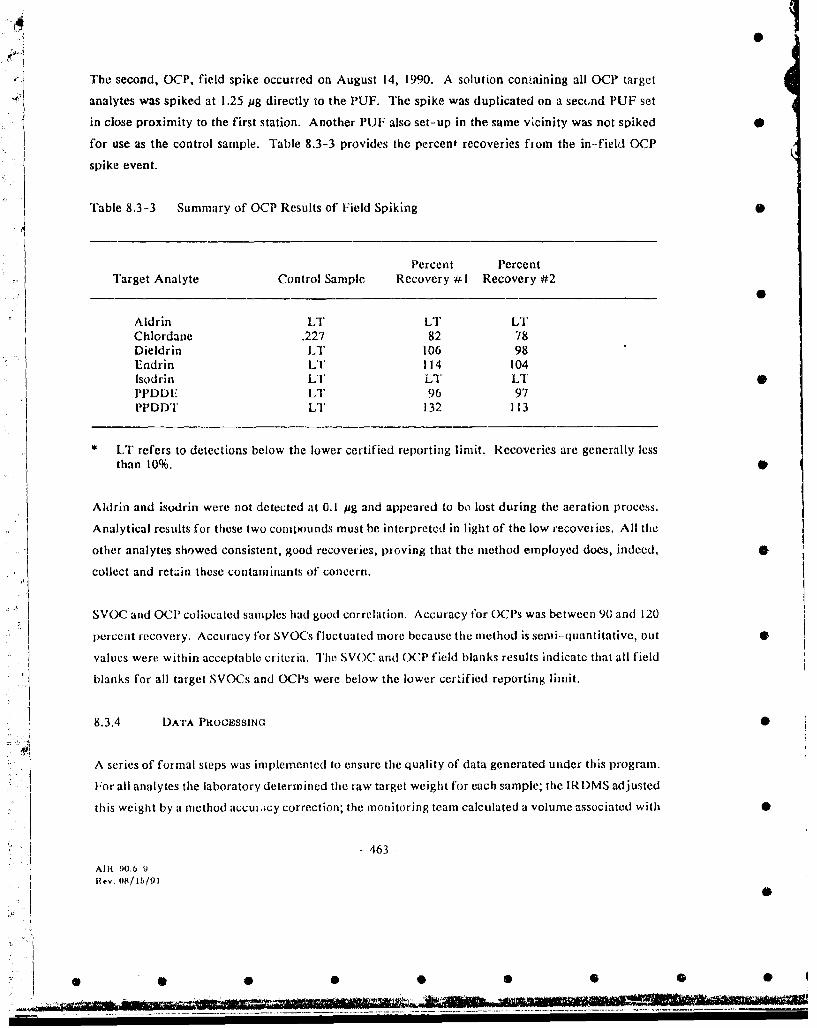
4@

The second, OCP, field spike occurred on August 14, 1990. A solution containing all OCP target

analytes was spiked at 1.25 ug directly to the PUF. The spike was duplicated on a secnd PUF set

in close proximity to the first station. Another PUF also set-up in the same vicinity was not spiked

for use as the control sample. Table 8.3-3 provides the percent recoveries from the in-field ()CP

spike event.

Table 8.3-3 Summary of OCP Results of Field Spiking 0

Percent PercentTarget Analyte Control Sample Recovery #1 Recovery #2

Aldrin LT L]T LTChlordane .227 82 78Dieldrin Li 106 98Endrin LT 114 104Isodrin LT LT LT 0PPDDE LT 96 97PPDDT LT 132 113

• LT refers to detections below the lower certified reporting limit. Recoveries are generally less

than 10%. 0

Aldrin and isodrin were not detected at 0.1 pg and appeared to bo. lost during the aeration process.

Analytical results for these two compounds must be interpreted in light of the low recoveries. All the

other analytes showed consistent, good recoveries, proving that the method employed does, indeed, 0

collect and retuin these contaminants of concern.

SVOC and OCP collocated samples had good correlation. Accuracy for OCAPs was between 90 and 120

percent recovery. Accuracy for SVOCs fluctuated more because the method is semi-quantitative, out 0

values were within acceptable criteria. The SVOC and OCP field blanks results indicate that all field

blanks for all target SVOCs and OCl's were below the lower certified reporting limit.

8.3.4 DATA PROCESSING

A series of formal steps was implemented to ensure the quality of data generated under this program.

* For all analytes the laboratory determined the raw target weight for each sample; the IRDMS adjusted

this weight by a method accui .cy correction; the monitoring team calculated a volume associated with •

463

Alit 90.5 9)Re•v. 08/16/91

..................... .....................

S

each sample; and the adjusted weight was divided by the sample volume to obtain a concentration per

unit volume of air sampled.

The quality assurance group reviewed the laboratory quality control data, including surrogate and

spiked recoveries and general compliance with the PMRMA quality control methodology. The

acceptability of each lot was addressed by the laboratory and was reviewed for approval by the quality

assurance team. The control charts were reviewed to 'indicate method control and submitted to

PMRMA. The laboratory provided a paper copy and a diskette of uncorrected sample weights to the

data management group. The printout of diskette data was compared with the papercopy results and

any discrepancies were resolved. For each target compound in each group of data, a check was made

of at least one sample to assess the method accuracy correction.

The field team generated a sample volume computation on spreadsheet software using the field

calibration, flow check and timing data. Spreadsheet entries were checked and volume computations

were verified by the quality assurance group. The data processing group generated sample

concentrations from the weight and volume data. A series of group checks and record checks verified

the conduct of the quality control effort, holding times, and that data were within certified limits.

Finally, the quality assurance program provided documentation that the database was generated in

accordance with quality assurance procedures.

8.4 ASSESSMENT 01 DATA PRECISION AND COLLOCATED DUPI!CATE SAMPLINO RESULTS

The CMP collocated sampling effort was performed at Site AQ5, and the pairs of samplers were

located approximately 3 meters from one another. Results were calculated '.'or all target compounds

* iand detailed data are presented in Appendix It. Collocated sample comparisons are listed in Table

8.4-1. Only the sample pairs with results above the lower certified reporting limit (LCRL) were used

to compare collocated results. The average percent difference is the mean. difference as a percent of 0

the mean collocated sample concentrations. For TSP, PM- 10, and metals a pair of collocated samples

was taken for every collection date set at every 6 days and for every high event episode; therefore,

65 sets of comparable data for collocated metals samples exist for the 1990 monitoring year under

CMP. For TSP and PM-10 the ±95 percent confidence intervals were computed and expressed as a

percent of sample mean. For TSP, these intervals range from -10.2 percent ;o 8.0 percent. For PM-

10, the range is -23.3 percent to 18.3 percent.

0

- 464 -

AMIR-90.5-9Rev. 08/1/91

:4, : • U

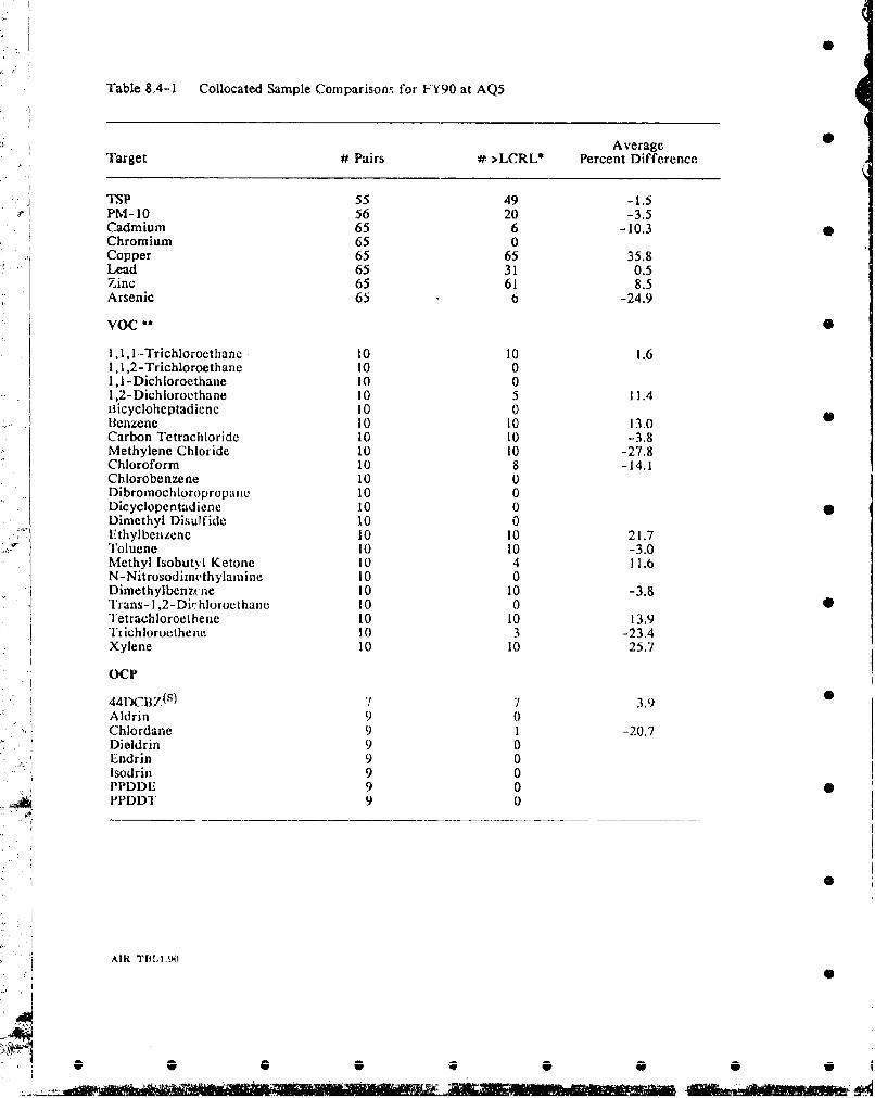
Table 8,4-1 Collocated Sample Comparisons for FY90 at AQ5

/S

AverageTarget # Pairs # >LCRL* Percent Difference

TSP 55 49 -1.5PM-10 56 20 -3.5Cadmium 65 6 -10.3 0Chromium 65 0Copper 65 65 35.8Lead 65 31 0.5Zinc 65 61 8.5Arsenic 65 6 -24.9

VOCb* 0

1,1, 1.-Trichloroetliane 10 10 1.61,1,2-Trichloroethane 10 01,1-Dichloroethane 10 01,2-Dichloroethane 10 5 11.4i3icycloheptadiene 10 0Benzene 10 10 13.0Carbon Tetrachloride 10 10 -3.8Methylene Chloride 10 10 -27.8Chloroform 10 8 -14.1Chlorobenzene 10 0Dibromochloropropane 10 0Dicyclopentadiene 10 0 0Dimethyl Disulfide 10 0Ethylbenzene 10 10 21.7Toluene 10 10 -3.0Methyl lsobutxl Ketone 10 4 11.6N-Nitrosodimethylainine 10 0Dimethylbenzcne 10 10 -3.8Trans- 1,2-Dichloroethane 10 0 5Tetrachloroethene 10 10 13.9Trichloroethene 10 3 -23.4Xylene 10 10 25.7

S~OCP

44DC1BZ(5 ) 7" 7 3.9Aldrin 9 0Chlordane 9 I -20.7Dieldrin 9 0Endrin 9 0Isodrin 9 0PPDDE 9 0 0I'PDDT 9 0

AIR TBIII,.940

w 'W-W.0

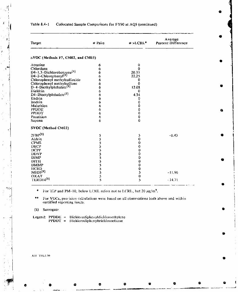
4Table 8.4-1 Collocated Sample Comparisons for FY90 at AQ5 (continued)

AverageTarget 4 Pairs #>LCRL* Percent Difference

z~VO-C (Methods F7, CM02, and CMO3)

Atrazine 6 0Chlordane 6 0D34-1,3-Dichlorobeilzene(s) 6 20.33D34-2-Chlorophenyl s) 6 22,25Chlorophenyl methylsulfoxide60Chlorophenyl methyls 1one 6 0D3-4-D3iethyiphthalatc ST 6 12.08Dieldrin 6 0D4-Dioctylphthalate(S) 6 4.34Endrin 6 0Isodrin 6 0Malathion 6 0PlIIDDE 6 0PPDYI' 6 0Parathion 60Supona 6 0

SVOC (Method CMO3)

21--iP(3) 5 5-.3Aldrin 5 0DlCPM 5 0DCPS 5 0DC1111 5 0DDVP 5 0L)IMP 5 0DITI 1 5 0DMMP 5 0IICI3D 5 0NIID5(3) 5 5 -11.96OXAT 5 0TERI)14(8) 5-1.7

*For 'I1.1 and PM-. 10, below I.CRl. refer riot to 1,CRIZ, hut 20 jig/nmI.

**For VoX~s, precision ca:culatioiis were based on all observations both above and withincertified reporting I iiits.

(S) Surrogate

.1Legend: PPDDE =Dichlorodip~iicuiyldichiloroethiylcne

PPI)DT - 1)iclhlorod iphienyltrichiloroethancii

AM TBLI.Q

UQ

The percent differences were calculated by dividing the difference between the pair by their average.

Percent differences were calculated for positive target analyte values that were PMRMA validated.

Most of the comparisons consistently fell within ±50 percent difference. A few outliers existed for

zinc and copper, which are known contaminants within the glass fiber filter employed by MRI

laboratory and the quartz filter employed by ESE laboratory. One outlier existed for arsenic during

the November 6, 1990 sampling event.

0Generally, the values obtained in comparing collocated samples were within acceptable limits,

indicating that the method was stable and provided comparable results.

Flor TSP and PM-10, the 95 percent confidence limits were calculated on the basis of standard

statistical techniques for normal distributions. These values represent, with 95 percent confidence,

the limits between which the actual median value lies. The observed 95 percent L ,ifidence limits for

total suspended particulates and inhalable particulates all fell within the ±25 percent guideline. The

95 percent confidence limits for lead fell within ±30 percent precision range.

Collocated samples for volatile analysis are also listed in Table 8.4-1. These samples were collected

on high event days as described in Section 4.6, There were 10 sets of collocated samples for the 1990

CMlI Air Monitoring year. All samples were collected at Site AQ5 except for the samples collected

on September 11, 1990 at Site AQI0. Sampling units were spaced in close proximity at approximately

3 ft apart.

Comparisons between the collocated samples are expressed as an average percent difference of all

collocated samples. The volatile sample comn parisons are unique in that many of the target compound

detections are values above the linear certified range for the method employed. These concentrations

are estimated values based on the upper non-linear portion of the calibration curve and provide

conservative "best guess" values. Percent differences on these values arc allowed more deviation since

the 95 percent confidence limits on the values do not apply. Despite the possible error involved, the

actual percent differences exhibit good stability within ±50 percent. One set of data for methylene

chloride (CH2CL2) on the September II sampling day differs by 100 percent and is altogether

possible given the estimation error and the fact that CH2CL2 is also a common laboratory

contaminL t. Other values differing by greater than 100 percent are for toluene and 1,2-

dimethylbenzene and are possible outliers d"spite the error fac-tors. The method exhibits stability for

values within the certified reporiing limit. Overall, the values are comparable indicating

representative sampling conditions.

AIR -90.5-9

Rev. 08/js/91

-I 0 0 0

The semi-volatile collocated samples listed in Table 8.4-i were collected during high event sampling

(described in Section 4.7) and were therefore assembled at different site locations. The sampling units

were placed approximately 3 ft apart and were set for the same sampling rate. Six collocated sets

were taken for the 1990 monitoring year. Comparisons were made using percent differences. No

target analytes were detected above the lower certified limit and were depicted as less than the CRL.

Surrogate comparisons can be used. to assess method stability and extraction efficiency but not

representativeness of the sampling method. MRI laboratory reported one set of surrogate recoveries

"for comparison. The percent differences for the four surrogates ranged from 4 to 22 percent. ESE

reported five collocated sample sets. The average percent differences for the three surrogates were

less than 15 percent. Most of the actual percent differences ranged from 3 to 30 percent with one

possible outlier at 51 percent difference. Variability among surrogates was within acceptable ranges.

Therefore, method stability indicates control and extraction efficiency was acceptable.

Collocated samples for organochlorine pesticides in air were collected at sites AQ5E and AQ5F. The

sampling units were placed approximately 3 ft apart and were set for the same sampling rate. Nine

collocated sample sets were taken for the 1990 monitoring year and were scheduled for monthly

collection. Some data points are missing due to breakage during shipping or laboratory error.

"PMRMA validated, useable data are shown in Table 8.4-1. Comparisons were made using the percent

difference between collocated #1 and collocated #2 samples. These calculations were performed by

dividing the difference of the pair by their average. Only one set of collocated samples detected

concentrations (in jg/m3) within the certified reporting limit (CRL). All other reported values were

less than the CRL. S

Chlordane was found near detection levels for Sites AQ5E and AQ5F on August 21, 1990. Their

percent difference was 20.68 and is within the acceptable criteria of -!35 percent. (Although no

guidelines on comparing collocated OCP samples in air are available, a nominal ±35 percent is used 0

because of variabilities inherent on the sample matrix and adsorbent. A ±35 value is also used to

compare duplicates in soil for the Inorganic CLP P'ogram.) Values near the CRL, 10-5 Ag/m 3 , are

approaching the outer limits of the 95 percent confidence levels producing larger fluctuations in the

percent difference than if concentrations were at mid-range of CRLs.

Since there were few detections of target analytes in the coliocated samples, the precision of the

surrogate gives an indication of method control. The values of the surrogate, 4,4-

dichlorobenzophenone (44DCBZ) are included in Table 8.4-1 to provide information on method

- 468 -

AIt -. O.5 1 9R~v. 08/15/91

7•"

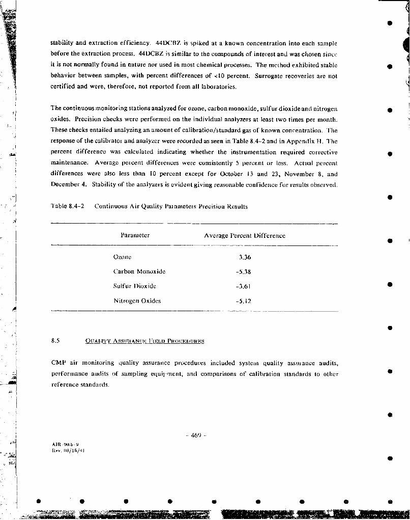
stability and extraction efficiency. 44DCBZ is spiked at a known concentration into each sample

before the extraction process. 44DCBZ is similar to the compounds of interest and was chosen since

it is not normally found in nature nor used in most chemical processes. The method exhibited stable

behavior between samples, with percent differences of <10 percent. Surrogate recoveries are not

certified and were, therefore, not reported from all laboratories.

The continuous monitoring stations analyzed for ozone, carbon monoxide, sulfur dioxide and nitrogen

oxides. Precision checks were performed on the individual analyzers at least two times per month.

These checks entailed analyzing an amount of calibration/standard gas of known concentration. The

response of the calibrator and analyzer were recorded us seen in Table 8.4-2 and in Appendix 11. The

percent difference was calculated indicating whether the instrumentation required corrective,

maintenance. Average percent differences were consistently 5 percent or less. Actual percent

differences were also less than 10 percent except for October 13 and 23, November 8, and

December 4. Stability of the analyzers is evident giving reasonable confidence for results observed.

0

Table 8.4-2 Continuous Air Quality IPaameters Precision Results

Parameter Average Percent Difference

Ozone 3.36

Carbon Monoxide -5,38

Sulfur Dioxide -3.61

Nitrogen Oxides -5.12

8.5 Q- AIIvY ASSURANCE FIELD PI)IO,)IJlRES

CMP air monitoring quality assurance procedures included system quality assurance audits,

performance audits of sampling equilment, and comparisons of calibration standards to otherreference standards.

469 -

AIR -•.A.--

0 • il.081/1 0•Rv 'i

ýIX M

t0

8.5.1 SYSTEM AUDITS

System audits are the external inspection and review of monitoring operation and documentation. 0

"System quality assurance audits of the air 'ampling program for CMP were conducted by the project

quality assurance coordinator. Operations that were audited included sample handling and use of

sample containers or collectors, and documentation. Results were reported to project management

with recommendations for long-term solutions and resolutions to immediate corrective actions. Thes" 0

reports are contained within the project files.

8.5.2 I'"RYORMANCE AUDITS OF F|IELD SAMPLING EqUIlPMENT

Performance audits were performed by personnel independent of the project. The audits consisted

of testing the calibration of samplers with calibration standards other than those used to asse-s daily

operation of the samplelrs.

0

An independent perfoirmance audit was performed quarterly on all field samplers. Detailed results

of the audits can be found in the CMII Quarterly Audit Reports. Summary tables for each audit

report are provided in Appendix II. For each sampler, the operator-determined flow rate was

compared to the auditor flow rate and a percent difference was calculated. The results were 0

compared to EPA guidelines of t7 percent for an acceptable audit result. Field personnel were

informed of any discrepancy and performed the required corrective action for this audit. Corrective

actions were taken immediately and entered in the daily logbook.

0

EPA guidelines were employed to summarize overall accuracy a ag the network of samplers.

Calculation procedures are detailed in the Federal Register, Vol. 51, #53, March 19, 1986. The

procedures call for calculating the average percent difference, standard deviation, and 3:95 percent

confidence limits for all audit points for any p)articular type of sampler in thie moniloring network. 0

Three types of samplers were examined, including TSP samplers, PM-10 samplers, and the

SV()C/OCP samplers. For each type of sampler, the number of audits performed were recorded along

with the iverage percent diffekence and the ±95 percent confidence limits. These were compared to

EPA recommended probability limits of ±20 percent for satisfactory accuracy. Results can be found

in the CMIP Quarterly Audit Reports, with summary tables in Appendix 11.

0

.' .,•! -4'70 -

S" 0 0 S S 0 0 0 0

8.5.3 CALIBRATION AND CERTIFICATION OF STANDARDS

The accuracy of flow calibration equipment was critically important for the type of monitoring

performed in the CMP. Flow rate standards were calibrated against NBS traceable or other

authoritative standards. Appropriate calibration intervals are yearly for the high-volume orifices and

3 to 6 months for the mass flow meter low-volume standards. The high-volume orifices and mass

flow meter standards used in the CMP network were certified and compared to standards contained 0

in the USEPA Region VIII Quality Assurance laboratory.

0

0

-471 -

1(.V. A 8/1 99•. I~Rev, 0(R/Ib/91

-..----...------.- -

S

9.0 CONCLUSIONS

This report focuses on results of the CMP for FY90 and includes analyses and comparisons to data

"for preceding monitoring programs at RMA and for other programs which ran concurrently. The data

were used to characterize the air quality at RMA and also to describe both the impacts of Basin F

remedial activities and the cessation of those activities.

Analyses of these data were used to characterize potential sources for air contaminants which were

observed, including both RMA and metropolitan Denver influences. On-site meteorological data

were also used to describe those conditions associated with the average and the extreme events.

Dispersion modeling was used to evaluate potential sources.

The FY90 program continued the monitoring for similar lompounds which were sampled during the

FY88 and FY89 programs. These include total suspended particulates, PM-10, asbestos, volatile

"o i compounds, semi-volatile organic compounds, organochlorine pesticides, mercury, arsenic,

a 'it ther metals. The following discussion summarizes the results of the analyses for each group of

i ouality parameters.

SI TOTAL SUSPENVFI) I tT

"';iP levels at RMA can be attributed to two principal sources: (i) the influx of particulates from

i;,,politan Denver, and (2) remedial activity sources which help-,d to produce wind-blown dust,

particularly during very dry episodes. Intense remedial activity was initiated during FY88 and

conminued into FY89. These activities were concluded in several steps, including the completion of

intrusive activities (December 12), the completion of the development of the clay caps (February 15),

and the completion of all topsoil remediation activities (May 5). The TSP data clearly reflect the

impact -)f these activities, with dramatic decreases in TSP levels around Basin F and throughout the

Arsenal after the conclusion of remedial activities and in FY90. During the height of the Basin F

activities, the TSP1 levels which could be attributed to remediation activities also decreased

significantly with distance from the basin or activity source. This feature was observed in the FY88

through FY90 data with respect to Basin F activities and other localized remediation work. In •

addition, there were several episodes during which impacts from metropolitan Denver completely

overwhelmed impacts from potential on-site sources. At the eastern and northern boundaries of

RMA, the TSP levels were well below those of metropolitan Denver, and were more representative

of rural conditions. 0

"- 472 -

Alit W.5-9iRev. 8/15/91

' ,2 • •• • •• •6

.1 0............. .... .... 0 .. .. "0... . .. .. . . .. ,0 . . ..... . ...... 6..... .... .

9.2 RESPIRABLE PARTICULATES (PM-- 10)

Respirable particulates are generated by dry windy conditions, but to a much lesser extent than for

TSP. There were no violations of the annual or 24-hour PM-10 standards at RMA during FY90.

There were some increases in PM- 10 levels immediately adjacent to remediation activities; however,

these impacts were highly localized and concentrations decreased significantly at short distances from

the potential source.

9.3 METALS

Ambient concertLnations of metals across RMA were generally proportional to levels of TSP.

Maximum concentrations were sampled on high wind speed days and also when there were high TSP

and PM-10 levels, which in turn were frequently attributed to sources off the Arsenal. During

remediation activities, Basin F appeared to be a source of mercury, chromium, copper and zinc, and

these concentrations decreased rapidly with distance from Basin F. Following remediation of the

basin, the metals levels were reduced to those typical of baseline conditions. During FY89, there were

several instances of high metals concentrations associated with low wind speeds and strong inversion

conditions, with a likely source in the Denver metropolitan area.

9.4 ASBESTOS

Asbestos was not detected at RMA during FY90. There were no detections of asbestos during FY88,

and only 2 days with detections during FY89; results confirm that there is no evident source of

ambient asbestos fibers on RMA.

9.5 VOLATILE ORGANIC COMPOUNDS

During the Basin F remediation, on-site activities appeared to be a source of several volatile organic

compounds, including bicycloheptadiene, dimethyl disulfide, benzene, toluene, and ethylbenzene.

Some of these emissions could have resulted from the emissions from heavy equipment which was

used during remediation. Chloroform was identified near both Basin F and the South Plants. Levels

of VOCs which were attributed to RMA sources during the Basin F remediation period decreased

rapidly with distance from those sources, and levels at RMA boundaries were similar to or less than

those within the urban environment of metropolitan Denver. During FY89 and FY90, many of the

- 473 -AIR-90.6-9Rev. 08/15/91

VOCs attributed to Basin F decreased significantly. During FY90, many of the VOCs measured at

RMA monitoring sites were attributed to close-by off-Arsenal sources, as identified in this renort.

9.6 SEMI-VOLATILE ORGANIC COMPOUNDS

Basin F appeared to be a source of several semi-volatile organic compounds, including aldrin,

dieldrin, and endrin during the Basin F remediation activity period. The highest levels were detected

in the immediate vicinity of Basin F during these remediation efforts. Results from BF2, at the

northeast perimeter of Basin F, showed the highest levels of SVOCs, but at the RMA boundaries,

these levels were reduced to roughly background levels. During the FY89 and FY90 post-remedial

periods, SVOC concentrations were reduced significantly in the vicinity of Basin F and all SVOC

concentrations at other RMA (CMP) monitoring sites were close to background levels.

9.7 ORGANOClLOIlNE PESTICIDES

IO

These compounds were at or near the detection limit at the RMA boundary sites. Highest levels were

sampled during the Basin F remediation effort, and nearest to Basin F itself. Following the

completion of the remp'dial activities, these levels were reduced to near background levels in the

vicinity of Basin F as well.

9.8 CRITERIA POLLUTANTS

* I Ambient concentrations of the criteria pollutants, including sulfur dioxide, nitrogen dioxide, carbonr

* monoxide, and ozone were monitored continuously at RMA dur;ng FY90. Generally, the air quality

at the RMA monitoring location was cleaner than at other sites in the Denver area. The RMA data

showed no violations of any short-term or long-term staddards fcr these pollutants. Episodes with

relatively high concentrations at I'MA Aere related to potential nearby sou.'ces under certain

meteorological conditions. Several of these have been specifically related to typical Denver "brown

cloud" conditions and have bee,. 'eraiified in this report.

9.9 UENERAL INTERPRETATIONS

All data reported in this report must be interpreted, .nd used with full regard to the parameters of the

program. These include sampling frequency, analysi, limitations, and a limited observation period.

The interpretations must also consider any anomalow acleorological (air qitality) conditions as well

j- 74

yN

S!• AIR-9ib-9

, ~Rev,. 08/15i/91

t •

0 00

as possible influences of metropolitan Denver sources on RMA ambient air quality, As more data are

collected under subsequent programs, these conclusions may need to be refined and reinterpreted.

44

7.1•

475 -

Al 11-90 5-9H OR/ 15S S-1

•..

"• ,1flXiEf--

i0

10.0 REFERENCES

American Conference of Governmental Industrial Hygienists (ACGIH). 1986. Threshold LimitValues for Chemical Substances in the Work Environment Adopted by ACGIH. ISBN:0-936712-69-4. Cincinnati, Ohio: American Conference of Governmental IndustrialHygienists.

Citizens Fund. 1990. "Poisons in Our Neighborhoods: Toxic Pollution in Colorado." Washington,D.C.

Code of Federal Regulations, Title 40, Part 50, Appendix G. 1978, 1979. "Reference Method forthe Determination of Lead in Suspended Particulate Matter Collected From Ambient Air."

------ Title 40, Part 50, Appendix B. 1985. "Rý "erence Method for the Determination of SuspendedParticulate Matter in the Atmosphere (Hligh-Volume Method)."

S -------Title 40, Parts 51, 52, 53, and 58. 1987. "Ambient Air Quality Monitoring, Data Reporting,and Surveillance Provisions."

Title 40, Part 50, Appendix J. 1987. Reference Method for the Determination of ParticulateMatter as PM-JO in the Atmosphere.

Colorado Dept. of Health, Air Pollution Control Division. 1983. Ambient Air MonitoringRequirements for the Air Pollution Control Division of the Colorado Department of Health.Denver, Colorado: Colorado Dept. of Health.

"Co1984, 1985, 1986, 1987,. 1988, 1989 and 1990. Colorado Air Quality Data Report. Denver,Colorado: Colorado Dept. of Health.

----- 1987 Emission Permits for Rocky Mountain Arsenal. Denver, Colorado: Colorado Dept. ofHealth.

-- ..... 1990. EISPS Emissions Inventory. Denver, Colorado: Colorado Dept. of Health.

Ebasco Constructors, et al. 1989. "Basin F Interim Action Ciose-Out Safety Report." Final, VolumeI, Contract No. DACA45--87-C-0192. Denver, Colorado: U.S. Army Corps of Engineers.

Edsor., H. 1976. "Candidate Users and the Minimum Credible On-.Site Supplementary ControlSystem." Air Pollution Control Association Conference. Portland, Oregon.

1977. "Real-time, Short-term Air Quality Forecasting." Air Pollution Control As:;ociationConference. Toronto, Canada.

1978. "A Statistical Approach to Real-time, Short-term Air Quality Forecasting." FifthConference on Probability and Statistics in Atmospheric Sciences, American MeteorologySociety. Las Vegas, Nevada.

Environmental Science and Engineering, Inc. (ESE, formerly Environmental Science andEngineering, Inc.). 1987. "Final Technical Plan." Contract Number DAAK- 11-84-D-0016,Task Number 18. Denver, Colorado: U.S. Army Rocky Mountain Arsenal. (RIC"#88203R02)

- 416 -

Revy 08/16•/91

4 0

"6.• O l S • • 0 0 O 0

"_ ,,v ., :-'m• , ' S• • '-•- ••-- ' ''••• ''' ' i " ....... ........ ..... -= .-- -,_ .. .,._ : .• -,:z; •

August 1988. "Air Remedial Investigation, Final Report, Version 3.1." Contract NumberDAAA-I 1-84-D-0016, Task Number 18, .enver, Colorado: U.S. Army Rocky MountainArsenal. (RIC #88263R01)

Federal Register, Volume 51, #53, March 19, 1986.

Hanson, R.L. 1981. "Ambient Air Quality Assessment." No. 43-21-0170-81. Denver, Colorado:U.S. Army Rocky Mountain Arsenal. (RIC #81293R04)

llb,, et al. 1986. "EMAAPCA Symposium on Measurements of Toxic Air Pollutants." Raleigh,North Carolira.

i+0 ional Institute of Occupational Safety and Health (NIOSH). 1984. Manual vf/Analytical Methods,"Method 7300 (Metals)." Washington, D.C.: U.S. Government Printing Office.

1985. NIOSH Pocket Guide to Chemical Hazards. Washington, D.C.: U.S. GovernmentPrinting Office.

1987. Manual of Analytical Meth (is. "Method 7400, Revision No. 2 (Asbestos)." Washington,D.C.: U.S. Government Printing Office.

.d Space Technology Laboratories. 1980. "Rocky Mountain Arsenal Contamination SourceControl Study Team at Computer Sciences Corporation." NSTL Station, Mississippi.Engineering Laboratory, Conference Report. (RIC #85213R03)

il, E., Dernian, B., and Krost, K. 1984. Sampling of Organic Compounds in the Presence ofReactive Inorganic Gases with Tenax0 GC. Analytical Chemistry, 56(4), 793-798.

"I'MkMA Certified Analytical Methods." April, 1990.

I'IPIA. "Chemical Qwudity Assurance Plan." Version 1.0, July, 1989. (RIC #89244R01)

la 1 .j(t and Marcero. 1976. "Improved 1 lopcalite Procedure for the Determination of Mercury Vaporin Air by Flamelvss Atomic Absorption." AIHA Journal.

Stollar & Associates, Inc. (Stollar). 1990. "Final Technical Plan for Air Quality." Contiact No.DAAAI5-87--0095. Denver, Colorado: U.S. Army Rocky Mountain Arsenal. (RIC#901 90R02)

'', ;tollar & Associates, Inc. (Stollar). 1988. "Station Operating and Quality Assurance Procedures

for the Continuous Air Quality/Meteorological Parameters Monitoring Station for RockyMountain Arsenal." February 1988.

"988. "Field Procedures Manual for the Comprehensive Monitoring Program." Denver,Colorado: U.S. Army Rocky Mountain Arscnal.

- 1988. "Draft Final Technical Piau for Air Quality." Contract No. DAAA 15-87-0095. Denver,Colorado: U.S. Army Rocky Mountain Arsenal.

R. L. Stollar & Associates, Inc. (Stollar). 1990. "Air Quality Data Assessment Report for theComprehensive Monitoring Program." Contract No. DAAA15-87-0095. Denver, Colorado:U.S. Army Rocky Mountain Arsenal. (RIC #90190R01)

-477 -AIR 90.6-9Rev' EMJ/if/fl

0' 0

S....... ..

I R.L. Stollar & Associates, Inc. (Stollar). 1990. "A'- Quality Data Assessment Report for theComprehensive Monitoring Program." Contrac, No. DAAA15-87-0095. Denver, Colorado.U.S. Army Rocky Mountain Arsenal. (RIC #90230R01)

0"U.S. Army Corps of Engineers, Waterways Experiment Station. 1982. "Basin F Overburden and Soil

Sampling Analysis Study." Commerce City, Colorado: U.S. Army Rocky Mountain Arsenal.(RIC #82350R01)

U.S. Army Environmental Hygiene Agency. 1969. "Air Pollution Engineering AtmosphericBackground Study." No.21-005-70. Commerce City, Colo ido: U.S. Army Rocky MountainArsenal. (RIG #85184R02)

------. 1982. "Evaluation of Organic Vapor Emissions, Basin F, Rocky Mountain Arsenal," Parts Iand 2. USAEItA Project No. 43-21-0230-83. Commerce City, Colorado: U.S. Army RockyMountain Arsenal. (RIG #82347R02 and #83192R02)

U.S. Dept. of Commerce. 1988. "National Air Toxics Information Clearinghouse (NATICHI) Database

Report on State, Local, and EPA Air Toxics Activities." PB89-106983. Austin, Texas:Radian Corporation.

U.S. Environmental Protection Agency (U.S. EPA). 1976. Quality Assurance Handbook for AirPollution Measurement Systems, Vol. 1, "Principles." EPA-600/9-76-005. Research TrianglePark, North Carolina: U.S. EPA Office of Research and Development.

- ----- 1983. "Methods for Chemical Analysis of Water and Wastes (Method 206.2)." EPA-600/4-79-020. Research Triangle Park, North Carolina: U.S. EPA Office of Research andDevelopment. (RIG #87181R01)

- ----- 1983. Test Method, Section 2.2, Reference Method for the Determination of SuspendedParticulates in the Atmosphere (High Volume Method). EPA-600/4.-77-027a. ResearchTriangle Park, North Carolina: U.S. EPA Office of Research and Development.

"Meteorological Instruments." EPA-600/4-82-060. Research Triangle Park, North Carolina:

U.S. EPA Office of Research and Development.

- ----- 1984. Compendium of Methods for the Determination of Toxic Organic Compounds in AmbientAir (Method TO-f, Method TO-4, Method 608). EPA-600/4-84-041. Research TrianglePark, North Carolina: U.S. EPA Office of Research and Development.

*1985. Quality Assurance Handbook for Air Pollution Measurement Systems, Vol. I1, "AmbientAir Specific Methods." EPA-600/4-77/027a. Research Triangle Park, North Carolina: U.S.EPA Office of Research and Development.

- 1986. Industrial Source Complex (ISC) Dispersion Model User's Guide, Vol. L., 2nd. Ed. EastHartford, Connecticut: TRC Environmental Consultants. 0

---- 1986. 1NPUFF2 Dispersion Model User's Guide. EPA-600/8-86-024.

1986. Superfund Public Health Evaluation Manual. EPA-540/I-86.-060. Washington, D.C.:Office of Emergency and Remedial Response, Office of Solid Waste and EmergencyResponse. (RIC #91018R01) 0

- 478 -

Rev. 08/15/91

0 w 0 p 49 0

A --- -•1

----- 1987. "Ambient Monitoring Guidelines for Prevention of Significant Deterioration (PSD)."EPA-450/4-87-007. Research Triangle Park, North Carolina: U.S. EPA Office of Air andWaste Management, Office of Air Quality Planning and Standards.

- ----- 1988. 1987 Nonmethane Organic Compound and Air Toxics Monitoring Program, FinalReport, Vol. II, "Toxic Species". EPA-450/4-88-012. Research Triangle Park, NorthCarolina: U.S. EPA Office of Research and Development.

------ 1989. Report on the Air Toxics Monitoring Program for the Denver Metropolitan Area.Integrated Environmental Management Pro, Report One, Data Summary. Region VIII,

,7• Denver, Colorado.

Walling, J.F., et al. 1986. "Apparent Reaction Products Desorbed from Tenaxo Used to SampleAmbient AiL." Atmospheric Environment, 20(1), 51-57.

Weatherbank, Inc. 1990. Denver (Stapleton Airport) meteorological data for September, 14, 1990."Salt Lake City, UT.

Witt, M.E. 1978. Memorandum for Record, Basin A Dust Sample. Commerce City, Colorado: U.S.Army Rocky Mountain Arsenal.

0

i0

I

'1

479 -A1lt-90.5-9

Rlev. 08/15/91

- 0JfC

UN SFIED4

UNCLASSIFIAED

Or... .....

re' ad-a286 896 page form approvedno. · 4.7.4 summary of results and assessment of svo(...

Documents