RE-CONCEPTUALIZING JOINT ATTENTION AS SOCIAL

SKILLS: A MICROGENETIC ANALYSIS OF THE DEVELOPMENT OF EARLY INFANT COMMUNICATION

by

Maximilian B. Bibok B.A. Honours, University of Victoria, 2005

M.A., Simon Fraser University, 2007

DISSERTATION SUBMITTED IN PARTIAL FULFILLMENT OF THE REQUIREMENTS FOR THE DEGREE OF

DOCTOR OF PHILOSOPHY

In the Department of Psychology

© Maximilian B. Bibok 2011

SIMON FRASER UNIVERSITY

Spring 2011

All rights reserved. However, in accordance with the Copyright Act of Canada, this work may be reproduced, without authorization, under the conditions for Fair Dealing. Therefore, limited reproduction of this work for the purposes of private study, research, criticism, review and news reporting is likely to be in

accordance with the law, particularly if cited appropriately.

ii

APPROVAL

Name: Maximilian B. Bibok

Degree: Doctor of Philosophy

Title of Thesis: Re-Conceptualizing Joint Attention As Social Skills: A Microgenetic Analysis Of The Development Of Early Infant Communication

Examining Committee:

Chair: Dr. Grace Iarocci Associate Professor

______________________________________

Dr. Jeremy I. M. Carpendale Senior Supervisor Professor

______________________________________

Dr. Timothy Racine Supervisor Assistant Professor

______________________________________

Dr. Kathleen Slaney Supervisor Assistant Professor

______________________________________

Dr. Jeff Sugarman Internal External Examiner Professor

______________________________________

Dr. Vasudevi Reddy External Examiner Professor University or Portsmouth

Date Defended/Approved: April 7, 2011

Last revision: Spring 09

Declaration of Partial Copyright Licence The author, whose copyright is declared on the title page of this work, has granted to Simon Fraser University the right to lend this thesis, project or extended essay to users of the Simon Fraser University Library, and to make partial or single copies only for such users or in response to a request from the library of any other university, or other educational institution, on its own behalf or for one of its users.

The author has further granted permission to Simon Fraser University to keep or make a digital copy for use in its circulating collection (currently available to the public at the “Institutional Repository” link of the SFU Library website <www.lib.sfu.ca> at: <http://ir.lib.sfu.ca/handle/1892/112>) and, without changing the content, to translate the thesis/project or extended essays, if technically possible, to any medium or format for the purpose of preservation of the digital work.

The author has further agreed that permission for multiple copying of this work for scholarly purposes may be granted by either the author or the Dean of Graduate Studies.

It is understood that copying or publication of this work for financial gain shall not be allowed without the author’s written permission.

Permission for public performance, or limited permission for private scholarly use, of any multimedia materials forming part of this work, may have been granted by the author. This information may be found on the separately catalogued multimedia material and in the signed Partial Copyright Licence.

While licensing SFU to permit the above uses, the author retains copyright in the thesis, project or extended essays, including the right to change the work for subsequent purposes, including editing and publishing the work in whole or in part, and licensing other parties, as the author may desire.

The original Partial Copyright Licence attesting to these terms, and signed by this author, may be found in the original bound copy of this work, retained in the Simon Fraser University Archive.

Simon Fraser University Library Burnaby, BC, Canada

STATEMENT OF ETHICS APPROVAL

The author, whose name appears on the title page of this work, has obtained, for the research described in this work, either:

(a) Human research ethics approval from the Simon Fraser University Office of Research Ethics,

or

(b) Advance approval of the animal care protocol from the University Animal Care Committee of Simon Fraser University;

or has conducted the research

(c) as a co-investigator, collaborator or research assistant in a research project approved in advance,

or

(d) as a member of a course approved in advance for minimal risk human research, by the Office of Research Ethics.

A copy of the approval letter has been filed at the Theses Office of the University Library at the time of submission of this thesis or project.

The original application for approval and letter of approval are filed with the relevant offices. Inquiries may be directed to those authorities.

Simon Fraser University Library

Simon Fraser University Burnaby, BC, Canada

Last update: Spring 2010

iii

ABSTRACT

The present longitudinal study examined how 28 infants’ joint attention behaviours undergo developmental change across the 9 to 12 month age range. Two competing theoretical views of the development of infants’ joint attention are the cognitivist and skill-based conceptualizations of social cognition. The present study reviews and discusses the conceptual differences between these two approaches in detail. Starting from the operational definition of joint attention the differences between these two conceptualizations of infants’ social cognition are explicated. It will be shown that each framework operates from a different set of assumptions regarding the development of joint attention behaviours. In turn, it will be argued that these assumptions naturally lend themselves to different metrics of behavioural measurement and programmes of research. The central tenets of the skill-based conceptualization of social cognition are presented and contrasted with those of the cognitivist framework. Empirical research situated within the cognitivist framework is examined and discussed in light of the differences between these two conceptualizations of joint attention. Following from this review, the rationale and purpose for the present study is described, and the study presented.

Prior research has established that beginning around 9 months of age infants’ joint attentional behaviours increase in frequency. Less research, however, has been conducted to investigate how the temporal characteristics of infants’ joint attention behaviours change with development. Infants’ joint attentional abilities were assessed using the Early Social Communication Scale (ESCS). Contingency scores produced by T-pattern analysis, wherein infants’ joint attention behaviours contingently followed object specific events (e.g., an active toy object), were found to undergo changes in frequency, timing, and probability of occurrence across the months of assessment. Implications of these results for a skill-based conceptualization of joint attention are discussed.

Keywords: Joint attention; skill theory; infant development; sequential analysis

iv

ACKNOWLEDGEMENTS

First and foremost, I wish to thank my senior supervisor, Dr. Jeremy Carpendale, for his support and guidance throughout this project. His personal dedication and commitment to grappling with foundational issues central to developmental psychology, and which other academics would rather simply avoid, has afforded me numerous hours of productive and stimulating conversation over the course of my studies. It is against this backdrop of intellectual exchange that this project was completed. I also wish to thank my other committee supervisors, Dr. Timothy Racine and Dr. Kathleen Slaney, for their many constructive and thoughtful comments throughout this project. I am thankful to Dr. Raymond Koopman for the many hours of assistance and advice he provided me on the statistical component of this project. Finally, I wish to thank Ruby Grewal for her conscientiousness and diligence in helping me establish inter-rater reliability.

v

TABLE OF CONTENTS

Approval ............................................................................................................................ ii Abstract ............................................................................................................................ iii Acknowledgements .......................................................................................................... iv Table of Contents .............................................................................................................. v List of Figures.................................................................................................................. vii List of Tables ...................................................................................................................viii

Introduction....................................... ...............................................................................1 Definition of Joint Attention................................................................................................2 Joint Attention and the Need for “Checking”......................................................................3 Rich Interpretation .............................................................................................................5

Ontogenetic Ritualization ..........................................................................................6 Lean Interpretation ............................................................................................................7 Motivational Issues............................................................................................................8 Joint Attention and Re-Description....................................................................................8 Communicative Intent........................................................................................................9 Communicative Signal Conceptualization of Behaviour ..................................................11 Events are Atemporal ......................................................................................................13 Consequences of a Cognitivist Conceptualization of Joint Attention –

Present/Absent Dichotomy......................................................................................14 “Understanding” versus “Understand” .............................................................................15 Depth or Breadth of Understanding.................................................................................16 Studies Utilizing Frequency Scores of Joint Attention .....................................................18

Parlade et al., 2009; Venezia et al., 2004 ...............................................................18 Mundy et al., 2007...................................................................................................19 Bakeman & Adamson, 1984 ...................................................................................20

Joint Attention and Frequency Counts ............................................................................20 Researching Joint Attention – Individual Differences in the Development of Joint

Attention ..................................................................................................................24 Sensorimotor Conceptualization of Behaviour ................................................................25 Skill-Based Approach to the Study of Joint Attention ......................................................27

Skills Permit Continuous Metrics.............................................................................30 Skills Involve Practice .............................................................................................30 Skills Focus on Practical Activities ..........................................................................30 Skills are Intrinsically Temporal...............................................................................31 Skills Metrics ...........................................................................................................32

Summary .........................................................................................................................33 Purpose of the Current Study..........................................................................................34

Method............................................. ...............................................................................37 Participants......................................................................................................................37 Materials ..........................................................................................................................37

vi

Early Social Communication Scale (ESCS) ....................................................................38 Procedure........................................................................................................................39 Video Coding...................................................................................................................39 Behavioural Codes ..........................................................................................................40 Inter-rater Reliability ........................................................................................................40 Data Reduction of Behavioural Codes ............................................................................41 Parameter Issues Involved in Data Reduction Procedure...............................................43 Exclusion of Multiple Hypotheses – Analyzing all Pair-wise Combinations.....................44 Descriptive Measures Resulting from Data Reduction Procedure ..................................45 Data Mining Procedure....................................................................................................46 Non-Parametric Tests and Power Analysis .....................................................................52 Generalizability of Exploratory Research ........................................................................53

Results and Discussion............................. ...................................................................55 Data Mining Procedure and Type I Error Control ............................................................55 Data Analytic Strategy and Result Discussion ................................................................55 Descriptive Statistics .......................................................................................................58 Zero-Order Correlations ..................................................................................................58 Initiating Joint Attention ...................................................................................................59

Primary Analysis – Initiating Joint Attention ............................................................59 Secondary Analysis – Initiating Joint Attention........................................................66 Discussion – Initiating Joint Attention......................................................................71

Initiating Behavioural Response......................................................................................74 Primary Analysis – Initiating Behavioural Response...............................................74 Secondary Analysis – Initiating Behavioural Response ..........................................83 Discussion – Initiating Behavioural Response ........................................................88

Responding to Behavioural Response ............................................................................91 Primary Analysis – Responding to Behavioural Response .....................................91 Secondary Analysis – Responding to Behavioural Response ................................94

General Discussion................................. ......................................................................95

Reference List..................................... .........................................................................102

Appendices ......................................... .........................................................................110 Appendix A: Behavioural Codes...................................................................................111 Appendix B: Description of Monte Carlo Procedure .....................................................125 Appendix C: Descriptive Statistics................................................................................134

vii

LIST OF FIGURES

Figure 1. Audio waveform of an active mechanical toy (vertical bars denote onset and offset) ...........................................................................................111

Figure 2. Audio waveform of experimenter talking (“Wanna see it”) (vertical bars denote onset and offset) ...............................................................................113

Figure 3. Audio waveform of verbal command (“Can I have it?”) (vertical bars denote onset and offset) ...............................................................................115

Figure 4. Example of fast intervals (topmost connectors) and free intervals (bottommost connectors) between two codes on a discrete interval time-line (Magnusson, 2000, p. 97) ..............................................................129

viii

LIST OF TABLES

Table 1 Mean Kappas for Infant Behavioural Codes for Two Random Participants Across 9, 10, 11, and 12 Months ....................................................................42

Table 2 Correlations Within Standard ESCS Composite Score ......................................60

Table 3 Correlations Across Standard ESCS Composite Scores ...................................61

Table 4 Correlations Within Individual Standard ESCS Behavioural Codes ...................62

Table 5 Correlations Between IJA Eye Contact and IJA Show Standard ESCS Behavioural Codes..........................................................................................65

Table 6 Correlations Across Descriptor Classes of Infant Gaze Behavioural Contingencies Contextualized to Active Object Spectacle Extended .............67

Table 7 Correlations Across Descriptor Classes of Infant Gaze Behavioural Contingencies Contextualized to Infant Toy Touch ........................................69

Table 8 Correlations Across Descriptor Classes of Infant Gaze Behavioural Contingencies Contextualized to Active Object Spectacle Extended and Infant Toy Touch ......................................................................................70

Table 9 Mean Difference Tests of IBR Lower, Higher, and Total Composite Standard ESCS Behavioural Frequency Scores ............................................75

Table 10 Mean Difference Tests of IBR Give With Gaze, IBR Give Without Gaze, and IBR Appeal Standard ESCS Behavioural Frequency Scores ..................77

Table 11 Correlations Between IBR Give With Gaze and IBR Give Without Gaze Standard ESCS Behavioural Codes ...............................................................78

Table 12 Mean Difference Tests of IBR Give Without Gaze ESCS Behavioural Sequential Contingencies ...............................................................................79

Table 13 Correlations Across Descriptor Classes of IBR Give With Gaze and IBR Give Without Gaze ESCS Behavioural Sequential Contingencies .................80

Table 14 Mean Difference Test of IBR Give With Gaze and IJA Alternate Standard ESCS Behavioural Frequency Scores ............................................82

Table 15 Mean Difference Tests of Frequency of Infant Reach Base Behaviour Contextualized to Active Object Spectacle Extended .....................................84

Table 16 Correlations Across Descriptor Classes of Infant Gaze and Infant Reach Behavioural Contingencies Contextualized to Active Object Spectacle Extended ........................................................................................86

Table 17 Mean Difference Tests of Frequency of Infant Reach and Infant Gaze Base Behaviour Contextualized to Inactive Object Spectacle ........................87

ix

Table 18 Mean Difference Tests of Infant Give Base Behaviour Contextualized to Infant Toy Touch .............................................................................................89

Table 19 Mean Difference Tests of RBR Total Fail and RBR Total Pass Standard ESCS Behavioural Frequency Scores ............................................................92

Table 20 Mean Difference Tests of RBR Pass With Gesture and RBR Pass Without Gesture Standard ESCS Behavioural Frequency Scores .................93

Table C1 Descriptive Statistics of Standard ESCS Behavioural Frequency Scores .....134

Table C2 Descriptive Statistics for ESCS Behavioural Contingencies ..........................138

1

INTRODUCTION

Considerable research has been conducted on the development of infants’ joint attentional abilities (e.g., Adamson & Bakeman, 1984; Bakeman & Adamson, 1984; Carpenter, Nagell, & Tomasello, 1998; Corkum & Moore, 1995; Leung & Rheingold, 1981; Liszkowski, Carpenter, Henning, Striano, & Tomasello, 2004; Liszkowski, Carpenter, & Tomasello, 2007; Moore & Corkum, 1994; Morales, Mundy, Crowson, Neal, & Delgado, 2005; Morales, Mundy, Delgado, Yale, Messinger, Neal, & Schwartz, 2000; Mundy, Block, Vaughan Van Hecke, Delgado, Venezia Parlade, & Pomares, 2007; Mundy & Gomes, 1998; Parise, Cleveland, Costabile, & Striano, 2007; Parlade, Messinger, Delgado, Kaiser, Van Hecke, & Mundy, 2009; Striano & Rochat, 1999; Van Hecke et al., 2007; Venezia, Messinger, Thorp, & Mundy, 2004). Typically, joint attention is conceptualized within a cognitivist framework, according to which the development of joint attention is a consequence of infants’ understanding of others as intentional agents (Tomasello, 1995; Tomasello, Carpenter, Call, Behne, & Moll, 2005; Tomasello, Carpenter, & Liszkowski, 2007). However, it has been argued that joint attention may be alternately conceptualized as an interactive social skill (Mundy & Gomes, 1997; Mundy & Sigman, 2006; Van Hecke & Mundy, 2007). Under this view infants’ joint attentional abilities arise out of the social practices that they participate in during the first two years of development (Bibok, Carpendale, & Lewis, 2008; Carpendale & Lewis, 2004, 2006; Racine & Carpendale, 2007).

The present study builds upon this work by investigating how across the 9 to 12 month age range specific forms of infants’ joint attention behaviour undergo microgenetic developmental change: the analysis of individual developmental transitions in abilities over short time spans within a specific developmental domain (Flynn, Pine, & Lewis, 2007). Prior research (Carpenter et al., 1998; Mundy et al., 2007) has established that beginning around 9 months of age infants’ joint attentional behaviours increase in frequency. Less research, however, has been conducted to investigate how infants’ real-time execution of joint attention behaviours undergoes development changes. According to the skill-based conceptualization of joint attention, the development of joint attentional abilities may be indexed by changes in the speed and efficiency of behavioural production, as well as changes in base frequency (Mundy, Sullivan, & Mastergeorge, 2009). Under the cognitivist conceptualization of joint attention,

2

however, such changes in the production of behaviour are considered irrelevant to understanding the development of infant’s social cognition. Such microgenetic changes are likely to be interpreted as representing extraneous performance factors rather than the core social cognitive competency under investigation.

There exists, therefore, a deep theoretical division between the cognitivist and the skill-based conceptualizations of social cognition. In order to theoretically situate the present study it is necessary to review and discuss this division in some detail. Starting from the operational definition of joint attention the following review will explicate the differences between these two conceptualizations of infants’ social cognition. It will be shown that each framework operates from a different set of assumptions regarding the development of joint attention behaviours. In turn, it will be shown that these assumptions naturally lend themselves to different metrics of behavioural measurement and programmes of research. Within the context of this discussion, the central tenets of the skill-based conceptualization of social cognition will be presented and contrasted with those of the cognitivist framework. Empirical research situated within the cognitivist framework will be examined and discussed in light of the differences between these two conceptualizations of joint attention. Finally, from this discussion, the rationale and purpose for the present study will be described, and the study presented.

Definition of Joint Attention

Behaviourally defined, episodes of joint attention, or "joint visual attention" (Moore & Corkum, 1994, p. 350), consist of those instances in which two actors each sensorially orient toward the same aspect of the environment (typically an object). Operationally this means, “looking where someone else is looking” (Butterworth, 1995, p. 29). Nevertheless, this minimalist definition (Racine & Carpendale, 2007) does not capture the cognitive aspects of the concept in which most researchers are interested. Many researchers (Tomasello et al., 2007) take the position that joint attention is psychologically defined by two persons both attending toward the same aspect of the environment, with each knowing that the other is attending as well. That is, two persons are “jointly” (i.e., together) attending psychologically toward the same aspect of the environment.

Starting between 6 and 8 months of age children develop nonverbal communications skills that are functionally distinct (Mundy & Gomes, 1997). At around 9 months of age joint attention first appears during infant development. However, it is not until 12 months of age and older that it becomes a regular feature of infants’ social communicative repertoire (Carpenter et al., 1998). Of the various forms of joint attention behaviours that infants engage in during this

3

time period (e.g., social referencing, following pointing gestures), two functionally distinct behavioural forms of joint attention that have received considerable research interest are (a) imperative and (b) declarative joint attention behaviours. Imperative forms of joint attention designate those socially interactive behaviours in which infants make requesting and/or commanding gestures (e.g., reaching, whining, pointing) so as to elicit the help of a partner in obtaining an object. The defining feature of imperative joint attention behaviours is that they signify to the partner that the infant wants him or her to “do” something (Carpenter et al., 1998, p. 3). Imperative forms of joint attention have also been referred to as “initiating behavioural requests” (IBR: Seibert, Hogan, & Mundy, 1982, 1987). Declarative joint attention behaviours designate those actions in which infants direct the attention of a social partner in order to demonstrate or point out some aspect of the environment or situation for the purpose of sharing attention with the social partner. In contrast to imperative joint attention behaviours, declarative behaviours are about changing the focus of the social partner’s attention and not his or her behaviour (Carpenter et al., 1998). Declarative forms of joint attention have also been referred to as “initiating joint attention” (IJA: Seibert et al., 1982, 1987).

Within the constellation of declarative behaviours, Tomasello and colleagues (2007) have recently drawn a distinction between expressive and informative declarative behaviours. Expressive declarative joint attention behaviours are aimed at getting the social partner to “feel” something (p. 714). A frequent example of infants’ expressive declarative behaviour is the holding up of a toy at eye level and shaking it so as to draw the attention of the social partner toward the toy. Typical of joint attention behaviours, this toy shaking behaviour appears in development around 9 month of age, and increases substantially in frequency around 10 to 13 months of age (Carpenter et al., 1998; Mundy, Delgado, Block, Venezia, Hogan, & Seibert, 2003). Informative declarative joint attention behaviours are aimed at helping social partners complete some action by informing them about objects or aspects of the environment. An example would be pointing toward an object that someone is actively trying to locate.

Joint Attention and the Need for “Checking”

As previously stated, on the level of observable behaviour, joint attention takes the form of two individuals sensorially orienting (e.g., looking) toward the same object. However, many researchers view this behavioural definition as insufficient. On it own, this definition is viewed as incapable of shedding light on what infants understand of the social world. That is, alternate, non-cognitive explanations of joint attention behaviour (i.e., “behaviourist” explanations) cannot

4

be ruled out prima facie. For instance, infants’ gaze toward a social partner may be elicited by the partner’s movement; hence, infants are responding behaviourally, and not psychologically, toward the partner. It is difficult, therefore, under the minimalist definition to interpret from infants’ joint attention behaviours what they understand about their social partners. Consequently, some researchers have added a further definitional stipulation that each actor must not only orient toward the same object, but also check that the other is also attending to the same object or event (Carpenter et al., 1998; Mundy et al., 2003). Specifically, the act of checking on the part of infants allows researchers a degree of confidence that the gaze toward a social partner did not occur by chance, accident, or distraction, but represents self-generated behaviour (Carpenter et al., 1998). This distinction between environmentally driven and self-generated joint attention behaviour has been referred to as the difference between an “alternation of attention” and a “coordination of attention,” respectively (Carpenter et al., 1998, p. 6).

This extra definitional caveat of “checking,” as it has been called (Moore & Corkum, 1994, p. 352), constitutes one of the greatest sources of friction in theoretical discussions regarding joint attention (Moore, 1998; Moore & Corkum, 1994; Tomasello, 1995; Tomasello et al., 2007). Specifically, checking has been construed as a way of observationally assessing whether infants have an understanding of others as intentional agents: i.e., agents who have a psychological orientation toward the world, and thus whose attention can be directed (Carpenter et al., 1998; Tomasello et al., 2005; Tomasello et al., 2007). In contrast, checking has also been interpreted as merely fulfilling a behavioural role in a coordinated chain of socially interactive behaviours that collectively constitute joint attention (Moore & Corkum, 1994). In such instances, checking demonstrates that infants recognize that social partners do not behave (perform) as expected if their eyes are not oriented toward the object involved in the interaction. Specifically, infants recognize a behavioural association between the gaze direction of others and their actions. This behavioural association, however, is said to be not understood by infants as stemming from a relation between the actions of others and their intentions (Gomez, Sarria, & Tamarit, 1993, as cited in Carpenter, 1998, p. 18). Aside from this stipulation, there is general consensus amongst researchers that two individuals orienting toward the same event is a necessary, though potentially insufficient, condition for the ascription of joint attentional abilities.

The issue of checking, therefore, alludes to the central theoretical debate in the literature on joint attention: how best to theoretically interpret the fact that two individuals are capable of behaviourally/sensorially orienting toward the same event (object). Two overarching points of view have arisen to date: rich

5

and lean interpretations of joint attention. In the context of this debate, the adjectives “rich” and “lean” refer to the degree to which infants have an “adult-like” (Tomasello et al., 2005) understanding of others as intentional agents.

Rich Interpretation

Advocating a rich interpretation of joint attention behaviours, Tomasello and colleagues assume that infants’ ability to engage in joint attention behaviours rests upon their understanding of others as intentional (purposeful and goal directed) agents (Carpenter et al., 1998; Tomasello, 1995; Tomasello et al., 2005; Tomasello et al., 2007). It is this understanding of others’ intentionality that allows infants to coordinate their behaviours with those of others. That is, the reason infants behave as to direct the attention of others is that they understand others as having a psychological (intentional) relation to the world that can be directed/influenced. To quote Tomasello and colleagues (2007, p. 716) at length (the logical circularity of this account will be addressed later):

So why do infants not learn to use the extended index finger for these social functions at 3-6 months of age, but only at 12 months of age? Our basic answer is that 3- to 6-month-old infants do not point for others communicatively because communicative pointing requires at least some implicit understanding of the formula she intends that I attend to X (and wants us to know this together) for some reason relevant to our common ground. Infants do not yet have the requisite understanding of intentions, attention, and shared attention and knowledge – nor the requisite motivations for cooperation and helping. As soon as they acquire these competencies and motivations infants begin pointing for others communicatively, suggesting some connection.

From this selection, it can be seen that the understanding of others as intentional agents serves a causal role in the production of infants’ joint attention behaviours. This purported understanding is considered to be “the most important feature [of joint attention] from a social-cognitive point of view” (Carpenter et al., 1998, p. 5). Moreover, under this model all the different forms/manifestations of joint attention (e.g., directives, imperatives, informative, etc.) result from this understanding (Carpenter et al., 1998; Tomasello et al., 2007). That is, the various forms of joint attention exhibited by infants are seen as symptomatic of their understanding others as intentional agents: “our main concern here is to identify the age at which infants seem to engage in these behaviors in a way that indicates [italics added] some understanding of the

6

adult's psychological relation or attention to the outside world” (Carpenter et al., 1998, p. 8). Consequently, this model assumes developmental synchronies in the various forms of joint attention behaviour; i.e., they should all appear at approximately the same time in ontogenetic development, somewhere between 9 and 15 months of age (Carpenter et al., 1998). It follows from this view that there should exist theoretically a strong divide between behaviour and understanding: Understanding, according to this view, is manifested through behaviour, but is not intrinsic to behaviour.

Ontogenetic Ritualization

A further facet of Tomasello and colleagues’ rich interpretation of joint attention that reflects a strong conceptual division between behaviour and understanding is the notion of “ontogenetic ritualization” (Carpenter et al., 1998). Ontogenetic ritualization refers to infants’ capacity to learn certain idiosyncratic gestures through their consistent, frequent, and replicable usage in social interactive contexts. Essentially, the term refers to instrumental/operant learning. A frequently employed illustration is infants who hold their hands above their heads to gesture to be picked up by their caregiver (Carpenter et al., 1998). Ontogenetic ritualization, therefore, demarcates those socially interactive behaviours that infants learn to perform, and which do not require them to understand others as intentional agents. It follows from Tomasello and colleagues’ position that infant joint attention behaviour is defined solely in terms of infants’ purported psychological understanding of others’ intentionality. Joint attention behaviour is not defined functionally, physically, or morphologically, but instead psychologically – i.e., some unobservable, indefinable, ineffable, unquantifiable quality. The phenomenon being investigated, under Tomasello and colleagues’ account, therefore, is not joint attention behaviour, per se, but infants’ psychological understanding of others (Tomasello, 1995).

The notion of “ontogenetic ritualization” seems to constitue a contradictory element in Tomasello and colleagues’ account of joint attention behaviours. Supposedly, any gesture acquired through ontogenetic ritualization (instrumental learning), although communicative, does not count as a full fledged instance of joint attention. The reason for this is that any instance of joint attention must behaviourally display some property that permits the inference that the infant understands something about the intentional state of the social partner. However, an infant gesture, such as the “arms up” gesture, is just as socially efficacious as one purported to require understanding the intentionality of others. In terms of explanatory potential, what is gained by appeals to an understanding of intentionality in explaining infants’ joint attention behaviour? Put differently,

7

from the point of the view of the infant, there is no material (physical) difference between psychologically driven joint attention behaviours and behaviours resulting from ontogenetic ritualization. Thus, to maintain the distinction between these two forms of socially interactive behaviours, it would be necessary to establish that psychologically based joint attention behaviours could not occur in the absence of a purported psychological understanding.

Lean Interpretation

In contrast to the rich interpretation or “commonsense view” of infants’ joint attention abilities proposed by Tomasello and colleagues, Moore and Corkum (1994, p. 350) advocate a lean interpretation of such behaviours. They argue that such behaviours can arise from “instrumental conditioning” (Moore & Corkum, 1994, p. 353) and other forms of behavioural regulation, such as attentional cueing (Moore, 2007). That is, infants’ joint attention behaviours, although socially coordinated with others, do not necessarily suggest that infants have an understanding of others as intentional agents. Rather, infants understand others as causal agents. For instance, Moore and Corkum (1994, p. 358) suggest that declarative joint attention behaviours, rather than directing the attention of others, have the aim of drawing attention to the self. Similarly, Moore and D’Entremont (2001) have suggested that infants use joint attention behaviours to enrich their interactive experience with their social partners, rather than to influence their partners’ attentional states. Only later on in development do infants construct knowledge of others as intentional agents, based upon their earlier social interactions (Moore & Corkum, 1994). One suggestion as to how this occurs may be that infants use the correlations and latencies (contingencies) between social interactive events to build this understanding (Moore & Corkum, 1994). These contingencies are used by infants to coordinate their private first-person information with the third-person information they observe about others (Barresi & Moore, 1996; Moore, 1996). From this matching relation between first and third-person perspectives, infants are then able to imagine the first-person perspective of others, thereby coming to understand them as intentional agents.

Moore and colleagues (Moore & Corkum, 1994; Moore & D’Entremont, 2001) argue that given the nature of observational data, the potential to interpret an infant behaviour either richly or leanly always remains an open possibility. This fact is also acknowledged by Tomasello (1995). Moore and colleagues argue that prima facie there is no inherent reason why theoretical consideration should be given preferentially to rich interpretations of joint attention that posit “adult-like” psychological states on the part of infants. Furthermore, they point to the fact that numerous rich interpretations of joint attention assume that infants’

8

purported ability to understand others as intentional agents is innate (Moore & Corkum, 1994). Due to the unconstrained nature of observational data (i.e., scientific underdetermination), Moore and Corkum call for the need for more experimental research or a “critical hypothesis-testing approach” toward joint attention (Moore 1998; Moore & Corkum, 1994).

Motivational Issues

In both Tomasello’s and Moore’s accounts, it is apparent that central to each account is the assumption that behaviour is simply a syndrome or manifestation of an underlying mental state. What each approach debates is the nature of the purported mental phenomenon lying behind, and giving rise to, the behavioural phenomenon. Considered in a different sense, what each approach disputes is the nature of infants’ motivation to engage in joint attention behaviours (cf. Tomasello et al., 2007; Rakoczy, 2007). That is, each approach attempts to address the question, “Why do infants share attention and experiences with others?” as opposed to the question of “How are infants able to share attention and experience with others?” (Mundy & Sigman, 2006, p. 313). Do infants perform joint attention behaviours because they (a) understand others as causal agents – Moore and colleagues’ interpretation; or (b) understand others as intentional agents – Tomasello and colleagues’ interpretation? The idea at work here is that as infants only engage in these behaviours in the presence of social partners (Butterworth, 1998), what psychological orientation do infants take toward their interactive partners? What these two theoretical approaches to joint attention focus upon are the possible interpretations of infants’ epistemic knowledge of social partners, given infants’ socially interactive behaviour (Tomasello, 1995). Another way of stating this is to ask what do these behaviours say about what infants’ know about others and the social world (Corkum & Moore, 1995; Racine & Carpendale, 2007)?

Joint Attention and Re-Description

Both Tomasello and colleagues’, and Moore and colleagues’ interpretations of joint attention result in a re-description of the observed behaviour in psychological terms. Consider the following. An observer does not know whether an infant has an “intentional understanding” of others until the infant is observed to engage in joint attention behaviour (see the previous Tomasello et al., 2007 selection). When asked how the infant is capable of executing that behaviour, the answer according to these accounts is that the infant understands others as intentional agents. Yet, it was the infant behaving in an intentional manner (i.e., joint attention) that initiated the process of ascribing

9

to the infant an understanding of others as intentional agents. Hence, to claim that an infant understands others as intentional agents does not to make the claim any more informative (predictive) than to say that the infant is capable of engaging in joint attention behaviours (cf. Moore, 1998). As Butterworth (1998, p. 162) has argued, “relying on the intentional stance for theoretical unification of the data does not really solve the problem of defining intentionality.” In other words, the conceptual definition of joint attention behaviours in psychological terms (language) is taken to be the psychological explanation of joint attention behaviour (Racine & Carpendale, 2007).

Communicative Intent

A central theme that runs throughout much of the joint attention literature pertains to the communicative intent of infants’ social behaviours: what infants’ social behaviours reveal of their understanding of others as intentional agents (Tomasello, 1995). One consequence of this concern, necessarily, is that joint attention behaviours are morphologically defined in terms of such theoretical constructs (e.g., communicative intent). That is, measures of joint attention behaviours are defined in a top-down fashion in accordance with these purported theoretical, mentalistic constructs.

For example, a frequently utilized observational behavioural scale used to assess infants’ joint attentional abilities is the Early Social Communication Scale (ESCS) (Mundy et al., 2003; Seibert et al., 1982, 1987). In accordance with the notion that joint attention behaviours are symptomatic of infants’ understanding of others as intentional agents (e.g., Carpenter et al., 1998; Tomasello, 1995; Tomasello et al., 2007), the ESCS makes a distinction between Lower and Higher forms of the joint attention behaviours. Higher forms of joint attention behaviours are so named as they are morphologically more complex than Lower forms. This distinction rests upon the notion described by Seibert and colleagues (1982, p. 245) that “complexity should increase with development as functioning becomes more differentiated.” In turn, it is assumed that such increased complexity is indicative of infants’ psychological understanding of others (Morales et al., 2005; Mundy & Gomes, 1998; Tomasello, 1995; Van Hecke et al., 2007).

A frequently quoted example of such behavioural complexity is the tendency of infants to adjust or repair (i.e., repeat) their joint attentional behaviours if their social partner does not respond as expected (Mundy & Gomes, 1997). Another example is the distinction between gazing and pointing behaviours. Included within the ESCS behavioural category of IJA (declarative) behaviours, there are the behaviours of (a) IJA Alternate: infant gazing, without any additional socially interactive behaviours, toward the experimenter while a

10

mechanical toy is active; and (b) IJA Point With Gaze: infant pointing to an active mechanical toy while gazing toward the experimenter. These behaviours belong to the IJA Lower and IJA Higher behavioural categories, respectively. Both behaviours occur during the same socially interactive context (a mechanical toy object is active). However, the only difference between these behaviours is that one involves pointing and the other does not; otherwise the operational definitions of the behaviours would be identical. Moreover, these two behaviours are mutually exclusive and exhaustive. Hence, if an infant gazes toward the experimenter and points toward the toy object, that particular gaze is counted as part of the Higher behaviour, IJA Point With Gaze, and not as an instance of the Lower behaviour, IJA Alternate.

The intended purpose of the distinction between Lower and Higher behaviours, therefore, is to demarcate between those behaviours that admit to a degree of ambiguity as to whether or not infants understand others as intentional agents (i.e., Lower) and those that suggest with more certainty such an understanding (i.e., Higher). Several questions can be asked as to this distinction. Do infants actually make use of or engage in such theoretically defined behaviours with any degree of frequency within social interaction? Suppose for the sake of argument that infants do not engage in Higher behaviours with any degree of frequency. One consequence of this would be that behaviours (e.g., gazes) that could have been coded as Lower behaviours are now sequestered and distributed among Higher behaviours. Consequently, the ability of a frequency count of Lower behaviours to represent infants’ social understanding would accordingly be diminished (cf. Mundy & Gomes, 1998).

Conversely, the opposite scenario could hold as well. Higher behaviours in the ESCS are often defined in terms of occurring both with and without gazes toward the experimenter. Hence, if infants do engage in morphologically complex behaviours (e.g., pointing) with a sufficient degree of occurrence, frequency counts of these behaviours may be inappropriately distributed amongst the Higher ESCS behaviours on the bases of the infants’ gazing patterns. Such distribution could decrease the ability of both categories (with and without gaze) to reflect developmental changes in infants’ social understanding. Nevertheless, it must be noted that the stipulation that complex behaviours be treated separately on the bases of co-occurring gazes evidences researchers’ concerns that infants “check” that their social partners are paying attention (Moore, 1998; Moore & Corkum, 1994; Tomasello, 1995; Tomasello et al., 2007). This “checking,” in addition to the complexity of the behaviour, permits a degree of confidence that the infants’ joint attention behaviour stems from their purported intentional understanding of others. In short, theoretical approaches to joint

11

attention (e.g., mentalistic) necessitate behavioural measures that satisfy those conceptualizations.

Communicative Signal Conceptualization of Behaviour

A further aspect of the mentalistic conceptualization of joint attention behaviours as reflecting communicative intent is that it defines such behaviours in terms of mutually exclusive and exhaustive events. With respect to social interaction, infants’ social behaviours are implicitly considered to be analogous to communicative signals or conventionalized gestures (Adamson & Bakeman, 1984). For example, infants’ gazes toward social partners (e.g., IJA Alternate) have been argued to develop through processes of operant conditioning or ‘ontogenetic ritualization’ (Carpenter et al., 1998). As such, these infant behaviours may have socially interactive effects that do not require, nor suggest, an understanding of others as intentional agents. Rather, such behaviours could be construed as conditioned responses (Moore & Corkum, 1994). These behaviours, therefore, can serve as communicative signals for social partners regarding infants’ relation to the environment. These behaviours, however, are not viewed as being produced by infants so as to represent or arbitrarily symbolize such relations for the social partners. It has been suggested that infants might understand that such signals are associated with social partners responding/acting in particular ways (such as handing infants a toy object). That is, infants could be claimed to understand social partners as causal agents, but not psychological/intentional agents (Corkum & Moore, 1995; Moore & Corkum, 1994; Moore, 2007). In contrast to alternations of gaze, infant behaviours such as pointing are theoretically construed as suggesting that infants understand others as psychological agents (Tomasello, 1995). Most likely the reason for this interpretation of such behaviour is that they are (a) morphologically complex (Mundy et al., 2003), and (b) non-functional (i.e., arbitrary) with respect to the physical environment (e.g., pointing at an object will not, in of itself, bring it within one’s grasp). The ESCS behavioural categories of Lower and Higher, therefore, can be interpreted in terms of communicative signals suggestive of infants’ understanding of others as causal or psychological agents, respectively. Infants’ socially interactive behaviours are conceptualized accordingly under the mentalistic model as signals that influence the occurrence of future behaviours and actions of both the infants and their social partners. Collectively, the temporal sequencing of the actions by both infants and their social partners constitutes their shared social interaction.

Nevertheless, the notion of behaviours as serving as signals implies a conceptualization of behaviours solely in terms of events (i.e., occurrences or

12

happenings). Invariably, the assessment of infants’ ability to generate such events will focus upon frequency counts of such behaviours. This approach to assessment is inevitable given the signal conceptualization of joint attention behaviours. At minimum, two reasons for this situation are: (a) there is no other theoretical meaningful metric or measure available under this conceptualization, and (b) frequency counts are theoretically in keeping with accounts that posit underlying psychological competencies that give rise to joint attention behaviour (Mundy & Gomes, 1998). Specifically, mentalistic accounts of development are typically competency models (Chapman, 1987). Under these models differences in behavioural performance (how behaviours are manifested) are typically relegated to performance error (i.e., behavioural variations that are still in accordance with the definition of a measure – not to be confused with measurement error) that obscures the true underlying competency (Fischer & Rose, 1999; Fischer, Stewart, & Stein, 2008; van Geert, 2003; van Geert & Fischer, 2009). Consequently, measures of behavioural performance are not considered essential to understanding a given developmental phenomenon. This leaves only frequency counts (also dichotomous scores of absent/present) as the only theoretically meaningful measures by which to assess the purported competency. The ESCS, for example, employs frequency counts of behaviours (Mundy & Gomes, 1997; Mundy et al., 2003).

Comparably, some studies (Bakeman & Adamson, 1984) have utilized contingency scores of sequential behavioural relations in the assessment of infants’ joint attentional abilities. Nevertheless, such contingency scores are based on probability models that reflect the likelihood of one event occurring after a preceding event (Bakeman & Gottman, 1986). These probability models are based on the conditional probabilities of event classes occurring, and as such, are dependent upon the base frequencies of behavioural events. Such contingency models, therefore, represent an alternate way of conducting frequency counts, one that takes the sequential ordering of events into account. That is, such contingency scores can be considered adjusted frequency counts of pairs of behavioural events. Nevertheless, these studies still conceptualize joint attention behaviours in terms of discrete behavioural events. For example, Bakeman and Adamson (p. 1281) coded infant behaviours in terms of mutually exclusive and exhaustive time periods which they referred to as “engagement states.” Other studies (Adamson & Bakeman, 1984) have utilized measures of the duration of joint attention behaviours. This focus on duration does provide additional information regarding the development of infants’ joint attentional abilities. Even so, duration can be regarded as a form of frequency count in that duration corresponds to a count of some pre-specified interval of time, for example, seconds. That is, duration can be regarded as a cumulative count of

13

events defined by a specific time interval. Although not identical to counts of event occurrences, measures of duration and counts of events still do not fundamental differ with respect to the signal conceptualization of behaviour.

Events are Atemporal

Typically, events are defined in an atemporal manner. That is, events occur over spans of time, but the specific timing of an event is not inherent to the definition of the event – it is information about the event but is not a constitutive aspect of the event. Nevertheless, infants’ joint attention behaviours are frequently defined by the timing of their occurrence; specifically, they are defined by the interactive context of their occurrence. For example, the ESCS codes for the behaviour of infants gazing toward the experimenter. If infants engage in such gazes while a mechanical toy is active on the table (IJA Alternate), those gazes are considered a Lower form of initiating joint attention (declarative joint attention). If infants perform such gazes two or more seconds after the same toy has become inactive (IBR Eye Contact) those gazes are considered a Lower form of initiating behavioural request (imperative joint attention). In both instances the morphology of the behaviours are identical. The implication of this is that joint attention behaviours are inherently contextual: antecedent events in the environment, for example, active or inactive mechanical toys, constitute part of the definition of joint attention behaviours.

What is noteworthy is that the eligible time windows in which infant behaviours are required to occur so as to be considered one form of joint attention or another are not determined by the infants’ own functioning. For example, if infants gaze toward the experimenter at any time while a mechanical toy is active on the table those gazes are considered to be a Lower form of initiating joint attention. What is interesting about this observation is that such gazes are theoretically considered to be a joint attention behaviour that is grounded in infants’ understanding of the triadic nature of the interaction. Infants, it can be said, understand something of how social partners relate to them with respect to objects in the immediate environment, with respect to the timing of events in the environment. That is, if infants’ joint attentional behaviours arise from their understanding of triadic interaction, then that purported understanding must include the timing of events as an essential component. As Bickhard and Terveen (1995, p. 84) have argued in discussing theories of cognition, “Timing – oscillators – must be an integral part of the theory, not an engineering introduction underneath the theory.” The issue of timing and cognition will be addressed in subsequent sections in greater detail.

14

Consequences of a Cognitivist Conceptualization of Joint Attention – Present/Absent Dichotomy

Both the theories of Tomasello and colleagues, and Moore and colleagues, are cognitivist in nature – behaviour results from a mental understanding or insight, either intentional or causal, respectively. As such, infants’ abilities to engage in joint attention behaviour rest upon a mental understanding that is more or less binary in nature; i.e., present or absent (Mundy & Sigman, 2006). Although this mental understanding may admit of degree with respect to the different instantiations of age appropriate social communicative behaviours (e.g., social referencing) the specific functional forms of joint attention (e.g., IJA) are either understood or not. The reason for this has to do with the definition of joint attention behaviours, and the logic that follows from their ascription to infants.

For example, consider the frequency of infant gazes toward a social partner during an episode of social interaction. Suppose an infant gazes only once at the social partner over the entire course of the interaction. Moreover, this single gaze occurs in the appropriate interactive context to qualify as an instance of joint attention. Now, what does this single gaze represent theoretically, and moreover, what would a multitude (frequency count) of gazes represent? A gaze toward the social partner could be taken as evidence that the infant understands others as intentional agents (Carpenter et al., 1998). If such a position is taken, a single gaze alone would be considered sufficient for this ascription (Mundy & Sigman, 2006). It follows, therefore, that an infant who gazes multiple times toward a social partner does not necessarily have a greater understanding of others as intentional agents than an infant who gazes less frequently. That is, as such theories assume that infants’ understanding of others as intentional agents causes/enables them to gaze toward social partners in the first place, multiple gazes cannot be construed as more causal or more enabling. A greater frequency of gazes, however, might be taken as evidence of a potential relation between an underlying competency and extraneous performance factors (Carpenter et al., 1998; Tomasello, 1995). However, as competencies are occluded by performance factors, the nature of a given competency (an insight into others as intentional agents) remains a constant, regardless of the frequency of gazes.

If such is the case, then consider the following quote by Carpenter and colleagues (1998, p. 7): “low frequencies suggest the possibility that the earliest manifestations of joint engagement may not reflect a deep [italics added] understanding of others as intentional beings.” Regarding the notion of a “depth” of understanding, a degree of ambiguity exists as to the meaning of the term

15

“understanding” with respect to infants’ manifestation of joint attention behaviours. Does “depth” refer to a quantitative distinction, or to a qualitative distinction?

“Understanding” versus “Understand”

The ambiguity regarding the meaning of the modifier “deep” most likely springs from a misconstrual of the term “understanding.” First, it should be noted that the term “understanding” takes the form of a noun. “Understanding” is treated as a static thing, object, entity, or substance that infants possess. In contrast, the verb “understand” denotes an activity/process. To say that an infant understands how to coordinate his or her behaviour with a social partner implies that the infant is capable of executing such behaviour; it need not imply, however, that the infant must correspondingly have “some sort of causal entity roaming around in his mind" (van Geert & Fischer, 2009, p. 320). The verb “understand,” therefore, suggests a dispositional/descriptive attribution regarding the repertoire of behaviours that infants are capable of exercising. In contrast, the term “understanding” conveys the notion that an essence of some unspecified kind (often construed as a causal representational state or insight) causes the observed behaviour that is symptomatic of the underlying “understanding.” As Skinner (1987, p. 785) noted:

Once you have formed the noun "ability" from the adjective "able," you are in trouble. Aqua regia has the ability to dissolve gold; but chemists will not look for an ability, they will look for atomic and molecular processes.

This distinction between substance and processes views of behaviour (Bickhard, 2003) is reflected in theoretical debates between what have been referred to as cognitivist or information-processing accounts and action-based accounts of development (Carpendale & Lewis, 2004). As a rhetorical aid, however, the awkward phrases “understanding” accounts and “understand” accounts will be used throughout this discussion. Although cumbersome, these words strongly highlight the noun/verb distinction and keep the issue in the forefront.

In this light, the terms “understand” (verb) and “understanding” (noun) are diametrically opposed in terms of their logical relations to observed behaviour. As the term “understand” is ascribed to an agent with respect to his or her behaviour/activity, there is no a priori reason why that behaviour cannot be multiply determined. As such, the behaviour in question itself need not be a unitary phenomenon, but could just as likely represent an emergent (resultant)

16

phenomenon produced by the dynamic and local interactions among several other component behaviours and causal processes (Barsalou, Breazeal, & Smith, 2007; Pfeifer & Bongard, 2007; Pfeifer & Scheier, 1999; Thelen & Smith, 1994). That is, the term “understand” can be ascribed to the total functioning of a contextually situated system (cf. van Geert & Fischer, 2009). In contrast, “understanding,” as it denotes a singular entity, may give rise to multiple forms of behaviour, but each instance of behaviour is construed as resulting from a single underlying cause – the purported “understanding.”

Depth or Breadth of Understanding

Returning to the notion of “depth of understanding,” it now becomes possible to address the notion of “depth.” From an “understanding” point of view, depth most likely takes on a quantitative sense; from an “understand” point of view, depth takes on a qualitative sense. The reason for this relates directly to how the observed behaviour is theoretically treated within particular theoretical orientations. If behaviour is treated as symptomatic of an underlying “understanding,” then individual forms of behaviours will necessarily be abstracted as representing a unitary cognitive “understanding.” For example, gazing toward a social partner, and pointing toward a social partner will be treated as multiple realizations of the same underlying joint attentional “understanding.” If each of these behaviours were treated separately, then the term “understanding” would take on the plural form: “understandings.” Yet, if this was to occur the term “depth” might better be replaced by the term “breadth.”

In contrast, if behaviour is treated as grounds for the ascription that an agent “understands” how to engage in a specific action, then each different form of behaviour represents a qualitatively distinct way in which an agent can relate to its environment. Thus, gazing and pointing are not considered to be equivalent joint attentional abilities. From an “understands” point of view, “depth of understanding” relates directly to the complexity of behaviour in terms of the coordination and integration of its spatial, temporal, and relational (with respect to other behaviours and the environmental context) dimensions (e.g., Mundy et al., 2009). As some researchers (Butterworth, 1998) have argued, the developmental progression of joint attention behaviour in infancy may, in large part, be determined by infants’ limited ability to coordinate these dimensions.

For example, Carpenter and colleagues (1998) in a longitudinal study to determine the “age of emergence” of infants’ joint attentional abilities employed a temporally discontinuous coding scheme. Infants were assessed monthly from 9 to 15 months of age. The first session during which an infant was able to perform a specific joint attentional ability was noted as that infant’s age of

17

emergence for that particular ability, “regardless of performance [italics added] at subsequent months” (Carpenter et al., 1998, p. 38). This coding scheme is essentially discontinuous in time, as preceding or subsequent behaviour, or lack thereof, are not reflected in the infants’ scores; the behaviour simply “emerges” without continuity with respect to the infant’s ontogenetic history (by definition an inherently temporal concept) (Butterworth, 1998). As Mundy and Sigman (2006, p. 299) have commented, “one weakness of this approach is that it fosters a discontinuous view of joint attention development.”

From an “understanding” model, this data analytic manoeuvre is theoretically justifiable. Subsequent behaviours, or lack thereof, bear no relation to the observational identification of an underlying “understanding” competency – a single instance of behaviour is sufficient. Observation of multiple instances of the target behaviour may increase the certainty of identification, but do not change the fact that identification has occurred. Yet, suppose that at subsequent assessments infants do not engage in the target behaviour, although they have done so during previous sessions. Is this not problematic? No, because the behaviour is theoretically conceived of as resulting from an “understanding” that the infant possesses and which he or she carries forward through time – regardless of whether or not he or she displays that understanding in the form of subsequent behaviour. Additionally, without this logic the notion of an “age of emergence” would make little sense. “Emergence” here signifies the arrival of a mental entity (representational capacity) and which continues through time. If later episodes of behaviour were considered relevant, the notion of an “age of emergence” might reduce to the “age of happenstance.” Finally, the construct of an “age of emergence” renders joint attention as an all nothing (binary) phenomenon. Again, this is consistent with the view of an “understanding” as a quantifiable entity: 0 = absent; 1 = present.

From an “understand” point of view, the coding scheme utilized by Carpenter and colleagues is woefully inadequate. The coding scheme collapses across morphologically distinct joint attention behaviours: “In all cases, a child was considered to have a skill at a given month if she passed any of the tasks [italics added] measuring that skill” (Carpenter et al., 1998, p. 38). From a developmental point of view, the coding scheme carries little information regarding the ontogenetic development of the behaviour – it simply appears ahistorically at some point in development without announcement: the infants undergo a cognitive “revolution” (Tomasello, 1995, p. 103) whereby they come to acquire an understanding of others as intentional agents. Moreover, the scheme does not permit any degree of certainty regarding the validity of the observation (cf. Corkum & Moore, 1995); hence, the potential for the “age of happenstance.” As previously discussed, from an “understands” point of view, behaviour can

18

result from the coordination of multiple causes along spatial, temporal and relational dimensions. All of these factors are obliterated by such a binary coding scheme. In short, it is clearly evident that the selection of coding schemes and the theoretical position one takes toward a phenomenon are in no way independent. That is, coding schemes are theory laden and result in data that are incommensurable with competing theoretical positions (Danziger, 1985, 1987).

Studies Utilizing Frequency Scores of Joint Attenti on

In contrast to Carpenter and colleagues, several studies (Bakeman & Adamson, 1984; Mundy et al., 2007; Parlade et al., 2009; Venezia et al., 2004) have utilized frequency counts of joint attention behaviours. With the exception of the study by Bakeman and Adamson, all these studies employed the ESCS. As previously discussed, frequency counts, much like binary scores, are consistent with mentalistic conceptualizations of joint attention behaviours. These studies will be reviewed in turn, with an emphasis on declarative joint attention (IJA) in the 9 to 12 month age range. Afterwards, the findings of these studies will be collectively discussed with respect to the distinction between “understand” and “understanding” views of development.

Parlade et al., 2009; Venezia et al., 2004

Parlade and colleagues (2009, also Venezia et al., 2004) assessed infants with the ESCS as part of two, independent longitudinal studies designed to investigate the development of infants' anticipatory smiling (first smiling at an active toy object, then gazing toward a social partner). As Study 1 reported by Parlade et al. (2009) was a continuation of a previous study (Venezia et al., 2004), results of the previous study will be discussed here as tests of IJA (declarative joint attention) were not reported in the results section of Parlade et al. (2009). Twenty-six infants were assessed at 8, 10, and 12 months of age, and ESCS assessments were coded for instances of initiating joint attention (IJA). With respect to the ESCS manual (Mundy et al., 2003), the definition of IJA assessed in the study was identical to the ESCS definition of IJA Total (with the exception that IJA Point without Gaze was not included). For each session, the IJA score was rendered as a rate per 10 minutes. The result of a repeated measures ANOVA found no difference across the assessments in the rates of IJA, F(2,46) = 1.56, and neither did comparisons between the assessments (Venezia et al., 2004, p. 401). However, there was a strong correlation between IJA at 10 and 12 months, r(22) = 0.58, but not between 8 and 10 months, r(22) = 0.17 (Parlade et al., 2009, p. 38).

19

As part of Study 2, 60 infants were assessed at 9 and 12 months of age with the ESCS. The definition and rate conversion of IJA was the same as that of Study 1. Comparable to Study 1, the results of a repeated measures ANOVA found no differences in the rates of IJA between 9 and 12 months, F(1,59) = 0.12 (Parlade et al., 2009, p. 39). However, there was a strong correlation between IJA at 9 and 12 months, r(39) = 0.43, suggesting a high degree of within individual stability (p. 38).

Mundy et al., 2007

Mundy and colleagues (2007) administered the ESCS to a sample of 95 infants at 9, 12, 15, 18, and 24 months of age in a longitudinal study designed to investigate the development of joint attentional abilities. Among the joint attentional behaviours coded from the ESCS assessments were (a) IJA – initiating joint attention, (b) IBR – initiating behavioural request, and (c) RBR – responding to behavioural request. Frequency measures of these behavioural classes included both total scores and subscale scores (Lower and Higher composite scores).

For each of the behavioural classes the following subscales were created [the names presented herein are those from the ESCS manual (Mundy et al., 2003), not those reported in the published study]. For IJA, subscales included: (a) IJA Lower: combined scores for Eye Contact and Alternate, and (b) IJA Higher: combined scores of Points and Show. For IBR, subscales included: (a) IBR Lower: combined scores of Eye Contact, Reach, and Appeal, and (b) IBR Higher: combined scores of Give and Points. For RBR only the total score was used in their study.

Results of the study found that for IJA Lower, IJA Higher, and IJA Total, there were no significant changes in the frequency between 9 and 12 months of age. The results also showed that the frequency of IBR was statistically significantly lower at 9 months than at 12 months, yet no differences were observed between later months (no information regarding the IBR subscale scores was presented). For RBR, a significant increase in performance was observed between 9 and 12 months. Correlational analyses found that for IJA Lower (r = 0.26), but not IJA Higher (r = 0.06), there was a significant degree of individual stability between 9 and 12 months (i.e., test-retest reliability). There was no significant individual stability for IBR Lower (r = 0.16) between 9 and 12 months, but there was for IBR Higher (r = 0.26).

In summary, the study found that between 9 and 12 months the following to be observed: (a) IJA Lower did not change in frequency and individuals remained at a constant level of responding, (b) IJA Higher did not change in

20

frequency but individuals did not remain at a constant level of responding, (c) IBR Total increased in frequency, (d) IBR Lower did not demonstrate inter-individual stability, and (e) IBR Higher did display individual stability in responding.

Bakeman & Adamson, 1984

In an observational longitudinal study of twenty-eight infants, Bakeman and Adamson (1984) sought to use event-based sequential analysis to describe the development of infants’ joint attentional behaviours. Infants were assessed every three months, beginning at 6 months and ending at 18 months of age. Assessment consisted of video recordings of infants interacting in two free play scenarios, one with their mother, and one with a peer. One of the behavioural codes included in their study was “coordinated joint engagement.” The description of this code is comparable to that of IJA Eye Contact as defined by the ESCS manual.

Bakeman and Adamson (p. 1283) found that as infants became older they spent a greater percentage of time engaged in coordinated joint engagement. This finding was determined from the omnibus test of a repeated measures ANOVA model. From the descriptive measures presented in their article, it appears on the face of it that this difference is due to a large increase in percentage of time spent in coordinated joint engagement in both free play scenarios between 12 months (mother condition 3.6%; peer condition 1.8%) and 15 months (mother condition 11.2%; peer condition 4.2%). In contrast, the differences between 9 and 12 months are less pronounced, particularly for the peer condition: 9 months (mother condition 2.0%; peer condition 1.7%); 12 months (see previous). Bakeman and Adamson highlight the sharp increase in coordinated joint engagement between 12 and 15 months in their discussion of the results (p. 1286). Sequential analysis revealed that instances of coordinated joint attention were preceded by episodes of object play at a level above chance. The strength of this association (i.e., contingency scores), however, did not differ across the months of assessment; that is, the sequential relation did not undergo developmental change.

Joint Attention and Frequency Counts

It is particularly noteworthy that the lack of developmental change in IJA across assessments reported by Mundy et al. (2007) mirror those reported in the studies by Parlade and colleagues (Parlade et al., 2009; Venezia et al., 2004), suggesting on overall reliable finding. It must be recognized, however, that this developmental phenomenon is dependent upon the assessment and scoring

21

procedures of the ESCS, and might not be observed independent of the ESCS methodology (i.e., convergent validity). Similarly, the study by Bakeman and Adamson did not detect developmental changes in “coordinated joint engagement” between 9 and 12 months of age.

As Morales et al. (2000) have proposed, observed ages for the onset of joint attentional abilities may vary or be consistent across studies as a direct function of the ecological validity of the assessments utilized. Specifically, as assessment tasks become less ecologically valid the age of onset for joint attentional abilities comes to be detected at progressively later points in time. In parallel, the less ecologically valid a measure (e.g., composite frequency scores) the less likely it will be to capture developmental changes in joint attention behaviours (Corkum & Moore, 1995). This may be one of the reasons the aforementioned studies did not find any developmental change in IJA (declarative joint attention) scores across assessments.

It is noteworthy that although the ESCS includes several fine distinctions in infant joint attentional behaviours, such as between (a) Point Without Gaze and (b) Point With Gaze, the aforementioned studies utilized total composite scores. Van Hecke et al. (2007) have suggested that research should investigate whether subscale scores of joint attentional behaviours (e.g., IJA Lower, IJA Higher) are differentially predictive of infant developmental outcomes as compared to total composite scores. Nevertheless, Van Hecke and colleagues made no mention of examining particular joint attention behaviours, independent of their inclusion in composite scores.

As previously discussed, frequency counts and composite scores of behaviour are consistent with mentalistic conceptualizations of developmental abilities. How then should the results of these studies be interpreted? The question is whether or not one considers the composite scores utilized by these studies as valid operational definitions of joint attentional abilities. Comparable to the study by Carpenter et al. (1998), from the perspective of the “understand” view of development, such composite scores obfuscate development change. The fact that these studies did not detect developmental change in declarative joint attention behaviours (IJA) does not entail that such behaviours are developmentally stable (established) by 9 months of age. Rather, the results of these studies suggest that when these behaviours (phenomenon) are conceptualized as mentalistic phenomenon and measured accordingly they are not observed to undergo developmental change.

Stated differently, these studies are conceptually situated within a mentalistic view (“understanding” paradigm) of joint attention behaviours. From this framework, joint attention behaviours emanate from some cognitive capacity

22

wholly located within the individual. Accordingly, the results of these studies are a priori consistent with this framework. This is not to suggest that the findings of these studies are a result of measurement error. Rather, the measures (operational definition) utilized by these studies follow from the framework in which these studies are situated. That is, the framework provides the logic that sanctions the construction of such composite scores by aggregating across multiple behaviours; the use of such scores and the associated null findings are not an aberration of the framework.

In the context of the previously discussed studies (Mundy et al., 2007; Parlade et al., 2009; Venezia et al., 2004), the value of solely utilizing subscale and total scores can be questioned. Consider the following. IJA Higher is a composite score created by adding together the scores of (a) IJA Point With/Without Gaze, and (b) IJA Show. Yet, these codes are defined by different interactive contexts, respectively: (a) a mechanical toy is active on the table, and (b) the infant is actively manipulating a toy. The construction of the IJA Lower composite scores from IJA Alternate and IJA Eye Contact parallels this situation, respective to interactive context. In order to construct such composite scores, one must be willing to assume that the interactive context in which the behaviours occur has no bearing upon the salience or value of those behaviours for infants. What this suggests is that such composite score definitions of joint attention behaviour place more emphasis on the morphology of behaviour (what does it look like, its complexity) than on its timing and interactive contextualization. Finally, total composite scores not only cut across interactive context, but also the morphology of behaviours as well.

The notion of an underlying joint attentional competency (an “understanding”) encourages both (a) abstracting away from the morphologies of the behaviours in question, and (b) conglomerating together morphologically distinct behaviours under unitary theoretical constructs. Seldom stated, the justification for this theoretical move to abstraction is a functionalist view of behaviour (Mundy et al., 2003). The most common of these functional distinctions are between imperative and declarative forms of joint attention. Certainly, several joint attention behaviours serve common functions. For instance, if an infant is requesting a toy (function: get toy) there are multiple social interactive behaviours that may achieve this goal. The infant could gaze toward the social partner, reach or point toward the toy, or bang the table and vocalize.

However, functional categories can be viewed as another take on the notion of an “understanding.” In the sense that Tomasello and colleagues employ the term “understanding,” infants have an understanding of others as

23

“intentional agents” (Tomasello et al., 2005; Tomasello et al., 2007). In a functionalist sense, infants have an understanding of social interactive functions. Functionalist categories, therefore, similarly abstract away from behavioural complexity. Consequently, such categories overlook the coordination of the spatial, temporal, and relational dimensions of behaviour.

What all categorical constructs of joint attentional abilities have in common is that they are markedly abiological in nature (cf. Lyon, 2006). For instance, issues of behavioural coordination, such as timing and morphology, directly relate to the efficacy of behaviour with respect to the agent’s functioning in its environment. Two different behaviours, for example requesting a toy, may bring about the same effect (i.e., serve the same function) yet one may require significantly less effort than the other. From a biological point of view, it could be said that one behaviour is more metabolically conservative than the other. From an everyday point of view, it could be said that one behaviour just makes life that much easier than the other behaviour. Hence, when considered from the perspective of the agent, the two behaviours are not the same. Yet, from the view of a functionalist oriented observer, the two behaviours serve the same function.

Theoretically derived categories (constructs) of joint attention behaviour, therefore, represent a substantial simplification of the infant’s social interactive reality. Such categories, nevertheless, may be of predicative value for researchers and have many useful applications (e.g., Mundy et al., 2009). Yet, there is a tendency for researchers to confuse such theoretical categories of joint attention with the phenomenon of coordinated, situated social interaction itself. That is, rather than viewing such constructs as means by which to make sense of observed behaviour (and therefore being tentative in nature), observed behaviour is seen to result from such categories existing within infants. Numerous examples from the field of ethology highlight this critical difference between observed behaviour and conceptual/mental structures claimed to underlie that behaviour (see Hendriks-Jansen, 1996).

Entertain the following question: Are IJA Show behaviours, which necessarily occur while an infant is manipulating a toy, as interactively socially important as IJA Alternate that occur while a mechanical toy is active on the table? Put differently, does a Lower behaviour in one interactive context necessarily indicate less about an infant's social functioning than a Higher behaviour in a different interactive context? In fact, as Mundy and colleagues (Mundy et al., 2009; Mundy & Thorp, 2006) have reported, not only does IJA Alternate comprise most of the variance in IJA Total scores (Mundy et al., 2007), but in stark contrast with IJA Higher behaviours, such as pointing and showing,

24

IJA Alternate serves as a more valuable measure of IJA impairment in autism. From an “understands” view of joint attention these findings are neither unexpected nor problematic. From an “understanding” view of joint attention these findings pose a challenge to the assumption that composite scores can be constructed by cutting across the interactive context and morphology of behaviour. If interactive context is considered to be an important aspect of joint attentional behaviours, it is not readily apparent how composite scores that cut across interactive context will help in learning about the development of infants' joint attentional abilities. In this respect, the composite scores utilized in previously described studies (Mundy et al., 2007; Parlade et al., 2009; Venezia et al., 2004) are little better than the binary coding scheme utilized by Carpenter and colleagues (1998). It remains to be seen, however, whether alternate conceptualizations and operational definitions of these behaviours evidence developmental change across the 9 to 12 month age range.

Researching Joint Attention – Individual Difference s in the Development of Joint Attention

Research such as the studies previously discussed (Mundy et al., 2007; Parlade et al., 2009; Venezia et al., 2004) are informative to a degree as to the developmental sequencing of joint attention behaviours. Such research, however, does not examine the role individual differences play in the development of joint attention (Mundy & Gomes, 1998; Mundy & Sigman, 2006). For example, studies by Carpenter et al. (1998) and Venezia et al. (2004) analyzed developmental changes in the proportion of infants in their respective samples that engaged in various joint attention behaviours. Consequently, there is no way to determine whether the same infants continued to exhibit the same joint attentional behaviours over successive assessment. Comparably, Bakeman and Adamson (1984) detected the sequential relation between object play and episodes of coordinated joint engagement by pooling (i.e., concatenating) across the behavioural data streams of the participants: the time series data of the individual participants (T1…N) were arranged end to end to create a single behavioural data stream, T1…N in length. This procedure, therefore, analyzes the entire sample as if it were a time series observed from a single individual; hence, the individual differences among participants are analytically indistinguishable from one another – the individual differences of participants are treated as equivalent. Although these studies suggest that the entire population of infants undergo developmental changes, they do not directly bear upon issues of individual differences in development.

25

A central reason that individual differences are not thoroughly addressed in such research is that it is often guided by the view that joint attention behaviours arise from a unitary, causal, psychological understanding. Mentalistic interpretations of joint attention behaviour, as previously argued, do not provide a causal account (explanation) of how such abilities develop – they only redescribe behaviour in psychological terms. In this respect, the first requirement to facilitate the construction of an empirically causal account of joint attention behaviours is to amass as detailed and systematic description as possible of the behaviour (i.e., abilities) to be explained (Kingstone, Smilek, & Eastwood, 2008). As previously stated, under both rich and lean interpretations of joint attention, the individual’s behaviour is never directly addressed; it is only construed as evidence in support of, or against, the possibility of a psychological understanding on the part of the individual. On the other hand, if joint attention behaviours are conceived of as resulting from the coordination and integration of spatial, temporal, and relational dimensions of behaviour, then the first priority for research would be to thoroughly record and catalogue such patterns of coordination (Barsalou et al., 2007). In order to attain a richer description of the development of joint attention it is necessary to use alternative and more specific measures of joint attention than composite scores (cf. Mundy & Gomes, 1998).

Sensorimotor Conceptualization of Behaviour

An alternate conceptualization of joint attention behaviour is the notion of sensorimotor schemes (cf. Brooks, 1991a, 1991b, 1995; Pfeifer & Bongard, 2007; Pfeifer & Scheier, 1999). A sensorimotor scheme is defined as a direct (i.e., physical, material) coupling between sensors and effectors, which in turn, are directly physically coupled with the environment (Brooks, 1987). In living organisms, sensors and effectors are connected to one another via the nervous system. The central notion underlying sensorimotor schemes is that the connection between sensing the environment and engaging with the environment via motor movement is not mediated by any intermediary cognitive states (i.e., representations). Rather the act of sensing leads directly into the act of responding to the environment, yet responding to the environment changes that which is sensed. In this way a continuous feedback loop is established between the agent and the environment.

Perhaps the simplest example of a sensorimotor scheme in biological organisms is the reflex arc. This is not to say that the loop between agent and environment is purely reactive. Within the agent the coupling of sensors and effectors may involve degrees of potentiation and inhibition, and dynamic coordination of other sensorimotor schemes. Put differently, sensorimotor

26

schemes can be considered to be the most basic pattern of behaving that organisms manifest in relating to their environments (Hendriks-Jansen, 1996); i.e., sensorimotor schemes can be considered the most rudimentary form of behavioural skill (e.g., Fischer et al., 2008). Collectively, the sensorimotor schemes of an organism constitute a dynamical system.

Whether one wishes to conceptualize such architecture in terms of dynamical systems theory (e.g., Fischer et al., 2008; Thelen & Smith, 1994; van Geert, 2003) or in terms of situated/embodied cognition (Brooks, 1991a, 1991b, 1995; Pfeifer & Bongard, 2007; Pfeifer & Scheier, 1999), a central tenet of these accounts is the inherent temporality of cognition (Bickhard & Terveen, 1995). Unlike mentalistic/representational accounts that conceive of cognition in terms of sense-think-act cycles, dynamical and embodied accounts of cognition do not impose a theoretical divide between sensing and acting. The traditional sense-think-act cycle can only take place in virtue of atemporal representations upon which the ‘think’ part of the cycle operates. In contrast, the dynamical and embodied accounts of cognition coordinate the current functional states of multiple processes that are occurring in real-time.

If joint attention is conceptualized in terms of sensorimotor schemes, several implications necessarily follow. Joint attention behaviours can no longer be thought of purely in terms of events. Rather, such behaviours must be considered as behavioural processes that unfold in real-time. For example, infant behaviours, such as gazing toward an experimenter, must be defined by both their morphology and timing of occurrence. For this reason, straight frequency counts of joint attention behaviours are necessarily inadequate measures of joint attentional abilities. A focus on sensorimotor schemes requires that developmental change be conceived of in spatial-temporal dimensions. These dimensions include the frequency of the behaviour, its probability of occurrence, and its temporal characteristics. As suggested by Mundy and colleagues (2009, p. 9), “cognitive development need not only be construed in terms of discontinuous changes in knowledge. It can also be modelled in terms of continuous changes in the speed, efficiency and combinations of information processing that give rise to knowledge.” For example, the frequency with which a sensorimotor scheme occurs may not change over time, yet the consistency of the timing with which the scheme is executed may undergo development, such as decreases in latencies (Van Hecke & Mundy, 2007). Unlike the ESCS code definitions, the interactive contexts for joint behaviours cannot be defined apriori in terms of definitional rules. Rather, the goal of research is to assess the interactive contexts that are implicit in the functioning of sensorimotor schemes. Finally, the distinction between Lower and Higher joint attention behaviours is no

27

longer relevant. Rather, joint attention behaviours are conceptualized as existing on a developmental continuum (Mundy et al., 2009).

Skill-Based Approach to the Study of Joint Attentio n

Conceptualizing joint attention behaviours as the coordination and development of sensorimotor schemes suggests that such behaviours should be behaviourally/operationally defined in terms of skills (Bibok, Carpendale, & Lewis, 2008; Fischer & Rose, 1999; Fischer et al., 2008; Mundy & Gomes, 1997). A skill consists of “a set of activities that someone performs in a characteristic manner” (Fischer et al., 2008, p. 333). Sensorimotor schemes are theoretical constructs, and as such, are not readily amenable to empirical investigation by developmental researchers. For instance, there is no ready way to observe the neural connections between sensors and effectors. Observationally, however, infants’ joint attention behaviours can be studied as to developmental changes in their contextual execution. All observations are theoretically laden. The notion of sensorimotor schemes can be used to guide/inform the observation of behaviour, but what is actually observed is the skillful, contextually appropriate execution of behaviour. Specifically, joint attention can be regarded as the co-execution of a pattern (series) of sequential behaviours that is coordinated between two or more individuals and that occur in real-time (Fischer & Rose, 1999). The development of joint attention, therefore, refers to changes in the ability to engage in real-time coordination over ontogenetic time frames (Hendriks-Jansen, 1996). This is in sharp contrast with previously discussed approaches in which joint attention behaviours ahistorically emerge in development and are scored in terms of frequency of occurrence.

Mundy and colleagues (Mundy & Gomes, 1997; Mundy & Sigman, 2006; Van Hecke & Mundy, 2007) have advocated for a skill-based conceptualization of infants’ joint attentional abilities. Under their proposal, joint attention is viewed as a developmental outcome that results from the coordination and integration of infants’ cognitive, emotional, and self-regulatory processes. This coordination occurs in response to the demand requirements of reciprocal social interaction, and culminates in the establishment of social-cognitive structures that are associated with joint attentional abilities. Specifically, differing socially interactive contexts will present infants with differing demand requirements. For instance, the demand requirements for sharing affectivity and requesting an object are likely to be different. Consequently, each interactive context calls for the integration of different sets of processes, resulting in the establishment of different forms of joint attention (e.g., declarative and imperative) (cf. Fischer, 1980). For this reason, Mundy and Gomes (1997) suggest that if such a

28

developmental view is accurate, then the asynchronous developmental emergence of functionally distinct forms of joint attention ought to be expected (e.g., Mundy et al., 2007). Stated differently, joint attention is viewed as a developmental outcome resulting from the interaction of biological and environmental factors. Later on in development, these forms of joint attention are thought to support the development of children’s linguistic and social cognitive capabilities: “That is, first the infant must master the behavior skill. Then, once this behavior pattern becomes routinized, the behavior pattern, itself, becomes fodder for higher-order processing and epistemological development” (Van Hecke & Mundy, 2007, p. 40).

Under this view, it is therefore necessary to make distinctions between the “consistent behaviour patterns [italics added] that comprise different skills within a domain” (Mundy & Gomes, 1997, p. 113). This view implies that joint attention skills be defined in terms of particular, contextually sensitive behaviours and not the larger superordinate functional categories (e.g., declarative, imperative) to which they are typically assigned. For instance, the term skill is not intended to refer to the domain of initiating joint attention (declaratives), but to specific behavioural instances of that domain, such as gazing toward a social partner after gazing at an active toy object. Additionally, this view also implies that joint attention behaviours are defined as activities that are (a) performed in a consistent fashion, and (b) particular to certain social interactive contexts and occur consistently (reliably) in those contexts (i.e., patterned). Necessarily, if behaviours are not associated with particular contexts, then their occurrences would be random with respect to those contexts; i.e., not patterned. What is noteworthy is that the notion of “consistent behaviour patterns” suggests that joint attention abilities should strongly reflect the actual activities that infants are frequently observed to engage in within social interaction. Joint attention skills, it could be argued, should be delineated through an inductive process of careful observation of infants engaged in social interaction; ideally, such skills should be minimally delineated with respect to theoretical derived constructs (cf. Blurton Jones, 1972).

An interactive skill, therefore, is a pattern of activity that undergoes continuous adaptation in response to the interactive history of exchanges with the environment. Such skills embody practical knowledge that differerentiates the environment in terms of interactive potential. As skills develop over ontogenetic time frames (history of exchanges) skills must also be intrinsically affective and purposeful. The reason for this is that without affectivity, individuals would necessarily lack the motivation to repeatedly engage with the environment in a particular manner. As such no skill would develop as there are no history of interactive exchanges within which such a skill would develop and form. In

29

contrast to behaviourism, the affectivity involved with skills is not a consequence of an interactive exchange with the environment. Instead, the affectivity of skills is inherent in the execution of the skill. Execution of the skill is affectively rewarding itself, regardless of the material outcome of that particular skilful execution.

Social skills refer to those interactive skills that require another person’s response being directed toward the actor for the complete execution of the skill, and which develop out of a history of exchanges. A direct implication of such a skill based view of joint attention development is that joint attention should not be conceptualized as constituting a “monolithic domain of development” (Mundy & Gomes, 1997, p. 126). This view runs counter to that of other researchers (Carpenter et al., 1998; Tomasello, 1995; Tomasello et al., 2005; Tomasello et al., 2007) who view the spectrum of joint attention behaviours as arising from infants’ understanding of others as intentional agents. As Mundy and Sigman (2006, p. 312) have suggested:

Thus, this theoretical perspective suggests that joint attention may be viewed as a contributing cause of social-cognitive development as much as or more than being a consequence of social-cognitive development. From this perspective, joint attention may be reasonably viewed as a special form of infant social engagement that contributes to self-constructivist aspects of cognitive development (Piaget, 1952) that are especially important for subsequent social competence.

This skill-based view of joint attention development contrasts with the social-cognitive theory of Tomasello and colleagues (Carpenter et al., 1998; Tomasello, 1995; Tomasello et al., 2005; Tomasello et al., 2007) in that it switches the direction of effect between joint attention behaviours and social-cognitive understanding. For Tomasello and colleagues, infants’ social-cognitive understanding of others as intentional agents causes their joint attentional behaviours. According to the skill-based account proposed by Mundy and colleagues, infants’ joint attentional behaviours allows them to enter into various forms of social practices, and it is within these practices that their social cognition (understanding of others as intentional agents) comes to develop (cf. Bibok et al., 2008; Carpendale & Lewis, 2004, 2006; Racine & Carpendale, 2007). In turn, such joint attention behaviours themselves are conceived of as developing from out of an initial starting state arising out of the situated interaction between infants’ early perceptual biases and their social environments (Van Hecke & Mundy, 2007).

30

What follows are some of the strengths and implications for developmental research that follow from such a skill-based view of infants’ joint attention behaviour.

Skills Permit Continuous Metrics

First, unlike the binary nature of mental competencies (i.e., present or absent), skills permit a continuous metric by which to assess joint attentional abilities (cf. Fischer & Rose, 1999; Mundy et al., 2009). That is, the appearance and growth of the ability can be more readily investigated as it changes over time. Moreover, the developmentally continuous nature of skills permits the contextual evaluation of developing skills in terms of prior (nascent) and later following skills (Fischer et al., 2008). This facilitates a historical investigation of how joint attention behaviours develop over time (Hendriks-Jansen, 1996).

Skills Involve Practice

Second, skills denote the notion of practice as being integral to the learning and mastery of a skill. A skill-based account of joint attention is therefore intrinsically developmental (Mundy & Gomes, 1997; Mundy & Sigman, 2006; Mundy et al., 2009). In contrast, competency models lack such a developmental focus as abilities simply appear fully formed at some point in an infant’s developmental history.

Skills Focus on Practical Activities

Third, skills by definition are forms of activity – they refer to the ability to do something. In the context of joint attention, skills are readily observable behavioural phenomenon. Such skills are not viewed as symptomatic of a purported underlying mental cause, but refer to the overt performance of a contextually situated activity: “[People] always construct [knowledge/skills] in the moment; they never simply possess it as a static object in the mind” (Fischer et al., 2008, p. 330). With respect to skills, what one sees is what one gets. There is nothing hidden or obscured by the demonstration of a skill. A skill-based approach to the study of joint attention would aim at the most behaviourally accurate description of the phenomenon. That is, the assessment and measurement of joint attentional abilities would aim to keep a priori (i.e., preconceived) notions regarding the phenomenon to a minimum. Consequently, under a skill-based view of joint attention, the empirical data collected would consist of the most basic and simple behaviours possible. If the ontogenetic development of complex, real-time, socially interactive behaviours is to be

31

studied, investigation must begin by recording simpler predecessor behaviours that will coordinate with each other later in development to produce the complex behaviours of interest (cf. Fischer et al., 2008). Instead of operationally defining theoretical constructs in terms of conglomerates or constellations of observable behaviours (e.g., gazing + pointing), such constructs are decomposed into their constituent behaviours and it is these behaviours which are researched and recorded.

Skills are Intrinsically Temporal

Fourth, the notion of skills includes not only the refinement of behaviour over ontogenetic time, but the literal execution of behaviour in real-time. The execution of a given skill unfolds over chronological time in direct synchrony with events, people, and situations in the immediate environment (van Geert & Fischer, 2009). Consequently, unlike competency models, not only is “what” is done by a person of significance, but also “when” he or she engages in that behaviour (Turnbull, 2003); “From visual scans to walking, interaction requires timing – inherently” (Bickhard & Terveen, 1995, p. 84). Under a skill-based approach the timing of an act is of equal importance to the effect it has on the environment. Furthermore, the importance of timing in the execution of a skill is accentuated by the fact that some acts cannot be successfully brought to completion in the absence of correct timing / behavioural sequencing. The notion of a skill implies doing the right thing at the right time (cf. Brooks, 1987). Not only is the temporal duration of a behavioural skill of critical importance, but so is its sequential relation to other supporting skills or other behaviours that co-define the skill. Additionally, the durations between these chains of behaviours and skills may themselves be integral to the execution of the skill. These facets of skills are not easily captured by competency based models and are frequently ignored outright.

A profound implication follows from this observation. Skills are intrinsically temporal in nature (Bickhard & Terveen, 1995). A straight forward example can be observed in studies of operant conditioning. The sooner an agent is presented with a reinforcer resulting from its action, the stronger the association the agent forms between its action and the resulting reinforcer. That is, the timing of the reinforcer is of value to the agent in learning the association. In contrast, competency models, which as previously discussed define behaviours as events, are markedly atemporal in nature. Specifically, cognitive processes (computations) are conceptualized as occurring over (outside) time, but not in (inside) time; hence, time does not directly enter into the cognitive process (Bickhard & Terveen, 1995). Hypothetically, under this view, if an organism’s

32

neurology could be made to function at twice the speed, then its cognitive processes would occur in half the time. This assumption necessarily follows from mentalistic/representational views of cognition. Representations, as cognitive entities or substances, are defined atemporally; hence, the operations that function upon them are also intrinsically atemporal (Bickhard & Terveen, 1995). For competency models, the timing of events plays no determining role on the behaviour produced. Put differently, the timing of events in the environment is not seen as informative for agents with respect to the behaviours they produce. Conversely, the timing of an agent’s behaviours is not viewed as being of importance with respect to the changes those behaviours wrought upon the environment.

In contrast, as skills involve the coordination of loosely coupled processes (e.g., sensorimotor schemes) (Pfeifer & Scheier, 1999) they are inherently temporal in nature. Unlike representations, sensorimotor schemes do not stand in a relation of aboutness with respect to the environment. Rather, they evidence a direct structural coupling with the environment (Maturana & Varela, 1987) in real-time. For this reason, there is no logical (or algorithmic) separation or abstraction (no “aboutness”) between such sensorimotor schemes and the environment. Sensorimotor schemes do not take the form of stable states but of dynamic systems (cf. Maass, Natschläger, & Markram, 2002). As such, sensorimotor schemes cannot be functionally separated from, or understood independently of, the environmental context in which they occur (Hendriks-Jansen, 1996; Pfeifer & Scheier, 1999). Sensorimotor schemes cannot be understood as being wholly contained within the agent, isolated from its environment. It follows, therefore, that they also cannot be temporally separated from the environment; hence, their intrinsic temporality. In regards to the constitutive temporality of skills, a skill-based approach is more biologically plausible than competency approaches with what is currently known of neural functioning (Maass, 1997).

Skills Metrics

A focus on a skill-based approach to investigating joint attention, therefore, requires a different set of descriptive metrics and analytic techniques than typically employed by traditional approaches (van Geert & Fischer, 2009). For example, under competency models, frequency counts of an operationalized construct are frequently utilized. As previously discussed, selection of such a descriptive metric is consistent with a cognitivist view of joint attention. In contrast, a skill-based approach would aim toward descriptive metrics that highlight the variability observed in the performance of real-life behaviour in

33

context, and how that variability changes over time (Kingstone et al., 2008). Such metrics would reflect the notion of skills undergoing a developmental refinement over time (Fischer et al., 2008; van Geert & Fischer, 2009). This refinement would be reflected in measures of behavioural regularity (predictability), consistency (variability in behavioural performance) and timing (facility at the execution of a skill). From a data analytic perspective, the temporal nature of skill execution necessitates different analytic techniques. Recent innovations in this area include the detection of sequential-temporal patterns (T-patterns, Magnusson, 1996, 2000) and advances in dynamic systems modeling. Critically, a skill-based approach to the study of joint attention behaviour conducted in the absence of a supporting methodology that instantiates the defining tenets of the approach would amount to naught, and at best, theoretical pretence (Danziger, 1985, 1987).

Summary

The central theme throughout the preceding discussion has been the relation between prevailing theories of joint attention and the methodologies employed in their assessment. Currently, both rich and lean interpretations of joint attention treat joint attention behaviours as symptomatic of underlying mental competencies that give rise to epistemic states. Couched in these terms, both positions invariably result in a redescription of joint attention in psychological language. In such a situation little progress can be made in understanding the development of joint attention. Conceptualized in such a fashion, the phenomenon of joint attention is rendered scientifically intractable. Occurring alongside such intractability are the methodological techniques by which joint attention is assessed; i.e., the construction of morphological and context independent composite frequency scores.

Given this analysis, it has been proposed that simultaneous theoretical and methodological advances are required in order to remedy this situation. To this end, it has been argued that a skill-based approach to joint attention, offers a number of advantages over traditional competency models in the investigation of joint attention behaviours. At the forefront of these advantages is the clarification between the noun and verb forms of the word “understand.” Under this view, joint attention consists of infants’ ability to interactively navigate their social environments. To say that an infant understands a particular form of joint attention is to comment upon the infant’s ability to skilfully engage in a particular coordinated social activity. From this position, the development of joint attention is conceptualized as a thoroughly historical process. Conceived of as socially interactive skills, joint attention develops necessarily within the environmental

34

context of social interaction (Carpendale & Lewis, 2004, 2006). Under this view, skills reflect the spatial and temporal coordination and integration of the sensorimotor schemes that infants employ during social interaction. The descriptive developmental account that arises from such an analysis, therefore, offers a historical explanation (Hendriks-Jansen, 1996) of infants’ development of joint attention within the situated context of social interaction.

Purpose of the Current Study

The purpose of the current study is to examine longitudinal microgenetic changes in infants’ skilful execution of joint attention behaviours within social interaction. Specifically, the sequential order, temporal placement, and consistency of infant behavioural patterns occurring during social interaction may be pertinent to the study of infants’ social cognition. The current study is exploratory (generation of research questions) and descriptive in nature rather than confirmatory (testing of research questions). The goal of the study is to compare the ability of the standard analysis of the ESCS to detect individual differences with an analysis that is consistent with the proposed skill-based framework (e.g., temporally based sequential analysis [T-patterns], described in Methods). Through such a comparison it will be possible to explore the overall research potential of a skill-based conception of joint attention, relative to cognitivist conceptualizations of the phenomena. That is, the study seeks to establish whether a skill-based view of joint attention can garner sufficient empirical support to justify researchers pursuing it as a viable and fruitful programme of research.

The ESCS represents an ideal context in which to investigate the feasibility of applying a skill-based approach to the study of infant’s social cognition. First, the ESCS was specifically designed to assess children’s social understanding and so involves scenarios that encourage infants to engage in joint attentional behaviours. Second, the ESCS is administered as a semi-structured interview in which an experimenter and an infant interact in real-time. As such, the ESCS assesses children’s ability to display social understanding in the context of real-life interaction, as opposed to other social understanding tasks that are hypothetical in nature (e.g., false belief tasks). Third, the ESCS is scored by determining the frequency of various joint attentional behaviours. With the exception of a few codes, the coding definitions of the ESCS describe behavioural patterns that are themselves constructed out of simpler component or atomic behaviours. It is possible, therefore, to decompose the joint attention codes of the ESCS into a finite set of behavioural component codes. For example, IJA Point With Gaze represents a behavioural pattern comprised of

35

three component behaviours/events: (a) mechanical toy object active on the table, (b) infant pointing, and (c) infant gazing toward experimenter.

By coding for these component codes in place of the original ESCS codes the following becomes possible: (a) a reconstruction of the original ESCS codes from the component codes, thereby permitting the ESCS to be scored as per the ESCS manual; (b) an investigation of longitudinal changes in the internal timing of the behavioural patterns (temporal sequential relations) defining the original ESCS codes; (c) a comparison of the ESCS original frequency scoring to the examination of the internal timing of the component codes inherent in the ESCS codes to determine the relative strength of each to describe individual differences. As previously discussed, such behavioural temporal patterns are by definition not equivalent to the notion of joint attention behaviours as events. Hence, changes in the frequencies of ESCS standard codes need bear no relation to changes within the temporal patterning of component behaviours constituting those codes.

For example, IJA Alternate consists of the behavioural pattern of the onset of an active mechanical toy object being followed sometime afterwards by an infant’s gaze toward the experimenter. The frequency of this particular behaviour may not change longitudinally across assessments. However, it might be the case that across assessments, infants come to gaze toward the experimenter progressively sooner after the onset of the toy object. In such an instance, infants’ skill at engaging in IJA Alternate could be said to undergo microgenetic developmental change over the assessments; moreover, the standard frequency scores of the ESCS do not capture nor reflect this microgenetic development.

As discussed, ESCS composite scores cut across both the morphology and interactive context of joint attentional behaviours; moreover, infant behaviours (e.g., gaze) are mutually exclusively and exhaustively assigned to the Lower and Higher level behaviours. By coding for individual component behaviours it will be possible to assess whether infants engage in situational dependent behavioural patterns that are not reflected in the original ESCS codes. Under standard scoring, for example, infants’ gazes toward their social partners are distributed among Lower and Higher ESCS behavioral categories. These gazes, however, can also be considered (analyzed) independently of these superordinate categories. That is, rather than making distinctions amongst gazes as corresponding to either Lower and Higher behaviours, all gazes can be treated as behaviourally equivalent, with gaze analyzed as a behavioural class onto itself. With respect to the interactive context of their occurrence, would the occurrence of the various component behaviours constitute behavioural patterns (temporal sequential relations) in which infants habitually engage?

36

Mundy et al. (2003) have already hinted at a number of these possibilities when they suggested that micro-analytic coding of the ESCS has the potential to “allow for the exploration of these types of transitions from lower to higher level [social understanding behaviours]”. To the best of my knowledge, no micro-analytic coding of the ESCS has yet been conducted.

37

METHOD

Participants

The current study makes use of archival video data previously collected as part of a prior longitudinal study that investigated infants’ development of joint attention (Racine, 2005). The sample consisted of 28 mother-infant dyads (14 boys, 14 girls) recruited by newspaper advertisement from the Greater Vancouver Region. Infants were approximately 9 months old when recruited into the study. Infants were assessed monthly at 9, 10, 11, and 12 months of age; all assessments were videotaped. Following standard developmental research practice (e.g., Adamson & Bakeman, 1984; Bakeman & Adamson, 1984; Carpenter et al., 1998; Mundy et al., 2007) infants were assessed within two weeks of their monthly birthdays. Parents provided written informed consent on behalf of themselves and their infants to participate in the study. At the end of each assessment, parents were paid a small honorarium. All families included two parents; education and occupational status of the parents suggested that families were predominately middle class. Twenty-three infants were Caucasian and five where Asian. Eighteen of the infants were first born. All infants were full-term. One infant did not complete the 12 month assessment due to illness; consequently, the infant was excluded (i.e., list-wise deletion) from analyses involving infant behaviours assessed at 12 months.

Materials

Videotaped assessments of infants completing the Early Social Communication Scale (Mundy et al., 2003) were digitized and coded with the ELAN multimedia annotator program (http://www.mpi.nl/tools/elan.html). ELAN permits the video track of video files to be coded with a temporal resolution of one video frame (1/30th second), and the audio track to be coded with a resolution of one millisecond. With respect to the coding of an audio track, ELAN generates a graphical waveform representation of the audio track. By magnifying the image of the waveform it is possible to graphically locate the moment that a given auditory event occurs (see Appendix A: Behavioural Codes, for relevant examples).

The ELAN data files resulting from the coding process were analyzed by a data mining application written by myself. The program was executed on the

38

high performance computing infrastructure operated by the Western Canada Research Grid (http://www.westgrid.ca). The resulting analyses were stored in a PostgreSQL (http://www.postgresql.org) relational database for the purposes of aggregation, manipulation and retrieval.

Early Social Communication Scale (ESCS)

The Early Social Communication Scale (ESCS) (Mundy et al., 2003) is a semi-structured interview used to assess young children’s social understanding. The ESCS consists of a number of tasks designed to assess children’s abilities to (a) Initiate Joint Attention (IJA); (b) Respond to Joint Attention (RJA); (c) Initiate Behavioural Requests (IBR); (d) Respond to Behavioural Requests (RBR); (e) Initiate Social Interaction (ISI); and (f) Respond to Social Interaction (RSI). No practice effects have been observed with the ESCS (Seibert et al., 1987); moreover, infants’ joint attentional responses have been found to be highly stable over multiple assessments when conducted by the same interviewer (Seibert et al., 1987).

The current study only focused upon infants’ IJA, IBR, and RBR abilities. IJA and IBR abilities are assessed by the Object Spectacle tasks and the Jar task, and RBR abilities are assessed when the experimenter requests / retrieves a toy object that an infant has in his or her possession (see Mundy et al., 2003). The procedure for these tasks is as follows.

Assessments begin with the experimenter and the infant seated at opposite ends of a table. During the assessment the experimenter presents the child with a number of toy objects. These toy objects include mechanical wind-up toys and hand operated toys (e.g., balloon, hand operated flower toy, and a plastic jar containing other toys so that when the jar is shaken it produces a rattling sound). The child is presented with toys one at a time, with the previous toy first being removed from the table by the experimenter. A trial begins when the experimenter activates a toy object. Once the experimenter has activated a toy she places it in front of herself on the table, yet out of the infant’s reach. The experimenter remains as silent and still as possible in anticipation of the infant’s joint-attentional response. During the assessment, the infant’s social behaviours toward the experimenter are recorded. If the infant performs a joint attentional behaviour (as defined by the ESCS manual) while the toy is active (IJA; declarative joint attentional bid), the experimenter subtly acknowledges the infant’s behaviour in a natural socially communicative manner, such as nodding her head. If the infant performs a joint attentional behaviour after the toy has become inactive (IBR; imperative joint attentional bid), the experimenter is instructed to acknowledge the infant’s bid and to place the toy within the infant’s

39

grasp. Once the infant has explored the toy for a sufficient length of time, the experimenter behaviourally requests the toy from the infant (RBR). The experimenter may request the toy from the infant by either (a) gesturing toward the infant with an open palm, or (b) verbally requesting that the infant relinquish the toy (e.g., “Can I have it?”). If after multiple requests the infant still has not voluntarily given the experimenter the toy, the experimenter gently removes the toy from the infant’s grasp. After the experimenter has retrieved the toy, the next trial begins. This entire process is repeated with the same toy for three trials, after which the experimenter begins the process again with a different toy object.

Procedure

At each monthly assessment (9, 10, 11, and 12 months) infants were presented with the ESCS during an in home interview. Assessments were conducted by two female experimenters (interviewers); the same experimenters were present during all assessments. One experimenter administered the ESCS. The other experimenter completed a paper copy of the ESCS scoring sheet in real-time by unobtrusively observing infants throughout their assessments; she was instructed to interact with the infants as little as possible. The experimenters did not switch roles over the course of the study. All assessments were videotaped with two mini-DV camcorders. One camera focused straightforward on the infant, and the other upon both the administrating experimenter and the infant (approximately 45 degrees to the first camera). The administrating experimenter and the infant sat at opposite ends of a table. During the assessments infants typically sat on their mothers’ lap. Mothers were instructed to assist their infants as little as possible. Assessments took approximately 20 minutes to complete (Mundy et al., 2003, 2007).

Video Coding

Video footage of the ESCS assessments was digitized and the two camera angles used during each assessment synchronized. The synchronized footage was then encoded to render a single video file displaying the images of both angles side by side. Each video frame in the resulting video file was time-stamped with its respective frame number.

The resulting video files were coded using the ELAN multimedia annotator program. The video and audio tracks of each assessment video were coded at the time resolution of a single frame (1/30th second) and one millisecond, respectively. These time resolutions were chosen, as (a) they represent the finest temporal resolutions technically possible with which to code behaviours,

40

and (b) this degree of resolution helped ensure that behaviours were coded as objectively as possible.

Behavioural codes were accurate to the video frame / millisecond that most accurately captured their onsets and offsets. Coding, therefore, was not performed using real-time playback. Instead, video files were inspected using variable rate playback (i.e., playback speeds less than or greater than real-time). When target behaviours were observed playback was stopped and coders stepped through the video file to determine the exact onset and offset of the behaviours (cf. Bakeman & Adamson, 1984). The purpose of this coding procedure was to reduce measurement error. Specifically, infant behaviours, such as gaze, tend to occur for only very brief periods of time (Seibert et al., 1987). If videos were coded using real-time playback coders would miss many of these subtle behaviours. To guard against coder bias each target behaviour was coded independently (i.e., only one behaviour was coded at a time) (Hannan, 1987; Kaye, 1982).

Behavioural Codes

For a catalogue of the behaviours and events coded see Appendix A: Behavioural Codes. For all behaviours and events both onsets and offsets were coded. Codes were physically and objectively defined as much as possible. Codes were named with everyday language descriptions (e.g., Infant Reach) to increase the intelligibility of their labels. However, to avoid ambiguity when explicitly referring to a given code (e.g., Infant Reach) rather than an ordinary language description (infant reach) behavioural codes are always capitalized.

Additionally, Appendix A contains descriptions of a number of combinatorial codes: events or behaviours that are mathematically/logically defined as a relation between two or more constituent codes. For example, Infant Gaze Still refers to those times that infants gazed toward the experimenter while the experimenter was physically still and silent. Standard ESCS scores were also constructed from constituent behavioural codes.

Inter-rater Reliability

Videotaped ESCS assessments were coded by the primary investigator and a research assistant. To assess inter-rater reliability, two participants were randomly selected from the sample, and all assessments (9, 10, 11, and 12 months) for those participants were coded by an independent rater (total of 8 assessments). The majority of codes measured in the present study have an objective and physical definition (e.g., Active Object Spectacle, see Appendix A:

41

Behavioural Codes). Owing to the exacting and time consuming nature of the video coding, inter-rater reliability was not assessed for these codes. Instead, inter-rater reliability focused on the five codes of infant behaviours that were either potentially prone to errors in coding (e.g., Infant Reach) or of greater importance with respect to examining infants’ joint attentional abilities (e.g., Infant Gaze). With five codes of infant behaviours being coded for all four assessments for two participants a total of 40 infant-assessment-behaviour timelines were generated with which to assess inter-rater reliability. Disagreement between coders occurred on only three occasions; each occasion involved separate infant-assessment-behaviour timelines. Discrepancies were detected through examination of kappa scores. In each instance discrepancies were resolved by having the independent rater double check her coding. In each instance the independent coder reported that she had missed a single infant behaviour that resulted in the discrepancy.

Inter-rater reliability was assessed for the following codes: (a) Infant Gaze, (b) Infant Give, (c) Infant Show, (d) Infant Reach, and (e) Infant Point. Cohen’s kappa (1960) was determined as exact agreement for each millisecond in a given assessment (ELAN scales all video frame times into milliseconds to render a standardized data file). Following the recommendation of Bakeman and colleagues (Bakeman & Gottman, 1986; Bakeman, McArthur, Quera, & Robinson, 1997), an adequate cut-off for kappa is .75 when the number of codes is greater than or equal to five. For each infant behavioural code, the individual kappas of the two participants coded were aggregated for all coded assessments and averaged (8 assessments total); see Table 1. The minimum average kappa achieved was .921, the maximum average kappa achieved was .997, and for all infant behavioural codes the grand average of the kappas was .958.

Data Reduction of Behavioural Codes

Once coding was completed, the ELAN data files were processed using a Monte Carlo procedure designed to assess sequential relations in time series data. The procedure is outlined in Appendix B: Description of Monte Carlo Procedure. This procedure tests for possible contingent relations between two given codes (antecedent and consequent) based upon the frequency and timing of their occurrence. The result of the analysis is a data-driven definition of the contingent relation (if present) between the codes in terms of a time interval (window) that follows after a determined delay time after the antecedent code (i.e., a free interval – see Appendix B). That is, both the time interval and the delay time are determined empirically (descriptively) from the data analyzed (see Appendix B for details).

42

Table 1

Mean Kappas for Infant Behavioural Codes for Two Random Participants Across 9, 10, 11, and

12 Months

Behaviour Participant A Participant B Mean

Infant Gaze .9552 .9649 .9601

Infant Give .9335 .9086 .9211

Infant Show .9220 .9986 .9603

Infant Reach .9361 .9708 .9535

Infant Point .9997 .9951 .9974

43

Parameter Issues Involved in Data Reduction Procedu re

Two parameter issues need to be addressed regarding analysis with the Monte Carlo procedure. The following assumes familiarity with the procedure (see Appendix B). As the present study only investigated the Object Spectacle tasks and the Jar task of the ESCS assessment, NT (total time) could not be set to the length (duration) of the entire assessment under analysis. If such were done, it would artificially increase the range in which randomly generated NB behaviours could fall (a randomly generated B could fall into the time segment of a task not coded – e.g., Turn-Taking Task). Given that NB is relative to the tasks actually coded, and not all tasks involved in the ESCS assessment (if so, NT would equal the entire duration of the assessment), setting NT to equal the duration of the entire assessment would sharply decrease the probabilities (smaller p values) associated with the examined free intervals. For this reason, during analysis, all behavioural codes were first time shifted so as to construct a new assessment time series in which the Object Spectacle tasks and the Jar task were concatenated end to end. That is, the empty time (i.e., portions of the assessment not coded by the experimenter for infant behaviours) between the tasks was cut out to create a new temporal representation of the assessment. Thus, NT was set to represent the total time of all the coded tasks combined.

The second parameter issue pertains to the evaluation of sequential relations involving combinatorial behavioural codes as consequents (e.g., Infant Gaze Still). If NB is set to the frequency of the combinatorial behavioural code involved in the analysis, the probabilities associated with the resulting free intervals would be artificially reduced (smaller p values). The reason for this is that a combinatorial code such as Infant Gaze Still is actually a contextual code – it is an Infant Gaze that happened while Experimenter Still. In this example, if NB is set to the frequency of the combinatorial behavioural code, then a claim is made that an Infant Gaze that occurs while Experimenter Still is qualitatively different than an Infant Gaze that occurs while the experimenter is not still. Yet, the randomly generated B's can occur over the range of NT, not just those time intervals denoting the context of the combinatorial code (e.g., Experimenter Still). If the randomly generated B's are forced to only occur within the supporting context, then the probabilities associated with the free interval will be unduly inflated (larger p values). For such combinatorial codes, therefore, the selected frequency for NB is that of the base code independent of the context of its occurrence (e.g., for Infant Gaze Still, NB = #Infant Gaze). Nevertheless, the free intervals (windows) generated are still determined using the full combinatorial code; only the number of random events used to test them will be different. This conservative approach controls for the possibility of biased

44

probability values for the free intervals resulting from the use of inappropriate parameters.

Exclusion of Multiple Hypotheses – Analyzing all Pa ir-wise Combinations

The Monte Carlo contingency analyses examined all possible pair-wise combinations (antecedent – consequent permutations) of behavioural codes for contingent temporal relations. The only exception was that combinations in which the antecedent and consequent were identical were not analyzed. Thus, given k behavioural codes, there would be a total of k (k - 1) possible pair-wise combinations possible.

With respect to the exploratory goals of the present study, there are a number of reasons why it is desirable to examine all pair-wise sequential relations. First, each pair-wise sequential relation can be thought of as constituting a hypothesis regarding the behavioural codes under consideration (Allen, 2001). That is, the universe of all pair-wise sequential relations constitute a set of hypotheses regarding infants’ socially communicative behaviour. Analysis of all pair-wise sequential relations will consequently result in the exclusion of a number of these hypotheses (i.e., accepted null-hypotheses). Consequently, the interpretation of the rejected null-hypotheses (i.e., detected sequential relations) becomes much easier as both they and the excluded hypotheses can be used together to permit an inductive inference regarding the nature and inter-relations of the behavioural codes analyzed. As argued by Platt (1964), strong inductive inference allows for the most rapid growth of scientific knowledge in any discipline. Specifically, inductive inference is the recognition that science proceeds most effectively through a methodology of falsification. In this sense, analyzing all pair-wise sequential relations amounts to a “logic of exclusions” or “conditional inductive tree” which, “[proceeds] from alternative hypotheses, through crucial experiments, to exclusion of some alternatives and adoption of what is left” (Platt, 1964, p. 349). In contrast, only analyzing specific pair-wise sequential relations does not permit such strong inductive inference, in that alternate hypotheses (pair-wise sequential relations) have not been ruled out with respect to the research question under investigation. With respect to the present exploratory study, this ‘logic of exclusion’ will assist in the development of an accurate description of infants’ socially communicative behaviour.

45

Descriptive Measures Resulting from Data Reduction Procedure

From the aforementioned Monte Carlo contingency analyses, the following descriptive statistics were retained for all analyzed pair-wise combinations: (a) absolute mean deviation of latencies between antecedent and contingent consequent codes that take place within the resulting free interval (henceforth, referred to as Monte Latency Dispersion [short form: Dispersion]), (b) frequency of the combination (henceforth, referred to as Monte Frequency [also referred to as: “frequency of first occurrence”]), and (c) geometric mean (i.e., measure of association) of the combination (henceforth, referred to as Monte Geometric Mean [short form: Geometric Mean]). Additionally, straight frequency counts (i.e., not involving contingent relations) were computed from the ELAN data files for the behavioural codes, including the standard ESCS behavioural codes. Dispersion is expressed in millisecond units. Geometric Mean, as it is a measure of association, takes on values between and inclusive of 0 and 1.

Thus, there were four types of descriptive statistics (i.e., measures) that comprised the variable types in the analyzed data set: (a) Dispersion, (b) Monte Frequency, (c) Geometric Mean, and (d) Frequency (straight frequency count). For example, the contingency relation, Active Object Spectacle Infant Gaze, had three associated variables (e.g., Dispersion, Monte Frequency, and Geometric Mean). As this contingent relation was evaluated for each assessment (9, 10, 11, and 12 months), there would be a total of 12 variables in the data set to reflect this contingent relation. Similarly, for a behavioural code such as Infant Gaze, as straight frequency was computed for each session, there would be a total of 4 variables in the data set to reflect this behavioural code.

Henceforth, the following nomenclature will be adopted for the sake of clarity. The term “variable class” will abstractly refer to either behavioural codes or contingency relations, independent of the descriptive statistic involved, or the month of assessment. For example, “Infant Gaze” and “Active Object Spectacle

Infant Gaze” are examples of variable classes for behavioural codes and contingency relations, respectively. The term “variable” will refer to a particular instance of a variable class, specified by both month of assessment and descriptive statistic. For example, “[Active Object Spectacle Infant Gaze] – Dispersion – 9 months” refers to a variable instance of the variable class [Active Object Spectacle Infant Gaze]. The purpose of this nomenclature is to (a) highlight that although the behavioural codes represent variable classes, so to do their sequential relations to one another (contingencies) and (b) to differentiate between the various aspects of the contingency relations.

46

Data Mining Procedure

As previously discussed, the central goal of the present observational longitudinal study is exploratory analysis. To this end, the present study adopts a data mining analytic approach. Data mining has been defined as the extraction of useful, previously unsuspected relations or patterns from datasets (Hand, 1998; Hand, Blunt, Kelly, & Adams, 2000). More informally it has been defined as “aim[ing] to detect the classic needle in the haystack” (Bolton, Hand, & Adams, 2002, p. 44). By its very definition, data mining is inherently exploratory, retrospective, and inductive in nature (Glymour, Madigan, Pregibon, & Smyth, 1997; Hand, 1998, 1999a, 2005; Hand et al., 2000) and has been described as a “data driven descriptive exercise” (Hand et al., 2000, p. 112). Viewed from outside of an exploratory framework, data mining has also been pejoratively referred to as “fishing” and “data dredging” (Hand, 1998, p. 112). It is helpful, therefore, to briefly discuss some of the central tenets and approaches of this technique to situate it within the context of exploratory analysis.

Data mining is an analytic approach whereby data are subjected to systematic search for data patterns that may be valuable or of use to the owner of the dataset (Hand et al., 2000). A pattern is defined as, “a local structure that generates data with an anomalously high density compared with that expected under the (global) baseline model” (Hand & Bolton, 2004, p. 890). This definition, however, begs a number of important questions: (a) how to define a pattern, (b) how to detect a pattern, (c) how to implement a search (i.e., detection routine) for such patterns, (d) how to sort or prioritize patterns that are detected, and (e) how to ultimately interpret the detected patterns. In the present study, the above questions are addressed through the use of familiar statistical techniques.

Ideally, a systematic search for data patterns would examine all possible relations between variables in a dataset. However, this ideal is often unachievable due the limited amount of computational resources available to invest in any given data mining endeavour. For this reason, it is often necessary to restrict/constrain the number of relations examined. In the current study, the notion of a systematic search is defined as an exhaustive statistical search of the set of all potentially intelligible/worthwhile comparisons or combinations (i.e., patterns) between variables (as previously defined) in the dataset. Intelligible/worthwhile is defined here as comparisons of mean differences (i.e., essentially a paired-samples t-test) across assessments (months) within (a) the same variable class, and (b) the same descriptive measure (e.g., Dispersion). As there were a total of 4 assessments (i.e., k = 4), for each variable class in the dataset, there would be a total of, 4 (4 - 1) / 2 = 6, possible comparisons for each descriptive measure of the variable class. This definition of intelligible/worthwhile

47

comparisons was selected for a number of reasons. First, statistical examination of mean differences between descriptive measures of differing metrics (e.g., Frequency [tally count] and Dispersion [milliseconds]) cannot be intelligibly interpreted as the descriptive measures involved are not of the same type. Second, many of the resulting comparisons that would occur across differing variable classes would be of no substantive interest as no theoretical interpretation could be reasonably provided to account for the detected relations between the variable classes (e.g., does the mean frequency of Infant Gaze at 9 months differs from the mean frequency of Experimenter Talking at 12 months). Finally, an exhaustive comparison across differing variable classes would suffer from combinatorial explosion and be computationally infeasible.

The data mining approach taken in the present study is as follows. First, for all intelligible/worthwhile tests between variables in the dataset, perform a significance test of the mean differences between the variables. The resulting probability values (p values) of the tests are interpreted as scores (Hand & Bolton, 2004) reflecting both the “interestingness” of the pattern (i.e., statistical test) and the “evidence” that pattern represents departure from baseline (i.e., what ought to be expected if no pattern is to be observed) (Hand, 1998; Hand et al., 2000). Typically, in data mining investigations, scores of one form or another (e.g., odds ratio, specificity/sensitivity, conditional probabilities, etc.) are used to select candidate patterns for closer investigation. In principle, any measure/indicator of departure from a baseline or background condition of expected values can be utilized as a score metric (Bolton et al., 2002). Understandably, then, there is a strong tendency for such scores to be monotonically related to the probability values of ensuing statistical tests (Hand & Bolton, 2004). For this reason, the p values of the mean difference tests were treated directly as scores (Glymour et al., 1996).

In the current study, “interestingness” is defined as a result worthy of future study, and “evidence” is defined in the Fisherian sense as it pertains to the process of inductive reasoning (Hubbard & Bayarri, 2003). The criterion used to determine the “interestingness” of any given test is p .05. This criterion value was selected because owing to the culture of null hypothesis testing in psychology (Wilkinson & TFSI, 1999), it is unlikely that many researchers will be interested in further investigating a pattern that has an associated p value that is greater than .05. Additionally, this criterion signals that the probability that the pattern differs from what would be expected under a “baseline model” of a null pattern is quite high and that the pattern is therefore worthy of further examination (Hand & Bolton, 2004, p. 890). It should be noted that during this stage the goal of evaluating the tests is to merely detect candidate patterns that are potential interesting – it is not to affirm that such patterns are in fact

48

interesting or worthy of future research. Specifically, at this stage in the data mining process the tests are not be interpreted as assessing whether or not the patterns examined are statistically significant (i.e., rejecting the null).

Having collected the tests (i.e., patterns) that are of potential interests, the next step is to control for those tests that may have resulted from chance (Hand et al., 2000; Hand & Bolton, 2004). Although data mining is exploratory in nature, the control of Type I error still plays an important role. The purpose of data mining is only to locate potentially interesting patterns in datasets (Hand et al., 2000, p. 112); it is the role of a domain expert to determine whether those patterns are in fact substantively interesting (Hand et al., 2000; Glymour et al., 1997). Nevertheless, if the volume of interesting patterns includes many that resulted from chance, then the amount of work the domain expert faces in interpreting the patterns increases correspondingly.

A frequently utilized method of controlling for Type I error in data mining is the false discovery rate (FDR) (Benjamini & Hochberg, 1995, 2000; Hand & Bolton, 2004). Traditionally, the family wise error rate (FWE) is used in situations of multiple comparisons, and controls for the “probability of erroneously rejecting even one of the true null hypotheses” (Benjamini & Yekutieli, 2001, p. 1166); i.e., the probability of committing a single Type I error over the set of comparisons, and which is typically controlled by a standard Bonferroni correction. In contrast, the false discovery rate is the “expected proportion of erroneous rejections among all rejections” (Benjamini & Yekutieli, 2001, p. 1167). That is, the FDR admits for the occurrence of Type I error, and controls the proportion of its occurrence in the set of rejected null-hypotheses.

The FDR consists of a stepwise procedure that utilizes only the observed p-values of the tests conducted (Benjamini et al., 2001). The procedure begins by selecting an alpha level ( ) that represents the probability of erroneous rejections in the set of all tests where the null hypothesis is rejected; typically, = 0.05. The observed p-values of the conducted tests are then sorted in ascending order, P1, P2, P3…Pm, with m representing the total number of tests conducted. Corresponding, the null hypotheses associated with their respective p-value are similarly ordered; H1, H2, H3…Hm. Starting with the smallest observed p-value, Pi = P1, and working forward through the order, i…m, each p-value is compared to a respectively corresponding critical value. The critical value associated with the ith p-value is given by the formula: Pcrit = × i / m. If Pi Pcrit, then Hi is rejected. The process is continued until the equality, Pi Pcrit, is no longer true (Benjamini et al., 2001; Benjamini & Hochberg, 1995, 2000). A property of the FDR procedure is that when, Pi = P1 (i.e., the smallest observed p-value), Pcrit reduces to, / m, which is identical to the critical value associated with a standard

49

Bonferroni correction (Benjamini et al., 2001). Conversely, when Pi = Pm (i.e., the largest observed p-value), Pcrit reduces to, × m / m = , which is identical to the FWE (Benjamini et al., 2001). As noted by Benjamini and Yekutieli (2001, p. 1167), “If all tested hypotheses are true, controlling the FDR controls the traditional FWE.” The FDR, therefore, “strik[es] a balance between the concern about making too many false discoveries and the concern about missing the discovery of a real difference that may arise from being too conservative” (Benjamini et al., 2001, p. 283).

As the FDR controls the proportion of occurrence of Type I error in the set of rejected null-hypotheses any specific test in that set may or may not in fact be a Type I error. Typically, the methods that control the FWE utilize a per comparison error rate (PCER) that controls for the possibility that any given test may constitute a Type I error. The focus of such FWE procedures, therefore, is on the individual test. If the probability of each individual test being a Type I error is controlled, then the FWE is necessarily controlled by extension. In contrast, the p-critical values utilized by the FDR do not control the possibility that any individual test in the set analyzed may constitute a Type I error. The focus of the FDR is on the family as a whole and not the individual tests that comprise the family. The FDR is utilized when the research goal is not to make specific statements/inferences about individual tests, but instead to draw conclusions (sometimes inferential) from the entire family of tests:

These conclusions about different aspects [i.e., individual tests] of the benefit of the new [research] are of interest per se, but [overall it is] the set of discoveries [i.e., family] [that] will be used to reach an overall decision regarding the new [research]. We wish therefore to make as many discoveries as possible (which will enhance a decision in favour of the new [research]), subject to control of the FDR. Control of the probability of any error is unnecessarily stringent, as a small proportion of errors will not change the overall validity of the conclusion [italics added] (Benjamini & Hochberg, 1995, p. 292).

In the context of data mining the FDR has been advanced to control for problems of multiplicity as the FDR is more statistically powerful than the FWE (Benjamini & Hochberg, 1995, 2000). Specifically, the performance of the FDR degrades only slightly as the number of hypotheses tested increases. In contrast, the FWE loses power in direct relation to the number of hypotheses tested. This is of importance given the potentially large number of tests that may be marked as candidate patterns. Second, in exploratory research, such as data mining, the protective effect of the FWE is too conservative (Benjamini &

50

Hochberg, 1995, 2000), increasing the probability of committing a Type II error. One purpose of exploratory research is the generation of new hypotheses and potential findings that, in turn, ought to be confirmed through replication; i.e., exploratory research on its own is not definitive. For this reason, admitting the occurrence of a certain proportion of false positives can be argued to be justifiable. In contrast, failing to control for Type I error at all would result in numerous false positives and burden confirmatory research (Benjamini & Hochberg, 1995; Hand et al., 2000; Hand & Bolton, 2004).

In the current study, the previously selected tests of potential interest will in turn be evaluated with the FDR procedure with = .05. That is, once the FDR procedure is conducted there exists a possibility that up to 5 percent of the tests where the null is rejected may potentially represent Type I errors. It is the patterns that pass through the FDR procedure that will ultimately be reported and interpreted. As has been argued in the data mining literature (Hand, 1998, 1999b), it is ultimately a domain expert who determines if a detected pattern is of substantive importance. Principally, the main way this occurs is through retrospective (post-hoc) explanation of the pattern (Hand et al., 2000). If there is no justifiable reason to explain or suppose why a given pattern could be observed, then it is highly probable that the detected pattern is not substantive in nature, but arises from random fluctuations in the dataset (Hand, 1998, 1999a). Thus, even though the FDR procedure used in the present study will permit the occurrence of Type I errors, it in no way fundamentally determines the substantive value of any detected pattern.

A difficulty encountered in data mining is that owing to the size of the data sets involved it is impossible for the analyst to directly interact with the data (Hand, 1999a, 1999b). A consequence of this is that it is infeasible to verify that the statistical assumptions required of any conducted analyses have been achieved. It is necessary, therefore, to utilize as statistically robust techniques as possible (Glymour et al., 1996; Kahn, 2000). To this end, the present study makes exclusive use of randomization/permutation based non-parametric statistical techniques to ameliorate this fact. The use of non-parametric, permutation based statistics helps to increase the statistical power of the present study by avoiding distributional assumptions. In this respect, permutation tests have been shown to be more powerful than traditional non-parametric tests based on ranks (e.g., paired-sample Wilcoxon signed rank test, Spearman's rank-correlation coefficients). Specifically, traditional non-parametric tests require a transformation of the data into ranks. Invariably, such transformations of scale result in a loss of information (variability) from the sample data. Permutation tests, as they do not involve transformation of the data, retain all the information (variability) inherent in the original scaled data; for this reason, they are more

51

powerful than non-parametric rank tests (Adams & Anthony, 1996). Second, as both randomized and exact permutation tests make no distributional assumptions, they have greater power to detect effects with smaller sample sizes than comparable parametric tests (Adams & Anthony, 1996; Dudley & Ludbrook, 1998; Ernst, 2004; Manly, 1991). In contrast, when classical parametric tests are used with small samples there is often an increase in Type II errors as such tests display diminished accuracy when distributional assumptions are violated (Dudley & Ludbrook, 1998). The use of non-parametric tests is a standard practice in research on joint attention when analyzing small sample sizes (e.g., Morales et al., 2000, 2005). All reported significance tests in the present study are two-tailed.

Beside comparisons of mean differences, the current study also makes use of bivariate correlational analyses (Pearson product-moment correlation coefficients – PPMC). In the context of the current study, analyzing all correlations possibly derived from the data set is infeasible due to computational explosion. To compensate for this fact, zero-order, bivariate correlations were only calculated as needed to assist in the interpretation of the previously discussed tests of mean differences. Specifically, within the present study, variable classes, as previously defined, abstractly refer to either behavioural codes or contingency relations, independent of the descriptive statistic involved, or the month of assessment. Thus, variable classes can be viewed as being comprised of two subordinate categories: behavioural codes (e.g., “Infant Gaze”) and contingency relations (e.g., “Active Object Spectacle Infant Gaze”). The zero-order correlations conducted were among all the variable classes belonging to the same subordinate category. That is, all the variable classes in the behavioural codes category were correlated with one another, and similarly for the contingency relations category. Hence, no exhaustive search was conducted of the universe of possible correlations. Although PPMC assumes linearity between variables, given the large number of correlations that were conducted no attempt was made to determine whether this assumption was meet. Rather, given the exploratory nature of the present study the correlational analyses conducted should be interpreted as a search for relations between variables that are linearly related to one another. That is, the goal of the correlational analyses was to detect linearly related variables (i.e., detect a potentially interesting data pattern), rather than to accurately model the form of the relation between the variables (e.g., curvilinear, exponential, inverse, etc.). The advantages of searching for linear relations between variables, as opposed to other forms of relations, is that: (a) linear relations are one of the most basic form of relations between variables, (b) linear relations readily lend themselves to straightforward interpretation, and (c) other non-linear relations are not as easily given theoretical

52

interpretations as linear relations. Thus, reported bivariate correlations are only intended to augment the primary analysis of mean differences described above. Consequently, no attempt was made to control for Type I error in the reporting of correlations.

To facilitate interpretation of the final results produced by the data mining procedure effect sizes with confidence intervals will be reported for all tests of mean differences and correlations (Cumming & Finch, 2005; Thompson, 2007; Vacha-Haase et al., 2000). For tests of mean differences, both the raw mean difference and Cohen's d (1992) will be computed. The t value for a paired samples t-test will also be reported to facilitate interpretation of the results. For bivariate correlations, only confidence intervals for the correlation will be reported as effect sizes can be readily calculated (i.e., r2). Owing to the need to use robust analytic techniques, all confidence intervals will be conducted with non-parametric BCa 95% bootstrap confidence intervals (DiCiccio & Efron, 1996; Efron, 1987, 1988; Manly, 1991). Both randomization tests and non-parametric BCa bootstrap confidence intervals will be calculated using 1,000,000 replications.

Non-Parametric Tests and Power Analysis

Power analyses, to be informative with respect to issues of Type II error control and study design, should be conducted prior to data collection. Additionally, such analyses would ideally utilize effect sizes reported in previous studies so as to specifically tailor the power analyses for the research domain under investigation. As the present study makes use of archival data the sample size has already been established. A power analysis of the present study, therefore, is not possible (Hoenig & Heisey, 2001). Secondarily, no previous studies on infants’ joint attentional abilities have been conducted that utilize comparable measures and data analyses as the present study. Hence, no previously reported effect sizes exist that could be used to guide power considerations in the present study. For this reason, the present study cannot explicitly address issues of power or Type II error control. Consequently, the present study will focus on reporting confidence intervals for effect sizes (Hoenig & Heisey, 2001; Wilkinson & TFSI, 1999).

The present study will utilize exact permutation tests (i.e., exhaustive of all possible permutations of the data, not a randomized Monte Carlo approximation) of mean differences (repeated measures) (Adams & Anthony, 1996; Dudley & Ludbrook, 1998; Ernst, 2004; Manly, 1991) and Pearson product-moment correlation coefficients whose significance will be determined through randomized Monte Carlo permutation tests (Legendre, 2000). The determination

53

of power for repeated samples differs from that of independent samples and has received considerably less attention in the statistical literature (Dunlop, Cortina, Vaslow, & Burke, 1996; Rosnow & Rosenthal, 1996). Consequently, for the present discussion of power the exact permutation test of mean differences will be treated as if it were analogous to an independent samples t-test.

As previously stated, as a power analysis is infeasible in the present study, there are no grounds to estimate the effect sizes that can be detected in the present study. A conservative approach, therefore, would be to expect small effect sizes to be encountered in the present study. From the power table developed by Cohen (1992), an independent samples t-test (i.e., mean difference), with = .05, and a sample size of 393 can be expected to detect small effect sizes (d = .20) with a power of .80. A Pearson product-moment correlation coefficient, with = .05 and a sample size of 783, can be expected to detect small effect sizes (r = .1) with a power of .80.

Generalizability of Exploratory Research

In the context of the present exploratory study, the ability to generalize results to the population is of minimal concern, although still of some importance. The goal of the present study is not to make inferential claims about the population, but to generate hypotheses for future research. As these hypotheses are intended to be suggestions regarding developmental phenomenon that may or may not hold at the population level, these hypotheses must generalize in a weak sense. Nevertheless, a potential drawback to the use of randomization tests is that it is not theoretically permissible, in the strict sense, to generalize the results of such tests back to the population (Ernst, 2004). Some researchers have argued that generalization of results from permutation/randomization tests can only be achieved through verbal and logical arguments (Dudley & Ludbrook, 1998; Ernst, 2004). Yet, others (Adams & Anthony, 1996, p. 736) have argued that assuming the sample is representative of the population, then the sampling distribution derived from multiple permutations of the sample data will yield a distribution that is approximate to the sampling distribution of the test statistic with respect to the population: “Therefore, the generated distribution is one that is theoretically possible for the population, and testing against it rather than the defined, normal distribution, is legitimate.” Moreover, it is not readily apparent why the standard normal distribution utilized by parametric tests should be viewed as both permitting and automatically allowing for the generalization of findings to the population. Finally, other researchers (Dudley & Ludbrook, 1998; Hand et al., 2000) have noted that according to the population model of inferential statistics, the ability to generalize research findings to the population is

54

only permissible when participants have been attained through random sampling. This rarely occurs in developmental studies. Given the above, the use of permutation tests does not automatically disqualify inference (especially weak inference) back to the population as (a) generalization can occur through verbal means, and (b) permutation tests are in fact theoretically no better or worse than classical parametric tests in this respect.

55

RESULTS AND DISCUSSION

Data Mining Procedure and Type I Error Control

The following analytic strategy was taken in the current study. As previously discussed, the final dataset contained (a) the descriptive statistics resulting from the Monte Carlo contingency analysis of all k (k - 1) pair-wise, sequential combinations of behavioural codes (i.e., Dispersion, Monte Frequency, Geometric Mean), and (b) the frequency of the behavioural codes considered independently of any sequential relations. This dataset was analyzed according to the previously described data mining procedure. Infant gender was excluded from the analysis, as prior studies have found no relation between infants’ gender and their joint attentional abilities (Bakeman & Adamson, 1984; Morales et al., 2000; Mundy & Gomes, 1998).

A total of 420,666 paired mean exact permutation tests were conducted. All significance tests were two-tailed. Tests were then filtered according to the discussed score selection criterion of p .05. A total of 8,274 tests had p values less than or equal to the selection criterion. The FDR procedure was then applied to these tests with = .05. A total of 8,274 tests had p values less than their corresponding critical value as determined by the FDR procedure.

As the final set of tests considered to be statistically significant with an FDR of = 0.05 included all tests with p .05, the following interpretation can be applied to all the tests of mean difference reported below. If a test has p .05, it is considered statistically significant. For any test that is considered statistically significant, the probability that it represents a Type I error is 5%, regardless of the test’s reported p value. As previously discussed, any reported correlations were not subject to Type I error control.

Data Analytic Strategy and Result Discussion

Results are presented as follows. First, mean difference tests of the frequencies of the standard ESCS composite scores (subscale, and total composite scores) were examined to determine if any undergo developmental change across the assessments. As previously discussed, these tests were performed within each variable class (e.g., IJA Lower Frequency), not across variable classes. Correlations were conducted between the ESCS composite

56

scores to determine (a) the intra-individual stability (i.e., test-retest reliability) of the composite scores, and (b) the patterns of inter-relation between the different composite scores. Additionally, correlations were conducted within the individual ESCS behaviours. By comparing these results to those of previous studies, it will be possible to ascertain the representativeness of the current sample with respect to the larger population.

Next, results of the data mining procedure will be presented and grouped according to the macro behavioural categories of joint attentional abilities utilized by the ESCS: initiating joint attention (IJA), initiating behavioural request (IBR), and responding to behavioural request (RBR). Within each reported behavioural category two sets of analyses are reported: primary and secondary analyses. Due to the number of statistical tests conducted, results of these analyses are mainly reported in table format.

Primary analyses begin with an examination of mean difference tests of the ESCS composite scores to assess developmental change across the assessments. This is followed by an examination of the correlations between the ESCS composite scores to assess developmental stability across the assessments. Next, the individual standard ESCS behaviours belonging to the macro behavioural category under consideration are examined. Within each individual standard ESCS behaviour, mean difference tests and correlations are examined to determine, respectively, the developmental change and stability of the individual behaviours across the assessments. Correlations between the individual standard ESCS behaviours are also examined.

Following the examination of the standard ESCS scores, the temporal sequential contingencies that correspond to the individual ESCS behaviours are examined. Specifically, this involves an examination of the descriptive statistics resulting from the Monte Carlo contingency analysis (short form, Monte Carlo descriptors) for each pair-wise sequential relation that corresponds to each standard ESCS behavioural code (necessarily excluding subscale and total composite scores). Mean difference tests and correlations within each Monte Carlo descriptor, within each temporal sequential contingency, will be examined for developmental change and stability across the assessments, respectively. Tests of these descriptors will help to determine which aspects of the temporal sequential contingencies between infant behaviours undergo development changes. Stated differently, these tests will identify how each standard ESCS behavioural code undergoes developmental change in its real-time, socially interactive manifestation. As previously discussed, such changes are distinct from changes in the frequencies of the ESCS behavioural codes across assessments. Finally, correlations among the temporal sequential contingencies

57

(i.e., across different temporal sequential contingencies and across Monte Carlo descriptors) are examined.

Secondary analyses consist of examination of infant base behaviours with respect to the context of their occurrence, with respect to the macro behavioural category under consideration. Within the IJA macro behavioural category, for example, infants may Gaze (an infant base behaviour) toward an experimenter during two differing contexts: (a) a toy is active on the table (Active Object Spectacle Extended); and (b) the infant is manipulating a toy object (Infant Toy Touch). Hence, for the IJA macro behavioural category there are two contexts from which to examine infant base behaviours. The results of secondary analyses are organized according to the context.

Secondary analyses, therefore, stand in contrast to the primary analyses guided by the ESCS code definitions. As previously discussed, the ESCS codes are defined as mutually exclusive and exhaustive. For example, the ESCS codes IJA Alternate and IJA Point With Gaze are both defined by the same interactive context of an active toy object being present on the table. Both of these ESCS codes involve a Gaze toward the experimenter. However, the Gazes involved in these two ESCS codes are not analyzed collectively. Rather, such Gazes are distributed differentially between these two ESCS behavioural codes on the bases of other co-occurring infant behaviours, for example, pointing. As another example, in the case of Infant Give, the giving behaviour is distributed amongst two mutually exclusive and exhaustive ESCS giving behaviours: (a) Give With Gaze, and (b) Give Without Gaze. It may be that the mutually exclusive coding scheme of the ESCS fails to capture several sequential contingent relations that potentially occur among various infant behaviours. Specifically, the ESCS defines sequential patterns (i.e., the behaviours as defined in the coding manual, for example, IBR Appeal: Infant Reaching and Infant Gazing) that are assumed to be engaged in by infants during social interaction. Yet, it may be that other sequential patterns are perhaps more frequently engaged in by infants in social interaction than those defined in the ESCS manual.

To address this research question the results of the data mining analysis will be examined to see if any sequential patterns comprised of the infant base behaviours that constitute the ESCS codes can be detected. These results will be presented in terms of the interactive contexts that correspond to the macro behavioural categories of joint attentional abilities (e.g., the interactive context of an inactive toy object corresponds to the macro behavioural category of IBR). Only those base behaviours in which the experimenter was still and not talking (Still Codes, see Appendix A: Behavioural Codes) were analyzed to ensure that

58

the infants’ behaviour was not elicited by the experimenter (cf. Mundy et al., 2003).

Secondary analyses begin with examination of the straight frequencies of infant base behaviours specific to a particular context. Mean difference tests and correlations within individual infant base behaviours are examined to assess, respectively, developmental change and stability within the contextualized infant base behaviours across the assessments.

After the examination of contextualized straight frequencies, temporal sequential contingencies consisting of infant base behaviours (i.e., consequent event; e.g., Gaze) contingent upon the context under consideration (i.e., antecedent event; e.g., Infant Toy Touch) are examined. Specifically, Monte Carlo descriptors for pair-wise sequential relations that consist of infant base behaviours (e.g., Gaze), considered independently of other co-occurring infant behaviours, and which are contingent upon antecedent events (interactive contexts) that define standard ESCS behavioural codes are examined. Mean difference tests and correlations within each Monte Carlo descriptor, within each temporal sequential contingency, will be examined for developmental change and stability across the assessments, respectively. Finally, correlations among the temporal sequential contingencies (i.e., across different temporal sequential contingencies and across Monte Carlo descriptors) are examined.

Finally, after the primary and secondary analyses for a given macro behavioural category of joint attentional ability has been presented, the results of the two forms of analyses will be interpreted and discussed. Owing to the minimal results for the macro behavioural category of RBR, the results of the two analyses are presented without any accompanying discussion. A general discussion of the results will follow the Results and Discussion section.

Descriptive Statistics

Table C1 displays the descriptive statistics for the standard ESCS scores; Table C2 displays the descriptive statistics for the pair-wise temporal sequential relations corresponding to the ESCS behavioural codes (see Appendix C: Descriptive Statistics).

Zero-Order Correlations

Due to the number of correlations conducted, only zero-order correlations where, p .05 (henceforth, referred to as ‘statistically significant’), are presented; moreover, only correlations in which the confidence interval for r did not cover

59

zero are presented. Confidence intervals are presented in brackets after the correlation.

Within the composite score categories of the ESCS, correlations were observed within the IBR Lower, IBR Higher, IBR Total, IJA Lower, and IJA Total composite scores (see Table 2). Noteworthy is that with the exception of the correlation between 9 and 10 month for the IBR Higher composite score, the remaining correlations were observed between 11 and 12 months.

Across the composite score categories of the ESCS, correlations were observed between IJA and IBR composite scores (see Table 3). It is noteworthy that many of the correlations observed involved measures of the IJA and IBR composite scores at the same month of assessment, specifically, 10, 11, and 12 months.

Within the frequency scores of the individual (i.e., not composite) standard ESCS behaviours, correlations were observed within IBR Appeal Retract between 10 and 12 months, and within IJA Eye Contact between 11 and 12 months (see Table 4). Correlations were also observed within RBR Pass With Gesture and RBR Pass Without Gesture scores between 10 and 12 months.

Within the descriptor class of the Monte Carlo derived sequential relations, only one significant correlation was observed:

• RBR Pass With Gesture – Geometric Mean (11 month / 12 month)

o r(20) = .527, 95% CI [.157, .747], SE = .142, p = .012

Initiating Joint Attention

Primary Analysis – Initiating Joint Attention

Infants' IJA behaviours did not show any significant developmental changes in Total frequency across the months of assessment. Additionally, the frequencies of IJA Lower behaviours (Gazing behaviours) did not undergo any significant developmental changes across the assessments. For the frequency of IJA Higher behaviours (Pointing and Showing behaviours), an increase in frequency was only observed between 9 and 11 months:

• IJA Higher (9 month / 11 month)

o t(27) = -2.344, Mdiff = -1.786, 95% CI [-0.679, -3.821], SE = 0.748, p = .014, d = 0.616, 95% CI [0.239, 0.965]

60

Table 2

Correlations Within Standard ESCS Composite Score

95% C.I.a for r

ESCS Behaviour mo. ESCS Behaviour mo. r SEa pb N Lower Upper

IBR Freq. Higher 9 IBR Freq. Higher 10 .543 .127 .004 28 .258 .759

IBR Freq. Lower 11 IBR Freq. Lower 12 .484 .171 .010 27 .050 .730

IBR Freq. Total 11 IBR Freq. Total 12 .437 .138 .023 27 .051 .639

IJA Freq. Lower 11 IJA Freq. Lower 12 .448 .167 .018 27 .104 .748

IJA Freq. Total 11 IJA Freq. Total 12 .396 .208 .039 27 .014 .791

RBR Total Pass 10 RBR Total Pass 12 .538 .219 .005 27 .113 .866 Note. IJA = Initiating Joint Attention; IBR = Initiating Behavioural Request; RBR = Responding to Behavioural Request aSE calculated by non-parametric bootstrap; C.I. calculated by non-parametric BCa bootstrap bCalculated by randomized permutation test

61

Table 3

Correlations Across Standard ESCS Composite Scores

95% C.I.a for r

ESCS Behaviour mo. ESCS Behaviour mo. r SEa pb N Lower Upper

IJA Freq. Higher 10 IBR Freq. Higher 10 .418 .172 .027 28 .031 .712

IJA Freq. Higher 12 IBR Freq. Lower 12 .440 .170 .025 27 .043 .732

IJA Freq. Higher 12 IBR Freq. Total 12 .487 .171 .012 27 .042 .757

IJA Freq. Lower 9 IBR Freq. Lower 10 .427 .191 .021 28 .021 .754

IJA Freq. Lower 11 IBR Freq. Lower 11 .453 .187 .016 28 .020 .749

IJA Freq. Lower 12 IBR Freq. Lower 12 .555 .226 .004 27 .024 .865

IJA Freq. Total 9 IBR Freq. Lower 10 .397 .187 .033 28 .005 .730

IJA Freq. Total 11 IBR Freq. Lower 11 .445 .198 .018 28 .009 .762

IJA Freq. Total 12 IBR Freq. Lower 12 .637 .184 .001 27 .171 .878

IJA Freq. Total 12 IBR Freq. Total 12 .529 .211 .005 27 .018 .832 Note. IJA = Initiating Joint Attention; IBR = Initiating Behavioural Request aSE calculated by non-parametric bootstrap; C.I. calculated by non-parametric BCa bootstrap; bCalculated by randomized permutation test

62

Table 4

Correlations Within Individual Standard ESCS Behavioural Codes

95% C.I.a for r

ESCS Behaviour mo. ESCS Behaviour mo. r SEa pb N Lower Upper

IBR Appeal Ret. 10 IBR Appeal Ret. 12 .626 .152 .002 27 .198 .824

IJA Eye Cont. 11 IJA Eye Cont. 12 .573 .148 .002 27 .249 .828

RBR Pass c ¯ Gest. 10 RBR Pass c ¯ Gest. 12 .478 .188 .011 27 .083 .785

RBR Pass s ¯ Gest. 10 RBR Pass s ¯ Gest. 12 .612 .223 .003 27 .130 .875 Note. IJA = Initiating Joint Attention; IBR = Initiating Behavioural Request; RBR = Responding to Behavioural Request; c ¯ = with; s ¯ = without; Ret = Retract; Gest. = Gesture; Cont. = Contact aSE calculated by non-parametric bootstrap; C.I. calculated by non-parametric BCa bootstrap bCalculated by randomized permutation test

63

With respect to developmental stability, it was only between 11 and 12 months that Total frequency scores evidenced a statistically significant correlation. The same relation was observed for frequencies of IJA Lower:

• IJA Total (11 month / 12 month)

o r(25) = .396, 95% CI [.014, .791], SE = .208, p = .039

• IJA Lower (11 month / 12 month)

o r(25) = .448, 95% CI [.104, .748], SE = .167, p = .018

In contrast to the composite scores, individual IJA behaviours did undergo developmental change across the assessments. IJA Alternate (Gazing toward experimenter during active toy object) underwent an increase in frequency between assessments:

• IJA Alternate (9 month / 12 month)

o t(26) = -2.284, Mdiff = -2.963, 95% CI [-5.778, -0.741], SE = 1.273, p = .029, d = 0.633, 95% CI [0.045, 1.054]

• IJA Alternate (10 month / 11 month)

o t(27) = -2.271, Mdiff = -2.214, 95% CI [-4.857, -0.821], SE = 0.957, p = .023, d = 0.587, 95% CI [0.257, 0.945]

• IJA Alternate (10 month / 12 month)

o t(26) = -2.644, Mdiff = -3.222, 95% CI [-6.037, -1.259], SE = 1.195, p = .012, d = 0.761, 95% CI [0.272, 1.154]

Additionally, IJA Show (Gazing toward experimenter and holding up toy object) evidenced a decrease in frequency between 11 and 12 months, and IJA Point Without Gaze (Pointing to active toy object without Gazing toward experimenter) displayed an increase in frequency between 9 and 12 months.

• IJA Show (11 month / 12 month)

o t(26) = 2.339, Mdiff = 1.296, 95% CI [0.444, 2.667], SE = 0.544, p = .019, d = 0.530, 95% CI [0.076, 0.851]

• IJA Point Without Gaze (9 month / 12 month)

o t(26) = -2.599, Mdiff = -0.852, 95% CI [-1.741, -0.370], SE = 0.321, p = .016, d = 0.721, 95% CI [0.449, 1.067]

With respect to the individual stability of the individual IJA behaviours only IJA Eye Contact (Gazing toward experimenter while manipulating a toy object) evidenced stability between 11 and 12 months. In terms of correlations between

64

the individual IJA behaviours, IJA Alternate (Gazing toward experimenter during active toy object) was significantly correlated at 11 months with IJA Show (Gazing toward experimenter and holding out toy object) and IJA Point With Gaze:

• IJA Eye Contact (11 month / 12 month)

o r(25) = .573, 95% CI [.249, .828], SE = .148, p = .002

• IJA Alternate (11 month) / IJA Show (11 month)

o r(26) = .495, 95% CI [.053, .923], SE = .242, p = .024

• IJA Alternate (11 month) / IJA Point With Gaze (11 month)

o r(26) = .786, 95% CI [.610, .953], SE = .099, p = .000

IJA Eye Contact (Gazing toward experimenter while manipulating a toy object) and IJA Show (Gazing toward experimenter and holding up toy object) were significantly positively correlated within each month of assessment (see Table 5). Although IJA Show at 11 months was significantly correlated with IJA Eye Contact at 12 months (r = .499, p = .014), the confidence interval for r was too large for the correlation to be considered substantive, CI 95% [.027, .704].

For the temporal sequential contingencies, IJA Eye Contact underwent developmental changes in dispersion between 9 and 10 months.

• IJA Eye Contact – Dispersion (9 month / 10 month)

o t(7) = 2.445, Mdiff = 1110.048, 95% CI [470.755, 2196.266], SE = 424.618, p = .031, d = 1.278, 95% CI [0.239, 2.390]

Correlations across the descriptor classes of the IJA behavioural contingencies found that the contingent frequency and geometric mean of IJA Show at 11 months to be negatively correlated with the dispersion and geometric mean of IJA Eye Contact at 10 months.

• IJA Eye Contact – Geometric Mean (10 month) / IJA Show – Geometric Mean (11 month)

o r(5) = -.876, 95% CI [-.998, -.481], SE = .195, p = .004

• IJA Eye Contact – Dispersion (10 month) / IJA Show – Contingent Frequency (11 month)

o r(5) = -.757, 95% CI [-.942, -.171], SE = .153, p = .043

65

Table 5

Correlations Between IJA Eye Contact and IJA Show Standard ESCS Behavioural Codes

95% C.I.a for r

ESCS Behaviour mo. ESCS Behaviour mo. r SEa pb N Lower Upper

IJA Eye Cont. 9 IJA Show 9 .819 .074 .000 28 .652 .948

IJA Eye Cont. 10 IJA Show 10 .478 .151 .010 28 .090 .718

IJA Eye Cont. 11 IJA Show 11 .576 .147 .001 28 .317 .860

IJA Eye Cont. 12 IJA Show 11 .499 .146 .014 27 .027 .704

IJA Eye Cont. 12 IJA Show 12 .559 .134 .006 27 .286 .784 Note. IJA = Initiating Joint Attention; Cont. = Contact aSE calculated by non-parametric bootstrap; C.I. calculated by non-parametric BCa bootstrap bCalculated by randomized permutation test

66

In summary: Of IJA behaviours, only IJA Alternate (Gazing toward experimenter during active toy object) displays a developmental change of increasing frequency over the 9 to 12 month time period. IJA Eye Contact (Gazing toward experimenter while manipulating a toy object) displays individual stability between 11 and 12 months. Additionally, IJA Eye Contact and IJA Show (Gazing toward experimenter and holding up toy object) are significantly correlated with each other within each month of assessment. With respect to the temporal sequential contingencies of IJA behaviours, IJA Eye Contact undergoes a decrease in dispersion between 9 and 10 months; additionally, the dispersion and geometric mean of IJA Eye Contact at 10 months was observed to be negatively correlated with the contingent frequency and geometric mean of IJA Show at 11 months, respectively.

Secondary Analysis – Initiating Joint Attention

IJA Context – Active Object Spectacle Extended

Examination of infant base behaviours that took place during an Active Object Spectacle Extended found that the frequencies of Infant Point increased across the months of assessment. The increase in Infant Point, however, is driven by the emergence of the behaviour at later months, compared to a baseline of zero occurrences at 9 months.

• Context – Active Object Spectacle Extended, Infant Point (9 month / 11 month)

o t(27) = -2.200, Mdiff = -0.714, 95% CI [-1.786, -0.286], SE = 0.319, p = .008, d = 0.599, 95% CI [0.384, 0.843]

• Context – Active Object Spectacle Extended, Infant Point (9 month / 12 month)

o t(26) = -2.426, Mdiff = -1.259, 95% CI [-2.741, -0.556], SE = 0.509, p = .008, d = 0.673, 95% CI [0.425, 0.957]

In terms of developmental stability of sequential infant behavioural contingencies, Infant Gaze contingent to the onset of Active Object Spectacle Extended showed relative developmental stability across the assessments (see Table 6).

67

Table 6

Correlations Across Descriptor Classes of Infant Gaze Behavioural Contingencies Contextualized to Active Object Spectacle Extended

95% C.I.a for r

Context Behaviour Type mo. Context Behaviour Type mo. r SEa pb N Lower Upper

IJA Gaze Freq. 9 IJA Gaze Freq. 10 .651 .176 .004 18 .238 .906

IJA Gaze Freq. 10 IJA Gaze Freq. 11 .618 .175 .005 19 .187 .855

IJA Gaze Freq. 9 IJA Gaze Geo. 9 .680 .102 .001 22 .420 .840

IJA Gaze Freq. 9 IJA Gaze Geo. 10 .569 .158 .014 18 .113 .794

IJA Gaze Freq. 10 IJA Gaze Geo. 10 .844 .043 .000 23 .704 .908

IJA Gaze Freq. 10 IJA Gaze Geo. 11 .486 .156 .035 19 .025 .711

IJA Gaze Freq. 11 IJA Gaze Geo. 11 .714 .096 .000 24 .439 .855

IJA Gaze Freq. 12 IJA Gaze Geo. 12 .795 .072 .000 21 .573 .897

IJA Gaze Disp. 10 IJA Gaze Freq. 10 .543 .160 .007 23 .070 .771

IJA Gaze Disp. 11 IJA Gaze Freq. 11 .454 .160 .026 24 .041 .702

IJA Gaze Disp. 9 IJA Gaze Geo. 9 .764 .094 .000 22 .514 .903

IJA Gaze Disp. 10 IJA Gaze Geo. 10 .745 .137 .000 23 .295 .918

IJA Gaze Disp. 11 IJA Gaze Geo. 11 .631 .138 .001 24 .246 .845

IJA Gaze Disp. 12 IJA Gaze Geo. 11 .627 .192 .004 18 .213 .889

IJA Gaze Disp. 12 IJA Gaze Geo. 12 .661 .127 .000 21 .261 .873

IJA Gaze Disp. 11 IJA Gaze Disp. 12 .489 .139 .038 18 .099 .703 Note. IJA = Initiating Joint Attention – Active Object Spectacle; Disp. = Dispersion; Geo. = Geometric Mean; Freq. = Contingent Frequency aSE calculated by non-parametric bootstrap; C.I. calculated by non-parametric BCa bootstrap bCalculated by randomized permutation test

68

IJA Context – Infant Toy Touch

Examination of infant base behaviours that took place while infants were manipulating a toy object found that only the frequency of Infant Show decreased between 11 and 12 months. With respect to the developmental stability of infant behaviours, Infant Show did not display any stability across the assessments.

• Context – Infant Toy Touch, Infant Show (11 month / 12 month)

o t(26) = 2.339, Mdiff = 1.296, 95% CI [0.444, 2.667], SE = 0.544, p = .019, d = 0.530, 95% CI [0.077, 0.853]

Examination of the sequential contingencies of the infant base behaviours with respect to the onset of an Infant Toy Touch event found that Infant Gaze displayed developmental changes in measures of dispersion across the assessments. In particular, the significant differences involved comparisons between 9 months and successive months.

• Context – Infant Toy Touch Infant Gaze – Dispersion (9 month / 10 month)

o t(22) = 2.549, Mdiff = 832.070, 95% CI [213.359, 1463.553], SE = 318.953, p = .018, d = 0.805, 95% CI [0.138, 1.413]

• Context – Infant Toy Touch Infant Gaze – Dispersion (9 month / 11 month)

o t(23) = 2.238, Mdiff = 734.334, 95% CI [149.151, 1414.439], SE = 320.978, p = .034, d = 0.746, 95% CI [0.116, 1.369]

• Context – Infant Toy Touch Infant Gaze – Dispersion (9 month / 12 month)

o t(22) = 2.642, Mdiff = 860.577, 95% CI [277.509, 1530.567], SE = 318.036, p = .014, d = 0.765, 95% CI [0.211, 1.352]

With respect to developmental stability of sequential infant behaviours contextual to the onset of Infant Toy Touch, Infant Gaze displayed developmental stability across the assessments (see Table 7).

As an addendum, for the IJA contexts, Active Object Spectacle Extended and Infant Toy Touch, the descriptors of their respective contingencies involving Infant Gaze, [Active Object Spectacle Extended Infant Gaze (IJA Gaze)] and [Infant Toy Touch Infant Gaze (IJA-Toy Gaze)], were negatively correlated with one another (see Table 8). However, not all of the confidence intervals for r were narrow enough to be considered substantive: the lower bound of the confidence interval was less than 0.1, and the upper bound of the confidence was greater than 0.9 – thus the population value for r could be thought to take on any value between 0 and 1. A negative concurrent

69

Table 7

Correlations Across Descriptor Classes of Infant Gaze Behavioural Contingencies Contextualized to Infant Toy Touch

95% C.I.a for r

Context Behaviour Type mo. Context Behaviour Type mo. r SEa pb N Lower Upper

IJA-Toy Gaze Freq. 10 IJA-Toy Gaze Freq. 12 .558 .174 .008 22 .095 .814

IJA-Toy Gaze Freq. 9 IJA-Toy Gaze Geo. 9 .835 .070 .000 25 .610 .925

IJA-Toy Gaze Freq. 10 IJA-Toy Gaze Geo. 10 .839 .047 .000 25 .704 .906

IJA-Toy Gaze Freq. 10 IJA-Toy Gaze Geo. 12 .552 .156 .009 22 .158 .794

IJA-Toy Gaze Freq. 11 IJA-Toy Gaze Geo. 11 .892 .035 .000 27 .789 .950

IJA-Toy Gaze Freq. 12 IJA-Toy Gaze Geo. 12 .919 .027 .000 25 .835 .955

IJA-Toy Gaze Disp. 9 IJA-Toy Gaze Freq. 9 .540 .125 .006 25 .231 .738

IJA-Toy Gaze Disp. 10 IJA-Toy Gaze Freq. 10 .752 .083 .000 25 .484 .868

IJA-Toy Gaze Disp. 11 IJA-Toy Gaze Freq. 11 .607 .114 .001 27 .303 .777

IJA-Toy Gaze Disp. 12 IJA-Toy Gaze Freq. 10 .673 .118 .001 22 .328 .836

IJA-Toy Gaze Disp. 12 IJA-Toy Gaze Freq. 12 .753 .123 .000 25 .321 .917

IJA-Toy Gaze Disp. 9 IJA-Toy Gaze Geo. 9 .731 .084 .000 25 .506 .855

IJA-Toy Gaze Disp. 10 IJA-Toy Gaze Geo. 10 .857 .048 .000 25 .706 .922

IJA-Toy Gaze Disp. 11 IJA-Toy Gaze Geo. 11 .661 .133 .000 27 .317 .850

IJA-Toy Gaze Disp. 12 IJA-Toy Gaze Geo. 10 .543 .167 .010 22 .053 .780

IJA-Toy Gaze Disp. 12 IJA-Toy Gaze Geo. 12 .811 .077 .000 25 .535 .913

IJA-Toy Gaze Disp. 10 IJA-Toy Gaze Disp. 12 .561 .122 .007 22 .269 .757 Note. IJA-Toy = Initiating Joint Attention – Infant Manipulating Toy; Disp. = Dispersion; Geo. = Geometric Mean; Freq. = Contingent Frequency aSE calculated by non-parametric bootstrap; C.I. calculated by non-parametric BCa bootstrap bCalculated by randomized permutation test

70

Table 8

Correlations Across Descriptor Classes of Infant Gaze Behavioural Contingencies Contextualized to Active Object Spectacle Extended and Infant

Toy Touch

95% C.I.a for r

Context Behaviour Type mo. Context Behaviour Type mo. r SEa pb N Lower Upper

IJA Gaze Freq. 10 IJA-Toy Gaze Freq. 11 .444 .158 .039 22 .042 .695

IJA Gaze Freq. 10 IJA-Toy Gaze Geo. 10 -.472 .144 .036 20 -.691 -.099

IJA Gaze Geo. 10 IJA-Toy Gaze Geo. 10 -.707 .118 .001 20 -.862 -.367

IJA Gaze Geo. 11 IJA-Toy Gaze Geo. 10 -.434 .183 .044 22 -.742 -.030

IJA Gaze Geo. 10 IJA-Toy Gaze Disp. 10 -.543 .179 .015 20 -.822 -.086

IJA Gaze Geo. 11 IJA-Toy Gaze Disp. 10 -.433 .166 .044 22 -.700 -.054

IJA Gaze Geo. 12 IJA-Toy Gaze Disp. 11 -.594 .167 .007 20 -.841 -.152

IJA Gaze Geo. 12 IJA-Toy Gaze Disp. 12 -.495 .164 .027 20 -.737 -.047

IJA Gaze Disp. 10 IJA-Toy Gaze Geo. 10 -.627 .118 .004 20 -.807 -.339

IJA Gaze Disp. 10 IJA-Toy Gaze Disp. 10 -.464 .174 .041 20 -.751 -.040

IJA Gaze Disp. 12 IJA-Toy Gaze Disp. 12 -.471 .162 .031 20 -.706 -.001 Note. IJA = Initiating Joint Attention – Active Object Spectacle; IJA-Toy = Initiating Joint Attention – Infant Manipulating Toy; Disp. = Dispersion; Geo. = Geometric Mean; Freq. = Contingent Frequency aSE calculated by non-parametric bootstrap; C.I. calculated by non-parametric BCa bootstrap bCalculated by randomized permutation test

71

correlation was observed between the two contingencies at 10 months with respect to their geometric means, r(18) = -.707, 95% CI [-.862, -.367], p = .001. This indicates that as the probability of one contingency occurring decreases the probability of the other contingency occurring in the other interactive context increases proportionality. A comparable relation between the measures of dispersion for the two contingencies was observed at 12 month, but evidenced an extremely wide confidence interval, r(18) = -.471, 95% CI [-.706, -.001], p = .031. However, several of the correlations involving descriptors for these contingencies at 11 and 12 months, suggest that the negative correlations between these two contingency scores continues into the later months. Specifically, it was observed that the dispersion of the IJA-Toy Gaze contingency at 11 months and the geometric mean of the IJA Gaze contingency at 12 months were negatively correlated, r(18) = -.594, 95% CI [-.841, -.152], p = .007. Additionally, the dispersion of the IJA-Toy Gaze contingency at 10 months and the geometric mean of the IJA Gaze contingency at 10 months were negatively correlated, r(18) = -.627, 95% CI [-.807, -.339], p = .004. Finally, no significant correlations between the descriptors for these contingencies were observed at 9 months.

Discussion – Initiating Joint Attention

Considered together, the results suggest the following. IJA Alternate underwent developmental change from 9-12, 10-11, and 10-12 months; no developmental changes were observed between 11-12 months. The finding that both IJA Lower (Gazing behaviours) and Total scores do not undergo developmental change is consistent with those reported in prior studies (Mundy et al., 2007; Parlade et al., 2009; Venezia et al., 2004). The finding of developmental change in IJA Alternate differs from that cited by Mundy and colleagues (2009) who reported that the frequency of IJA Alternate is established in development by 8-9 months of age. The finding is consistent, though, with that reported by Mundy et al. (2007) who reported that variability in IJA Alternate largely determines individual variability in IJA Total scores.

One possible explanation for this discrepancy between the present study and prior studies is that the present study utilized a microgenetic coding procedure in place of real-time observational coding. It may be that coders who perform such real-time coding may simply miss many of the subtle eye pattern shifts of infants (cf. Seibert et al., 1987). This could invariably lead to frequency counts that are biased toward lower frequency scores as they consist of only the most obvious infant gaze shifts. During the process of coding in the present study, it was indeed observed that many infant gazes occur very briefly.

72

Additionally, real-time coders may fail to observe segments of the interaction when they divert their attention to filling out their scoring sheets. Despite being a minor possibility, the present sample of infants may be different from those who participated in prior studies.

What is noteworthy is the finding that IJA Alternate (Gazing toward experimenter during active toy object) undergoes developmental change across the assessments, whereas the IJA Lower and Total frequency scores do not. This suggests that such composite scores may not represent fine-grained enough measures to track the development of infants’ social functioning. It also raises an additional question: If IJA Alternate (a Lower behaviour) changes in frequency across assessments, yet IJA Lower does not, why does this occur and what other behaviours are included in IJA Lower that mask the developmental change of IJA Alternate in the composite score? According to the ESCS manual, IJA Lower consists of both IJA Alternate and IJA Eye Contact (Gazing toward experimenter while manipulating a toy object). These behaviours (gazing toward experimenter) are identical except for the interactive context in which they take place, active object spectacle and infant manipulating a toy, respectively. This suggests that there is sufficient variability in IJA Eye Contact to occlude the observed developmental change in IJA Alternate across the assessments.

With respect to IJA Eye Contact (Gazing toward experimenter while manipulating a toy object), the results indicate a relationship between IJA Eye Contact and IJA Show (Gazing toward experimenter and holding up toy object). It is noteworthy that both of these ESCS behaviours occur during the interactive context of the infant manipulating the toy. Within each session, their respective frequencies were positively correlated. With respect to the analysis of temporal sequential relations, aspects of the IJA Show contingency were correlated with aspects of the IJA Eye Contact contingency at the succeeding month; however, these correlations only involved a small number (7) of participants. In particular, the geometric mean of IJA Show contingency at 10 months was negatively correlated with the geometric mean of IJA Eye Contact contingency at 11 months, r(5) = -.876, 95% CI [-.998, -.481], SE = .195, p = .004. Additionally, the contingent frequency of the IJA Show contingency at 11 months was negatively correlated with the dispersion of the IJA Eye Contact contingency at 10 months, r(5) = -.757, 95% CI [-.942, -.171], SE = .153, p = .043. This indicates that as the IJA Eye Contact contingency at 10 months displays a decrease in the probability of its occurrence (the behaviour becomes less temporally predictable) the frequency and probability of the IJA Show contingency at 11 months increases proportionality. It has been suggest by Fischer et al. (2008) that this pattern of behavioural instability preceding the appearance of more complex behavioural forms is typical of developmental processes. This interpretation of the results is

73

further suggested by the observation that of all the IJA behaviours, only the temporal sequential relations of IJA Eye Contact (Gazing toward experimenter while manipulating a toy object) were observed to undergo developmental change across the assessments (specifically, decrease in dispersion between 9 and 10 months), t(7) = 2.445, Mdiff = 1110.048, 95% CI [470.755, 2196.266], SE = 424.618, p = .031, d = 1.278, 95% CI [0.239, 2.390]. That is, some facets (i.e., dispersion) of the IJA Eye Contact temporal sequential relations underwent consolidation from 9 to 10 months (the timing of the behaviour became more consistent and displayed less variability); yet, starting at 10 months instability in the behaviour becomes predictive of an increase in the probability of occurrence of a more complex behaviour (IJA Show) at 11 months.

Considered together, the results suggest the following. IJA Show consists of two infant behaviours: (a) gazing toward the experimenter, and (b) holding a toy relatively motionless in the air. IJA Eye contact consists of only a single infant behaviour: gazing toward the experimenter. Both of these IJA codes occur during the same interactive context of the infant manipulating a toy object. The observation that these two IJA codes display statistical relations to one another suggests that it is the act of infants’ gazing toward the experimenter while manipulating a toy object that accounts for these relations. However, IJA Alternate also consists of the single infant behaviour of gazing toward the experimenter, yet it only occurs in the interactive context of the infant watching an active object spectacle. No significant correlations were observed between IJA Alternate and IJA Eye Contact; however, both of these behaviours are conceptualized as constituting the IJA Lower behavioural class. Finally, IJA Alternate, but neither IJA Eye Contact nor IJA Lower were observed to undergo development changes in frequency across the assessments. Therefore, it appears that there is more consistency among IJA behaviours that occur within the same interactive context than those that do not. This suggests that interactive context may play a greater role in the manifestation of infants’ joint attentional behaviours than the morphological complexity of the behaviour. Indeed, if infants’ manifestation of joint attention behaviours was determined in large part by the complexity and observer dependent (i.e., defined) functionality (e.g., initiating joint attentional bid) of the behaviour, then IJA Alternate and IJA Eye Contact ought to be correlated. Conversely, if behavioural complexity (e.g., the Lower/Higher distinction) was pivotal in the manifestation of infants’ joint attentional behaviours, then IJA Eye Contact (Gazing toward experimenter while manipulating a toy object) and IJA Show (Gazing toward experimenter and holding up toy object) ought not to be correlated.

Examination of the results from the secondary analysis lends support to the proposition that interactive context plays a central role in infant’s

74

manifestation of joint attentional behaviours. Specifically, the Infant Toy Touch Infant Gaze contingency (IJA-Toy Gaze) underwent developmental

changes in dispersion across the assessments. Moreover, descriptors for the Active Object Spectacle Extended Infant Gaze contingency (IJA Gaze) and the Infant Toy Touch Infant Gaze contingency (IJA-Toy Gaze) were negatively correlated with one another starting at 10 months of age (see Table 8). In particular, the negative correlations between the measures of association (Geometric mean) suggest not only a distinction between the interactive contextual manifestations of Infant Gaze behaviour, but also a distinction in infants’ preferential use of these behaviours. Given such differential responding, it is questionable whether all instances of Infant Gaze, when considered independently of other co-occurring infant behaviours, regardless of interactive context, should be treated as identical with respect to infants’ functioning (i.e., no observer-based behavioural differentiations made among them), and aggregated in the construction of composite scores (e.g., IJA Lower).

Initiating Behavioural Response

Primary Analysis – Initiating Behavioural Response

Infants' IBR behaviours evidenced significant increases in frequency of occurrence in both Higher (Pointing to an inactive toy object; unprompted Giving of toy object to experimenter) and Total frequencies across the months of assessment (see Table 9). An exception, however, was that for both Higher and Total frequencies no developmental change was observed between 11 and 12 months. For Lower IBR (Gazing toward experimenter while a toy is inactive; reaching toward an inactive toy) frequencies, a significant change was observed between 10 and 11 months.

• IBR Lower (10 month / 11 month)

o t(27) = -2.210, Mdiff = -4.750, 95% CI [-9.286, -0.964], SE = 2.112, p = .036, d = 0.541, 95% CI [0.091, 1.028]

75

Table 9

Mean Difference Tests of IBR Lower, Higher, and Total Composite Standard ESCS Behavioural Frequency Scores

95% C.I.a for Mdiff 95% C.I.a for d

ESCS Behaviour mo.1 mo.2 M1 M2 t Mdiff S.Eadiff pb Lower Upper d Lower Upper N

IBR Freq. Lower 10 11 6.357 11.107 -2.210 -4.750 2.112 .036 -9.286 -0.964 0.541 0.091 1.028 28

IBR Freq. Higher 9 10 0.929 3.643 -4.400 -2.714 0.606 .000 -4.179 -1.714 0.998 0.668 1.304 28

IBR Freq. Higher 9 11 0.929 7.571 -5.723 -6.643 1.140 .000 -9.357 -4.750 1.576 1.167 1.965 28

IBR Freq. Higher 9 12 0.963 8.444 -7.586 -7.481 0.968 .000 -9.630 -5.778 2.035 1.502 2.550 27

IBR Freq. Higher 10 11 3.643 7.571 -3.019 -3.929 1.277 .004 -6.893 -1.786 0.804 0.321 1.228 28

IBR Freq. Higher 10 12 3.741 8.444 -4.391 -4.704 1.050 .000 -7.111 -2.926 1.059 0.611 1.504 27

IBR Freq. Total 9 11 7.786 18.679 -3.784 -10.893 2.825 .001 -16.643 -5.536 0.942 0.377 1.376 28

IBR Freq. Total 9 12 6.926 17.593 -3.878 -10.667 2.702 .001 -16.000 -5.407 1.080 0.423 1.603 27

IBR Freq. Total 10 11 10.000 18.679 -3.093 -8.679 2.754 .002 -15.107 -4.071 0.759 0.346 1.192 28

IBR Freq. Total 10 12 10.333 17.593 -3.011 -7.259 2.367 .005 -12.407 -3.037 0.714 0.290 1.187 27 Note. IBR = Initiating Behavioural Request; Freq. = Frequency aSE calculated by non-parametric bootstrap; C.I. calculated by non-parametric BCa bootstrap; bCalculated by exact permutation test of mean differences

76

For IBR Lower and Total composite scores developmental stability was only observed between 11 and 12 months; for the IBR Higher composite score developmental stability was observed between 9 and 10 months.

• IBR Lower (11 month / 12 month)

o r(25) = .484, 95% CI [.050, .730], SE = .171, p = .010

• IBR Total (11 month / 12 month)

o r(25) = .437, 95% CI [.051, .639], SE = .138, p = .023

• IBR Higher (9 month / 10 month)

o r(26) = .543, 95% CI [.258, .759], SE = .127, p = .004

With respect to developmental change of the individual IBR behaviours, increases in frequencies were observed for IBR Give With Gaze, IBR Give Without Gaze, and IBR Appeal (reaching for an active or inactive toy object while Gazing toward experimenter) across the assessments (see Table 10); an exception was that for these IBR behaviours, no developmental change was observed between 11 and 12 months. Correlations between the two IBR Give behaviours found them to be positively correlated with one another at 11 months, and to be positively cross correlated with one another between 9 and 10 months (see Table 11). With respect to developmental stability within individual IBR behaviours, only IBR Appeal Retract (Gazing toward experimenter and reaching for toy object that experimenter is currently removing from the infant's side of the table) displayed stability, specifically between 10 and 12 months, r(25) = .626, 95% CI [.198, .824], SE = .152, p = .002.

For the sequential contingencies, IBR Give Without Gaze (see Table 12) and IBR Appeal (reaching for an active or inactive toy object while Gazing toward experimenter) manifested developmental change across the assessments. Interestingly, the developmental changes for IBR Give Without Gaze relate only to the contingent frequency and geometric mean, and not the measure of dispersion. This suggests that the time interval for each infant in which he or she voluntarily gives the toy to the experimenter may remain constant across the assessments, but that infants increase in the frequency and probability (geometric mean) of their Giving behaviour across the assessments. Between the two behaviours, IBR Give Without Gaze and IBR Give With Gaze, several facets of the their sequential contingencies were correlated among the 10, 11 and 12 months assessments (see Table 13); however, the number of participants involved in these correlations was small. Moreover, as the two behaviours are by definition highly related, such is to be expected.

77

Table 10

Mean Difference Tests of IBR Give With Gaze, IBR Give Without Gaze, and IBR Appeal Standard ESCS Behavioural Frequency Scores

95% C.I.a for Mdiff 95% C.I.a for d

ESCS Behaviour mo.1 mo.2 M1 M2 t Mdiff S.Eadiff pb Lower Upper d Lower Upper N

IBR Give c ¯ Gaze 9 11 0.214 1.036 -3.129 -0.821 0.258 .004 -1.464 -0.429 0.872 0.395 1.315 28

IBR Give c ¯ Gaze 9 12 0.222 1.852 -3.021 -1.630 0.529 .000 -3.296 -0.926 0.855 0.419 1.162 27

IBR Give c ¯ Gaze 10 11 0.429 1.036 -2.345 -0.607 0.254 .032 -1.250 -0.214 0.598 0.166 1.035 28

IBR Give c ¯ Gaze 10 12 0.444 1.852 -2.546 -1.407 0.542 .005 -3.074 -0.667 0.724 0.291 1.052 27

IBR Give s ¯ Gaze 9 10 0.714 2.964 -3.842 -2.250 0.575 .000 -3.714 -1.357 0.974 0.590 1.326 28

IBR Give s ¯ Gaze 9 11 0.714 6.357 -5.789 -5.643 0.958 .000 -7.929 -4.071 1.567 1.163 1.948 28

IBR Give s ¯ Gaze 9 12 0.741 6.370 -7.364 -5.630 0.750 .000 -7.259 -4.296 1.893 1.350 2.468 27

IBR Give s ¯ Gaze 10 11 2.964 6.357 -2.979 -3.393 1.119 .005 -5.786 -1.357 0.819 0.242 1.243 28

IBR Give s ¯ Gaze 10 12 3.037 6.370 -3.858 -3.333 0.848 .000 -5.111 -1.778 0.920 0.416 1.382 27

IBR Appeal 10 11 5.321 9.357 -2.175 -4.036 1.824 .039 -7.964 -0.786 0.521 0.084 0.999 28 Note. IBR = Initiating Behavioural Request; c ¯ = with; s ¯ = without; aSE calculated by non-parametric bootstrap; C.I. calculated by non-parametric BCa bootstrap; bCalculated by exact permutation test of mean differences

78

Table 11

Correlations Between IBR Give With Gaze and IBR Give Without Gaze Standard ESCS Behavioural Codes

95% C.I.a for r

ESCS Behaviour mo. ESCS Behaviour mo. r SEa pb N Lower Upper

IBR Give s ¯ Gaze 9 IBR Give c ¯ Gaze 10 .619 .135 .002 28 .323 .846

IBR Give s ¯ Gaze 10 IBR Give c ¯ Gaze 9 .525 .253 .013 28 .049 .902

IBR Give s ¯ Gaze 11 IBR Give c ¯ Gaze 11 .421 .110 .028 28 .138 .600

IBR Give s ¯ Gaze 12 IBR Give c ¯ Gaze 10 .415 .147 .032 27 .081 .664 Note. IBR = Initiating Behavioural Request; c ¯ = with; s ¯ = without aSE calculated by non-parametric bootstrap; C.I. calculated by non-parametric BCa bootstrap bCalculated by randomized permutation test

79

Table 12

Mean Difference Tests of IBR Give Without Gaze ESCS Behavioural Sequential Contingencies

95% C.I.a for Mdiff

95% C.I.a for d

ESCS Behaviour Type mo.1 mo.2 M1 M2 t Mdiff S.Eadiff pb Lower Upper d Lower Upper N

IBR Give s ¯ Gaze Freq. 10 11 3.933 7.867 -2.562 -3.933 1.486 .018 -7.733 -1.667 1.015 0.389 1.632 15

IBR Give s ¯ Gaze Freq. 10 12 4.375 8.313 -3.184 -3.938 1.197 .006 -6.563 -1.813 1.255 0.474 2.043 16

IBR Give s ¯ Gaze Geo. 10 11 0.277 0.486 -3.376 -0.209 0.060 .003 -0.339 -0.103 1.227 0.567 1.956 15

IBR Give s ¯ Gaze Geo. 10 12 0.299 0.537 -4.524 -0.238 0.051 .000 -0.360 -0.155 1.445 0.849 2.177 16 Note. IBR = Initiating Behavioural Request; s ¯ = without; Disp. = Dispersion; Geo. = Geometric Mean; Freq. = Contingent Frequency aSE calculated by non-parametric bootstrap; C.I. calculated by non-parametric BCa bootstrap bCalculated by exact permutation test of mean differences

80

Table 13

Correlations Across Descriptor Classes of IBR Give With Gaze and IBR Give Without Gaze ESCS Behavioural Sequential Contingencies

95% C.I.a for r

ESCS Behaviour Type mo. ESCS Behaviour Type mo. r SEa pb N Lower Upper

IBR Give s ¯ Gaze Freq. 10 IBR Give c ¯ Gaze Geo. 11 .959 .166 .011 6 .623 1.000

IBR Give s ¯ Gaze Freq. 12 IBR Give c ¯ Gaze Geo. 11 -.679 .212 .048 8 -.938 -.128

IBR Give s ¯ Gaze Disp. 12 IBR Give c ¯ Gaze Freq. 12 -.881 .164 .005 7 -.999 -.451

IBR Give s ¯ Gaze Disp. 12 IBR Give c ¯ Gaze Geo. 12 -.849 .253 .015 7 -1.000 -.255 Note. IBR = Initiating Behavioural Request; c ¯ = with; s ¯ = without; Disp. = Dispersion; Geo. = Geometric Mean; Freq. = Contingent Frequency aSE calculated by non-parametric bootstrap; C.I. calculated by non-parametric BCa bootstrap bCalculated by randomized permutation test

81

For the IBR Appeal (reaching for an active or inactive toy object while Gazing toward experimenter) contingencies, a decrease in frequency of first occurrence (contingent frequency) could be observed between 11 and 12 months, with a corresponding reduction in the variability of the timing of infants' responding (dispersion).

• IBR Appeal – Contingent Frequency (11 month / 12 month):

o t(12) = 2.461, Mdiff = 3.385, 95% CI [0.231, 5.538], SE = 1.322, p = .039, d = 0.755, 95% CI [0.043, 1.612]

• IBR Appeal – Dispersion (11 month / 12 month):

o t(12) = 2.228, Mdiff = 659.391, 95% CI [64.488, 1179.954], SE = 284.531, p = .049, d = 0.623, 95% CI [0.046, 1.171]

As an addendum, it is interesting to note that the frequency counts of IBR Give With Gaze (unprompted Giving of toy object to experimenter while Gazing toward experimenter) and IJA Alternate (Gazing toward experimenter during active toy object) were positively correlated at both 11 and 12 months. IBR Give With Gaze at 11 months was also correlated with IJA Alternate at 12 months.

• IJA Alternate (11 month) / IBR Give With Gaze (11 month)

o r(26) = .595, 95% CI [.136, .853], SE = .203, p = .003

• IJA Alternate (12 month) / IBR Give With Gaze (12 month)

o r(25) = .639, 95% CI [.147, .898], SE = .208, p = .002

• IJA Alternate (12 month) / IBR Give With Gaze (11 month)

o r(25) = .656, 95% CI [.163, .897], SE = .196, p = .001

Additionally, the confidence intervals for these correlations suggest a degree of substantive (i.e., not excessively wide interval) association between these variables. Moreover, independent of one another, both IBR Give With Gaze and IJA Alternate underwent developmental increases in frequency between 9-12, 10-11, and 10-12 months (see Table 14).

82

Table 14

Mean Difference Test of IBR Give With Gaze and IJA Alternate Standard ESCS Behavioural Frequency Scores

95% C.I.a for Mdiff 95% C.I.a for d

ESCS Behaviour mo.1 mo.2 M1 M2 t Mdiff S.Eadiff pb Lower Upper d Lower Upper N

IBR Give c ¯ Gaze 9 11 0.214 1.036 -3.129 -0.821 0.258 .004 -1.464 -0.429 0.872 0.395 1.315 28

IBR Give c ¯ Gaze 9 12 0.222 1.852 -3.021 -1.630 0.529 .000 -3.296 -0.926 0.855 0.419 1.162 27

IBR Give c ¯ Gaze 10 11 0.429 1.036 -2.345 -0.607 0.254 .032 -1.250 -0.214 0.598 0.166 1.035 28

IBR Give c ¯ Gaze 10 12 0.444 1.852 -2.546 -1.407 0.542 .005 -3.074 -0.667 0.724 0.291 1.052 27

IJA Alternate 9 12 0.815 3.778 -2.284 -2.963 1.273 .029 -5.778 -0.741 0.633 0.045 1.054 27

IJA Alternate 10 11 0.536 2.750 -2.271 -2.214 0.957 .023 -4.857 -0.821 0.587 0.257 0.945 28

IJA Alternate 10 12 0.556 3.778 -2.644 -3.222 1.195 .012 -6.037 -1.259 0.761 0.272 1.154 27 Note. IJA = Initiating Joint Attention; IBR = Initiating Behavioural Request; c ¯ = with aSE calculated by non-parametric bootstrap; C.I. calculated by non-parametric BCa bootstrap bCalculated by exact permutation test of mean differences

83

Secondary Analysis – Initiating Behavioural Respons e

IBR Context – Active Object Spectacle Extended

In examining infant base behaviours that took place during an Active Object Spectacle Extended event it was found that the straight frequencies of Infant Reach increased across the months of assessment (see Table 15). With respect to the developmental stability of infant behaviours during an Active Object Spectacle Extended event, Infant Reach displayed developmental stability between 11 and 12 months.

• Context – Active Object Spectacle Extended, Infant Reach (11 month / 12 month)

o r(25) = .499, 95% CI [.181, .733], SE = .145, p = .008

Examination of the sequential contingencies of the infant base behaviours with respect to the onset of an Active Object Spectacle Extended event found that for Infant Reach (a) contingent frequency increased from 10 to 12 months, and (b) dispersion decreased from 11 to 12 months.

• Context – Active Object Spectacle Extended Infant Reach – Contingent Frequency (10 month / 12 month)

o t(8) = -2.929, Mdiff = -4.556, 95% CI [-7.667, -1.889], SE = 1.468, p = .031, d = 1.786, 95% CI [0.612, 3.146]

• Context – Active Object Spectacle Extended Infant Reach – Dispersion (11 month / 12 month)

o t(15) = 2.937, Mdiff = 946.328, 95% CI [439.880, 1701.785], SE = 311.618, p = .005, d = 1.107, 95% CI [0.478, 1.710]

84

Table 15

Mean Difference Tests of Frequency of Infant Reach Base Behaviour Contextualized to Active Object Spectacle Extended

95% C.I.a for Mdiff 95% C.I.a for d

Context Beh. mo.1 mo.2 M1 M2 t Mdiff S.Eadiff pb Lower Upper d Lower Upper N

IBR-Act Reach 9 11 0.929 4.643 -4.089 -3.714 0.892 .000 -5.821 -2.250 1.047 0.678 1.434 28

IBR-Act Reach 9 12 0.926 7.000 -6.313 -6.074 0.944 .000 -8.111 -4.407 1.682 1.169 2.245 27

IBR-Act Reach 10 11 1.607 4.643 -3.083 -3.036 0.967 .004 -5.179 -1.357 0.828 0.346 1.257 28

IBR-Act Reach 10 12 1.667 7.000 -5.174 -5.333 1.011 .000 -7.444 -3.481 1.431 0.898 2.009 27

IBR-Act Reach 11 12 4.815 7.000 -2.314 -2.185 0.926 .033 -4.000 -0.370 0.454 0.063 0.904 27 Note. IBR-Act = Initiating Behavioural Request – Active Object Spectacle aSE calculated by non-parametric bootstrap; C.I. calculated by non-parametric BCa bootstrap bCalculated by exact permutation test of mean differences

85

The Infant Reach contingency displayed developmental stability between 11 and 12 months among various aspects of the contingency.

• Context – Active Object Spectacle Extended Infant Reach – Contingent Frequency (11 month) / Geometric Mean (11 month)

o r(17) = .721, 95% CI [.475, .866], SE = .100, p = .001

• Context – Active Object Spectacle Extended Infant Reach – Contingent Frequency (11 month) / Dispersion (12 month)

o r(14) = .508, 95% CI [.059, .819], SE = .202, p = .046

Additionally, many of the contingency descriptors for the Infant Gaze and Infant Reach contingencies occurring during an Active Object Spectacle Extended event were inter-correlated (see Table 16).

IBR Context – Inactive Object Spectacle

Examination of infant base behaviours that took place while an inactive object spectacle was on the table (Appendix A – Active Object Spectacle Extended Till Infant Toy Touch) found that (a) frequencies of Infant Reach increased between 9-12, and 10-12 months; and (b) frequencies of Infant Gaze decreased between 9-12, 10-12, and 11-12 months (see Table 17). With respect to the developmental stability of infant base behaviours, Infant Reach did not display any stability across the assessments. In contrast, Infant Gaze displayed stability between 9-10 and 10-11 months; however, the confidence intervals for these correlations were quite large.

• Context – Inactive Object Spectacle, Infant Gaze (9 month / 10 month)

o r(26) = .454, 95% CI [.054, .722], SE = .168, p = .015

• Context – Inactive Object Spectacle, Infant Gaze (10 month / 11 month)

o r(26) = .384, 95% CI [.051, .613], SE = .139, p = .044

Examination of the sequential contingencies of the infant base behaviours with respect to the onset of an inactive object spectacle event found no infant behaviours displayed developmental changes across the assessments. With respect to development stability of sequential infant behaviours contextual to the onset of an inactive object spectacle, no infant behavioural contingencies displayed developmental stability across the assessments.

86

Table 16

Correlations Across Descriptor Classes of Infant Gaze and Infant Reach Behavioural Contingencies Contextualized to Active Object Spectacle

Extended

95% C.I.a for r

Context Behaviour Type mo. Context Behaviour Type mo. r SEa pb N Lower Upper

IBR-Act Reach Freq. 10 IJA Gaze Geo. 9 -.745 .205 .022 9 -.953 -.068

IBR-Act Reach Freq. 12 IJA Gaze Disp. 11 .521 .153 .027 18 .127 .761

IBR-Act Reach Disp. 12 IJA Gaze Freq. 11 -.493 .189 .038 18 -.784 -.012

IBR-Act Reach Disp. 11 IJA Gaze Geo. 12 .657 .150 .010 14 .271 .864 Note. IJA = Initiating Joint Attention – Active Object Spectacle; IBR-Act = Initiating Behavioural Request – Active Object Spectacle; Disp. = Dispersion; Geo. = Geometric Mean; Freq. = Contingent Frequency aSE calculated by non-parametric bootstrap; C.I. calculated by non-parametric BCa bootstrap bCalculated by randomized permutation test

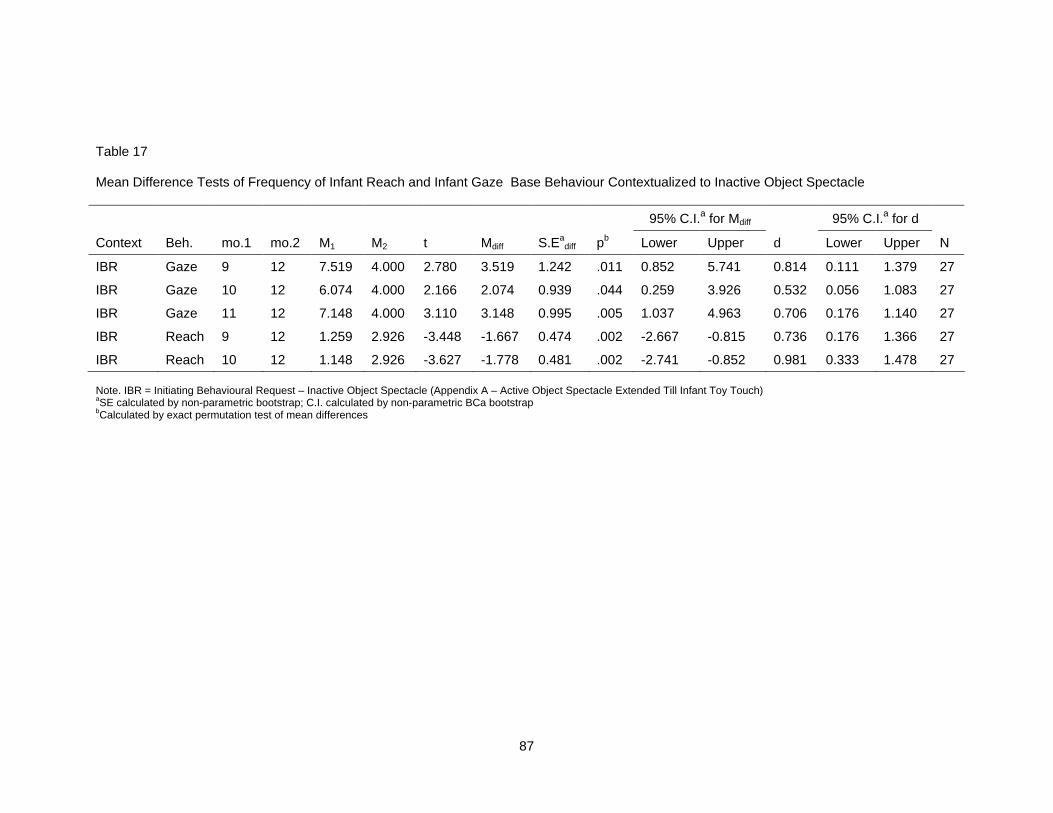
87

Table 17

Mean Difference Tests of Frequency of Infant Reach and Infant Gaze Base Behaviour Contextualized to Inactive Object Spectacle

95% C.I.a for Mdiff 95% C.I.a for d

Context Beh. mo.1 mo.2 M1 M2 t Mdiff S.Eadiff pb Lower Upper d Lower Upper N

IBR Gaze 9 12 7.519 4.000 2.780 3.519 1.242 .011 0.852 5.741 0.814 0.111 1.379 27

IBR Gaze 10 12 6.074 4.000 2.166 2.074 0.939 .044 0.259 3.926 0.532 0.056 1.083 27

IBR Gaze 11 12 7.148 4.000 3.110 3.148 0.995 .005 1.037 4.963 0.706 0.176 1.140 27

IBR Reach 9 12 1.259 2.926 -3.448 -1.667 0.474 .002 -2.667 -0.815 0.736 0.176 1.366 27

IBR Reach 10 12 1.148 2.926 -3.627 -1.778 0.481 .002 -2.741 -0.852 0.981 0.333 1.478 27 Note. IBR = Initiating Behavioural Request – Inactive Object Spectacle (Appendix A – Active Object Spectacle Extended Till Infant Toy Touch) aSE calculated by non-parametric bootstrap; C.I. calculated by non-parametric BCa bootstrap bCalculated by exact permutation test of mean differences

88

IBR Context – Infant Toy Touch

Examination of infant base behaviours that took place while infants manipulated a toy object found that frequencies of Infant Give increased across the assessments (see Table 18). With respect to the developmental stability of infant behaviours, Infant Give displayed stability between 9 and 10 months.

• Context – Infant Toy Touch, Infant Give (9 month / 10 month)

o r(26) = .637, 95% CI [.046, .939], SE = .262, p = .004

Examination of the sequential contingencies of the infant base behaviours with respect to the onset of infants manipulating a toy object found no infant behaviours displayed developmental changes across the assessments. With respect to development stability of sequential infant behaviours contextual to the onset of infants manipulating a toy object no contingent infant behaviours were observed to display developmental stability across the assessments.

Discussion – Initiating Behavioural Response

Considered together, the results suggest the following: Both Higher (Pointing to an inactive toy object; unprompted Giving of toy object to experimenter) and Total IBR composite scores follow the same pattern of developmental change across the assessments. As Higher scores are a component of Total scores, it is reasonable to conclude that the Higher scores constitute the majority of the variance in Total score values. Similarly, the two forms of IBR Give (with and without an Infant Gaze) also follow the same pattern of developmental change, and in turn constitute part of the IBR Higher scores (Gives and Points). Hence, the developmental change observed in infants' IBR behaviours can be accounted for by these two forms of IBR Give behaviour.

With respect to the IBR Lower behaviours of IBR Reach (reaching for an active or inactive toy object without Gazing toward experimenter) and IBR Appeal (reaching for an active or inactive toy object while Gazing toward experimenter), it is interesting that only IBR Appeal underwent a developmental increase in frequency between 10 and 11 months. Additionally, the contingencies for IBR Appeal were observed to undergo developmental changes in frequency. In particular, between 11 and 12 months, the IBR Appeal contingency increased in frequency of first occurrence (i.e., contingent frequency). This suggests that infants are undergoing microgenetic developmental change in the manifestation of their appealing behaviour across the 9-12 month assessments. Moreover, this

89

Table 18

Mean Difference Tests of Infant Give Base Behaviour Contextualized to Infant Toy Touch

95% C.I.a for Mdiff 95% C.I.a for d

Context Beh. mo.1 mo.2 M1 M2 t Mdiff S.Eadiff pb Lower Upper d Lower Upper N

IBR-Toy Give 9 10 0.393 1.214 -3.191 -0.821 0.253 .002 -1.500 -0.429 0.636 0.331 0.956 28

IBR-Toy Give 9 11 0.393 3.000 -4.373 -2.607 0.586 .000 -3.964 -1.607 1.252 0.824 1.731 28

IBR-Toy Give 9 12 0.407 3.778 -5.037 -3.370 0.657 .000 -4.889 -2.259 1.413 0.978 1.899 27

IBR-Toy Give 10 11 1.214 3.000 -2.930 -1.786 0.598 .006 -3.179 -0.786 0.763 0.270 1.216 28

IBR-Toy Give 10 12 1.259 3.778 -3.848 -2.519 0.642 .000 -3.889 -1.370 0.962 0.494 1.396 27 Note. IBR-Toy = Initiating Behavioural Request – Infant Manipulating Toy aSE calculated by non-parametric bootstrap; C.I. calculated by non-parametric BCa bootstrap bCalculated by exact permutation test of mean differences

90

gradual microgenetic development is not detectable by base frequency score measures (i.e., standard ESCS scoring practices).

Another issue is the interactive context that defines the ESCS reaching behaviours. As defined in the ESCS manual, IBR Reach (reaching for a distant toy without gazing toward the experimenter) and IBR Appeal (reaching for a distant toy while gazing toward the experimenter) occur whenever the infant reaches for a toy outside of his or her grasp. This situation arises mainly in two interactive contexts: (a) a toy is active, and (b) a toy is inactive. The ESCS reaching behaviours, therefore, do not discriminate between different manifestations of reaching behaviour in terms of the interactive context of their occurrence. This is understandable given the prevailing functionalist interpretations of joint attention behaviours: infants reach for the toy because they want it, and this “wanting” is independent of the environmental context. However, during the secondary analysis it was found that Infant Reach (when analyzed independent of Infant Gaze) was contingently related to the onset of an active object spectacle, and not to the inactivity of the object. Moreover, with respect to changes in the contextual dependent frequencies of these behaviours, higher instances of change were observed across the assessments in the Active Object Spectacle Event context than in the inactive object spectacle context (Active Object Spectacle Extended Till Infant Toy Touch). This suggests that infants’ manifestations of both IBR Reach and IBR Appeal are situational dependent.

It is noteworthy that although the two IBR Give behaviours (IBR Give With Gaze; IBR Give Without Gaze) are correlated with one another, only one involves the act of Infant Gaze. The question can be raised, therefore, as to the importance of the distinction between the two behaviours. Specifically, if IBR Eye Contact (Gazing toward experimenter while a toy is inactive) had been significantly correlated with IBR Give With Gaze, then the value of the distinction might possibly be suggested. Nevertheless, the IBR Give Without Gaze contingency was observed to undergo developmental change, whereas the IBR Give With Gaze contingency did not. When Infant Give was analyzed in the secondary analysis, independent of Infant Gaze, no developmental changes were observed in the contingencies across the assessments. The lack of developmental change in the [Infant Toy Touch Infant Give] contingency, contrasted with the developmental changes in the IBR Give Without Gaze contingency, suggests that Infant Gaze serves a diagnostic role in differentiating between IBR Give With Gaze and IBR Give Without Gaze behaviours. That is, an Infant Give with an Infant Gaze is not the same thing as an Infant Give without an Infant Gaze, with respect to the consistent behavioural responding of infants.

91

Moreover, standard frequency counts of IBR Give With Gaze were correlated with IJA Alternate (Gazing toward experimenter during active toy object) at 11 and 12 months. These correlations are all the more interesting given the finding that standard frequency counts of IBR Give With Gaze and IBR Give Without Gaze are correlated with one another up to the 11 month assessment; i.e., at the 12 month assessment, these two behaviours are not correlated.

These correlations suggest a possible explanation for the differential developmental of the IBR Give With Gaze and IBR Give Without Gaze contingencies. It may be that, starting around 11 months of age, IBR Give Without Gaze can be classified as an initiating behavioural request behaviour, and that which is known as IBR Give With Gaze might better be classified as an initiating joint attention behaviour (IJA). That is, beginning at 11 months of age infants’ Give With Gaze behaviour in the interactive context of manipulating a toy might be an attempt to share affectivity about the toy by giving the toy to the experimenter. Prior to 11 months of age, however, both forms of IBR Giving behaviours may not be diagnostically distinct with respect to infants’ manifestation of joint attention. Mundy and Gomes (1997) have drawn attention to the possibility that observed correlations among ESCS measures may be specific to particular periods of development (i.e., age specific).

Responding to Behavioural Response

Primary Analysis – Responding to Behavioural Respon se

Infants' RBR behaviours evidenced significant increases in frequency of occurrence in Total Fail and Total Pass frequencies across the months of assessment (see Table 19). Developmental stability was observed for RBR Total Pass between 10 and 12 months, r(25) = .538, 95% CI [.113, .866], SE = .219, p = .005.

Both RBR Pass With Gesture (relinquishing a toy object to the experimenter after she prompts with an open palm gesture) and RBR Pass Without Gesture (relinquishing a toy object to the experimenter after she has made a verbal request for the object) showed increases in frequency across the assessments (see Table 20).

92

Table 19

Mean Difference Tests of RBR Total Fail and RBR Total Pass Standard ESCS Behavioural Frequency Scores

95% C.I.a for Mdiff 95% C.I.a for d

ESCS Behaviour mo.1 mo.2 M1 M2 t Mdiff S.Eadiff pb Lower Upper d Lower Upper N

RBR Total Fail 9 10 2.821 6.536 -2.880 -3.714 1.266 .008 -6.286 -1.321 0.829 0.285 1.420 28

RBR Total Fail 9 11 2.821 7.500 -4.126 -4.679 1.112 .000 -7.107 -2.714 1.140 0.640 1.673 28

RBR Total Fail 9 12 2.926 7.148 -3.778 -4.222 1.097 .001 -6.407 -2.111 1.080 0.513 1.664 27

RBR Total Pass 9 10 0.536 2.714 -3.672 -2.179 0.583 .000 -3.786 -1.321 0.966 0.564 1.340 28

RBR Total Pass 9 11 0.536 5.321 -7.997 -4.786 0.588 .000 -6.214 -3.857 2.037 1.489 2.580 28

RBR Total Pass 9 12 0.556 5.704 -7.339 -5.148 0.689 .000 -6.630 -3.926 2.033 1.387 2.720 27

RBR Total Pass 10 11 2.714 5.321 -3.664 -2.607 0.699 .001 -4.000 -1.250 0.852 0.250 1.366 28

RBR Total Pass 10 12 2.778 5.704 -4.809 -2.926 0.597 .000 -4.074 -1.741 0.910 0.379 1.466 27 Note. RBR = Responding to Behavioural Request aSE calculated by non-parametric bootstrap; C.I. calculated by non-parametric BCa bootstrap bCalculated by exact permutation test of mean differences.

93

Table 20

Mean Difference Tests of RBR Pass With Gesture and RBR Pass Without Gesture Standard ESCS Behavioural Frequency Scores

95% C.I.a for Mdiff 95% C.I.a for d

ESCS Behaviour mo.1 mo.2 M1 M2 t Mdiff S.Eadiff pb Lower Upper d Lower Upper N

RBR Pass c ¯ Gest. 9 10 0.536 2.393 -3.877 -1.857 0.470 .000 -3.000 -1.107 1.004 0.552 1.438 28

RBR Pass c ¯ Gest. 9 11 0.536 4.714 -7.509 -4.179 0.547 .000 -5.536 -3.321 1.901 1.389 2.432 28

RBR Pass c ¯ Gest. 9 12 0.556 4.333 -6.997 -3.778 0.530 .000 -4.889 -2.815 1.852 1.236 2.471 27

RBR Pass c ¯ Gest. 10 11 2.393 4.714 -3.747 -2.321 0.608 .001 -3.679 -1.250 0.877 0.367 1.328 28

RBR Pass c ¯ Gest. 10 12 2.444 4.333 -3.723 -1.889 0.497 .001 -2.778 -0.852 0.748 0.272 1.241 27

RBR Pass s ¯ Gest. 9 10 0.000 0.321 -2.077 -0.321 0.152 .031 -0.929 -0.143 0.565 0.000 0.739 28

RBR Pass s ¯ Gest. 9 11 0.000 0.607 -4.688 -0.607 0.127 .000 -0.929 -0.429 1.276 0.894 1.767 28

RBR Pass s ¯ Gest. 9 12 0.000 1.370 -5.336 -1.370 0.252 .000 -1.963 -0.963 1.480 1.043 1.982 27

RBR Pass s ¯ Gest. 10 12 0.333 1.370 -5.106 -1.037 0.199 .000 -1.481 -0.704 0.950 0.424 1.450 27

RBR Pass s ¯ Gest. 11 12 0.556 1.370 -2.936 -0.815 0.273 .010 -1.407 -0.333 0.793 0.290 1.307 27 Note. RBR = Responding to Behavioural Request; c ¯ = with; s ¯ = without; Gest. = Gesture aSE calculated by non-parametric bootstrap; C.I. calculated by non-parametric BCa bootstrap; bCalculated by exact permutation test of mean differences

94

Comparable to the pattern of correlation between RBR Total Pass, each form of RBR Pass behaviour was correlated with itself between the 10 and 12 month assessments: (a) RBR Pass With Gesture, r(25) = .478, 95% CI [.083, .785], SE = .188, p = .011; (b) RBR Pass Without Gesture, r(25) = .612, 95% CI [.130, .875], SE = .223, p = .003. Moreover, these two RBR passing behaviours were positively correlated with one another at 10 and 12 months.

• RBR Pass With Gesture (10 month) / RBR Pass Without Gesture (10 month)

o r(26) = .703, 95% CI [.230, .919], SE = .218, p = .001

• RBR Pass With Gesture (12 month) / RBR Pass Without Gesture (12 month)

o r(25) = .402, 95% CI [.046, .735], SE = .186, p = .038

For the sequential contingencies of the RBR passing behaviours, only RBR Pass With Gesture displayed developmental change from the 10 to 12 month assessment.

• RBR Pass With Gesture – Contingent Frequency (10 month / 12 month):

o t(14) = -2.667, Mdiff = -1.600, 95% CI [-2.667, -0.400], SE = 0.580, p = .027, d = 0.753, 95% CI [0.061, 1.564]

For the RBR Pass With Gesture sequential contingency, developmental stability was observed in the geometric mean between 11 and 12 months, r(20) = .527, 95% CI [.157, .747], SE = .142, p = .012.

Secondary Analysis – Responding to Behavioural Resp onse

RBR Context – With and Without Gesture

Examination of infant base behaviours that took place during Experimenter Retrieve (experimenter leaning across the table in an attempt to obtain the toy from the infant) found no infant behaviour displayed developmental changes in frequencies across the assessments; similarly, no infant behaviour contextualized to Experimenter Retrieve displayed any developmental stability across the assessments.

Examination of the sequential contingencies of the infant base behaviours with respect to the onset of Experimenter Retrieve found no infant behaviours displayed developmental changes across the assessments. With respect to development stability of sequential infant behaviours contextual to the onset of Experimenter Retrieve no infant behaviours displayed developmental stability across the assessments.

95

GENERAL DISCUSSION

The results of the present study inform the theoretical debates regarding the development of infants’ joint attentional abilities in a number of ways. The results suggest that the manifestations of IJA behaviours (declarative joint attention) are sensitive to interactive context. IJA behaviours of differing contexts are not equivalent in the frequency of their occurrence, or in their inter-relations to one another. This finding runs counter to the established research practice of constructing composite scores by aggregating across individual forms of joint attention behaviour. Specifically, the results of the present study challenge the notion that joint attention behaviours can be neatly categorized according to their morphological complexity (e.g., Lower or Higher behavioural distinction). Issues of behavioural categorization parallel issues regarding context independent definitions of behaviour. The results of the present study suggest that rather than defining joint attention behaviour morphologically, such behaviours may alternatively be defined in terms of situational context. These results are inconsistent with what would be expected from a mentalistic conceptualization of infants’ joint attentional abilities. Specifically, mentalistic accounts would predict a greater degree of homogeneity in infant’s IJA behaviours than was actually observed.

This is most evident in the discussed negative correlations in the secondary analysis between the contingencies of Active Object Spectacle Extended Infant Gaze (IJA Gaze) and Infant Toy Touch Infant Gaze (IJA-Toy Gaze). As mentioned these contingencies involve Infant Gaze, considered independently of any other infant behaviour. That is, with respect to the literature on joint attention, these contingencies are interactively contextualized contingencies of infants’ checking behaviour. As previously discussed, IJA is operationally defined in terms of infants’ “checking” behaviour; i.e., gazing toward the social partner. This behavioural requirement of checking is evidenced in the ESCS by the fact that only one IJA behaviour, Point Without Gaze, does not include a gaze toward the social partner as part of its definition. If the mentalistic conceptualization of joint attention, and its corresponding operational definition/requirement of “checking,” were an accurate model of infant’s joint attentional abilities, then these contingencies would be expected to positively correlated. Specifically, these contingencies represent the central tenet of the mentalistic model of joint attention that underlies all manifestations of

96

joint attention behaviours: “checking” is interpreted as infants ensuring that social partners are paying attention, and hence, this behaviour is taken as supporting evidence that infants understand others as intentional agents. Declarative joint attention (i.e., IJA) can be crudely defined as infant checking plus additional behaviours of varying morphological complexity (e.g., showing, pointing, etc.). The fact that these two contingencies were found to be negatively correlated, an effect in the opposite direction to that predicted by the mentalistic model, suggests that the construct of IJA is too broad as a behavioural class to accurately model infants’ socially interactive behaviours. That is, when IJA behaviours are considered from the perspective of the interactive context of their occurrence, not all IJA behaviours are equivalent (symmetrical). In contrast to the mentalistic conceptualization of infants’ joint attention, a skill-based view of joint attention would expect such asymmetries in infants’ interactive contextual manifestations of joint attention behaviours.

At issue is not whether IJA behaviours should be defined in terms of infants’ gazes toward social partners. Rather, what is at issue is the notion that all IJA behaviours either, (a) result from a unitary development process (e.g., Carpenter et al., 1998; Mundy et al., 2009; Tomasello, 1995); or (b) share functional (operant) equivalency (e.g., Moore & Corkum, 1994) such as providing infants with an affective social reinforcer. What is at issue, therefore, is whether the different forms of IJA behaviours can be classified (composited) as expressions of a single competency, be it cognitive (Carpenter et al., 1998; Tomasello, 1995), neurological (Mundy et al., 2009), or behavioural (Corkum & Moore, 1995; Moore & Corkum, 1994). The results of the present study suggest that such competency models may not fully capture the subtle changes that occur in infants’ development of joint attentional abilities.

Rather, the results of the present study are more in keeping with what would be expected from membership models of development (Chapman, 1987). According to the membership model, infants’ joint attentional abilities are best viewed as existing on a developmental continuum. Joint attention, therefore, need not be conceptualized as being either binary (present/absence) in nature (e.g., Carpenter et al., 1998) or of a consistent (homogenous) kind or type. Instead, joint attentional behaviours can be viewed as sets of independent skills (processes) that may undergo developmental integration and change over time. From this perspective, variations in which individual joint attention behaviours infants engage in at specific points in development ought to be expected; moreover, such behaviours need not be consistently related to one another across all point of development. For example, the finding in the present study that IBR Give With Gaze (unprompted Giving of toy object to experimenter while Gazing toward experimenter) and IJA Alternate (Gazing toward experimenter

97

during active toy object) are correlated during the later assessments suggests that a given skill may serve different functions at different point in development. For any given skill, rather than it being conceived of as arising from a single competency, the competency can be defined in terms of how and when the skill is utilized.

Viewing individual joint attention behaviours as a related set of skills and capacities, rather than as the product of a unitary process, is consistent with a sensorimotor conceptualization of joint attentional abilities. This view of joint attention is supported by the finding that many joint attention behaviours, such as IJA Eye Contact (Gazing toward experimenter while manipulating a toy object) and IJA Show (Gazing toward experimenter and holding up toy object), were contextually, rather than morphologically, related to one another. In contrast, mentalistic conceptualizations of joint attention abstract away from the immediate situational environment in which behaviours occur; i.e., infants’ joint attentional abilities are founded upon a representational capacity. This is an inevitable consequence of viewing joint attention behaviours as communicative signals that infants use to communicate their intent (i.e., cognitive state) to their social partners. Within this view of joint attention the only way that context influences infants’ joint attentional behaviour is if it influences their cognitive states, which in turn, brings about the behaviour. Situational context may moderate infants’ production of joint attentional behaviours, but it is not intrinsic to the production of the behaviour. Sensorimotor schemes, in contrast, are intrinsically contextually dependent, embedded, and embodied (Pfeifer & Bongard, 2007; Pfeifer & Scheier, 1999): “In particular, if the [sensorimotor] model is valid, then all representational phenomena, even, ultimately, formal phenomena, are intrinsically grounded in actual interactions between actual systems and actual environments in real time [italics added], with timing considerations generally playing a critical role” (Bickhard & Terveen, 1995, p. 84).

A central tenet of a skill-based/sensorimotor conceptualization of infants’ joint attentional abilities is the inherent temporality of skills. Several results of the present study illustrate this point. The relation between IJA Eye Contact and IJA Show is a case in point. The straight frequencies of these two behaviours were concurrently positively correlated across the assessments. As discussed, this suggests the sensitivity of behaviour to interactive context. However, these frequency counts do not take the temporality of behaviour into account. In contrast, the analysis of the temporal sequential relations (contingencies) of these two IJA behaviours found them to be negatively correlated, with IJA Eye Contact predicting facets of the IJA Show contingency at the next month. Interpreted differently, the analysis of the straight frequencies can be thought of as establishing the existence of a behavioural relation between these two IJA

98

behaviours. In turn, as the contingency analysis elaborates upon this relation, the two forms of analyses validate one another. However, only the contingency analysis is predictive of later behaviour. This suggests the timing of joint attention behaviours may be of importance in understanding the development of joint attention.

The notion that timing is of importance in understanding the development of skills is further suggested by the observation that for some joint attention behaviours the results of the contingency analysis paralleled that of the frequency analysis. For example, for the IBR Give Without Gaze (unprompted Giving of toy object to experimenter without Gazing toward experimenter) behaviour, the frequency analysis and contingency analysis provide similar results. However, the contingency analysis, as it is based on the timing of events, suggests that changes in the frequency of joint attention behaviours is accompanied by changes in the timing of those behaviours. Necessarily, changes in the timing of behaviours reflect changes in the real-time manifestations of those behaviours. Frequency counts, in contrast, abstract away from performance issues. The fact that results from the analyses of performance correspond with the results of analyses of competency (i.e., frequency counts) suggests that theoretical dissociations between the two may be untenable. In contrast to a mentalistic conceptualization, a skill-based conceptualization of joint attention would expect such parallels between performance and competency as the latter is a conceptual abstraction of the real-time, situational dependent manifestations of skills. Additionally, in the case of IBR Appeal (reaching for an active or inactive toy object while Gazing toward experimenter) behaviour, the contingency analysis revealed developmental changes in the timing of the behaviour during later assessments that were not reflected by corresponding changes in the frequency counts of the behaviour. Changes such as these may be of importance in both understanding and identifying the developmental processes involved in infants’ joint attentional abilities.

The purpose of the present study, as previously stated, was to ascertain whether a skill-based view of joint attention could accumulate sufficient empirical support to justify its pursuit as a viable programme of research. The results of the present study do indeed suggest that such is the case. One of the research goals of the present study was to compare the relative abilities of the standard analysis of the ESCS with an analysis that is consistent with the proposed skill-based framework to detect individual differences in the development of joint attention. The results of the present study suggest a high degree of overlap between the two forms of analyses, as previously discussed. Notwithstanding such congruency, the analysis inspired by a skill-based framework did detect

99

individual difference in the development of joint attention not captured by the standard analysis of the ESCS.

One possible interpretation of the observation that both forms of analysis produced results that were both similar, yet different, is that a great degree of individual variation may exist across infants with respect to their developmental trajectories. The present study, for instance, utilized population/sample level statistics (e.g., mean difference tests) to investigated developmental change. Consequently, an assumption was accepted that all infants in the sample followed the same developmental timetable and trajectory. Typically, research on joint attention tacitly assumes that the development of infants’ joint attentional abilities can be described by a single, universal developmental trajectory. It may be the case that multiple developmental trajectories exist to describe the development of infants’ joint attentional abilities. For example, in the present study a number of significant correlations involved low number of participants (i.e., listwise deletion); the implication of this is that the remaining infants in the sample did not display the behaviour under consideration. Consequently, the microgenetic developmental differences observed in the present study may consist of those developmental patterns that are most common across infants. The use of population/sample level statistics in the present study, therefore, by averaging across the sample, may have prevented the detection of other consistent developmental patterns that were only expressed by sub-groups of infants. The possibility exists, therefore, that different populations of infants may evidence stable and unique differences in the development of joint attentional abilities. Future research can address this issue through a comparative investigation and analysis of multiple case studies examining the development of joint attentional abilities in individuals (cf. Carpendale & Carpendale, 2010; Hendriks-Jansen, 1996). If a single recommendation had to be formulated to guide the development of skill-based research programme, it would be the comparative examination of individual trajectories of development.

The present study suggests a number of research questions to be pursued by future research. The analysis of contingency in the present study only examined the timing between antecedent behaviours or events and the first occurring consequent that followed. It remains to be determined, therefore, how infants’ repetitious use (repairs) of a given behaviour relates to their joint attentional abilities. Alongside repairs, infants’ transitions from one form of joint attention to another during a single joint attentional episode remains to be examined; i.e., interactive repairs that involve different forms of joint attentional behaviours. Such transitions would need to be examined to determine whether or not infants actually engage in such behaviour, and if so, what sequential chains of behaviours are infants observed to consistently perform. For example,

100

if the experimenter does not respond to infants’ initial joint attentional behaviour, how do infants respond? Do they (a) repeat the same behaviour, (b) follow up with a more morphologically complex behaviour, or (c) revert to a preferred behaviour of lower complexity that they made effective use of in prior interactions? Future research is needed to address these questions.

A limitation of the present study is that a limited sample size was utilized. Although the present study attempted to ameliorate this condition through the use of appropriate statistical tests, it is possible that a number of relations among joint attention behaviours were not detected (i.e., Type II error). Future research of this kind would need to employ larger sample sizes. The present study is also limited in that infants were observed/interviewed only once during each assessment month, with the same experimenter. Ideally, infants would be observed multiple times during each assessment month, with these observations being made close in time. Frequent assessments would facilitate analyses in terms of how detected patterns of infant responding developmentally change over time and also increase the reliability of any measures utilized. This would allow for a more accurate assessment of infants’ social understanding. Similarly, multiple assessments could be conducted by different experimenters. The established research practice of using the same experimenter for every assessment, although ensuring measurement reliability, limits information regarding infants’ joint attentional abilities to that observed with only one social partner (Seibert et al., 1987). Multiple assessments by different experimenters would allow for a more global or representative measures of infants’ joint attentional abilities.

Another limitation of the present study is that it focused on infants 9 to 12 months of age. Prior research has established that this is the age range during which joint attention develops. However, little is known of how infants’ experiences at earlier months influence their later development of joint attention. Future research is needed to determine which early developmental factors influence the later development of joint attentional abilities. Similarly, Mundy and Gomes (1997) have discussed the possibility that relations between joint attention variables may change over the course of development. With respect to the present study, further research is needed to determine whether the observed relations between joint attention behaviours change or remain consistent beyond 12 months of age.

Notwithstanding these limitations, the present study does demonstrate that from 9 to 12 months of age infants’ joint attentional abilities undergo microgenetic development. The present study provides numerous illustrations of how standard frequency counts of infants’ joint attentional behaviours fail to

101

adequately capture or reflect such microgenetic changes in development. Such changes may have diagnostic value in the diagnosis and intervention in a number of social communicative disorders, such as autism (e.g., Mundy et al., 2009). Finally, the present study provides a number of novel findings that are of relevance to theoretical debate and discussion regarding the development of infants’ joint attentional abilities. In this respect, two findings are of particular importance. First, infants’ manifested morphologically identical declarative joint attentional behaviours differentially according to interactive context. Second, infants’ joint attentional behaviours that occurred within a particular interactive context were often correlated, despite such behaviours differing substantially in terms of morphological complexity. These findings are inconsistent with mentalistic accounts of joint attention that would expect a greater homogeneity of behaviour across differing interactive contexts than was observed. Therefore, it may be problematic to classify or group some interactive social skills under the category of “joint attention” as somehow being qualitatively distinct from other socially communicative skills. These findings, however, are consistent with a skill-based view of joint attention that views such abilities as developing from out of infants’ relational engagement with their social environments and interactive contexts.

102

REFERENCE LIST

Adamson, L. B., & Bakeman, R. (1984). Mothers' communicative acts: Changes during infancy. Infant Behavior and Development, 7, 467-478.

Allen, J. F. (2001). Bioinformatics and discovery: Induction beckons again. BioEssays, 23, 104-107.

Bakeman, R., & Adamson, L. B. (1984). Coordinating attention to people and objects in mother-infant and peer-infant interaction. Child Development, 55, 1278-1289.

Bakeman R., & Gottman, J. M. (1986). Observing interaction: An introduction to sequential analysis. New York: Cambridge University Press.

Bakeman, R., McArthur, D., Quera, V., & Robinson, B. F. (1997). Detecting sequential patterns and determining their reliability with fallible observers. Psychological Methods, 2(4), 357-370.

Benjamini, Y., Drai, D., Elmer, G., Kafkafi, N., & Golani I. (2001). Controlling the false discovery rate in behavior genetics research. Behavioural Brain Research, 125, 279-284.

Benjamini, Y., & Hochberg, Y. (1995). Controlling the false discovery rate: A practical and powerful approach to multiple testing. Journal of the Royal Statistical Society, Series B, Methodological, 57(1), 289-300.

Benjamini, Y., & Yekutieli, D. (2001). The control of the false discovery rate in multiple testing under dependency. The Annals of Statistics, 29(4), 1165-1188.

Bibok, M. B., Carpendale, J. I. M., & Lewis, C. (2008). Social knowledge as social skill: An action based view of social understanding. In U. Müller, J. I. M. Carpendale, N. Budwig, & B. Sokol (Eds.), Social life and social knowledge: Toward a process account of development (pp. 145-169). Mahwah, NJ: Erlbaum.

Bickhard, M. H., & Terveen, L. (1995). Foundation issues in artificial intelligence and cognitive science: Impasse and solution. Amsterdam: Elsevier.

Blurton Jones, N. (1972). Characteristics of ethological studies of human behaviour. In N. Blurton Jones (Ed.), Ethological studies of child behaviour (pp. 3-33). New York: Cambridge University Press.

103

Bolton, R. J., Hand, D. J., & Adams, N. M. (2002). Determining hit rate in pattern search. In. D. J. Hand, N. M. Adams & R. J. Bolton (Eds.), Pattern detection and discovery, ESF exploratory workshop, London, UK, September 16-19, 2002: proceedings (pp. 36-48). Berlin: Springer.

Brooks, R. A. (1987, September). Planning is just a way of avoiding figuring out what to do next. MIT Artificial Intelligence Laboratory Working Paper 303. Retrieved October 9, 2007, from http://people.csail.mit.edu/brooks/publications.html

Brooks, R. A. (1991a). How to build complete creatures rather than isolated cognitive simulators. In K. Van Lehn (Ed.), Architectures for intelligence (pp. 225-239). Hillsdale, NJ: Erlbaum.

Brooks, R. A. (1991b). Intelligence without representation. Artificial Intelligence, 47, 139-159.

Brooks, R. A. (1995). Intelligence without reason. In L. Steels & R. A. Brooks (Eds.), The artificial life route to artificial intelligence: Building embodied, situated agents (pp. 25-81). Hillsdale, NJ, England: Lawrence Erlbaum Associates, Inc.

Butterworth, G. (1995). Origins of mind in perception and action. In C. Moore, & P. J. Dunham (Eds.), Joint attention: Its origin and role in development (pp. 29-40). Hillsdale, NJ: Lawrence Erlbaum Associates.

Carpendale, J. I. M., & Carpendale, A. B. (2010). The development of pointing: From personal directedness to interpersonal direction. Human Development, 53(3), 110-126.

Carpendale, J. I. M., & Lewis, C. (2004). Constructing an understanding of mind: The development of children’s social understanding within social interaction. Behavioral and Brain Sciences, 27, 79–96.

Carpendale, J. I. M. & Lewis, C. (2006). How children develop social understanding. Oxford: Blackwell.

Carpenter, M., Nagell, K., & Tomasello, M. (1998). Social cognition, joint attention, and communicative competence from 9 to 15 months of age. Monographs of the Society for Research in Child Development, 63(4), (Serial No. 255).

Chapman, M. (1987). Inner processes and outward criteria: Wittgenstein’s importance for psychology. In M. Chapman & R. A. Dixon (Eds.), Meaning and the growth of understanding: Wittgenstein’s significance for developmental psychology (pp. 103–127). Berlin: Springer-Verlag.

Cohen, J. (1960). A coefficient of agreement for nominal scales. Educational and Psychological Measurement, 20(1), 37-46.

Cohen, J. (1992). A power primer. Psychological Bulletin, 112(1), 155-159.

104

Corkum, V., & Moore, C. (1995). Development of joint visual attention in infants. In C. Moore, & P. J. Dunham (Eds.), Joint attention: Its origin and role in development (pp. 61-83). Hillsdale, NJ: Lawrence Erlbaum Associates.

Cumming, G., & Finch, S. (2005). Inference by eye: Confidence intervals and how to read pictures of data. American Psychologist, 60(2), 170-180.

Danziger, K. (1985). The methodological imperative in psychology. Philosophy of the Social Sciences, 15(1), 1-13.

Danziger, K. (1987). Statistical method and the historical development of research practice in American psychology. In L. Krüger, G. Gigerenzer, & M. S. Morgan (Eds.), The probabilistic revolution. Volume 2: Ideas in the sciences (pp. 35-47). Cambridge, MA: MIT Press.

DiCiccio, T. J., & Efron, B. (1996). Bootstrap confidence intervals. Statistical Science, 11(3), 189-228.

Dudley, H., & Ludbrook, J. (1998). Why permutation tests are superior to t and F tests in biomedical research. American Statistician, 52(2), 127-132.

Dunlop, W. P., Cortina, J. M., Vaslow, J. B., & Burke, M. J. (1996). Meta-analysis of experiments with matched groups or repeated measures designs. Psychological Methods, 1(2), 170-177.

Efron, B. (1987). Better bootstrap confidence intervals. Journal of the American Statistical Association, 82(397), 171-185.

Efron, B. (1988). Bootstrap confidence intervals: Good or bad? Psychological Bulletin, 104(2), 293-296.

Ernst, M. D. (2004). Permutation methods: A basis for exact inference. Statistical Science, 19(4), 676-685.

Fischer, K. W. (1980). A theory of cognitive development: The control and construction of hierarchies of skills. Psychological Review, 87(2), 477–531.

Fischer, K. W., & Rose, S. P. (1999). Rulers, clocks, and nonlinear dynamics: Measurement and method in developmental research. In G. Savelsbergh, H. van der Maas, & P. van Geert (Eds.), Nonlinear developmental processes (pp. 197-212). Amsterdam: Royal Netherlands Academy of Arts and Sciences.

Fischer, K. W., Stewart, J., & Stein, Z. (2008). Process and skill: Analyzing dynamic structures of growth. In F. Riffert & H. J. Sander (Eds.), Researching with Whitehead: System and adventure (pp. 327-367). Munich: Verlag Karl Alber.

105

Flynn, E., Pine, K., & Lewis, C. (2007). Using the microgenetic method to investigate cognitive development: An introduction. Infant and Child Development, 16, 1-6.

Frawley, W. J., Piatetsky-Shaprio, G., & Matheus, C. J. (1992). Knowledge discovery in databases: An overview. AI Magazine, 13(3), 57-70.

Glymour, C., Madigan, D., Pregibon, D., & Smyth, P. (1996). Statistical inference and data mining. Communications of the ACM, 39(1), 35-41.

Glymour, C., Madigan, D., Pregibon, D., & Smyth, P. (1997). Statistical themes and lessons for data mining. Data Mining and Knowledge Discovery, 1, 11-28.

Hand, D. J. (1998). Data mining: Statistics and more? The American Statistician, 52(2), 112-118.

Hand, D. J. (1999a). Statistics and data mining: Intersecting disciplines. SIGKDD Explorations, 1(1), 16-19.

Hand, D. J. (1999b). Why data mining is more than statistics writ large. Retrieved February 22, 2010, from http://www.stat.fi/isi99/proceedings/arkisto/varasto/hand0490.pdf

Hand, D. J. (2005). Scientific method and statistics. In. P. Armitage & T. Colton (Eds.), Encyclopedia of Biostatistics. John Wiley & Sons, Ltd.

Hand, D. J., Blunt, G., Kelly, M. G., & Adams, N. M. (2000). Data mining for fun and profit. Statistical Science, 15(2), 111-126.

Hand, D. J., & Bolton, R. J. (2004). Pattern discovery and detection: A unified statistical methodology. Journal of Applied Statistics, 31(8), 885-924.

Hannan, T. E. (1987). A cross-sequential assessment of the occurrences of pointing in 3- to 12-month-old human infants. Infant Behavior and Development, 10, 1l-22.

Hendriks-Jansen, H. (1996). Catching ourselves in the act: Situated activity, interactive emergence, evolution, and human thought. Cambridge: MA, MIT Press.

Hoenig, J. M., & Heisey, D. M. (2001). The abuse of power: The pervasive fallacy of power calculations for data analysis. American Statistician, 55(1), 1-6.

Hubbard, R., & Bayarri, M. J. (2003). P values are not error probabilities. Retrieved January 8, 2010, from http://www.uv.es/sestio/TechRep/tr14-03.pdf

Kahn, W. (2000). Comment – Data Mining for Fun and Profit. Statistical Science, 15(2), 127-130.

106

Kaye, K. (1982). The moral philosophy of microanalysis. In. T. Field & A. Fogel (Eds.), Emotion and early interaction (pp. 237-251). Hillsdale, NJ: Lawrence Erlbaum Associates, Inc.

Legendre, P. (2000). Comparison of permutation methods for the partial correlation and partial mantel tests. Journal of Statistical Computation and Simulation, 67, 37-73.

Leung, E. H. L., & Rheingold, H. L. (1981). Development of pointing as a social gesture. Developmental Psychology, 17(2), 215-220.

Liszkowski, U., Carpenter, M., Henning, A., Striano, T., & Tomasello, M. (2004). Twelve-month-olds point to share attention and interest. Developmental Science, 7(3), 297-307.

Liszkowski, U., Carpenter, M., & Tomasello, M. (2007). Reference and attitude in infant pointing. Journal of Child Language, 34(1), 1-20.

Maass, W. (1997). Networks of spiking neurons: The third generation of neural network models. Neural Networks, 10(9), 1659-1671.

Maass, W., Natschläger, T., & Markram, H. (2002). Real-time computing without stable states: A new framework for neural computation based on perturbations. Neural Computation, 14, 2531-2560.

Magnusson, M. S. (1996). Hidden real-time patterns in intra- and inter-individual behavior: Description and detection. European Journal of Psychological Assessment, 12(2), 112-123.

Magnusson, M. S. (2000). Discovering hidden time patterns in behavior: T-patterns and their detection. Behavior Research Methods, Instruments, & Computers, 32(1), 93-110.

Manly, B. F. J. (1991). Randomization and Monte Carlo methods in biology. New York: Chapman and Hall.

Maturana, H. R., & Varela, F. J. (1987). The tree of knowledge: The biological roots of human understanding. Boston, Massachusetts: Shambhala Publications, Inc.

Matsumoto, M., & Nishimura, T. (1998). Mersenne Twister: A 623-dimensionally equidistributed uniform pseudo-random number generator. ACM Transactions on Modeling and Computer Simulation, 8(1), 3-30.

Messer, D. J., & Vietze, P. M. (1984). Timing and transitions in mother-infant gaze. Infant Behavior & Development, 7, 167-181.

Moore, C. (2007). Show me the theory! British Journal of Developmental Psychology, 25, 39-43.

107

Moore, C., & Corkum, V. (1994). Social understanding at the end of the first year of life. Developmental Review, 14, 349-372.

Morales, M., Mundy, P., Crowson, M. M., Neal, A. R., & Delgado, C. E. F. (2005). Individual differences in infant attention skills, joint attention, and emotion regulation behaviour. International Journal of Behavioral Development, 29(3), 259-263.

Morales, M., Mundy, P., Delgado, C. E. F., Yale, M., Messinger, D., Neal, R., & Schwartz, H. K. (2000). Responding to joint attention across the 6- through 24-month age period and early language acquisition. Journal of Applied Developmental Psychology 21(3), 283–298.

Mundy, P., Block, J., Vaughan Van Hecke, A., Delgado, C., Venezia Parlade, M., & Pomares, Y. (2007). Individual differences and the development of infant joint attention. Child Development, 78, 938–954.

Mundy, P., Delgado, C., Block, J., Venezia, M., Hogan, A., & Seibert, J. (2003). A manual for the abridged early social communication scales (ESCS). Unpublished manuscript, University of Miami, Miami, FL.

Mundy, P., & Gomes, A. (1997). A skills approach to early language development: Lessons from research on developmental disabilities. In L. B. Adamson, & M. A. Romski (Eds.), Communication and language acquisition: Discovers from atypical development (pp. 107-133). Baltimore: Paul H. Brookes Pub.

Mundy, P., & Gomes, A. (1998). Individual differences in joint attention skill development in the second year. Infant Behavior & Development, 21(3), 469-482.

Mundy, P., & Sigman, M. (2006). Joint attention, social competence, and developmental psychopathology. In D. Cicchetti, & D. J. Cohen (Eds.), Developmental psychopathology: Vol. 1. Theory and Method (2nd ed.) (pp. 293-332). Hoboken, NJ: John Wiley & Sons.

Mundy, P., Sullivan, L., & Mastergeorge, A. M. (2009). A parallel and distributed-processing model of joint attention, social cognition and autism. Autism Research, 2, 2-21.

Mundy, P., & Thorp, D. (2006). The neural basis of early joint-attention behavior. In T. Charman, & W. Stone (Eds.), Social and communication development in autism spectrum disorders: Early identification, diagnosis, and intervention (pp. 296-336). New York, NY: Guilford Press.

Parise, E., Cleveland, A., Costabile, A., & Striano, T. (2007). Influence of vocal cues on learning about objects in joint attention contexts. Infant Behavior and Development, 30, 380-384.

108

Parlade, M. V., Messinger, D. S., Delgado, C. E. F., Kaiser, M. Y., Van Hecke, A. V., & Mundy, P. C. (2009). Anticipatory smiling: Linking early affective communication and social outcome. Infant Behavior & Development, 32, 33-43.

Pfeifer, R., & Bongard, J. (2007). How the body shapes the way we think: A new view of intelligence. Cambridge: MA, MIT Press.

Pfeifer, R., & Scheier, C. (1999). Understanding intelligence. Cambridge: MA, MIT Press.

Platt, J. R. (1964). Strong inference. Science, 146, 347-353.

Racine, T. (2005). The role of shared practice in the origins of joint attention and pointing. (Doctoral dissertation, Simon Fraser University, 2005). Dissertation Abstracts International: Section B: The Sciences and Engineering, 67(3-B), 1733.

Racine, T. P., & Carpendale, J. I. M. (2007). The role of shared practice in joint attention. British Journal of Developmental Psychology, 25, 3-25.

Rosnow, R. L., & Rosenthal, R. (1996). Computing contrasts, effect sizes, and counternulls on other people's published data: General procedures for research consumers. Psychological Methods, 1(4), 331-340.

Seibert, J. M., Hogan, A. E., & Mundy, P. C. (1982). Assessing interactional competencies: The Early Social-Communication Scales. Infant Mental Health Journal, 3(4), 244-258.

Seibert, J. M., Hogan, A. E., & Mundy, P. C. (1987). Assessing social and communication skills in infancy. Topics in Early Childhood Special Education, 7(2), 38-48.

Skinner, B. F. (1987). Whatever happened to psychology as the science of behavior? American Psychologist, 42(8), 780-786.

Striano, T., & Rochat, P. (1999). Developmental link between dyadic and triadic social competence in infancy. British Journal of Developmental Psychology, 17, 551-562.

Thelen, E., & Smith, L. B. (1994). A dynamic systems approach to the development of cognition and action. Cambridge: MA, MIT Press.

Thompson, B. (2007). Effect sizes, confidence intervals, and confidence intervals for effect sizes. Psychology in the Schools, 44(5), 423-432.

Tomasello, M. (1995). Joint attention as social cognition. In C. Moore, & P. J. Dunham (Eds.), Joint attention: Its origin and role in development (pp. 103-130). Hillsdale, NJ: Lawrence Erlbaum Associates.

109

Tomasello, M., Carpenter, M., Call, J., Behne, T., & Moll, H. (2005). Understanding and sharing intentions: The origins of cultural cognition. Behavioral and Brain Sciences, 28(5), 675-735.

Tomasello, M., Carpenter, M., & Liszkowski, U. (2007). A new look at infant pointing. Child Development, 78(3), 705-722.

Turnbull, W. (2003). Language in action: Psychological models of conversation. New York: Psychology Press.

Vacha-Haase, T., Nilsson, J. E., Reetz, D. R., Lance, T. S., Thompson, B. (2000). Reporting practices and APA editorial policies regarding statistical significance and effect size. Theory & Psychology, 10(3), 413-425.

van Geert, P. (2003). Dynamic systems approaches and modeling of developmental processes. In J. Valsiner & K. J. Conolly (Eds.), Handbook of Developmental Psychology (pp. 640–672). London: Sage.

van Geert, P., & Fischer, K. W. (2009). Dynamic systems and the quest for individual-based models of change and development. In J. P. Spencer, M. S. C. Thomas, & J. L. McClelland (Eds.), Toward a unified theory of development: Connectionism and dynamic systems theory re-considered (pp. 313-336). New York: Oxford University Press.

Van Hecke, A. V., & Mundy, P. (2007). Neural systems and the development of gaze following and related joint attention skills. In R. Flom, K. Lee, & D. Muir (Eds.), Gaze following: Its development and significance (pp. 17-43). Mahwah, NJ: Lawrence Erlbaum Associates.

Van Hecke, A. V., Mundy, P. C., Acra, C. F., Block, J. J., Delgado, C. E. F., Parlade, M. V.,…Pomares, Y. B. (2007). Infant joint attention, temperament, and social competence in preschool children. Child Development, 78(1), 53-69.

Venezia, M., Messinger, D. S., Thorp, D., & Mundy, P. (2004). The development of anticipatory smiling. Infancy, 6(3), 397-406.

Wilkinson, L., & Task Force on Statistical Inference, American Psychological Association. (1999). Statistical methods in psychology journals: Guidelines and explanations. American Psychologist, 54(8), 597-604.

110

APPENDICES

111

Appendix A: Behavioural Codes

For the following behaviours and events both onsets and offsets were coded. Codes were objectively and physically defined as much as possible. Codes were named with everyday language descriptions (e.g., Infant Reaching) to increase the intelligibility of their labels. However, to avoid ambiguity when explicitly referring to a given code (e.g., Infant Reaching) rather than an ordinary language description (infant reaching) behavioural codes are always capitalized.

Situational Events and Experimenter Behaviours

Active Object Spectacle

Active Object Spectacle refers to an active toy object that is presented to infants. For mechanical wind-up toys, the onset of this event is defined as the first millisecond of audio in which the experimenter begins to wind up a mechanical toy. The offset is defined as the last millisecond of audio in which a mechanical toy still remains active (see Figure 1). For the presentation of the balloon, the onset is defined as the first millisecond of audio that air is released from the inflated balloon; the offset is defined as the last millisecond of audio produced when the balloon contacts the table as experimenter places it on the table surface. For the presentation of the plastic jar, the onset is defined as the first millisecond of audio in which the experimenter begins to shake the jar container; the offset is defined as the last millisecond of audio produced by the jar contacting the table surface as the experimenter placing the jar on the table. For the flower toy, the onset is defined as the first video frame that the experimenter positions the flower stalk in a vertical orientation before commencing to animate the toy; the offset is defined as the last video fame in which the experimenter is still touching the toy after placing it on the table.

Figure 1. Audio waveform of an active mechanical toy (vertical bars denote onset and offset)

112

Active Object Spectacle Extended

Active Object Spectacle Extended is identical to Active Object Spectacle, except that the original offset is extended in time by two seconds (2000 milliseconds). This extension is in accordance with the ESCS manual (Mundy et al., 2003).

Infant Toy Touch

Infant Toy Touch refers to those instances in which infants are actively manipulating/holding a toy. The onset is defined as the first video frame in which the infant makes physical contact with a toy placed before him or her; the offset is defined as the last video frame in which the infant remains in contact with the toy.

Active Object Spectacle Original End Till Infant To y Touch

Active Object Spectacle Original Till Infant Toy Touch refers to the time interval that elapses between an instance of Active Object Spectacle and the first Infant Toy Touch that follows it. The onset is defined as the offset of the Active Object Spectacle; the offset is defined as the onset of the first following Infant Toy Touch. If an Active Object Spectacle is not followed by a corresponding Infant Toy Touch, then the code is not constructed.

Active Object Spectacle Extended Till Infant Toy To uch

Active Object Spectacle Extended Till Infant Toy Touch is constructed much like Active Object Spectacle Original Till Infant Toy Touch except that Active Object Spectacle Extended is used in place of Active Object Spectacle.

Active Object Spectacle Extended Till Infant Toy Touch corresponds to the situational context that defines initiating behavioural requests (IBR) (Mundy et al., 2003).

Viable Object

Viable Object refers to the time interval that elapses between an object spectacle becoming active and the experimenter placing the object on the table in front of an infant. The onset is defined as the onset of an Active Object Spectacle Extended; the offset is defined as the last video frame that the experimenter remains in physical contact with the toy after having placed the toy in front of the infant.

113

Experimenter Still

Experimenter Still refers to those instances in which the experimenter remains still and silent in anticipation of an infant’s joint attentional bids. The onset is defined as the video frame in which the experimenter becomes still after having either manipulated a toy or having placed the toy on the table. The onset is defined as the first video frame in which the experimenter’s hands are either folded in front of her on the table, or when her hands are placed flat on the table. The offset is defined as the first video frame in which the experimenter begins to move her hands or body, thereby breaking from a physically still posture.

Experimenter Talking

Experimenter Talking refers to any utterance made by the experimenter while she was in a state of Experimenter Still. The onset is defined by the first millisecond of audio that the experimenter begins talking; the offset is defined by the last millisecond of audio that the experimenter remains talking, plus an additional second (1000 milliseconds) (see Figure 2).

The function of this code is to mark those time intervals during which an infant’s response toward the experimenter may have been elicited by the experimenter’s talking (Venezia et al., 2004). Together, Experimenter Talking and Experimenter Still serve to filter infants’ social responsive behaviours in order to isolate those behaviours that are not preceded by the experimenter’s talking or moving. Such identified social responsive behaviours, therefore, are considered to be voluntarily initiated by infants, rather than elicited by the experimenter’s behaviour (Mundy et al., 2003). The offset extension (1000 milliseconds) controls for infant responses that occur very shortly after the experimenter has finished talking and therefore are likely to be elicited by the experimenter’s talking.

Figure 2. Audio waveform of experimenter talking (“Wanna see it”) (vertical bars denote onset and offset)

114

Experimenter Palm Up Gesture

Experimenter Palm Up Gesture refers to the gesture that the experimenter uses to signal to an infant that he or she should relinquish possession of a toy over to the experimenter. The gesture is defined as the experimenter having the back of her hand resting on the table surface, palm up, with the fingers of the hand extended. When the experimenter begins to produce this gesture, she will typically move her hand along the table’s surface toward the infant. Initially the little finger of her hand will be resting upon the table surface, with the thumb of the hand pointing toward the ceiling. As she moves her hand near the infant, her hand rolls outward to expose the palm of her hand. Ultimately, the hand can rotate no further, at which point the experimenter has fully assumed the gesture.

The onset is defined as the first video frame in which the experimenter has rotated her hand outward to a 45 degree angle, relative to the surface of the table. The offset is defined as either (a) the first video frame that the experimenter grasps the toy object if offered by the infant, (b) the first video frame in which the experimenter begins to fold/curl her fingers to cover her exposed palm, or (c) the video frame in which the experimenter has rolled her hand back inward to a 45 degree, relative to the surface of the table (typically occurs when reaching to take a toy object from an uncooperative infant). Experimenter Palm Up Gesture is identical to the requesting gesture outlined in the ESCS manual used for evaluating infants’ ability to respond to behavioural requests (RBR) (Mundy et al., 2003).

Verbal Command

Verbal Command refers to utterances by the experimenter that are instructions (commands) directed toward the infant when requesting that the infant give the experimenter back a toy object. Examples include, “Give it to me” and “Can I have it?” The onset is defined as the first millisecond of audio that the utterance begins; the offset is defined as the last millisecond of the utterance (see Figure 3). Verbal Command is identical to the command utterance outlined in the ESCS manual used for evaluating infants’ ability to respond to behavioural requests (RBR) (Mundy et al., 2003).

115

Figure 3. Audio waveform of verbal command (“Can I have it?”) (vertical bars denote onset and offset)

Experimenter Retrieve

Experimenter Retrieve refers to the time interval in which the experimenter moves toward the infant to request a toy object in the infant’s possession until the experimenter has obtained possession of the toy. The onset is defined as the first video frame in which the experimenter breaks from Experimenter Still and beings moving toward the infant to retrieve the toy. The offset is defined as the video frame in which the experimenter successfully secures the toy from the infant. Conversely, the offset is also defined as the last video frame that the infant is still in physical contact with the toy before the experimenter comes to be in possession of the toy.

Experimenter Retrieve With Gesture

Experimenter Retrieve With Gesture refers to an instance of Experimenter Retrieve in which the experimenter also performs the Experimenter Palm Up Gesture. That is, the onset and offset are identical to that of the Experimenter Retrieve during which the Experimenter Palm Up Gesture occurs. Experimenter Retrieve With Gesture, therefore, is a type or secondary coding of Experimenter Retrieve. This code is not mutually exclusive with Experimenter Retrieve, so an interval of time can be coded as both Experimenter Retrieve and Experimenter Retrieve With Gesture. This code establishes the contextual preconditions to determine whether infants can successfully respond to behavioural requests (RBR) done through gestures as defined in the ESCS manual (Mundy et al., 2003).

Experimenter Retrieve Without Gesture

Experimenter Retrieve Without Gesture is constructed much like Experimenter Retrieve With Gesture, except that instead of the experimenter performing an Experimenter Palm Up Gesture she performs a Verbal Command instead.

116

Following the ESCS manual, the experimenter was instructed to either request an object by using a Verbal Command or an Experimenter Palm Up Gesture, but not both. Hence, Experimenter Retrieve With Gesture and Experimenter Retrieve Without Gesture are by definition mutually exclusive. However, neither is mutually exclusive with Experimenter Retrieve.

Experimenter Retract

Experimenter Retract refers to the interval of time during which the experimenter has retrieved a toy object from an infant and is in the process of returning the toy to her side of the table. The onset is defined as the first video frame in which the experimenter begins to move away from an infant after having secured a toy object from the infant. The offset is defined as the video frame in which either (a) the experimenter’s body is vertically aligned over her chair, or (b) the experimenter has brought the toy back to a position directly in front of her (in instances in which the experimenter does not need to leave her seat to request the toy from the infant).

Infant Behaviours

Infant Gaze

Infant Gaze refers to those instances that infants look directly toward the upper portion of the experimenter’s face (i.e., the experimenter’s eyes). The onset is defined as the first video frame that the infant looks toward the experimenter’s face; the offset is defined as the last video frame in which the infant remains looking toward the experimenter’s face.

Infant Give

Infant Give refers to those instances in which an infant either (a) hands the experimenter a toy, or (b) offers the experimenter a toy by pushing it toward her or holding it out toward the experimenter with an outstretched arm. The onset is defined as the first video frame that the infant begins to move a toy toward the experimenter so as to either, (a) hold it out toward the experimenter so that she may retrieve it, or (b) place the toy in the experimenter’s open palm (Experimenter Palm Up Gesture). The offset is defined as the video frame in which the infant ceases to touch or be in physical contact with the toy. This will occur for one of two reasons: (a) the experimenter has taken possession of the toy, or (b) the infant will no longer be in contact with the toy after having pushed it toward the experimenter. If during the offer phase of the give (i.e., outstretched

117

arm) the infant brings the toy back toward him or herself, the infant’s behaviour is coded as an Infant Show instead of an Infant Give (Mundy et al., 2003).

Infant Show

Infant Show refers to those instances in which an infant holds a toy upward toward the experimenter’s face while the infant gazes (Infant Gaze) toward the experimenter’s face. The Infant Gaze does not need to occur through out the course of the showing of the toy, but must occur at some point during the episode. The toy must be held relatively motionless in the air for approximately two seconds (Mundy et al., 2003). The onset is defined as the first video frame in which the infant begins to move the toy upward toward the experimenter’s face. The offset is defined as the video frame in which the infant either (a) begins to lower the toy after it has remained motionless, or (b) breaks eye contact with the experimenter (Infant Gaze offset).

Infant Point

Infant Point refers to those instances in which an infant points toward an out of reach toy. The onset is defined as the first video frame in which the infant begins to move his or her hand toward an out of reach toy in what will ultimately culminate in a pointing gesture: extended index finger directed toward the toy with the remaining fingers of the hand either curled against the palm, or bent so as to be orthogonal to the extended index finger. The offset is defined as the video frame that the infant ceases extending his or her index finger toward the out of reach toy.

Infant Reach

Infant Reach refers to all those instances in which infants reach toward a toy that is not within their grasp. The onset is defined as the first video frame in which the infant begins to move his or her hand toward an out of reach toy with all the fingers of the outstretched hand extended toward the toy. The offset is defined as the video frame in which the infant ceases extending her hand toward the toy (i.e., the infant either begins to retract her hand, or curls her fingers into the palm of her hand).

As per the ESCS manual, Infant Reaches that occur within two seconds (2000 milliseconds) of one another are concatenated as a single instance of Infant Reach: the onset is defined as the onset of the first occurring Infant Reach, and the offset is defined as the offset of the second occurring Infant Reach.

118

Infant Composite / Overlapping Behavioural Codes

Still Codes

The following codes are identical to the previously defined infant codes, except that their onset must occur during Experimenter Still and must not occur during an Experimenter Talking. That is, they are a secondary coding of the previously defined codes. As such, they are not mutually exclusive with the previously outlined infant codes. Codes are labeled as follows: the base infant code name is given first in the name and the suffix “Still” is added to the base code name.

The following Still codes were derived: (a) Infant Gaze Still, (b) Infant Give Still, (c) Infant Show Still, (d) Infant Point Still, and (e) Infant Reach Still.

Overlapping Codes

The following codes are created through combinations of the previously defined infant codes. The base (constituent) codes involved, therefore, will not be defined; only the formulas of their combinations will be given. These overlap codes were created in order to allow for the construction of the standard ESCS behavioural codes (procedure defined in next section below) (see, Mundy et al., 2003).

Gaze With Point

Consists of the overlapping video frames in which (a) Infant Gaze and (b) Infant Point co-occur. These overlapping video frames must beginning in a time interval defined by (c) Experimenter Still.

Gaze With Point Retract

Consists of the overlapping video frames in which (a) Infant Gaze and (b) Infant Point co-occur. These overlapping video frames must beginning in a time interval defined by (c) Experimenter Retract.

Gaze Without Point

Consists of instances of (a) Infant Gaze that do not overlap at any point in time (i.e., any video frames) with instances of (b) Infant Point. The Infant Gaze must begin in a time interval defined by Experimenter Still.

119

Gaze Without Point Retract

Consists of instances of (a) Infant Gaze that do not overlap at any point in time (i.e., any video frames) with instances of (b) Infant Point. The Infant Gaze must begin in a time interval defined by Experimenter Retract.

Give With Gaze

Consists of the overlapping video frames in which (a) Infant Gaze and (b) Infant Give co-occur. These overlapping video frames must beginning in a time interval defined by (c) Experimenter Still.

Give Without Gaze

Consists of instances of (a) Infant Give that do not overlap at any point in time (i.e., any video frames) with instances of (b) Infant Gaze. The Infant Give must begin in a time interval defined by Experimenter Still.

Point With Gaze

Consists of the overlapping video frames in which (a) Infant Point and (b) Infant Gaze co-occur. These overlapping video frames must beginning in a time interval defined by (c) Experimenter Still.

Point With Gaze Retract

Consists of the overlapping video frames in which (a) Infant Point and (b) Infant Gaze co-occur. These overlapping video frames must beginning in a time interval defined by (c) Experimenter Retract.

Point Without Gaze

Consists of instances of (a) Infant Point that do not overlap at any point in time (i.e., any video frames) with instances of (b) Infant Gaze. The Infant Point must begin in a time interval defined by Experimenter Still.

Point Without Gaze Retract

Consists of instances of (a) Infant Point that do not overlap at any point in time (i.e., any video frames) with instances of (b) Infant Gaze. The Infant Point must begin in a time interval defined by Experimenter Retract.

120

Reach With Gaze

Consists of the overlapping video frames in which (a) Infant Reach and (b) Infant Gaze co-occur. These overlapping video frames must beginning in a time interval defined by (c) Experimenter Still.

Reach With Gaze Retract

Consists of the overlapping video frames in which (a) Infant Reach and (b) Infant Gaze co-occur. These overlapping video frames must beginning in a time interval defined by (c) Experimenter Retract.

Reach Without Gaze

Consists of instances of (a) Infant Reach that do not overlap at any point in time (i.e., any video frames) with instances of (b) Infant Gaze. The Infant Reach must begin in a time interval defined by Experimenter Still.

Reach Without Gaze Retract

Consists of instances of (a) Infant Reach that do not overlap at any point in time (i.e., any video frames) with instances of (b) Infant Gaze. The Infant Reach must begin in a time interval defined by Experimenter Retract.

ESCS Composite Codes

The following are compositional definitions of the behavioural codes that appear in the ESCS manual (Mundy et al., 2003) in terms of the previously defined overlap codes. As per the ESCS manual, the following codes were created to be mutually exclusive. That is, if an instance of given behaviour is involved in the construction of one ESCS code it cannot be involved in the construction of other ESCS codes. For example, if an Infant Gaze is involved in the construction of an IJA Eye Contact episode, that same Infant Gaze cannot be involved in the construction of an IJA Point With Gaze Higher. Necessarily, the ESCS codes were constructed in order from highest to lowest behavioural complexity to ensure the mutually exclusivity condition.

121

Initiating Joint Attention

IJA Point Without Gaze Higher

Defined as instances of Point Without Gaze that occur within a time interval defined by Active Object Spectacle Extended.

IJA Point With Gaze Higher

Defined as instances of Point With Gaze that occur within a time interval defined by Active Object Spectacle Extended.

IJA Show Higher

Defined as instances of Infant Show that occur within a time interval defined by Experimenter Still.

IJA Eye Contact Lower

Defined as instances of Infant Gaze that occur within a time interval defined by Infant Toy Touch, and which are mutually exclusive (not involved in) with instances of IJA Show Higher.

IJA Eye Alternate Lower

Defined as instances of Gaze Without Point (i.e., mutually exclusivity condition) that occur within a time interval defined by Active Object Spectacle Extended.

IJA Frequency Higher Level

Defined as any instance of the following: (a) IJA Point Without Gaze Higher, (b) IJA Point With Gaze Higher, or (c) IJA Show Higher.

IJA Frequency Lower Level

Defined as any instance of the following: (a) IJA Eye Contact Lower, or (b) IJA Eye Alternate Lower.

122

IJA Frequency Total

Defined as any instance of the following: (a) IJA Frequency Higher Level, or (b) IJA Frequency Lower Level.

Initiating Behavioural Request

IBR Reach Lower

Defined as instances of Reach Without Gaze (i.e., mutually exclusivity condition) that occur within a time interval defined by Viable Object.

IBR Reach Retract Lower

Defined as instances of Reach Without Gaze Retract (i.e., mutually exclusivity condition) that occur within a time interval defined by Experimenter Retract.

IBR Appeal Lower

Defined as instances of Reach With Gaze (i.e., mutually exclusivity condition) that occur within a time interval defined by Viable Object.

IBR Appeal Retract Lower

Defined as instances of Reach With Gaze Retract (i.e., mutually exclusivity condition) that occur within a time interval defined by Experimenter Retract.

IBR Give Without Gaze Higher

Defined as instances of Give Without Gaze (i.e., mutually exclusivity condition) that occur within a time interval defined by Infant Toy Touch.

IBR Give With Gaze Higher

Defined as instances of Give With Gaze (i.e., mutually exclusivity condition) that occur within a time interval defined by Infant Toy Touch.

123

IBR Point Without Gaze Higher

Defined as instances of Point Without Gaze (i.e., mutually exclusivity condition) that occur within a time interval defined by Active Object Spectacle Extended Till Infant Toy Touch.

IBR Point Without Gaze Retract Higher

Defined as instances of Point Without Gaze Retract (i.e., mutually exclusivity condition) that occur within a time interval defined by Experimenter Retract.

IBR Point With Gaze Higher

Defined as instances of Point With Gaze (i.e., mutually exclusivity condition) that occur within a time interval defined by Active Object Spectacle Extended Till Infant Toy Touch.

IBR Point With Gaze Retract Higher

Defined as instances of Point With Gaze Retract (i.e., mutually exclusivity condition) that occur within a time interval defined by Experimenter Retract.

IBR Eye Contact Lower

Defined as instances of Infant Gaze that occur within a time interval defined by Active Object Spectacle Extended Till Infant Toy Touch, and which are mutually exclusive with (a) IBR Point With Gaze Higher, (b) IBR Appeal Lower, and (c) IBR Give With Gaze Higher.

IBR Eye Contact Retract Lower

Defined as instances of Infant Gaze that occur within a time interval defined by Experimenter Retract, and which are mutually exclusive with (a) IBR Point With Gaze Retract Higher, and (b) IBR Appeal Retract Lower.

IBR Frequency Higher Level

Defined as any instance of the following: (a) IBR Give Without Gaze Higher, (b) IBR Give With Gaze Higher, (c) IBR Point Without Gaze Higher, (d) IBR Point With Gaze Higher, (e) IBR Point Without Gaze Retract Higher, or (f) IBR Point With Gaze Retract Higher

124

IBR Frequency Lower Level

Defined as any instance of the following: (a) IBR Reach Lower, (b) IBR Appeal Lower, (c) IBR Eye Contact Lower, (d) IBR Reach Retract Lower, (e) IBR Appeal Retract Lower, or (f) IBR Eye Contact Retract Lower.

IBR Frequency Total

Defined as any instance of the following: (a) IBR Frequency Higher Level, or (b) IBR Frequency Lower Level.

Responding to Behaviour Request

RBR Pass Without Gesture

Defined as instances of Infant Give that occur within a time interval defined by Experimenter Retrieve Without Gesture.

RBR Fail Without Gesture

Defined as instances of Experimenter Retrieve Without Gesture that do not overlap at any point (video frames) with Infant Give.

RBR Pass With Gesture

Defined as instances of Infant Give that occur within a time interval defined by Experimenter Retrieve With Gesture.

RBR Fail With Gesture

Defined as instances of Experimenter Retrieve With Gesture that do not overlap at any point (video frames) with Infant Give.

RBR Total Pass

Defined as instances of the following: (a) RBR Pass Without Gesture, or (b) RBR Pass With Gesture.

RBR Total Fail

Defined as instances of the following: (a) RBR Fail Without Gesture, or (b) RBR Fail With Gesture.

125

Appendix B: Description of Monte Carlo Procedure

The statistical analysis of contingent sequential relations utilized in the current study is based in large part on the inspiration (though not the methodology) underlying the work of Magnusson (1996, 2000). Specifically, Magnuson proposed a method for the empirical detection of temporal sequential relations in behavioural data streams. A behavioural data stream is defined as an ordered sequential list of behaviours or events whose start and stop times are time coded using a metric of discrete units (e.g., milliseconds, seconds, video frames). Typically, a behavioural data stream consists of multiple behaviours whose start and stop times are measured relative to a known reference time point, usually the first instance that observations of behaviour are recorded (time = 0 seconds, 0 video frames, etc.). Temporal sequential relations express the likelihood that given the occurrence of an antecedent behaviour that a specific consequent behaviour will follow it in time after a specific interval of time (delay) has elapsed. Temporal sequential relations of behaviours can be thought of as behavioural patterns with consistent timing. Magnusson's approach to the empirical detection of temporal sequential relations relies upon determining potential durations for the time intervals between the onsets of discrete behavioural events based upon the observed temporal separations between the events in a given behavioural data stream. These potential durations (time intervals or time windows) are then tested to determine if they describe the observed temporal distributions of antecedent and consequent behaviours in the data stream at a level above chance. Such temporal sequential relations, therefore, consist of behaviours that repeat in the “same order each time” throughout a behavioural data stream, and whose temporal separation remains “relatively invariant” with respect to a null hypothesis that no such temporal invariance holds between the behaviours (Magnusson, 2000, p. 94). Such empirical detection of temporal sequential relations, therefore, can be regarded as a method of knowledge discovery: “the nontrivial extraction of implicit, previously unknown, and potentially useful information from data” (Frawley, Piatetsky-Shaprio, & Matheus, 1992).

To illustrate, consider the following behavioural data stream:

A, B, E, C, Z, A, D, E, C, A, F, G, C.

Given this behavioural data stream, a sequential relation between A and C can be observed: C occurs, invariantly, in the third position after A. Such a temporally invariant sequential relation holds even if other behavioural codes (letters, in this example) occur between the two codes. Magnusson has referred to such temporal sequential relations as “hidden behavior patterns” because the

126

sequential relations detected between any two behavioural codes can be detected even if other intervening behavioural codes occur between the two codes being analyzed. Such intervening codes can make such patterns difficult to detect for an unaided observer (Magnusson, 1996). Moreover, as such detection is empirically driven (more on this later) it requires no a priori specification of the anticipated lag (delay) between the codes; “Between the components of a [sequential pattern], the number and type of behaviors that may occur may vary greatly from instance to instance of the same pattern, which makes the detection of such patterns difficult with methods that depend only on the order or sequence of events” (Magnusson, 2000, p. 94). This is in contrast to traditional event-based sequential analysis (Bakeman & Gottman, 1986).

Magnusson has referred to the empirically detected sequential patterns as T-patterns (temporal patterns). The detection algorithm functions by examining both the sequential order of behavioural codes, and the invariant timing between those codes. This represents an additional and substantial advantage over traditional methods of sequential analysis (specifically, event-based sequential analysis). In event-based sequential analysis, behavioural events are coded according to a system of mutually exclusive and exhaustive behavioural codes (e.g., Bakeman & Adamson, 1984). These events are without duration; hence, the sequential nature of a behavioural data stream is describable only in terms of before and after. As such, all repeating pairs of codes (e.g., A, B) in the data stream are statistically treated as equivalent, even though the temporal delay between the codes may vary widely. Such forms of sequential analysis, therefore, place artificial constraints upon the behavioural data stream in order that it may be statistically analyzed thereby, "forc[ing] the phenomenon into something it is not" (Magnusson, 1996, p. 116). Additionally, the statistics used to determine the measure of association (contingency) between two behavioural codes (e.g., Yule’s-Q, log-odds ratio) require that the behavioural codes used be mutually exclusive and exhaustive. In contrast, the empirical detection of sequential patterns proposed by Magnusson places no such temporal constraints on the behavioural data stream, nor necessitates the use of mutually exclusive and exhaustive behavioural codes. This is advantageous, as according to Magnusson (2000, p. 94), “[with respect to the phenomenon under investigation,] analysis using this method is objective and operationalized, so it requires no prior commitment to a particular theoretical viewpoint [as to how the phenomenon should unfold over time]” (see Danziger, 1985, 1987, for an in-depth treatment of the relation between psychological theory and statistics).

127

Monte Carlo (Method of Statistical Trials)

To determine whether significant temporal sequential relations hold between behavioural codes, the following approach will be utilized.

The total observational period is divided into a number discrete time units of equal duration, henceforth referred to as NT: the total duration of the behavioural data stream. For example, a one minute observational period can be thought of as being composed of 60 discrete seconds; hence, if the unit of time in which behaviours are recorded is seconds, then NT = 60.

The occurrence of a behavioural code is defined by its onset (and additionally the offset if desired) in terms of the discrete unit of time used. For example, using seconds as the unit of time, with NT = 60 seconds, the onset of a behavioural code could occur at 5, 9, 45, or 59 seconds, but not 5.5 seconds. That is, each of a code’s “occurrences [are] located in time but may be considered as being without duration” (Magnusson, 1996, p. 116). Given the assumption that one code (henceforth referred to as code A) is associated with the occurrence of a following code (henceforth referred to as code B), the question is whether the probability of the occurrence of code B some time after an occurrence of code A is given by chance (i.e., a random occurrence). That is, are the temporal occurrences of B’s in the data stream conditional on the temporal occurrence of the A’s?

To assess this relation it is necessary that the temporal occurrence (position) of A’s in the data stream be held constant. The temporal sequential relation between A and B can thereafter be stated as follows:

Holding the total number of A’s observed (NA) over the observational period constant at the temporal position of their observed occurrence, what is the probability that the total number of B’s observed (NB) over the observational period occur at the temporal position of their observed occurrence, such that the temporal distances (separations) between non-repeating A’s and the first B codes that follow them occurs by chance?

Non-repeating means that only A’s whose next following code (in terms of codes A and B under consideration – any number of irrelevant codes, such as C, D, or E, can readily occur) is not another A, but instead a B (Magnusson, 2000). This definition holds even if more than two behavioural codes comprise the data stream, as the sequential relation analyzed is only between two codes at any given time. Thus, if a repeating sequence of A’s occurs in the data stream, followed by a repeating sequence of B’s (e.g., A, A, A, C, C, B, B) only the

128

temporal distance between the last A in the sequence and the first following B are considered (positions 3 and 6, respectively).

The reason why only non-repeating A’s are examined is as follows. If repeating A’s are considered it would be necessary to state that the following B is conditional on each preceding A, each considered independently of the other A’s. As there would be no way to decide with which A to pair the B, it would necessary to enumerate multiple separations, one for each pairing. This would have the effect of biasing the detection of temporal sequential relations. In effect, it would reduce the probability that such separations could occur by chance, as the enumerated separations would be very close to one another in terms of temporal distance. This is especially so if the repeating A’s are grouped together very in close in time. These two reasons are also applicable to the stipulation that temporal sequential relations only involve the first B following the last repeating A. The stipulation of only examining non-repeating A’s and first following B’s is considered a “conservative” approach to addressing the difficulties raised by the occurrences of repeating A’s and B’s (Magnusson, 2000, p. 108).

The following example is illustrative. Suppose five A’s are observed over, NT = 60 seconds, at times 2, 13, 24, 35, and 46, and that five B’s are observed over NT at times 7, 18, 29, 40, and 56. In this scenario, the temporal distances between the A’s and their respectively following B’s are 5 and 10 seconds. These temporal distances are empirically given by the data set (e.g., 7 seconds – 2 seconds = 5 seconds, etc.). These temporal distances (time windows) are referred to as fast intervals: no B can happen too fast after the occurrence of an A (see Figure 4) (Magnusson, 2000). These fast intervals are then fitted back to the behavioural data stream to determine the number of times that any non-repeating A will be followed by a B within each of the computed intervals. With a fast interval of 5 seconds, four B’s are observed to occur within an interval of 5 seconds after the occurrence of a preceding, non-repeating A and the next occurrence of an A in the data stream. With a fast interval of 10 seconds, five B’s are observed to occur within an interval of 10 seconds after the occurrence of a preceding, non-repeating A and the next occurrence of an A in the data stream.

129

Figure 4. Example of fast intervals (topmost connectors) and free intervals (bottommost connectors) between two codes on a discrete interval time-line (Magnusson, 2000, p. 97)

Given these two fast intervals (5 and 10 seconds), the following statistical questions can be asked: what is the probability that any given B in the data stream will occur such that its occurrence will fall within (a) a time interval defined by the onset of a preceding A and the onset of that A plus 5 seconds; or (b) a time interval defined by the onset of a preceding A and the onset of that A plus 10 seconds? For example, given the A’s in the behavioural data stream, what is the probability of the B’s occurring in the follow time intervals by chance: (a) 2 – 7, 13 – 18, 24 – 29, 35 – 40, and 46 – 51; or (b) 2 – 12, 13 – 23, 24 – 34, 35 – 45, and 46 – 56? This question is repeated for each fast interval computed (in this example, there are only two fast intervals).

To determine this probability, the following approach is taken. In this example, there are two fast intervals whose probabilities are to be assessed: five seconds (with a total of four B’s occurring within the interval) and 10 seconds (with a total of five B’s occurring within the interval). First, holding the temporal occurrences of the A’s constant (NA), randomly generate the onsets of five B events (i.e., NB) such that (a) their values range from 1 – NT, (b) the probability of the occurrence of each value over the range of 1 – NT is uniformly distributed (i.e., equal probability), and (c) that no randomly generated B event has the same value as any other previously generated B event or A event to ensure that the total of randomly generated B events equal NB. Next, determine (a) the number of first occurring, randomly generated B’s that occur within 5 seconds of the onset of a preceding, non-repeating A, and (b) the number of first occurring randomly generated B’s that occur within 10 seconds of the onset of a preceding, non-repeating A. Compare these values to the number of B’s that were empirically observed to occur within the two computed fast intervals; i.e., 4 and 5, respectively. For each respective fast interval, if the number of randomly generated B’s occurring within the fast interval is equal to or greater than the number of B’s empirically occurring within the fast interval then record a tally (i.e., record a value of one) for that specific fast interval. An occurrence of an equal or greater number of randomly generated B’s occurring in a given fast interval than the number of observed empirical B’s occurring in the same fast interval indicates that the possibility that the number of empirical B’s occurring in the fast interval

130

could have randomly occurred by chance. Next, repeat this process over a number of trials (also known as experiments). Finally divide the number of tallies for each fast interval by the number of trials. The resulting percentages will approximate the probabilities of the B’s in the data stream occurring after an occurrence of an A within each respective fast interval by chance. At 40,000 trials, the observed probabilities will be accurate within ± 0.005%.

In the preceding example, only two fast intervals were observed in the data stream. However, the B’s in a real behavioural data stream never follow the A’s as perfectly as in this example. The maximum number of observable fast intervals that can occur in any behavioural data stream is a function of NA and NB. If NA is equal to or greater than NB, then the maximum possible number of fast intervals is NB (if NB is equal to or greater than NA, then the reverse relation holds). Regardless of the number of fast intervals, the preceding Monte Carlo procedure remains the same.

With two or more fast intervals, it is also possible to compute what is referred to as a free interval (Magnusson, 2000). Unlike the fast interval, which always begins immediately after the onset of an A code, the free interval allows the start of the time interval to freely vary after the onset of an A code. That is, the free interval allows for a delay between the onset of an A code and the start of the time interval. The set of possible start and stop times for the free interval are determined from the computed fast intervals. For example, suppose three fast intervals: 0-5, 0-10, and 0-15 seconds. By computing all order preserving binary permutations (i.e., the stop time can never exceed the start time) of these three time intervals, the following free intervals are produced: 5-10 seconds, 5-15 seconds, and 10-15 seconds. The free intervals represent the succeeding temporal differences between shorter fast intervals and longer fast intervals. Unlike the fast interval, the free interval captures the idea that a B code may follow after an A code after a given delay. The free-interval captures the temporal grouping of B’s within the fast intervals, and therefore provides more information regarding the sequential relation between A and B than the fast interval. In Figure 1 the topmost lines connecting A and B represent fast intervals.

The method and logic of the calculation of the probability associated with each free interval is identical to that of the previously discussed Monte Carlo method: (a) determine the number of first occurring B’s in the data stream that follow within each free interval relative to a preceding, non-repeating occurrence of A; (b) randomly generate NB uniformly distributed events over 1 – NT, in accordance with the previously specified restrictions; (c) count the number of randomly generated first occurring B events falling within each free interval that

131

follows a preceding, non-repeating A event; (d) record the number of occurrences in which the count obtained from step (c) equals or exceeds the number of empirical B events occurring within each free interval in the behavioural data stream; and (e) divide the cumulative count produced by step (d) by the number of trials to determine the probability of the observed free intervals occurring by chance.

Preference for Free Intervals

The procedure outlined above will result in the construction of both fast and free intervals for any given pair of codes. There exists a certain degree of redundancy between the fast interval and the free interval, as the fast intervals are used to construct the free intervals. However, both do not describe the exact same sequential relation, as the free interval permits a delay between an A code and the following B code to occur. Consequently, to maintain consistency in the description of the sequential relations among a set of codes, only one type of time interval should be reported. Between the two types of intervals, the current study exclusively uses the free interval.

Free Interval Selection

In the current study, the above procedure was run using 1,000,000 trials for all possible, two-code, sequential relations between behavioural codes. For each temporal tested sequential relation, one free interval was selected to be representative of the sequential relation. Two goals in the selection process were that (a) the probability associated with the free interval be less than or equal to .05, and (b) the selected free interval would have the greatest number of consequent events (B codes in the previous discussion) associated with it than any of the other free intervals with a probability equal to or less than .05. Consequently, the free interval selected can be interpreted as the free interval that significantly described, to the greatest degree possible (most frequently occurring), the temporal sequential relation under analysis. In the event that no free interval could be found that was less than or equal to .05, then it was assumed that the temporal sequential relation under investigation did not occur with sufficient consistency to be a meaningful aspect in that particular infant’s behavioural repertoire. Consequently, all descriptive statistical measures (more below) for that tested temporal sequential relation, for that particular infant, were set to null values (i.e., missing values).

An intended consequence of the above selection criteria is that it serves as a means of outlier detection. That is, any B codes that do not occur within the selected free interval can be considered to be outliers. This is in contrast to the

132

majority of infant behavioural studies (e.g., Carpenter et al., 1998; Mundy et al., 2003) that treat all infant behaviours as of equal relevance. Understandably, the notion of an infant behaviour occurring by chance is questionable – “Did the infant gaze at the experimenter by accident or for no reason at all (i.e., random occurrence).” The role of the free interval selected, therefore, is not to claim that consequent behaviours (B code) occurring outside of it occur by chance. Instead, it is to claim that those behaviours are rare, atypical occurrences, and represent a lack of behavioural coordination on the part of the infant with respect to his or her environment. Lack of behavioural coordination, however, can refer equally well to either (a) a lack of behavioural coordination and integration, or (b) a developmental cusp in which behavioural coordination becomes less stable just prior to reintegration at a higher level of behavioural skill or ability (Fischer et al., 2008). Regardless, the notion underlying the selection of a significant free interval is to capture the notion of developmental stability in behaviour instead of developmental fluctuations. Unless variability due to developmental stability and developmental fluctuation are analyzed separately, it is very likely that the two sources of variability will tend to cancel one another out during data analysis. That is, unlike the frequency counts utilized in the majority of developmental studies (Mundy et al., 2003; Venezia et al., 2004; Parlade et al., 2009, etc.), the free interval represents a variable range of stable behavioural responsiveness (cf. Fischer & Rose, 1999; Fischer et al., 2008; van Geert, 2003; van Geert & Fischer, 2009).

Once a free interval was selected in accordance with the above stipulations, a number of descriptive measures were calculated to describe the free interval (sequential relation). However, if no free interval was selected, the following descriptive measures simply took on null values (i.e., undefined, missing values, not zero as that value is meaningful). First, the frequency of first occurring consequent behaviours that fall within the free interval after a non-repeating antecedent behaviour can be tallied. This will henceforth be referred to as Monte Frequency. Additionally, the latencies (time elapsed between the antecedent and the consequent) of these first occurring consequent behaviours can be noted. Dispersion (variability) is a useful statistical description of the consistency of a given behaviour. The current study used the absolute mean deviation of these noted latencies as such a measure of behavioural consistency; henceforth, referred to as Monte Latency Dispersion. The absolute mean deviation was selected in place of the standard deviation as the latter is heavily biased when used to describe the dispersion of non-normal distributions. Finally, using the selected free interval, it is possible to compute a measure of association (contingency scores) between the two behavioural codes. To achieve such a measure of association it is possible to compute the geometric

133

mean (also referred to as the limit of phi) of (a) the conditional probability of a B code occurring within the selected time interval after an A code, and (b) the conditional probability that an A code will not be followed by a B code that occurs within the selected time interval after the A code (in accordance with the previously specified restrictions on non-repeating A values and first occurring B values). Henceforth, this measure of association will be referred to as Monte Geometric Mean.

The data analytic procedure previously described was implemented as a C++ program written by myself. The pseudorandom number generator utilized was the Mersenne Twister (Matsumoto & Nishimura, 1998).

134

Appendix C: Descriptive Statistics

Table C1

Descriptive Statistics of Standard ESCS Behavioural Frequency Scores

95% C.I.a for Mean

ESCS Behaviour mo. Mean SD SE a Min Max N Lower Upper

IJA Lower

Eye Cont. 9 6.679 8.870 1.646 0 26 28 3.786 10.321

10 9.250 10.504 1.950 0 39 28 5.893 13.643

11 6.929 7.897 1.465 0 26 28 4.321 10.071

12 4.889 8.030 1.515 0 25 27 2.407 8.481

Eye Alt. 9 0.786 3.315 0.615 0 17 28 0.000 2.786

10 0.536 1.732 0.321 0 8 28 0.107 1.500

11 2.750 5.147 0.954 0 17 28 1.250 5.179

12 3.778 5.846 1.104 0 19 27 2.000 6.444

IJA Lower Freq. 9 7.464 9.754 1.811 0 30 28 4.321 11.500

10 9.786 10.720 1.990 0 39 28 6.321 14.214

11 9.679 10.224 1.898 0 32 28 6.250 13.714

12 8.667 11.526 2.178 0 42 27 5.185 14.037

IJA Higher

Pt. c ¯ Gaze 9 0.000 0.000 0.000 0 0 28 0.000 0.000

10 0.107 0.416 0.077 0 2 28 0.000 0.321

11 0.321 0.863 0.160 0 4 28 0.071 0.786

12 0.815 3.000 0.567 0 15 27 0.111 3.037

Pt. s ¯ Gaze 9 0.000 0.000 0.000 0 0 28 0.000 0.000

10 0.750 2.319 0.431 0 9 28 0.143 1.964

11 0.393 1.197 0.222 0 6 28 0.107 1.179

12 0.852 1.703 0.322 0 6 27 0.333 1.630

Show 9 0.964 1.478 0.274 0 5 28 0.500 1.607

10 1.214 1.315 0.244 0 5 28 0.750 1.714

11 2.036 3.271 0.608 0 16 28 1.179 3.893

12 0.667 1.209 0.228 0 4 27 0.296 1.222

IJA Higher Freq. 9 0.964 1.478 0.274 0 5 28 0.500 1.607

10 2.071 3.355 0.622 0 13 28 1.143 3.714

11 2.750 3.903 0.725 0 17 28 1.643 4.643

135

95% C.I.a for Mean

ESCS Behaviour mo. Mean SD SE a Min Max N Lower Upper

12 2.333 4.279 0.808 0 19 27 1.185 4.704

IJA Tot. Freq. 9 8.429 10.942 2.032 0 32 28 4.893 12.929

10 11.857 12.669 2.350 0 40 28 7.679 16.964

11 12.429 13.500 2.507 0 46 28 8.000 17.893

12 11.000 13.000 2.453 0 45 27 6.889 16.741

IBR Lower

Eye Cont. 9 0.000 0.000 0.000 0 0 28 0.000 0.000

10 0.000 0.000 0.000 0 0 28 0.000 0.000

11 0.000 0.000 0.000 0 0 28 0.000 0.000

12 0.222 1.155 0.218 0 6 27 0.000 0.667

Eye Cont. Ret. 9 0.000 0.000 0.000 0 0 28 0.000 0.000

10 0.000 0.000 0.000 0 0 28 0.000 0.000

11 0.000 0.000 0.000 0 0 28 0.000 0.000

12 0.000 0.000 0.000 0 0 27 0.000 0.000

Reach 9 0.214 0.418 0.077 0 1 28 0.071 0.357

10 0.071 0.262 0.049 0 1 28 0.000 0.179

11 0.143 0.356 0.066 0 1 28 0.036 0.250

12 0.333 0.679 0.128 0 3 27 0.111 0.667

Reach Ret. 9 0.036 0.189 0.035 0 1 28 0.000 0.107

10 0.000 0.000 0.000 0 0 28 0.000 0.000

11 0.036 0.189 0.035 0 1 28 0.000 0.107

12 0.000 0.000 0.000 0 0 27 0.000 0.000

Appeal 9 5.607 7.969 1.480 0 26 28 3.143 9.071

10 5.321 6.504 1.207 0 22 28 3.321 8.214

11 9.357 9.056 1.683 0 30 28 6.286 12.893

12 7.370 7.401 1.398 0 25 27 4.963 10.519

Appeal Ret. 9 1.000 1.925 0.357 0 7 28 0.429 1.857

10 0.964 1.598 0.296 0 6 28 0.464 1.679

11 1.571 1.913 0.355 0 7 28 0.964 2.357

12 1.222 1.672 0.316 0 6 27 0.667 1.926

IBR Lower Freq. 9 6.857 9.272 1.720 0 31 28 4.000 10.893

10 6.357 7.304 1.354 0 25 28 4.107 9.536

11 11.107 10.315 1.915 0 33 28 7.607 15.107

136

95% C.I.a for Mean

ESCS Behaviour mo. Mean SD SE a Min Max N Lower Upper

12 9.148 8.347 1.576 0 31 27 6.444 12.704

IBR Higher

Give c ¯ Gaze 9 0.214 0.499 0.093 0 2 28 0.071 0.429

10 0.429 0.742 0.138 0 2 28 0.179 0.714

11 1.036 1.261 0.234 0 5 28 0.607 1.536

12 1.852 2.699 0.510 0 13 27 1.111 3.370

Give s ¯ Gaze 9 0.714 1.084 0.201 0 4 28 0.357 1.143

10 2.964 3.144 0.583 0 13 28 2.000 4.357

11 6.357 5.071 0.941 0 22 28 4.786 8.571

12 6.370 4.143 0.782 0 16 27 4.926 8.000

Pt. c ¯ Gaze 9 0.000 0.000 0.000 0 0 28 0.000 0.000

10 0.000 0.000 0.000 0 0 28 0.000 0.000

11 0.000 0.000 0.000 0 0 28 0.000 0.000

12 0.074 0.267 0.050 0 1 27 0.000 0.185

Pt. s ¯ Gaze 9 0.000 0.000 0.000 0 0 28 0.000 0.000

10 0.143 0.448 0.083 0 2 28 0.000 0.357

11 0.143 0.448 0.083 0 2 28 0.000 0.357

12 0.148 0.456 0.086 0 2 27 0.000 0.370

Pt. c ¯ Gaze Ret. 9 0.000 0.000 0.000 0 0 28 0.000 0.000

10 0.000 0.000 0.000 0 0 28 0.000 0.000

11 0.000 0.000 0.000 0 0 28 0.000 0.000

12 0.000 0.000 0.000 0 0 27 0.000 0.000

Pt. s ¯ Gaze Ret. 9 0.000 0.000 0.000 0 0 28 0.000 0.000

10 0.107 0.567 0.105 0 3 28 0.000 0.321

11 0.036 0.189 0.035 0 1 28 0.000 0.107

12 0.000 0.000 0.000 0 0 27 0.000 0.000

IBR Higher Freq. 9 0.929 1.152 0.214 0 4 28 0.536 1.357

10 3.643 3.744 0.695 0 13 28 2.464 5.214

11 7.571 5.959 1.107 0 26 28 5.714 10.143

12 8.444 5.169 0.977 1 20 27 6.667 10.519

IBR Tot. Freq. 9 7.786 9.215 1.709 0 31 28 4.929 11.750

10 10.000 8.861 1.646 0 28 28 7.071 13.571

11 18.679 13.870 2.570 2 54 28 14.143 24.321

137

95% C.I.a for Mean

ESCS Behaviour mo. Mean SD SE a Min Max N Lower Upper

12 17.593 11.666 2.203 1 48 27 13.630 22.333

RBR

Fail c ¯ Gest. 9 2.571 3.011 0.559 0 9 28 1.536 3.750

10 5.679 4.643 0.861 0 14 28 4.000 7.393

11 5.857 3.960 0.735 0 14 28 4.464 7.321

12 5.704 3.770 0.712 1 12 27 4.333 7.111

Fail s ¯ Gest. 9 0.250 0.585 0.109 0 2 28 0.071 0.500

10 0.857 1.079 0.200 0 3 28 0.464 1.250

11 1.643 1.339 0.249 0 5 28 1.143 2.143

12 1.444 1.251 0.236 0 5 27 1.000 1.926

Pass c ¯ Gest. 9 0.536 1.138 0.211 0 4 28 0.214 1.071

10 2.393 2.409 0.447 0 10 28 1.607 3.393

11 4.714 2.955 0.548 0 14 28 3.750 5.929

12 4.333 2.703 0.510 0 10 27 3.296 5.333

Pass s ¯ Gest. 9 0.000 0.000 0.000 0 0 28 0.000 0.000

10 0.321 0.819 0.152 0 4 28 0.107 0.786

11 0.607 0.685 0.127 0 2 28 0.357 0.857

12 1.370 1.334 0.252 0 5 27 0.889 1.889

RBR Tot. Fail 9 2.821 3.367 0.625 0 11 28 1.679 4.143

10 6.536 5.501 1.021 0 17 28 4.571 8.571

11 7.500 4.857 0.901 0 18 28 5.786 9.321

12 7.148 4.504 0.850 1 17 27 5.556 8.889

RBR Tot. Pass 9 0.536 1.138 0.211 0 4 28 0.214 1.071

10 2.714 3.041 0.565 0 14 28 1.821 4.179

11 5.321 3.186 0.591 0 15 28 4.286 6.643

12 5.704 3.462 0.654 0 15 27 4.444 7.037 Note. IJA = Initiating Joint Attention; IBR = Initiating Behavioural Request; RBR = Responding to Behavioural Request; c ¯ = with; s ¯ = without; Disp. = Dispersion; Geo. = Geometric Mean; Freq. = Contingent Frequency; Ret. = Retract; Pt. = Point; Gest. = Gesture; Cont. = Contact; Alt. = Alternate aSE calculated by non-parametric bootstrap; C.I. calculated by non-parametric BCa bootstrap

138

Table C2

Descriptive Statistics for ESCS Behavioural Contingencies

95% C.I.a for Mean

ESCS Code mo. M SD SE a Min Max N Lower Upper

IJA Lower

Eye Alt.

Freq. 9 8.50 4.95 2.47 5.00 12.00 2 5.00 8.50

Freq. 10 3.67 1.53 0.72 2.00 5.00 3 2.00 4.67

Freq. 11 7.00 5.07 1.77 2.00 13.00 7 3.71 10.57

Freq. 12 8.00 6.22 1.96 2.00 18.00 9 4.56 12.22

Geo. 9 0.30 0.03 0.01 0.28 0.31 2 0.28 0.30

Geo. 10 0.11 0.01 0.00 0.11 0.12 3 0.11 0.12

Geo. 11 0.21 0.16 0.05 0.03 0.45 7 0.12 0.33

Geo. 12 0.27 0.18 0.06 0.03 0.46 9 0.15 0.36

Disp. 9 1648.72 1570.56 785.31 538.17 2759.28 2 538.17 1648.72

Disp. 10 1616.19 1544.70 728.63 518.08 3382.50 3 518.08 2571.00

Disp. 11 2240.62 1720.82 602.22 156.50 4965.89 7 1174.89 3530.13

Disp. 12 1341.50 1323.45 415.82 181.00 4500.89 9 769.69 2613.66

Eye Cont.

Freq. 9 9.91 4.66 1.34 4.00 18.00 11 7.27 12.45

Freq. 10 9.63 6.08 1.47 2.00 18.00 16 6.63 12.38

Freq. 11 7.60 5.69 1.42 2.00 18.00 15 5.07 10.67

Freq. 12 9.22 5.14 1.62 3.00 17.00 9 6.00 12.33

139

95% C.I.a for Mean

ESCS Code mo. M SD SE a Min Max N Lower Upper

Geo. 9 0.33 0.16 0.04 0.09 0.52 11 0.23 0.41

Geo. 10 0.27 0.19 0.05 0.03 0.59 16 0.18 0.36

Geo. 11 0.20 0.16 0.04 0.00 0.46 15 0.13 0.28

Geo. 12 0.29 0.16 0.05 0.07 0.50 9 0.19 0.39

Disp. 9 2353.48 1140.02 327.31 447.75 4075.14 11 1670.16 2955.30

Disp. 10 1301.64 1092.11 264.67 24.00 4290.31 16 869.90 1940.74

Disp. 11 970.25 861.00 214.77 62.00 2567.25 15 591.11 1436.88

Disp. 12 1237.47 954.41 299.70 172.00 2702.96 9 717.83 1901.30

IJA Higher

Pt. c ¯ Gaze

Freq. 9 0.00 0.00 0.00 0.00 0.00 0 0.00 0.00

Freq. 10 2.00 0.00 0.00 0.00 0.00 1 0.00 0.00

Freq. 11 3.00 1.41 0.71 2.00 4.00 2 2.00 3.00

Freq. 12 6.50 3.54 1.77 4.00 9.00 2 4.00 6.50

Geo. 9 0.00 0.00 0.00 0.00 0.00 0 0.00 0.00

Geo. 10 0.15 0.00 0.00 0.00 0.00 1 0.00 0.00

Geo. 11 0.24 0.13 0.06 0.14 0.33 2 0.14 0.24

Geo. 12 0.40 0.02 0.01 0.39 0.41 2 0.39 0.40

Disp. 9 0.00 0.00 0.00 0.00 0.00 0 0.00 0.00

Disp. 10 1574.00 0.00 0.00 0.00 0.00 1 0.00 0.00

Disp. 11 1413.94 1028.75 514.27 686.50 2141.38 2 686.50 1413.94

Disp. 12 1915.59 582.71 291.25 1503.56 2327.63 2 1503.56 1915.59

140

95% C.I.a for Mean

ESCS Code mo. M SD SE a Min Max N Lower Upper

Pt. s ¯ Gaze

Freq. 9 0.00 0.00 0.00 0.00 0.00 0 0.00 0.00

Freq. 10 6.67 2.31 1.09 4.00 8.00 3 4.00 8.00

Freq. 11 4.00 2.83 1.41 2.00 6.00 2 2.00 4.00

Freq. 12 3.17 1.47 0.55 2.00 6.00 6 2.33 4.50

Geo. 9 0.00 0.00 0.00 0.00 0.00 0 0.00 0.00

Geo. 10 0.47 0.18 0.09 0.34 0.68 3 0.34 0.58

Geo. 11 0.24 0.23 0.12 0.08 0.40 2 0.08 0.24

Geo. 12 0.21 0.14 0.05 0.11 0.48 6 0.14 0.37

Disp. 9 0.00 0.00 0.00 0.00 0.00 0 0.00 0.00

Disp. 10 2523.04 1296.70 611.33 1207.13 3799.63 3 1207.13 3387.21

Disp. 11 1330.75 1234.25 617.60 458.00 2203.50 2 458.00 1330.75

Disp. 12 959.52 703.92 262.61 52.00 1882.00 6 450.74 1468.30

Show

Freq. 9 3.17 1.47 0.55 2.00 5.00 6 2.17 4.17

Freq. 10 2.78 0.97 0.31 2.00 5.00 9 2.22 3.44

Freq. 11 4.18 3.82 1.10 2.00 15.00 11 2.73 7.82

Freq. 12 3.00 0.82 0.35 2.00 4.00 4 2.00 3.50

Geo. 9 0.20 0.09 0.03 0.13 0.34 6 0.15 0.29

Geo. 10 0.20 0.09 0.03 0.10 0.40 9 0.16 0.27

Geo. 11 0.24 0.16 0.04 0.08 0.57 11 0.17 0.35

Geo. 12 0.17 0.04 0.02 0.12 0.22 4 0.13 0.20

141

95% C.I.a for Mean

ESCS Code mo. M SD SE a Min Max N Lower Upper

Disp. 9 1710.34 1226.57 456.39 4.50 3087.52 6 717.84 2524.50

Disp. 10 1796.53 2285.30 718.59 156.50 7327.50 9 835.15 4080.88

Disp. 11 1393.32 1007.69 289.68 106.00 3593.33 11 923.52 2092.94

Disp. 12 2230.99 610.58 264.46 1432.89 2920.00 4 1641.10 2602.77

IBR Lower

Appeal

Freq. 9 8.33 4.42 1.22 2.00 14.00 12 5.67 10.50

Freq. 10 6.29 4.90 1.15 2.00 16.00 17 4.29 8.88

Freq. 11 9.83 4.26 0.98 2.00 16.00 18 7.72 11.56

Freq. 12 7.26 4.82 1.08 2.00 19.00 19 5.42 9.68

Geo. 9 0.35 0.16 0.05 0.07 0.55 12 0.25 0.43

Geo. 10 0.29 0.19 0.05 0.05 0.60 17 0.20 0.38

Geo. 11 0.40 0.14 0.03 0.10 0.71 18 0.34 0.46

Geo. 12 0.37 0.17 0.04 0.06 0.58 19 0.29 0.43

Disp. 9 2592.38 1564.24 431.96 650.00 5566.95 12 1814.48 3513.76

Disp. 10 1743.79 1255.08 295.43 141.00 4520.45 17 1225.52 2394.87

Disp. 11 2451.70 1035.25 236.81 694.44 4000.33 18 1993.14 2921.11

Disp. 12 1656.21 1054.78 235.48 85.00 3990.32 19 1221.57 2146.58

Appeal Ret.

Freq. 9 4.40 1.82 0.73 2.00 7.00 5 2.80 5.60

Freq. 10 3.50 1.38 0.51 2.00 6.00 6 2.67 4.67

Freq. 11 3.45 1.63 0.47 2.00 7.00 11 2.64 4.45

142

95% C.I.a for Mean

ESCS Code mo. M SD SE a Min Max N Lower Upper

Freq. 12 3.11 1.17 0.37 2.00 5.00 9 2.33 3.78

Geo. 9 0.00 0.00 0.00 0.00 0.00 5 0.00 0.00

Geo. 10 0.00 0.00 0.00 0.00 0.00 6 0.00 0.00

Geo. 11 0.00 0.00 0.00 0.00 0.00 11 0.00 0.00

Geo. 12 0.00 0.00 0.00 0.00 0.00 9 0.00 0.00

Disp. 9 361.54 192.67 77.02 193.50 676.41 5 246.26 565.54

Disp. 10 348.24 301.48 112.32 36.44 886.00 6 175.64 634.58

Disp. 11 246.17 180.11 51.78 34.89 664.25 11 166.98 381.14

Disp. 12 272.13 209.91 65.99 42.50 590.56 9 154.17 413.01

Eye Cont.

Freq. 9 0.00 0.00 0.00 0.00 0.00 0 0.00 0.00

Freq. 10 0.00 0.00 0.00 0.00 0.00 0 0.00 0.00

Freq. 11 0.00 0.00 0.00 0.00 0.00 0 0.00 0.00

Freq. 12 0.00 0.00 0.00 0.00 0.00 0 0.00 0.00

Geo. 9 0.00 0.00 0.00 0.00 0.00 0 0.00 0.00

Geo. 10 0.00 0.00 0.00 0.00 0.00 0 0.00 0.00

Geo. 11 0.00 0.00 0.00 0.00 0.00 0 0.00 0.00

Geo. 12 0.00 0.00 0.00 0.00 0.00 0 0.00 0.00

Disp. 9 0.00 0.00 0.00 0.00 0.00 0 0.00 0.00

Disp. 10 0.00 0.00 0.00 0.00 0.00 0 0.00 0.00

Disp. 11 0.00 0.00 0.00 0.00 0.00 0 0.00 0.00

Disp. 12 0.00 0.00 0.00 0.00 0.00 0 0.00 0.00

143

95% C.I.a for Mean

ESCS Code mo. M SD SE a Min Max N Lower Upper

Eye Cont. Ret.

Freq. 9 0.00 0.00 0.00 0.00 0.00 0 0.00 0.00

Freq. 10 0.00 0.00 0.00 0.00 0.00 0 0.00 0.00

Freq. 11 0.00 0.00 0.00 0.00 0.00 0 0.00 0.00

Freq. 12 0.00 0.00 0.00 0.00 0.00 0 0.00 0.00

Geo. 9 0.00 0.00 0.00 0.00 0.00 0 0.00 0.00

Geo. 10 0.00 0.00 0.00 0.00 0.00 0 0.00 0.00

Geo. 11 0.00 0.00 0.00 0.00 0.00 0 0.00 0.00

Geo. 12 0.00 0.00 0.00 0.00 0.00 0 0.00 0.00

Disp. 9 0.00 0.00 0.00 0.00 0.00 0 0.00 0.00

Disp. 10 0.00 0.00 0.00 0.00 0.00 0 0.00 0.00

Disp. 11 0.00 0.00 0.00 0.00 0.00 0 0.00 0.00

Disp. 12 0.00 0.00 0.00 0.00 0.00 0 0.00 0.00

Reach

Freq. 9 0.00 0.00 0.00 0.00 0.00 0 0.00 0.00

Freq. 10 0.00 0.00 0.00 0.00 0.00 0 0.00 0.00

Freq. 11 0.00 0.00 0.00 0.00 0.00 0 0.00 0.00

Freq. 12 0.00 0.00 0.00 0.00 0.00 0 0.00 0.00

Geo. 9 0.00 0.00 0.00 0.00 0.00 0 0.00 0.00

Geo. 10 0.00 0.00 0.00 0.00 0.00 0 0.00 0.00

Geo. 11 0.00 0.00 0.00 0.00 0.00 0 0.00 0.00

Geo. 12 0.00 0.00 0.00 0.00 0.00 0 0.00 0.00

144

95% C.I.a for Mean

ESCS Code mo. M SD SE a Min Max N Lower Upper

Disp. 9 0.00 0.00 0.00 0.00 0.00 0 0.00 0.00

Disp. 10 0.00 0.00 0.00 0.00 0.00 0 0.00 0.00

Disp. 11 0.00 0.00 0.00 0.00 0.00 0 0.00 0.00

Disp. 12 0.00 0.00 0.00 0.00 0.00 0 0.00 0.00

Reach Ret.

Freq. 9 0.00 0.00 0.00 0.00 0.00 0 0.00 0.00

Freq. 10 0.00 0.00 0.00 0.00 0.00 0 0.00 0.00

Freq. 11 0.00 0.00 0.00 0.00 0.00 0 0.00 0.00

Freq. 12 0.00 0.00 0.00 0.00 0.00 0 0.00 0.00

Geo. 9 0.00 0.00 0.00 0.00 0.00 0 0.00 0.00

Geo. 10 0.00 0.00 0.00 0.00 0.00 0 0.00 0.00

Geo. 11 0.00 0.00 0.00 0.00 0.00 0 0.00 0.00

Geo. 12 0.00 0.00 0.00 0.00 0.00 0 0.00 0.00

Disp. 9 0.00 0.00 0.00 0.00 0.00 0 0.00 0.00

Disp. 10 0.00 0.00 0.00 0.00 0.00 0 0.00 0.00

Disp. 11 0.00 0.00 0.00 0.00 0.00 0 0.00 0.00

Disp. 12 0.00 0.00 0.00 0.00 0.00 0 0.00 0.00

IBR Higher

Give c ¯ Gaze

Freq. 9 2.00 0.00 0.00 0.00 0.00 1 0.00 0.00

Freq. 10 2.00 0.00 0.00 2.00 2.00 4 2.00 2.00

Freq. 11 2.56 1.01 0.32 2.00 5.00 9 2.11 3.33

145

95% C.I.a for Mean

ESCS Code mo. M SD SE a Min Max N Lower Upper

Freq. 12 4.00 2.98 0.89 2.00 12.00 10 2.80 6.90

Geo. 9 0.14 0.00 0.00 0.00 0.00 1 0.00 0.00

Geo. 10 0.17 0.07 0.03 0.11 0.27 4 0.12 0.24

Geo. 11 0.15 0.08 0.03 0.00 0.30 9 0.10 0.21

Geo. 12 0.26 0.14 0.04 0.11 0.56 10 0.20 0.36

Disp. 9 4597.00 0.00 0.00 0.00 0.00 1 0.00 0.00

Disp. 10 2008.88 2382.68 1032.00 133.00 5150.50 4 158.50 3908.88

Disp. 11 1618.79 1292.56 406.31 88.00 3255.36 9 829.74 2414.66

Disp. 12 2218.11 1753.87 525.18 217.50 5364.50 10 1369.05 3492.87

Give s ¯ Gaze

Freq. 9 2.50 0.84 0.31 2.00 4.00 6 2.00 3.17

Freq. 10 4.41 2.74 0.65 2.00 11.00 17 3.35 6.00

Freq. 11 6.84 4.90 0.96 2.00 21.00 25 5.24 9.12

Freq. 12 7.62 3.61 0.77 2.00 15.00 21 6.19 9.24

Geo. 9 0.21 0.09 0.03 0.10 0.35 6 0.15 0.28

Geo. 10 0.30 0.17 0.04 0.00 0.62 17 0.22 0.38

Geo. 11 0.43 0.21 0.04 0.09 0.76 25 0.36 0.52

Geo. 12 0.50 0.21 0.04 0.04 0.82 21 0.41 0.58

Disp. 9 3431.25 1567.92 584.45 1812.50 5287.00 6 2330.71 4676.75

Disp. 10 2930.78 2376.11 558.92 165.50 8168.96 17 1983.33 4208.76

Disp. 11 3162.30 1697.98 332.77 438.89 6451.30 25 2525.73 3826.38

Disp. 12 3238.72 1416.66 301.56 1.50 5545.00 21 2602.25 3788.68

146

95% C.I.a for Mean

ESCS Code mo. M SD SE a Min Max N Lower Upper

Pt. c ¯ Gaze

Freq. 9 0.00 0.00 0.00 0.00 0.00 0 0.00 0.00

Freq. 10 0.00 0.00 0.00 0.00 0.00 0 0.00 0.00

Freq. 11 0.00 0.00 0.00 0.00 0.00 0 0.00 0.00

Freq. 12 0.00 0.00 0.00 0.00 0.00 0 0.00 0.00

Geo. 9 0.00 0.00 0.00 0.00 0.00 0 0.00 0.00

Geo. 10 0.00 0.00 0.00 0.00 0.00 0 0.00 0.00

Geo. 11 0.00 0.00 0.00 0.00 0.00 0 0.00 0.00

Geo. 12 0.00 0.00 0.00 0.00 0.00 0 0.00 0.00

Disp. 9 0.00 0.00 0.00 0.00 0.00 0 0.00 0.00

Disp. 10 0.00 0.00 0.00 0.00 0.00 0 0.00 0.00

Disp. 11 0.00 0.00 0.00 0.00 0.00 0 0.00 0.00

Disp. 12 0.00 0.00 0.00 0.00 0.00 0 0.00 0.00

Pt. c ¯ Gaze Ret.

Freq. 9 0.00 0.00 0.00 0.00 0.00 0 0.00 0.00

Freq. 10 0.00 0.00 0.00 0.00 0.00 0 0.00 0.00

Freq. 11 0.00 0.00 0.00 0.00 0.00 0 0.00 0.00

Freq. 12 0.00 0.00 0.00 0.00 0.00 0 0.00 0.00

Geo. 9 0.00 0.00 0.00 0.00 0.00 0 0.00 0.00

Geo. 10 0.00 0.00 0.00 0.00 0.00 0 0.00 0.00

Geo. 11 0.00 0.00 0.00 0.00 0.00 0 0.00 0.00

Geo. 12 0.00 0.00 0.00 0.00 0.00 0 0.00 0.00

147

95% C.I.a for Mean

ESCS Code mo. M SD SE a Min Max N Lower Upper

Disp. 9 0.00 0.00 0.00 0.00 0.00 0 0.00 0.00

Disp. 10 0.00 0.00 0.00 0.00 0.00 0 0.00 0.00

Disp. 11 0.00 0.00 0.00 0.00 0.00 0 0.00 0.00

Disp. 12 0.00 0.00 0.00 0.00 0.00 0 0.00 0.00

Pt. s ¯ Gaze

Freq. 9 0.00 0.00 0.00 0.00 0.00 0 0.00 0.00

Freq. 10 2.00 0.00 0.00 0.00 0.00 1 0.00 0.00

Freq. 11 2.00 0.00 0.00 0.00 0.00 1 0.00 0.00

Freq. 12 2.00 0.00 0.00 0.00 0.00 1 0.00 0.00

Geo. 9 0.00 0.00 0.00 0.00 0.00 0 0.00 0.00

Geo. 10 0.05 0.00 0.00 0.00 0.00 1 0.00 0.00

Geo. 11 0.10 0.00 0.00 0.00 0.00 1 0.00 0.00

Geo. 12 0.11 0.00 0.00 0.00 0.00 1 0.00 0.00

Disp. 9 0.00 0.00 0.00 0.00 0.00 0 0.00 0.00

Disp. 10 65.00 0.00 0.00 0.00 0.00 1 0.00 0.00

Disp. 11 1076.00 0.00 0.00 0.00 0.00 1 0.00 0.00

Disp. 12 603.00 0.00 0.00 0.00 0.00 1 0.00 0.00

Pt. s ¯ Gaze Ret.

Freq. 9 0.00 0.00 0.00 0.00 0.00 0 0.00 0.00

Freq. 10 3.00 0.00 0.00 0.00 0.00 1 0.00 0.00

Freq. 11 0.00 0.00 0.00 0.00 0.00 0 0.00 0.00

Freq. 12 0.00 0.00 0.00 0.00 0.00 0 0.00 0.00

148

95% C.I.a for Mean

ESCS Code mo. M SD SE a Min Max N Lower Upper

Geo. 9 0.00 0.00 0.00 0.00 0.00 0 0.00 0.00

Geo. 10 0.11 0.00 0.00 0.00 0.00 1 0.00 0.00

Geo. 11 0.00 0.00 0.00 0.00 0.00 0 0.00 0.00

Geo. 12 0.00 0.00 0.00 0.00 0.00 0 0.00 0.00

Disp. 9 0.00 0.00 0.00 0.00 0.00 0 0.00 0.00

Disp. 10 453.78 0.00 0.00 0.00 0.00 1 0.00 0.00

Disp. 11 0.00 0.00 0.00 0.00 0.00 0 0.00 0.00

Disp. 12 0.00 0.00 0.00 0.00 0.00 0 0.00 0.00

RBR

Pass s ¯ Gest.

Freq. 9 0.00 0.00 0.00 0.00 0.00 0 0.00 0.00

Freq. 10 4.00 0.00 0.00 0.00 0.00 1 0.00 0.00

Freq. 11 2.00 0.00 0.00 2.00 2.00 3 2.00 2.00

Freq. 12 2.73 0.90 0.26 2.00 5.00 11 2.27 3.27

Geo. 9 0.00 0.00 0.00 0.00 0.00 0 0.00 0.00

Geo. 10 0.39 0.00 0.00 0.00 0.00 1 0.00 0.00

Geo. 11 0.19 0.04 0.02 0.15 0.22 3 0.15 0.21

Geo. 12 0.25 0.10 0.03 0.12 0.45 11 0.20 0.31

Disp. 9 0.00 0.00 0.00 0.00 0.00 0 0.00 0.00

Disp. 10 1285.50 0.00 0.00 0.00 0.00 1 0.00 0.00

Disp. 11 934.33 1032.46 486.79 5.50 2046.00 3 5.50 1614.50

Disp. 12 1154.77 853.31 245.36 145.00 2703.56 11 720.35 1686.22

149

95% C.I.a for Mean

ESCS Code mo. M SD SE a Min Max N Lower Upper

Pass c ¯ Gest.

Freq. 9 3.00 1.15 0.50 2.00 4.00 4 2.00 3.50

Freq. 10 3.88 2.06 0.50 2.00 10.00 16 3.13 5.19

Freq. 11 4.92 2.54 0.49 2.00 12.00 26 4.08 6.00

Freq. 12 5.04 2.25 0.46 2.00 10.00 23 4.17 5.96

Geo. 9 0.36 0.19 0.08 0.19 0.53 4 0.20 0.53

Geo. 10 0.33 0.15 0.04 0.15 0.67 16 0.27 0.42

Geo. 11 0.38 0.16 0.03 0.13 0.65 26 0.32 0.44

Geo. 12 0.36 0.17 0.04 0.10 0.68 23 0.29 0.43

Disp. 9 2222.59 1904.05 823.57 538.75 4523.50 4 599.94 3784.06

Disp. 10 1419.55 914.67 221.49 152.50 3202.00 16 1014.31 1884.88

Disp. 11 1787.56 874.91 168.45 212.89 3239.50 26 1457.54 2115.59

Disp. 12 1507.35 985.77 200.94 314.50 4562.22 23 1194.55 2023.34 Note. IJA = Initiating Joint Attention; IBR = Initiating Behavioural Request; RBR = Responding to Behavioural Request; c ¯ = with; s ¯ = without; Disp. = Dispersion; Geo. = Geometric Mean; Freq. = Contingent Frequency; Ret. = Retract; Pt. = Point; Gest. = Gesture; Cont. = Contact; Alt. = Alternate aSE calculated by non-parametric bootstrap; C.I. calculated by non-parametric BCa bootstrap