re-entry flight experiments lessons learned – the ... · re-entry flight experiments lessons...

RTO-EN-AVT-130 10 - 1

Re-entry Flight Experiments Lessons Learned – The Atmospheric Reentry Demonstrator ARD

Ph. Tran, J.C. Paulat and P. Boukhobza EADS – SPACE Transportation 66, route de Verneuil – BP3002

78133 Les Mureaux Cedex FRANCE

e-mail: [email protected]

ABSTRACT

The Atmospheric Reentry Demonstrator (ARD) successfully completed its atmospheric reentry flight on October 21st, 1998. This paper provides with a summary of the ARD flight data and presents some lessons learned that can be avantageously used for the development of future re-entry vehicles with precise landing capabilities. This paper widely uses materials from a serie of presentations dedicated to ARD Post-Flight analysis during the 2001 International Symposium on Re-entry systems and technologies in Arcachon.

ACRONYMS

AEDB Aerodynamic Data Base AoA Angle of Attack ARD Atmospheric Reentry Demonstrator B-O Black-Out CFD Computational Fluid Dynamics CoG Center of Gravity DDA Drag Derived Altitude DRS Descent and Recovery System ESA European Space Agency FCS Flight Control System GPS Global Positioning System IMU Inertial Measurement Unit IMTK Liquid Crystal MSTP Manned Space Transportation System NEQ Non Equilibrium PFA Post Flight Analysis RCS Reaction Control System SCA System de Controle d’Attitude

NOMENCLATURE

CA Axial Force Coefficient CD Drag Force Coefficient CN Normal Force Coefficient

Tran, Ph.; Paulat, J.C.; Boukhobza, P. (2007) Re-entry Flight Experiments Lessons Learned – The Atmospheric Reentry Demonstrator ARD. In Flight Experiments for Hypersonic Vehicle Development (pp. 10-1 – 10-46). Educational Notes RTO-EN-AVT-130, Paper 10. Neuilly-sur-Seine, France: RTO. Available from: http://www.rto.nato.int/abstracts.asp.

http://www.rto.nato.int/abstracts.asp

mailto:[email protected]

Report Documentation Page Form ApprovedOMB No. 0704-0188

Public reporting burden for the collection of information is estimated to average 1 hour per response, including the time for reviewing instructions, searching existing data sources, gathering andmaintaining the data needed, and completing and reviewing the collection of information. Send comments regarding this burden estimate or any other aspect of this collection of information,including suggestions for reducing this burden, to Washington Headquarters Services, Directorate for Information Operations and Reports, 1215 Jefferson Davis Highway, Suite 1204, ArlingtonVA 22202-4302. Respondents should be aware that notwithstanding any other provision of law, no person shall be subject to a penalty for failing to comply with a collection of information if itdoes not display a currently valid OMB control number.

1. REPORT DATE 01 JUN 2007

2. REPORT TYPE N/A

3. DATES COVERED -

4. TITLE AND SUBTITLE Re-entry Flight Experiments Lessons Learned The Atmospheric ReentryDemonstrator ARD

5a. CONTRACT NUMBER

5b. GRANT NUMBER

5c. PROGRAM ELEMENT NUMBER

6. AUTHOR(S) 5d. PROJECT NUMBER

5e. TASK NUMBER

5f. WORK UNIT NUMBER

7. PERFORMING ORGANIZATION NAME(S) AND ADDRESS(ES) EADS SPACE Transportation 66, route de Verneuil BP3002 78133 LesMureaux Cedex FRANCE

8. PERFORMING ORGANIZATIONREPORT NUMBER

9. SPONSORING/MONITORING AGENCY NAME(S) AND ADDRESS(ES) 10. SPONSOR/MONITOR’S ACRONYM(S)

11. SPONSOR/MONITOR’S REPORT NUMBER(S)

12. DISTRIBUTION/AVAILABILITY STATEMENT Approved for public release, distribution unlimited

13. SUPPLEMENTARY NOTES See also ADM002057., The original document contains color images.

14. ABSTRACT

15. SUBJECT TERMS

16. SECURITY CLASSIFICATION OF: 17. LIMITATION OF ABSTRACT

UU

18. NUMBEROF PAGES

46

19a. NAME OFRESPONSIBLE PERSON

a. REPORT unclassified

b. ABSTRACT unclassified

c. THIS PAGE unclassified

Standard Form 298 (Rev. 8-98) Prescribed by ANSI Std Z39-18


10 - 2 RTO-EN-AVT-130

Cm Pitching Moment Coefficient Cmq Pitch Derivative Coefficient D Capsule Maximum Diameter (m) F Aerodynamic Force (N) Hi/RT0 Reduced Total Enthalpy Kp Pressure Coefficient L/D Lift-over-Drag Ratio Lref Reference Length = D (m) M∞ Mach number Pi Reservoir Pressure P’i Stagnation Pressure (Pa) Sref Reference Surface = π.D²/4 (m²) V Capsule velocity (m/s) α Angle of Attack (°) β Sideslip angle (°) ρ Atmospheric density (kg/m3)

INTRODUCTION

The Atmospheric Reentry Demonstrator (ARD), part of the technological activities of the European Space Agency (ESA) in the frame of the Manned Space Transportation Program (MSTP), is the very first guided sub-orbital reentry vehicle built, launched and recovered by Europe. This civilian cooperative program was managed by Aerospatiale – Lanceurs Stratégiques et Spatiaux (now EADS – SPACE Transportation) as prime contractor. The main objectives were twofolds. First, it aimed at demonstrating the ability of the European space industry to design low-cost reentry vehicles and to master most of the critical phases relative to their missions (sub-orbital flight, reentry and recovery). Besides, on-board measurements provide the opportunity to gather a lot of information about the physical phenomena involved in these successive phases, and to build an experimental data base to be used in the development of future Reentry Vehicles.

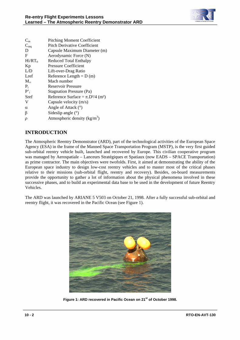
The ARD was launched by ARIANE 5 V503 on October 21, 1998. After a fully successful sub-orbital and reentry flight, it was recovered in the Pacific Ocean (see Figure 1).

Figure 1: ARD recovered in Pacific Ocean on 21st of October 1998.


RTO-EN-AVT-130 10 - 3

ARD GENERAL ARCHITECTURE

ARD aeroshape is an Apollo-70 % scaled capsule of 2.8 m diameter weighing 2.8 tons at atmospheric interface point. The search for an existing shape with available aerothermodynamic data (and especially flight data) was driven by a very challenging schedule (development studies during 1995 and 1996) and a limited funding.

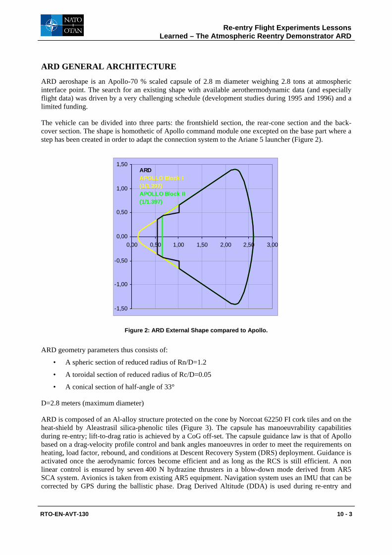
The vehicle can be divided into three parts: the frontshield section, the rear-cone section and the back-cover section. The shape is homothetic of Apollo command module one excepted on the base part where a step has been created in order to adapt the connection system to the Ariane 5 launcher (Figure 2).

-1,50

-1,00

-0,50

0,00

0,50

1,00

1,50

0,00 0,50 1,00 1,50 2,00 2,50 3,00

ARDAPOLLO Block I (1/1.397)APOLLO Block II (1/1.397)

Figure 2: ARD External Shape compared to Apollo.

ARD geometry parameters thus consists of:

• A spheric section of reduced radius of Rn/D=1.2

• A toroidal section of reduced radius of Rc/D=0.05

• A conical section of half-angle of 33°

D=2.8 meters (maximum diameter)

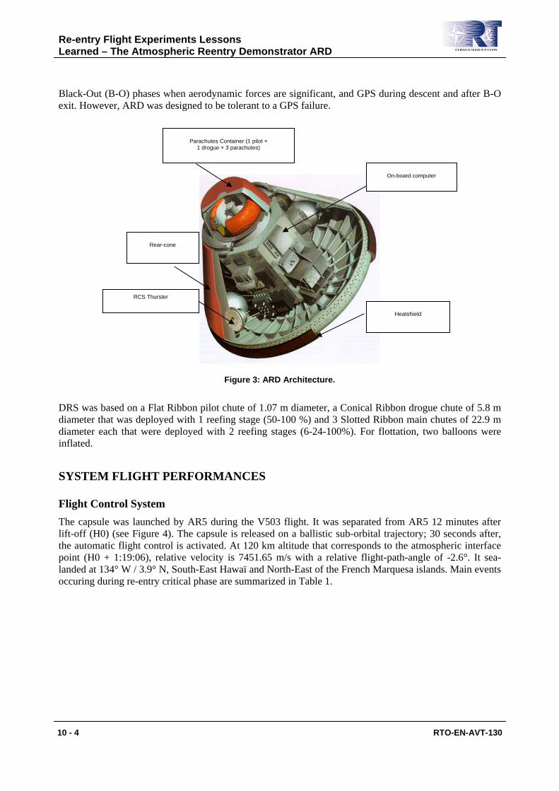
ARD is composed of an Al-alloy structure protected on the cone by Norcoat 62250 FI cork tiles and on the heat-shield by Aleastrasil silica-phenolic tiles (Figure 3). The capsule has manoeuvrability capabilities during re-entry; lift-to-drag ratio is achieved by a CoG off-set. The capsule guidance law is that of Apollo based on a drag-velocity profile control and bank angles manoeuvres in order to meet the requirements on heating, load factor, rebound, and conditions at Descent Recovery System (DRS) deployment. Guidance is activated once the aerodynamic forces become efficient and as long as the RCS is still efficient. A non linear control is ensured by seven 400 N hydrazine thrusters in a blow-down mode derived from AR5 SCA system. Avionics is taken from existing AR5 equipment. Navigation system uses an IMU that can be corrected by GPS during the ballistic phase. Drag Derived Altitude (DDA) is used during re-entry and


10 - 4 RTO-EN-AVT-130

Black-Out (B-O) phases when aerodynamic forces are significant, and GPS during descent and after B-O exit. However, ARD was designed to be tolerant to a GPS failure.

Figure 3: ARD Architecture.

DRS was based on a Flat Ribbon pilot chute of 1.07 m diameter, a Conical Ribbon drogue chute of 5.8 m diameter that was deployed with 1 reefing stage (50-100 %) and 3 Slotted Ribbon main chutes of 22.9 m diameter each that were deployed with 2 reefing stages (6-24-100%). For flottation, two balloons were inflated.

SYSTEM FLIGHT PERFORMANCES

Flight Control System The capsule was launched by AR5 during the V503 flight. It was separated from AR5 12 minutes after lift-off (H0) (see Figure 4). The capsule is released on a ballistic sub-orbital trajectory; 30 seconds after, the automatic flight control is activated. At 120 km altitude that corresponds to the atmospheric interface point (H0 + 1:19:06), relative velocity is 7451.65 m/s with a relative flight-path-angle of -2.6°. It sea-landed at 134° W / 3.9° N, South-East Hawaï and North-East of the French Marquesa islands. Main events occuring during re-entry critical phase are summarized in Table 1.

Parachutes Container (1 pilot + 1 drogue + 3 parachutes)

On-board computer

RCS Thurster

Heatshield

Rear-cone


RTO-EN-AVT-130 10 - 5

Figure 4: ARD Mission Profile.

Table 1: Main events during re-entry

EVENT TIME(s)

Z (km) MACH

Z=120km point 4750 120.0 19.5

Beginning of black-out 4845 89.8 27.4

Beginning of reentry piloting 4886 78.2 26.1

Manoeuvre #1 5062 51.6 15.0

Manoeuvre #2 5076 49.6 13.5

Manoeuvre #3 5091 47.7 12.0

End of black-out 5143 40.0 7.1

Manoeuvre #5 5154 38.0 6.0

DRS deployment 5281 14.1 0.6

Splashdown 6074 0 0.02

ARD flight was nearly nominal. Figure 5 presents the ARD trajectory ground track comparison between prediction and flight. It can be observed that at injection, the capsule was slightly foreward prediction that forced the flight control to place the capsule on a more diving trajectory.


10 - 6 RTO-EN-AVT-130

During the flight, GPS was available except during Black-Out and thus was used for altitude determination. However, post-flight analysis work has also shown that DDA and pressure sensors-based navigation have worked properly and would have been a performant back-up solution to GPS in case of non availability of it as illustrated in Figure 6.

Figure 5: ARD trajectory ground track.

IMU Altitude updated thanks to DDA

Figure 6: IMU up-date using DDA (w/o GPS).


RTO-EN-AVT-130 10 - 7

As far as propulsion system is concerned, Figure 7 shows that prediction and flight consumptions were consistent. Higher consumption than expected however occurred during the orbital phase after ARD jettisoning, during the re-entry due to RCS higher activation in order to reduce the range (diving trajectory) and during the descent phase for wind perturbations counteracting.

Re-entry

Orbital

Figure 7: Predicted and Flight Hydrazine Consumption.

Finally, the capsule sea-landed by less than 3 km off the predicted landing point.

More details could be found in [R1].

Thermal Protection System A Thermal Protection System covers the entire vehicle. Front-shield section TPS material is made of high-density (ρ = 1600 kg/m3) ALEASTRASIL tiles which is a degradable material consisting of silica substrate impregnated of a phenolic resin. Rear-cone and back-cover sections are covered by low-density (ρ = 480 kg/m3) NORCOAT-LIEGE tiles consisting of cork impregnated of a phenolic resin. Figure 8 presents the front-shield before the flight in the integration hall in EADS-ST Aquitaine plant and after recovery where the phase change can be seen on the surface (white traces). On the rear-cone (Figure 9), one can notice the black colour due to Norcoat-Liège pyrolysis phenomenon. The capsule recovery made possible the Aleastrasil tile expertise providing significant indication on the charred layer thickness that enabled to check the global validity of the thermo-optical model developped for that material (Figure 10). This was a crucial issue as far as post-flight analysis was concerned for two reasons: the identification of the resulting margins on the TPS sizing and the reliability of the heat flux extraction from temperature measurements performed deep in the material thickness, that required an accurate thermo-optical model.


10 - 8 RTO-EN-AVT-130

Figure 8: ARD Front-Shield TPS before and after recovery.

Figure 9: ARD Rear-Cone TPS before and after recovery.

Figure 10: Recovered Aleastrasil tile cut.


RTO-EN-AVT-130 10 - 9

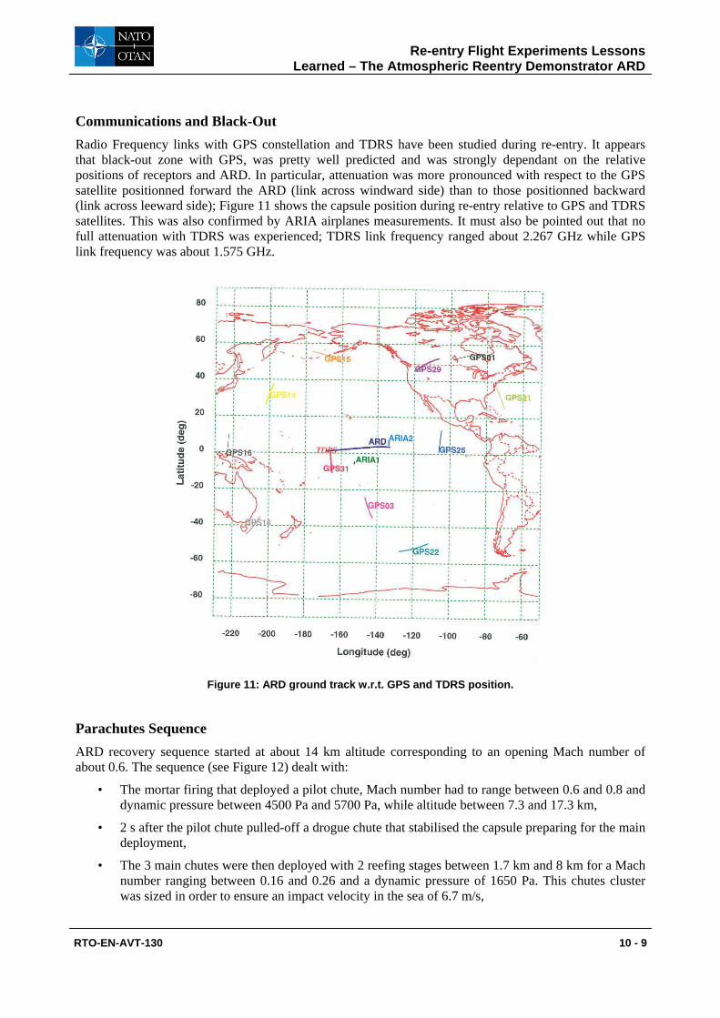
Communications and Black-Out Radio Frequency links with GPS constellation and TDRS have been studied during re-entry. It appears that black-out zone with GPS, was pretty well predicted and was strongly dependant on the relative positions of receptors and ARD. In particular, attenuation was more pronounced with respect to the GPS satellite positionned forward the ARD (link across windward side) than to those positionned backward (link across leeward side); Figure 11 shows the capsule position during re-entry relative to GPS and TDRS satellites. This was also confirmed by ARIA airplanes measurements. It must also be pointed out that no full attenuation with TDRS was experienced; TDRS link frequency ranged about 2.267 GHz while GPS link frequency was about 1.575 GHz.

Figure 11: ARD ground track w.r.t. GPS and TDRS position.

Parachutes Sequence ARD recovery sequence started at about 14 km altitude corresponding to an opening Mach number of about 0.6. The sequence (see Figure 12) dealt with:

• The mortar firing that deployed a pilot chute, Mach number had to range between 0.6 and 0.8 and dynamic pressure between 4500 Pa and 5700 Pa, while altitude between 7.3 and 17.3 km,

• 2 s after the pilot chute pulled-off a drogue chute that stabilised the capsule preparing for the main deployment,

• The 3 main chutes were then deployed with 2 reefing stages between 1.7 km and 8 km for a Mach number ranging between 0.16 and 0.26 and a dynamic pressure of 1650 Pa. This chutes cluster was sized in order to ensure an impact velocity in the sea of 6.7 m/s,


10 - 10 RTO-EN-AVT-130

• In order to mitigate g-load at sea impact, one bridle was cut just before impact so that the capsule presents a non horizontal attitude w.r.t. the sea.

DESCENT SCENARIO

Figure 12: Descent Events Sequence Definition.

DRS flight performances were assessed in terms of inflation loads and descent rates. Accelerometers, gyros, bridles strain gages, atmospheric sounding and video record have been used to retrieve flight capsule position and attitude, linear and angular velocities, relative parachute motion, amplitude and frequency of oscillations, and direction of tensile loads applied to the capsule. Figure 13 presents the flight reconstruction inflation load for the drogue chute deployment with the reefing stage with a scaling factor of 0.792 on drag coefficient that is consistent with Apollo data.

5280 5290 5300 5310 5320 5330 5340 5350 5360 53700

5

10

15

20

25

30

35

40

Time [s]

Ris

er L

oad

[kN

]

Drogue Phase - Riser Load

0.792

Figure 13: Drogue Riser Load Reconstruction (by Alénia).


RTO-EN-AVT-130 10 - 11

In order to achieve the required performances, a triggering algorithm has been developped based on:

• IMU and GPS altitude detection

• IMU and DDA (Drag Derived Altitude) according to following scheme:

• IMU and 3 Pressure measurements on the front-shield according to following scheme

The basic principle to determine the decision criteria was to impose in any case a probability of opening above M=0.8 lower than 0.5 % (see [R2]).

The descent sequence was finally triggered by a GPS up-dated navigation at an estimated altitude of 14.1 km (Z > 6 km required) and a Mach number of 0.65 (M < 0.8 required).

AERODYNAMIC RESTITUTION Aerothermodynamic flight objectives were oriented toward the improvement and validation of our aerothermodynamic tools and methodology. All the topics have been reviewed during the Post-Flight Analysis (PFA) activity, except the Dynamic Stability one, due to short funding and the lack of the whole pertinent information (no sufficient accuracy on wind profile for instance) to study the problem. It is recalled that this is an important concern for capsule-type vehicle behaviour, due to the potential dynamic instability (Cmq>0) in the low supersonic – subsonic range. It must be pointed out that this post-flight analysis work has also taken benefit from the ESA preparation programme MSTP dedicated to aerodynamic tools (both experimental and numerical issues) for Earth entry capsules led by EADS-ST from 1996 to 1998 (see [R3]).

Pre-Flight Aerodynamic Database Pre-Flight ARD Aerodynamic DataBase (AEDB) was derived from Apollo. It was built-up as follows:

• Mach 29 : the results at this point come from the analysis of APOLLO capsule flight results; then, they are supposed to contain all the physical phenomena involved during actual flight, and especially the real gas effects,

• Mach 10 : following a general trend, at this low Mach number, the flow was supposed to obey the perfect gas behaviour ; no specific study was performed about potential real gas effects,

• Between Mach 10 and 29: an interpolation process was specified.

The reference quantities used to reduce the aerodynamic forces and moments into coeffients are:

• reference length = maximum diameter (D) – Lref = D = 2.8 m

• reference surface = π.D²/4 – Sref = 6.1575 m²

P static

P atmos

Altitude

Pressure Flowfield Kp

Atmosphere P(Z)

Mach Traj

P static

P atmos

Altitude

Pressure Flowfield Kp

Atmosphere P(Z)

Mach Traj

Acc. γx

ρ atmos

Altitude

Aerodynamics CA

Atmosphere r(Z)

Altitude

Timer

Mach Traj

Acc. γx

ρ atmos

Altitude

Aerodynamics CA

Atmosphere r(Z)

Altitude

Timer

Mach Traj


10 - 12 RTO-EN-AVT-130

ARD Re-entry Trajectory The ARD trajectory parameters have been retrieved through on-board inertial navigation system measurements (IMU) and a GPS receiver operated out of the black-out period. The inertial system insured very accurate position, velocity and attitude reconstruction derived from acceleration measurements, in association with the GPS data.

The ARD reentry trajectory is presented on Figure 14 and Figure 15 in terms of time, altitude, velocity, Mach number and attitude. The aerodynamic reentry begins at 120km of altitude. Actually the pressure data were not exploitable above 90km due to the level of sensitivity of the pressure transducers.

T:[s]

V:[m

s-1]

4900 4950 5000 5050 5100 5150 5200 52500

1000

2000

3000

4000

5000

6000

7000

8000

1520253035404550556065707580 Z (Km)

61012152024 5 2 126 Mach

Figure 14: ARD reentry trajectory.

12 3

5

T:[s]

AoA

:[°]

4900 4950 5000 5050 5100 5150 5200 5250-25

-24

-23

-22

-21

-20

-19

-18

-17

-16

-15

InstantaneousMean

1520253035404550556065707580 Z (Km)

61012152024 5 2 126 Mach

Figure 15: ARD angle-of-attack time history.


RTO-EN-AVT-130 10 - 13

The Figure 15 displays the mean angle-of-attack in red and the instantaneous angle of attack in grey. The oscillations of the angle-of-attack signal are not caused by electrical noise but are representative of the actual flight attitude behaviour characterised by 0.6 Hz frequency oscillations; to avoid high hydrazine consumption RCS was activated only when the gap between the assessed attitude and the control was greater than a threshold value.

Figure 15 indicates also the maneuvers that were performed at Mach numbers 15 – 13.5 – 12 – 6 (the fourth maneuver planned at Mach number 8 was cancelled due to a control priority conflict). These maneuvers were intented to improve aerodynamic characteristics restitution; they were initiated by a RCS pulse in pitch, followed by the switch-off of FCS in order to get a pure aerodynamic behaviour.

Dynamic Pressure Reconstruction The dynamic pressure Pdyn = ½.ρ.V² is a prime parameter to retrieve the aerodynamic coefficients from the acceleration measurements.

The dynamic pressure is then the combination of the velocity and the free stream density. If the velocity is accurately derived from the on-board acceleration measurement (IMU), the density is not trivial to be obtained as no direct measurements are available for this quantity.

Four different methods have been used to assess the atmospheric density [R4]:

• Atmospheric soundings by balloon

• Atmospheric models CIRA88 and US76 Std Atm

• Model based on an “Inertial approach”

• Model based on a “Stagnation pressure approach”

The PFA pressure activity has pointed out the lack of confidence in the atmospheric models density description, and the need for more precise density assessment.

Two specific approaches were found to be consistent:

• the “inertial” approach, where the density is deduced from the acceleration measurements of the drag force, and the assumption of knowledge of the drag coefficient, given by the preflight AErodynamic Data Base (AEDB), through the relation : Drag = ½.ρ.V².Sref.CD

• the “stagnation pressure “ approach where the density is deduced from the stagnation pressure PST measurement, and the assumption of stagnation pressure coefficient Kp given by the chemical equilibrium flowfield, through the relation : KpEq = (PST – P∞) / ½.ρ.V²

The velocity V involved in both approaches is given by IMU data.

Figure 16 shows a comparison of the dynamic pressures obtained with the density computed by the various methods. A rather large dispersion (∼10%) is observed between the atmospheric models. Coherency between the “inertial” density and the “Equilibrium” density is obtained. The discrepancy between the two is less than 3.4% in the hypersonic range. The inertial and equilibrium profiles are coherent with each others all along the reentry. Unlike the atmospheric models they account for the wind perturbations (around 25km) as they are linked to the load factor (inertial) or the stagnation pressure (equilibrium) which are sensitive to wind gusts.


10 - 14 RTO-EN-AVT-130

1520253035404550556065707580 Z (Km)

61012152024 5 2 126 Mach

T:[s]

Pdy

n:[P

a]

4900 4950 5000 5050 5100 5150 5200 52500

1000

2000

3000

4000

5000

6000

7000

8000

9000

10000

11000

12000

CIRA88US76"Inertial""EQuilibrium"

Figure 16: Dynamic pressure.

When we look at the stagnation pressure, the discrepancies are more obvious. The Figure 17 displays the stagnation pressure coefficient computed with the two atmospheric models, the inertial approach and the theoretical equilibrium and perfect gas methods.

1520253035404550556065707580 Z (Km)

61012152024 5 2 126 Mach

T:[s]

Kp S

P

4900 4950 5000 5050 5100 5150 5200 52501.5

1.6

1.7

1.8

1.9

2

2.1

CIRA88US76"Inertial""EQuilibrium""Perfect Gas"

Figure 17: Stagnation pressure coefficient.

The atmospheric models lead to very scattered Kp profile with non-physical levels. The US76 model overestimates the theoretical levels while the CIRA88 model underestimates the perfect gas level around Mach 20. Consequently the atmospheric models were not appropriate for accurate pressure coefficient analysis required for perfect gas/real gas discrimination.

The inertial approach is consistent with the equilibrium level in the hypersonic range. It lies within the two theoretical models. In addition it provides with rigorous uncertainties identification and quantification (AEDB uncertainties).


RTO-EN-AVT-130 10 - 15

Figure 18 shows the inertial dynamic pressure profile and its associated uncertainty used for the pressure coefficient analysis. The inertial approach leads to a physical nominal value of the stagnation pressure coefficient.

1520253035404550556065707580 Z (Km)

61012152024 5 2 126 Mach

T:[s]

Pdy

n:[P

a]

4900 4950 5000 5050 5100 5150 5200 52500

2500

5000

7500

10000

12500

T:[s]

Pdy

n:[P

a]

4900 4950 5000 5050 5100 5150 5200 52500

2500

5000

7500

10000

12500

T:[s]

Pdy

n:[P

a]

4900 4950 5000 5050 5100 5150 5200 52500

2500

5000

7500

10000

12500

"Inertial""Inertial" uncertainties

Figure 18: “Inertial” Dynamic Pressure.

For aerodynamic coefficient reconstruction, the “stagnation pressure” approach is chosen, because of no a priori assumption about the aerodynamic characteristics of the vehicle.

Pressure Field Analysis and Real Gas Effects Identification The analysis focuses on the heat-shield as the cone and back-cover flight data are very poor due to the lack of sensitivity of the pressure sensors. For each Mach/altitude condition a flight data point, which matches the CFD attitude and Mach number, has been chosen to be compared to the CFD results. An angle of attack of 20° has been selected for all comparisons.

CFD Reconstruction

Extensive comparisons have been made all along the trajectory by the use of the pressure coefficient. The Kp allows absolute levels comparisons between numerical results obtained at the same trajectory point. Priority has been given to the symmetry plane as it maximises the discrepancies between CFD hypothesis.

The flight Kp involved in the comparisons below are obtained by the inertial approach. The associated flight error bars are induced by the uncertainties of the pre-flight aerodynamic database (Drag coefficient), the quantum of the measurement and the dispersion of the atmospheric pressure. As the quantum contribution is rather limited compared to the dynamic pressure restitution, the uncertainties on the Kp act as a constant percentile bias for all the sensors at a given altitude. Therefore the profiles structure of the flight data points are meaningful even if the absolute Kp level is doubtful.

Figure 19 shows CFD comparisons at Mach 10. The real gas effect is clearly displayed on the stagnation region. Small discrepancies are observed on the real gas profiles between the results of computations performed by EADS-ST and by ESA/ESTEC. No discrepancies are found between the NEQ cases of ESTEC which suggests that the Euler/Navier-Stokes models have a small impact on the heat-shield


10 - 16 RTO-EN-AVT-130

pressure field at Mach 10. Thin boundary layer is expected in this region of the capsule at hypersonic regime.

PG

RG EQ

LEEWARD S/D WINDWARD

Pre

ssur

eC

oeffi

cien

t

-1.25 -1 -0.75 -0.5 -0.25 0 0.25 0.5 0.75 1 1.25-0.20

0.00

0.20

0.40

0.60

0.80

1.00

1.20

1.40

1.60

1.80

2.00

2.20EUL PGA M10 FL ESTEL1EUL RGE M10 FL AML1EUL NEQ M10 FL ESTEL2NSL NEQ M10 1500 ESTEL31

T=5106.56,M=10.39,α=20.36,β= .26

Figure 19: Kp Mach 10.

Figure 20 and Figure 21 display CFD results at Mach 15. The real gas effect magnitude is increased at this Mach/altitude condition compared to Mach 10. Very good coherency is observed between the real gas results with limited dispersion. Discrepancies between the various real gas cases are mainly caused by pressure field oscillations and it is difficult to estimate the impact of the Euler/Navier-Stokes modelisations on the heat-shield pressure field.

PG

RG EQ


Pre

ssur

eC

oeffi

cien

t

-1.25 -1 -0.75 -0.5 -0.25 0 0.25 0.5 0.75 1 1.25-0.20

0.00

0.20

0.40

0.60

0.80

1.00

1.20

1.40

1.60

1.80

2.00

2.20EUL PGA M15 FL EPFL12EUL RGE M15 FL AML2EUL NEQ M15 FL20 ESTEL5

T=5062.13,M=15.01,α=19.99,β= -.08



RTO-EN-AVT-130 10 - 17

PG

RG EQ


Pre

ssur

eC

oeffi

cien

t

-1.25 -1 -0.75 -0.5 -0.25 0 0.25 0.5 0.75 1 1.25-0.20

0.00

0.20

0.40

0.60

0.80

1.00

1.20

1.40

1.60

1.80

2.00

2.20NSL NEQ M15 FL 1500 ESTEL32NST RGE M15 FL DLR6NST NEQ M15 FL DLR20

T=5062.13,M=15.01,α=19.99,β= -.08

Figure 21: Kp Mach15 (concluded).

The real gas effects are maximised in the symmetry plane by the Mach 24 cases as displayed by Figure 22 and Figure 23. For this Mach/altitude condition, numerical convergence is more problematic and pressure field oscillations near the stagnation point and on the leeward side of the heat-shield are often found in the CFD results. However a good overall coherency between the contributors is observed. It is tough to discriminate between the real gas modelisations impact on the heat-shield pressure field and the code/mesh effects.

PG

RG EQ


Pre

ssur

eC

oeffi

cien

t

-1.25 -1 -0.75 -0.5 -0.25 0 0.25 0.5 0.75 1 1.25-0.20

0.00

0.20

0.40

0.60

0.80

1.00

1.20

1.40

1.60

1.80

2.00

2.20EUL PGA M24 FL20 ESTEL19EUL RGE M24 FL AML3EUL NEQ M24 FL AML4

T=4942.43,M=24.05,α=20.09,β= .69



10 - 18 RTO-EN-AVT-130

PG

RG EQ


Pre

ssur

eC

oeffi

cien

t

-1.25 -1 -0.75 -0.5 -0.25 0 0.25 0.5 0.75 1 1.25-0.20

0.00

0.20

0.40

0.60

0.80

1.00

1.20

1.40

1.60

1.80

2.00

2.20NSL RGE M24 FL DLR15NSL NEQ M24 FL20 ESTEL13NSL NEQ M24 FL DLR10

T=4942.43,M=24.05,α=20.09,β= .69

Figure 23: Kp Mach 24 (concluded).

Regarding the real gas effects, the larger impact is expected to be found at high Mach/high altitude (low density) as suggested by Figure 17. The discrepancies between the real gas and the perfect gas hypothesis increase with the altitude along the ARD re-entry trajectory. On Figure 22 the impact of the chemical hypothesis at Mach 24 is clearly displayed. The stagnation Kp is increased by 5.5% while the stagnation point is shifted in the direction of the windward side.

Figure 24 shows Kp profiles comparisons at various Mach numbers for real gas ESTEC (Lore) CFD Navier-Stokes results implemented with a chemical non-equilibrium model. This graph provides a clear view of the evolution of the flow field absolute pressure level as a function of the Mach number without code/mesh effects. The main impact on the pressure coefficient is localised in the stagnation point region. The stagnation point shifts in the direction of the windward side and the stagnation pressure increases with the Mach number. The evolution of the stagnation pressure with the Mach number complies with the expected theoretical rate. In addition low Mach number sensitivity is found in the centre of the heat-shied while the Kp level of the leeward shoulder (tore) tends to decrease with the Mach number. The pressure coefficient profile in the symmetry plane is then modified in a non-uniform way. The modification of the Kp profiles has a direct impact on the relative pressure distribution.


RTO-EN-AVT-130 10 - 19


Pre

ssur

eC

oeffi

cien

t

-0.5 -0.25 0 0.25 0.5

0.80

1.00

1.20

1.40

1.60

1.80

2.00NSL NEQ M10 1500 ESTEL31NSL NEQ M15 FL 1500 ESTEL32NSL NEQ M20 FL 1500 ESTEL29NSL NEQ M24 FL20 ESTEL13

Figure 24: Kp Mach effect on pressure distribution.

A significant effect is observed on the leeward distribution between Mach 10 and Mach 15. The leeward relative pressure decreases when the Mach number increases. In addition the expansion on the windward tore is stronger when the Mach increases. This behaviour is weaker above Mach 15 but a clear monotonous effect is found. Thereafter the real gas effects alter the relative pressure distribution of the heat-shield expansion zones of real gas computations. This behaviour is not found for perfect gas results and is not the consequence of viscous/boundary layer effects.

Consequently real gas “markers” have been defined through CFD analysis. A summary of these CFD real gas “markers” is given in the following table with the associated flight pressure sensors (see Figure 25).

MARKER PARAMETER

MARKER LOCATION

EFFECT (MACH INCREASE)

FLIGHT SENSOR(S)

SP Increase P1, P3

Tore Increase P4 Kp

Tore Decrease P16, P17

Tore Increase P4

P/Pi

Heat-shield Decrease P16, P17


10 - 20 RTO-EN-AVT-130

Figure 25: Pressure Taps Location.

High Enthalpy Testing

Wind tunnel tests have been performed at ONERA F4 and DLR HEG high enthalpy facilities. The objectives of the testing were to measure skin pressure and heat-fluxes at high enthalpy in order to experience real-gas effects in ground facilities.

Two reference conditions have been tested for each wind tunnel. They are summarised in the following table.

WT CONDITION F4 II

F4 III

HEG III

HEG I

Pi (bar) 600 400 490 400

Hi/RT0 60 150 170 280

M∞ 12.1 8.6 8.2 8.2

ρ∞ (kgm-3) 2.7 10-3 6.1 10-4 3.3 10-3 1.7 10-3

V∞ (ms-1) 3 000 4 700 4 800 6 000

P’i (kPa) 33.9 25.5 79.3 60.0

The complementary F4 and HEG conditions cover a wide reduced enthalpy range from 60 to 280. The associated levels of dissociation are favourable to the occurrence of real gas effects.

Figure 26 (F4) and Figure 27 (HEG) display the dispersion of the P/Pt parameter where Pt is the wind tunnel reference stagnation pressure (pitot pressure).


RTO-EN-AVT-130 10 - 21


P/P

t

-1 -0.75 -0.5 -0.25 0 0.25 0.5 0.75 1-0.1

0

0.1

0.2

0.3

0.4

0.5

0.6

0.7

0.8

0.9

1

1.1

1.2R1041, T= 60ms, HiR= 78, Pi=649barR1041, T= 90ms, HiR= 56, Pi=540barR1046, T= 40ms, HiR=149, Pi=409barR1046, T= 60ms, HiR=137, Pi=344bar

F4

Figure 26: ONERA F4 relative pressure profile.


P/P

t

-1 -0.75 -0.5 -0.25 0 0.25 0.5 0.75 1-0.1

0

0.1

0.2

0.3

0.4

0.5

0.6

0.7

0.8

0.9

1

1.1

1.2R582, HIR=167, Pi=492bar, Cond IIIR583, HIR=280, Pi=382bar, Cond I HEG

Figure 27: DLR HEG relative pressure profile.

It is inferred from these comparisons that the pressure coefficients do not provide enough confidence to clearly discriminate between perfect gas and real gas pressure field distribution. However the pressure levels on the tore section in the symmetry plane are consistent with real gas distributions.

Real Gas Effects

The real gas effects depend on the dissociation of the air chemical components in the shock layer. They have a direct impact on the level and position of the stagnation pressure as the distance between the body and the shock is modified by the chemical activity in the shock layer.

The same approach as for the CFD results has been used for the flight data set in order to identify real gas effects. The real gas markers identified for the real gas CFD cases have been looked for through extensive


10 - 22 RTO-EN-AVT-130

comparisons between several trajectory points. As the flight pressure coefficients are not accurate enough for flight/flight comparisons, the relative pressure parameter has been chosen.

CFD studies have shown that the real gas effects are imbedded within the relative pressure profile, particularly in the symmetry plane in the expansion zones of the tore section. The main problem for meaningful comparison is the sensitivity of the pressure field structure to the attitude of the capsule. Therefore systematic relative pressure profiles comparisons have been performed between data points with the same angle of attack and the same side slip angle absolute value. It is observed that the real gas CFD markers are found on every iso-attitude comparisons.

In order to ease the identification of the real gas effects a new parameter based on differential pressure measurements has been created. It is defined by:

Pi

17P4PparameterGasReal −=

This parameter combines the two antagonist real gas markers and thus maximises the observation of the real gas effects. The main disadvantage of this parameter is that it is highly sensitive to the attitude.

Figure 28 shows the evolution of the real gas parameter as a function of the reduced enthalpy Hi/RT0 (RT0 = 78 328.2 j/kg). The reduced enthalpy is representative of the amount of energy imbedded in the upstream flow-field and thus allows comparisons between flight/CFD data and the wind tunnel data. It has to be noticed that the uncertainties related to the absolute WT restitution are rather large. Moreover the upstream conditions of the two facilities run conditions are not the same and have an impact on the pressure distribution on the heat-shield. Thereafter the absolute levels should not be considered but the relative levels from one run condition to another for each facility. The CFD cases show the trends identified during the CFD analysis. As expected the perfect gas computations do not alter the perfect gas parameter whereas the real gas cases show an increase of the parameter when the Mach number varies. Same behaviour is observed for both real gas chemical hypothesis. The flight data points plotted on the graph are the only points available at this specific attitude. Same trend is observed for the wind tunnel results than for the CFD data and the flight measurements from Mach 10 to Mach 24. When the energy increases, the real-gas parameter increases. This behaviour is clearly identified in the experimental ground data when the enthalpy condition varies. Real gas effects are then identified between Mach 10 and Mach 24 on both CFD and flight data. The ground facilities results are coherent with the flight measurements.

F4 IIIF4 III

F4 IF4 I

HEG III

HEG II

Perfect Gas

Real Gas NEQ

Real Gas EQ

Hi/RT0

∆P/P

'i 4/17

40 60 80 100 120 140 160 180 200 220 240 260 280 300 320 3400.26

0.27

0.28

0.29

0.3

0.31

0.32

0.33

0.34

0.35

0.36

0.37

0.38ESTEC LORE EUL PGELV RG EUL EQESTEC LORE EUL NEQESTEC LORE NSL NEQFLIGHT α=19.8, β=0.2FLIGHT α=20.0, β=0.6

Figure 28: Real gas parameter.

17

4


RTO-EN-AVT-130 10 - 23

The problem of the Mach number threshold to observe real gas effects in the flight data set is rather difficult to address. The range of the available attitudes changes below Mach 10 as the mean angle of attack increases. Thereafter the real gas parameter does not allow any comparison between CFD and flight data because no AoA/SSA complies with the attitude of the CFD database. However systematic flight to flight iso-attitude comparisons show that the real gas markers can hardly be distinguished below Mach 8. Consequently the real gas effects are discernible above Mach 8 on the flight data. This Mach number threshold is conservative in a sense that chemical effects may occur below Mach 8.

AERODYNAMIC FORCE COEFFICIENTS RESTITUTION [R5]

The aerodynamic force coefficients are assessed through the acceleration measurements of IMU giving forces in the frame trihedron, and using the dynamic pressure based on the “stagnation pressure” atmospheric density:

FA,N = ½.ρ.V².Sref.CA,N

The uncertainties on the aerodynamic force coefficients are related mainly to the restitution of the dynamic pressure. Indeed, aerodynamic force restitution is based on accurate acceleration and attitude measurements, combined with well defined mass model taking into account the FCS ergol consumption.

The preflight AEDB was based on Mach 10 perfect gas result in the whole hypersonic range. No real gas effect was taken into account on nominal coefficients CA and CN. Only the uncertainty level was increased at Mach 29 to account for these potential effects.

A general overview of the results shows that the reconstructed axial and normal force coefficients lie within the preflight AEDB uncertainty band. The trend of both coefficients is coherent with the predicted ones. Actually, the dynamics of the coefficients is mainly governed by the AoA evolution along the trajectory. However, regarding the axial coefficient, a higher absolute slope is observed for the flight reconstructed value, suggesting a real gas effect in flight, not taken into account in the preflight AEDB.

All CFD results comply with the preflight AEDB uncertainty band. For the normal force coefficient, the flight/AEDB/CFD discrepancy is low compared to the AEDB uncertainty level. Larger discrepancies are noticed for the axial force coefficient.

The CFD increase of axial force coefficient with the Mach number is coherent with the reconstructed flight data, indicating that the CFD real gas effects are coherent with the flight ones.

No definitive advantage is found for viscous assumption. The level of flight uncertainties does not allow to discriminate between Euler and Navier-Stokes modelisations.

For axial force coefficient, it can be seen that the CFD perfect gas level does not match the reconstructed values, which are more comparable to the real gas assumptions one. This is an indication of some real gas effects on this coefficient for Mach number greater than 6. As another consequence, it could be possible to reduce the lower uncertainty band of preflight AEDB, by considering the lowest level as given by the perfect gas level.

For the normal force coefficient, the discrepancy between flight, CFD and preflight AEDB data seems low, and much lower than the AEDB uncertainty level. But the results are not fully coherent with the axial coefficient ones; CFD-flight CN matching seems to be the best when a Non-equilibrium assumption is considered, while the CA matching is the best for an Equilibrium assumption. Moreover, for CN, the discrepancy between Equilibrium and Non-equilibrium is much higher than for CA. It has to be recalled that the CN is much more sensitive to the pressure flowfield on the rear conical part of the capsule than the


10 - 24 RTO-EN-AVT-130

CA; this part of the vehicle is quite difficult to compute, and the comparison with the flight results in terms of pressure field is not so good, so that the CN CFD result cannot be considered as fully realistic.

Mach number

CA

4681012141618202224261.28

1.30

1.32

1.34

1.36

1.38

1.40

1.42

1.44ReconstructionAEDB FLT AoAAEDB 20° AoAEUL PGEUL EQEUL NEQEUL NEQ 19°NS PGNS EQNS EQ 19°NS NEQ

Figure 29: Axial Force Coefficient Evolution with Mach number.

Mach number

CN

468101214161820222426-0.13

-0.12

-0.11

-0.10

-0.09

-0.08

-0.07

-0.06

-0.05

-0.04

ReconstructionAEDB FLT AoAAEDB 20° AoAEUL PGEUL EQEUL NEQEUL NEQ 19°NS PGNS EQNS EQ 19°NS NEQ

Figure 30: Normal Force Coefficient Evolution with Mach number.

HYPERSONIC TRIM [R5] The maneuver capability of the capsule is driven by the lift-over-drag ratio which may be drastically affected by the real gas effects through the following way:

Real Gas Effects ==> Cm(α) ==> αtrim ==> L/Dtrim


RTO-EN-AVT-130 10 - 25

The flight analysis has been oriented with the following objectives:

• Identification of real gas effects on hypersonic trim,

• Validation of preflight predictions,

• Assessment of CFD results.

The flight AoA results are given on Figure 31, showing the flight oscillation history, from which a mean AoA has been deduced.

ARD - Angle-of-AttackComparison Flight - Prediction

-30,0

-28,0

-26,0

-24,0

-22,0

-20,0

-18,0

-16,0

-14,0

-12,0

-10,0

4850,0 4900,0 4950,0 5000,0 5050,0 5100,0 5150,0 5200,0 5250,0 5300,0

Time (s)

Ang

le-o

f-Atta

ck (°

)

Flight AoAMean AoAMin/Max AoAPredictionPrediction - With DCmPrediction - With DZCoG

PredictionCoG : Take-Off

Figure 31: AoA Time History.

The mean trim AoA is compared to the postflight prediction performed using the preflight AEDB, the actual flight history V(Z) and the flight Center-og-Gravity (CoG) location at take-off. The comparison shows that the discrepancy between flight and prediction is about 1.5° to 2.0° between Mach 26 (t=4900s) and Mach 12 (t=5090s), with a predicted AoA higher (in absolute value) than the flight result. This discrepancy is decreasing to become null at Mach 5. In supersonic regime, the predicted AoA becomes lower (in absolute value) than the flight one (less than 1°).

Two Contributors may be considered to explain the discrepancy:

• The aerodynamic characteristics, and mainly the pitching moment coefficient ; a value of ∆Cm< 0.006 (which is the preflight AEDB uncertainty at high Mach number) would be appropriate,

• The CoG location ; a value of ∆ZCoG< 10mm (which is the preflight uncertainty) would be appropriate.

The effect of these contributors is shown on Figure 31, with the following values resulting from preflight assessment:

∆Cm = 0.003 4 < Mach < 10

∆Cm = 0.006 10 < Mach

∆ZCoG = 10 mm


10 - 26 RTO-EN-AVT-130

The flight prediction discrepancy could be explained by parameter variations well within the preflight uncertainty domain. This is an important result that shows that the uncertainty sizing was well performed and that the safety of flight was fully insured.

It is suggested that the flight prediction discrepancy could be due to a combination of CoG location bias and of Cm misprediction.

Flight CoG Assessment

The CoG location is a driving parameter for the assessment of trim AoA. During the flight, the mass and centering of the capsule is subject to changes due to two specific phenomena: the consumption of the ergols used for the capsule control, and the pyrolysis of the heatshield under aerothermal heating. A model for ergol consumption was given by the flight control analysis.

For heatshield pyrolysis, a model has been built using results of the heatshield postflight expertise that gave the depth of the pyrolysed zone at two specific thermocoils location, so that an assessment of total mass loss could be performed.

The following analysis has been performed with a flight “nominal” CoG location (referred as CoG#2) derived from the combination of these two models.

CFD Reconstruction

Figure 32 gives a comparison, in term of trim AoA, between flight and numerical simulation results. This Figure includes:

• The flight AoA along the trajectory,

• The prediction obtained with the preflight AEDB,

• The prediction given by the Mach numbers 10 and 29 data of the preflight AEDB,

• The results of the numerical simulations defined in the PFA computation plan,

• The results of the MSTP study (see [R3]).

ARD - Angle-of-AttackComparison Flight - Prediction - Numerical Simulation

-30,0

-28,0

-26,0

-24,0

-22,0

-20,0

-18,0

-16,0

-14,0

-12,0

-10,0

4850,0 4900,0 4950,0 5000,0 5050,0 5100,0 5150,0 5200,0 5250,0 5300,0

Time (s)

Ang

le-o

f-Atta

ck (°

)

Flight AoA Mean AoA Min/Max AoAPrediction NS - RG-NEq EU - RG-NEqNS - RG-Eq EU - RG-Eq NS - PGEU - PG AEDB - Mach29 AEDB - Mach10

MSTPMSTP

CoG #2

Figure 32: Restored AoA Time History versus CFD prediction.


RTO-EN-AVT-130 10 - 27

All the computed results have been obtained with the same evolution of CoG location (CoG#2) along the trajectory, taking into account ergol consumption and heatshield pyrolysis.

The analysis of the plots leads to the following comments:

• The PFA computations under the perfect gas assumption give results quite similar to the Mach 10 AEDB data, with a quite perfect comparison at Mach 10; the slight effect observed at other trajectory points is coherent with the Mach number effect on trim AoA.

• The real gas effect, as given by the computations (MSTP and PFA) is greater than the effect contained in the preflight AEDB for Mach numbers greater than 15: this numerical real gas effect decreases when the Mach number is decreasing, and at Mach number 15 the numerical results give the same magnitude than the Mach 29 AEDB; at Mach number 10, real gas numerical results are scattered, but there is still some evidence of this effect, which was not assumed up to now.

• Except at Mach number 10, the computations performed with the assumption of real gas in chemical non-equilibrium lead to the most important effect of real gas on trim AoA, and are the closest to the flight results.

• There is no evidence of very definite viscous effect on the trim AoA, whatever the chemical assumption and the Mach number range.

The PFA computations, with the assumption of real gas effects, give an evolution of trim AoA along the trajectory that is quite similar to the flight one. These real gas effects have to be considered down to low hypersonic Mach numbers (Mach < 10).

As far as AEDB predictions are concerned, the computations show evidence of an underestimation of real gas effects at high Mach numbers and a misprediction of the evolution of these effects along the trajectory.

Likely Global Scenario

It has been seen that the computations were able to reproduce the evolution shape of the trim AoA flight results, but with an absolute value a little bit higher. This information is used as an indication of a bias in CoG location and defines the ∆ZCoG shift able to match computations and flight. A value of ∆α=0.6° seems to be necessary, leading to ∆ZCoG = +3mm, within the 10mm preflight uncertainty CoG location.

At this point there is still some discrepancy between the flight and the prediction with the preflight AEDB. This discrepancy is supposed to be due to a misprediction in aerodynamic pitching moment coefficient. Figure 33 gives the necessary ∆Cm to match AEDB prediction and flight result, taking into account the ∆ZCoG = 3mm previously defined. It is compared to similar values given by the numerical simulation with real gas assumption, either equilibrium or non-equilibrium. This comparison shows that the necessary ∆Cm is covered by the computation results, indicating on one hand that the computations are able to reproduce flight results, on the other hand a misprediction in the preflight AEDB which may be explained as follows:

• Underprediction of the real gas effects at high Mach number (Mach > 24) and at low hypersonic Mach number (Mach10 where in fact perfect gas was assumed),

• Mis-prediction at intermediate hypersonic Mach numbers, due to the underprediction at the boundaries and to the interpolation process.


10 - 28 RTO-EN-AVT-130

Pitching Moment CoefficientIncrement for Flight Restitution

-0,008

-0,006

-0,004

-0,002

0

0,002

0,004

0,006

0,008

0 5 10 15 20 25 30

Mach Number

∆C

m

Data Base UncertaintyNecessary DCmEquilibrium ComputationNon-Equilibrium Computation

CoG #2 and Delta ZCoG = 3mm

Figure 33: Pitchnig moment correction in pre-flight AEDB.

As a summary, the flight prediction discrepancy may be explained by a scenario such as:

• CoG bias ∆ZCoG = +3mm, corresponding to about one third of the discrepancy between Mach numbers 29 and 10,

• ∆Cm to better account for real gas effects, corresponding to the remaining two third of the discrepancy.

These suggested values range mainly within the preflight uncertainty data.

FLIGHT AEROTHERMAL ENVIRONMENT [R6]

Aerothermal Flight Data Flight measurements dedicated to aerothermodynamics consisted of :

• 14 plugs equipped by 3 or 5 thermocouples on Aléastrasil frontshield

• 2 plugs equipped by 2 thermocouples on Norcoat-Liège back-cover

• 4 Copper calorimeters on Norcoat-Liège conical section

• 6 TPS materials samples equipped by 2 thermocouples

• Thermo-sensitive paints and IMTK on conical section

Plugs technology was taken from EADS-ST military re-entry bodies flight experiences (see Figure 34). They are equipped by 5 to 2 thermocouples with one located close to the hot surface (about 1 mm for ALEASTRASIL and 2.6 mm for NORCOAT-LIEGE plugs). Analysis of time history of measured temperatures allows the extraction of flight convective heat flux through an ad-hoc TPS material thermal model. Calorimeters technology was taken from Ariane 5 program based on copper element thermal inertia; heat flux is derived from stored heat in the element.


RTO-EN-AVT-130 10 - 29

Figure 34: Plug Thermocouples Implantation.

Figure 35 presents a global view of the set of measurements installed on the capsule.

Figure 35: ARD Flight plugs and calorimeters location.

Measurements Flight Data As far as aerothermal measurements are concerned, following results have been obtained:

• Thermocouples responses were satisfactory for T<700°C/800°C

• As T>700°C/800°C, unexpected evolutions have been recorded (see Figure 36)

• Possible laminar to turbulent transition detection at about 5050 sec. on leeward part of frontshield.

• Theoritical prediction over-predicts temperatures on main part of re-entry, which is coherent with conservative assumptions taken in TPS sizing phase (see Figure 36)


10 - 30 RTO-EN-AVT-130

• General aspect of recovered ARD is very good; low degradation of ALEASTRASIL TPS, but surface condition rather different from pre-flight ground testing using plasma arc heat simulations (SIMOUN tests)

• Back-cover part was not recovered

Figure 36: Temperature post-flight prediction/measurements comparison.

Flight recorded data are globally of good quality, excepted for the thermocouples foreseen to exceed 700°C/800°C, making the flight convective heat flux extraction on frontshield section and over a part of the re-entry, more uncertain. Moreover, over-prediction of theoritical assessment needs to be explained, some explanations have to be examined in detail. Advantage has also been taken from capsule recovery and detailed expertise of the capsule allowed to obtain information on TPS material properties in order to help in deriving more accurate flight convective heat flux.

Flight Heating Rates Extraction Flight heating rates are extracted from the knowledges of temperatures evolution versus time from thermocouples implemented in degradable (thermal plugs) or non degradable materials (copper calorimeters). It is thus necessary to develop thermal models before any heat flux derivation. For copper calorimeters, classical 3D thermal model for the complete calorimeter has been developped from which an inverse method has been derived [R7]. The Thermal Mathematical Model accounts for external and internal radiative heat transfer, conductive heat transfer in the complete calorimeter, and non-linear thermal properties of the materials (temperature dependant conductivity and capacity). For degradable materials, an 1D approach has been selected. An inverse procedure has been especially developed that was based on existing BE13 1D thermal response code applicable on pyrolysable / ablative material. This code solves the following equations:

• The internal energy balance including pyrolysis terms. The local specific heat is formulated from functions of temperature input for both virgin material and char. In partially pyrolyzed zones (ρc<ρ<ρv), the specific heat is obtained from a mixing rule

• The Internal Decomposition Equation taking into account pyrolysis equation

• Internal Mass balance Equation where the internal decomposition converts some of the solid into pyrolysis gas.


RTO-EN-AVT-130 10 - 31

• Surface Energy Balance Equation including blocking factors due to pyrolysis and ablation products

The inverse procedure is based on the theory of optimal command and Pontriaguine principle minimizing the objective-function:

[ ] dtttxThJft

t kkkr

2

0

0

)(),(),,( ∫∑ −= θβα

where:

α0 is the unblocked convective heat transfer coefficient

hr is the recovery enthalpy

β is the cold face heat loss coefficient

Preliminary assessment of elementary uncertainties has been performed, they are due to:

• Numerical bias of the inverse procedure

• TPS material thermal model uncertainties

Combination can be derived in order to assess the total uncertainty associated to extracted heat flux. However, due to thermocouples early dysfunctionning, uncertainty on peak heat flux can not be accurately determined. Moreover, only one single SIMOUN tests has been treated with a plug differing from that of flight; this is not sufficent to correctly address the thermal properties uncertainties issues in spite of very encouraging preliminary results. It is thus believed that complementary analysis are required to address this issue.

ARD Extracted Flight Heating Rates

Inverse procedure has been applied for 16 plugs located mainly on the front-shield (14 and 2 on the NORCOAT-LIEGE back-cover section). Specific inverse procedure not decribed in this paper has been applied on the 4 copper calorimeters inserted in NORCOAT-LIEGE material on the rear-cone section.

Front-Shield section

Front-shield is the most instrumented section, it is submitted to high heating rates during re-entry. Figure 37 presents the flight extracted heating rates at 3 characteristic points along the symetry plane. The time history is uncomplete due to near hot surface thermocouples failure. In spite of these dysfunctionning, maximum heating rate instant has been extracted, occurring at about 4950 s corresponding approximatively to 64.6 km altitude and Mach number of 23.5. Maximum extracted heating rate is about 1.2 MW/m2 at T4 location. Amplification factor between T0 and T4 is about 2 which is significantly higher than predicted; ARD aerothermal database provides with amplification factor on the shoulder of about 1.7 [R8]. Moreover, laminar-to-turbulent transition is detected at T17 location on the leeward part of the front-shield. It seems to occur at about 5035 s at about 57.2 km altitude which corresponds to a Mach number of 17.8 and a Reynolds number based on diameter of 4.8 105 with transitional flow extension region ranging between 5035 s and 5065 s (Mach number of about 14.7 and Reynolds number of about 7.8 105 corresponding to 51.3 km altitude).


10 - 32 RTO-EN-AVT-130

Figure 37: Flight extracted heating rates on front-shield section.

Rear-Cone section

Rear-cone section was predicted to be submitted to moderate heating rates justifying the use of calorimeters for flight heat flux assessment. These calorimeters consist of copper elements inserted in the NORCOAT-LIEGE thermal protection material. During arc-jet SIMOUN qualification test, no influence of surrounding material on heat flux restitution have been observed, consequently, flight heat flux extraction has been performed without taking into account the effect of surrounding material [R9] (outgassing, temperature jump, catalycity…). Figure 38 presents the flight heat flux time history over the complete range of re-entry at F8, F9, F28 and F29 stations. Maximum heat flux is about 37 kW/m2 but the corresponding instant is shifted to later instant compared to the front-shield section, at about 5064 s. More over, no sudden increase of heat flux which is the mark of a laminar-to-turbulent transition is observable. The main consequence of this singular behaviour is that proportionality between front-shield section and rear-cone heat flux is not respected as proposed in [R8]. This could be due to the occurrence of a kind of transitional flow resulting in an intermediate heat flux value between laminar and turbulent regimes. An other explanation could be that thermo-chemistry or local rarefaction effects due to the rapid expansion could take place in this area. Both assumptions are discussed in next sections.

Figure 38 : Flight extracted heating rates on the rear-cone section.


RTO-EN-AVT-130 10 - 33

CFD and WT tests support for flight data analysis

On the basis of the above observations, CFD and WT test plans have been defined in order to support the flight observations.

Heating Rates Time History

From the observations on extracted heat flux and aerodynamic analysis purposes, following trajectory points have been selected for CFD re-building:

Table 2: CFD flight conditions

t(s) Alt(km) Mach issues

4888.9 77.28 26.07 Surface catalysis

4942.3 65.73 24.1 Peak heating

5005.8 60.64 20

5063.1 51.63 15

5089.9 47.73 12

5110.1 44.98 10 After-body heating

5154.3 37.96 6 Turbulent flow

It must be however recalled that ARD configuration is very difficult to compute because the main section of interest lie in a large subsonic region (front-shield). Moreover, computed heat flux are difficult to assess accurately due to remaining uncertainties on transition/turbulent modelling, and lack of robustness of non equilibrium flow computations. From the CFD plan, only the “best” computations have been retained for flight data analysis.

From these computations, heating rates time histories at each flight measurement station have been derived by an adapted interpolation procedure.

Front-Shield Section

Comparisons of extracted flight heating rates with different post-flight reconstruction at T0, T4 and T17 stations. Post-flight reconstruction consist of engineering method developped for ARD sizing [R8] and CFD computations according to different flow assumptions. Comparisons with flight data allow to draw following general trends:

• t < 4875 s: Flight heat flux are significantly lower than “equilibrium flow” (EqF) prediction. By comparing with CFD computations at Mach 26 with two different wall catalysis assumptions and an engineering method based on a frozen boundary-layer and a non catalytic surface assumption, low catalytic effects in flight are evidenced. This could be attributed to the large presence of Silica in the ALEASTRASIL material substrate.

• 4875 s < t < 4950 s: Flight heating rates suddenly increase and tend toward EqF prediction. Peak heating is achieved at about 4950 s (Mach 23.5, altitude 64.6 Km) for the 3 plugs locations. For


10 - 34 RTO-EN-AVT-130

T0 and T4 stations, flight heating rates are higher than theoritical predictions; equilibrium CFD computations result in the better agreement with flight data. This trend can be correlated to the occurrence of pyrolysis; injected pyrolysis gas start to be significant at about 4875 s. Effects of these pyrolysis gas on catalycity of the surface are not known, but it can be assumed that the pyrolyis products react with the external flow by promoting recombination of oxygen and nitrogen atoms of dissociated air making the surface apparently catalytic.

• At t=5035 s: After peak heating, laminar to turbulent transition is detected on the leeward part of the front-shield at T17 station (see Figure 41). Flight turbulent heat flux is not accurately determined due to too early thermocouple dysfunctionning, however, trends are not in contradiction with ARD aerothermal database based on enginneering methods or CFD results. However, one can notice large differences in terms of computed heat flux according to the selected gas assumptions for which CFD artefacts can not be excluded [R10].

Figure 39: T0 plug station CFD/Flight extraction comparison.



RTO-EN-AVT-130 10 - 35


Real gas effects are mainly localized in the shoulder region where gradients are magnified by the shock stand-off distance when chemistry is accounted for. Figure 42 presents a representation of real gas effects

on heating rates amplification factor 4

0

T

T

qq

versus reduced total enthalpy parameter. According to the

nominal ARD aerothermal database derived from perfect gas computations, this ratio was assumed to be constant and equal to 1.7 at 20° AoA. Flight data provide with higher amplification factor of about 2 for Hi/RT0 of about 300. This trend is confirmed by CFD results at equilibrium exhibiting amplification factors varying from 2.2 to 1.7 with decreasing total enthalpy and high enthalpy ground facilites tests in HEG for which factors of 1.82 and 2.1 have been recorded. These results confirm “a posteriori” the corrective factor value of 20 % taken for ARD TPS sizing in order to account for real gas effects at equilibrium [R8]. These results also exhibit the capability of european HEG facility to capture real gas effects on capsule heat flux distribution which is very encouraging for any future projects.

Figure 42: Real gas effects on shoulder heating rates.


10 - 36 RTO-EN-AVT-130

Rear-Cone Section

Figure 43 presents the comparison of flight extracted heating rates from calorimeters with post-flight reconstruction at F8 station. Figure shows that from beginning of re-entry, flight heating rates almost follow the laminar equilibrium prediction until 4950 s after which the curves tend to diverge; computation predicts a decrease of heating rates whereas flight data indicate a continuing increase until 5050 s after which a decrease is observed. The main consequence of this relative discrepancy deals with the total heat load for which laminar prediction results in an under-estimation of this parameter. For TPS sizing, laminar to turbulent transition was assumed to occur at the same instant than that on front-shield and consequently, this relative under-estimation of heat load was covered by turbulent heat flux assumption. However, the sudden increase of heat flux due to this transition is not observed in flight, and origin of this flight behaviour is presently unexplained. Two explanations can be advanced: the first deals with the occurrence of a transitional flow resulting in an intermediate heat flux between laminar and fully turbulent regimes. This assumption seems to be corroborated by the detection of transition on the front-shield at about 5035 s corresponding roughly to the beginning of divergence of the flight and laminar prediction curves. This assumption is however very difficult to check by CFD analysis since turbulence or intermittency models in hypersonic expansion flows are attached to low confidence levels. Standard Baldwin-Lomax mixing length has been used for a preliminary analysis. It allows to confirm the conservative heat flux level provided by engineering turbulent method for TPS sizing. But it is not able to reproduce flight-observed trends. Improved turbulence model with intermittency regime modelisation is required to draw reliable conclusions.

Figure 43: F8 calorimeter station CFD/Flight extraction comparison.

The second assumption deals with thermo-chemistry non equilibrium effects. CFD analysis with thermal equilibrium (T=Ttr) with non equilibrium chemistry have been performed for a preliminary analysis and compared to equilibrium or perfect gas assumptions results. One must recognize that among the selected gas assumptions, no modelisation seems adapted to reproduce the observed flight trends.

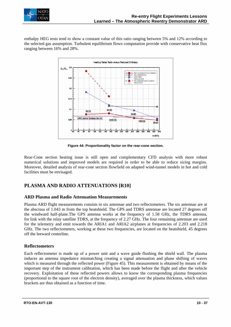
Figure 44 gives an other representation of the situation; the evolution of proportionality factor ref

F

qq 8 is

plotted versus reduced total enthalpy parameter. The figure clearly indicates that this ratio is not constant in flight, increasing with decreasing total enthalpy from 5% to 18%, whereas laminar predictions and high


RTO-EN-AVT-130 10 - 37

enthalpy HEG tests tend to show a constant value of this ratio ranging between 5% and 12% according to the selected gas assumption. Turbulent equilibrium flows computation provide with conservative heat flux ranging between 16% and 28%.

Figure 44: Proportionality factor on the rear-cone section.

Rear-Cone section heating issue is still open and complementary CFD analysis with more robust numerical solutions and improved models are required in order to be able to reduce sizing margins. Moreover, detailed analysis of rear-cone section flowfield on adapted wind-tunnel models in hot and cold facilities must be envisaged.

PLASMA AND RADIO ATTENUATIONS [R10]

ARD Plasma and Radio Attenuation Measurements Plasma ARD flight measurements consists in six antennae and two reflectometers. The six antennae are at the abscissa of 1.043 m from the top heatshield. The GPS and TDRS antennae are located 27 degrees off the windward half-plane.The GPS antenna works at the frequency of 1.58 GHz, the TDRS antenna, for link with the relay satellite TDRS, at the frequency of 2.27 GHz. The four remaining antennae are used for the telemetry and emit towards the ARIA1 and ARIA2 airplanes at frequencies of 2.203 and 2.218 GHz. The two reflectometers, working at these two frequencies, are located on the heatshield, 45 degrees off the leeward centerline.

Reflectometers Each reflectometer is made up of a power unit and a wave guide flushing the shield wall. The plasma induces an antenna impedance mismatching creating a signal attenuation and phase shifting of waves which is measured through the reflected power (Figure 45). This measurement is obtained by means of the important step of the instrument calibration, which has been made before the flight and after the vehicle recovery. Exploitation of these reflected powers allows to know the corresponding plasma frequencies (proportional to the square root of the electron density), averaged over the plasma thickness, which values brackets are thus obtained as a function of time.


10 - 38 RTO-EN-AVT-130

Γbp= Er / Ei =

Emitt

P1 P2 P3 P4

Power

anten

E

Insulat

E

Γα

PlasF F Z

Figure 45: Reflectometer Device Principle Scheme.

Results obtained from pre-flight and post-flight calibrations are presented for the reflectometer at frequency 2.218 GHz in Figure 46. As a whole, plasma frequencies have been measured between the altitudes of 100 and 42 km. But agreement between the results from the two calibrations exists only for altitudes below about 45 km. Post-flight calibration gives much higher values than the pre-flight one in the vicinity of 90 km and no solutions at intermediate altitudes. The measurements increases from the altitude of 97 km may be attributable to both the plasma apparition and the departure of a metallic plane surrounding the antenna aperture, which results in an increase in measurement uncertainty.

Figure 46: Reflectometer Measurements Restored Plasma frequency with two calibrations.


RTO-EN-AVT-130 10 - 39

TDRS, GPS and TM links For each antenna, a link budget is calculated at each time from the capsule trajectory and attitude, the antenna pattern measured before the flight and the reception system characteristics. By calculating the expected received power from these parameters and subtracting the actual received one, one restitutes the link attenuation specifically attributable to the presence of plasma. Trajectories of the capsule and of the different satellites during the reentry are visible in Figure 11. The obtained plasma attenuations for TDRS and GPS links are presented in Figure 47.

Figure 47: RF Links Attenuation time history.

From these measurements, the main conclusions are the following:

• a black-out of the forward GPS links between 92 and 28 km,

• a black-out of the backward GPS links between 87 and 41 km,

• no black-out of the TDRS link, the satellite being in backward position, but plasma attenuation between 86 and 43 km, up to -25 dB,

• a plasma attenuation of the rather backward TM ARIA1 link between 84 and 77 km,

• a black-out of the rather forward TM ARIA2 link between 70 km (beginning of recording) and 42 km.

These measurements have some coherency, with expected line of sight and signal frequency effects, that is to say lower attenuations for the backward positions and the greater frequencies.

Plasma Properties CFD Reconstruction Three-dimensional Naviers-Stokes calculations have been made at three altitudes of 85, 61.5 and 46 km, for which are available exploitable reflectometer measurements.

As can be seen on Figure 47:

• 85 km corresponds to the beginning of TDRS and GPS links attenuation measurements,

• 61.5 km is an altitude where exists the end of the plateau of TDRS link attenuation and a measurement of GPS 31 link attenuation, while other GPS links are interrupted; pyrolysis mass


10 - 40 RTO-EN-AVT-130

flow rates at this altitude are rather important and so, this altitude allows also to verify and complete injection effects observed in the preliminary study

• 46 km is in the vicinity of the end of TDRS and GPS links attenuations

Up-stream conditions and hypotheses, according to aerothermal exploitation, at these three altitudes are the following:

Altitude (km)

Angle of attack (deg)

Velocity (m/s) Hypotheses

85 19.0 7 565.6 – laminar flow – no injection – non catalytic

61.5 20.4 6 422.7 – laminar flow – with and without

injection – catalytic wall

46 21.2 3 552.5 – laminar flow – without injection – catalytic wall

Air chemistry was modelled with C. Park 1993 air chemical kinetic rates, described in reference [R12]. Additionally, relaxation times from Millikan and White for O2 and N2 relaxation of vibration, often associated to C. Park chemistry.

85 km Altitude Results (B-O Entry) As can be seen on Figure 46, the pre-flight calibration gives at this altitude, mean plasma frequencies between 1.4 GHz and 1.6 GHz, while the post-flight calibration results in much higher frequencies ranging between 7.6-20 GHz. As explained previously, the increase in plasma frequencies measured from the altitude of 97 km may be associated with the plasma apparition but also with the departure of a metallic piece surrounding the antenna which results in an increase in the measurement uncertainty. The calculated mean plasma frequency is equal to 9.1 GHz and is thus enclosed by the global measurement bracket.

At this altitude, the satellites TDRS, GPS31 and GPS14 have backward positions and the plasma attenuations are equal to -14 dB, -9 dB and -19 dB respectively. As can be seen in Figure 48, the plasma frequencies in the vicinity of the antennae are, for backward rays, close to the TDRS signal frequency and slightly greater than the GPS one.


RTO-EN-AVT-130 10 - 41

2.300E+09 1.848E+09 1.558E+091.349E+09

1.180E+09

2.300E+091.848E+09

1.558E+09

1.349E+09

1.054E+09

9.241E+08

6.261E+08

6.261E+08

9.241E+08

8.123E+08

9.241E+08

1.054E+09

1.180E+09

1.180E+09

1.054E+091.054E+09

x

z

0 2 4 6 8-7

-6

-5

-4

-3

-2

-1

0

1

2FP

2.24153E+102.04038E+101.83923E+101.63808E+101.43693E+101.23578E+101.03463E+108.33482E+096.32333E+094.31183E+092.30034E+091.84848E+091.55834E+091.34947E+091.17999E+091.05434E+099.24097E+088.12308E+086.26082E+082.88848E+08

ARD - ALTITUDE 85 KMSYMMETRY PLANE

PLASMA FREQUENCIES (Hz)

Figure 48: Plasma Frequency Distribution at 85 km altitude.

With calculated collisions frequencies that are much lower than the signals frequencies, the attenuation is highly sensitive to the plasma frequency. In such a configuration, if we rely on the computed plasma thickness, the measured attenuation allows to restore of reliable plasma frequency level. Calculations of the attenuations along the considered lines of sight give attenuations clearly greater than the observed one but, because of this high sensitivity, reductions of only a few percents for GPS 14, 20% for TDRS and 40% for GPS31 of the calculated plasma frequencies allows to obtain the observed attenuations.

So, the calculated plasma frequencies are less than 40%, greater than the ones deduced from measurements, which is within the minimal uncertainty of ± 40% affecting the calculated plasma frequencies, which corresponds to a factor 2 on the electron density.

61.5 km Altitude Results (maximum attenuation) The calculated mean plasma frequency at reflectometer position is equal to 33 GHz. Like for the higher 85 km altitude, there is a disagreement between measurements resulting from pre-flight and post-flight calibrations (see Figure 46). The pre-flight calibration results in mean plasma frequencies ranging between 2.6 and 3.8 GHz while the post-flight calibration does not yield any value.

However this plasma frequency calculated in the leeward heatshield area is enough directly related to the stagnation point value. The calculated value at this position is close to the one given by HUBERT’s abacus, which gives stagnation point plasma frequencies in function of altitude and velocity under equilibrium flow conditions. So the measurements deduced from the only available pre-flight calibration appear to be quite low and questionable.

At this altitude TDRS link and GPS31 link plasma attenuations are –18dB and –22dB respectively and both correspond to backward positions towards the capsule.

As can be seen on Figure 49, plasma frequencies clearly greater than the signal frequencies (2.27 and 1.58 GHz) are encountered along backward rays from the antennae.


10 - 42 RTO-EN-AVT-130

Figure 49: Plasma Frequency Distribution at 61.5 km altitude.

The calculated plasma attenuations along the appropriate lines of sight are much greater than the measured value and would correspond to an interrupted link. However, one can observe plasma frequencies lower than 1.58 GHz over an enough important area in the vicinity of the wall, through which the emitted signal may be much less attenuated. So the simplified used attenuation calculations may be not suitable to such a plasma configuration and a calculation (which could not be included in the study), which would take into account diffraction effects around overdense areas that could lead to attenuations much lower than the presently calculated ones.

46 km Altitude Results (B-O Exit) The plasma frequencies distribution obtained in the symmetry plane is displayed in Figure 50.

Figure 50: Plasma Frequency Distribution at 46 km altitude.

6.920E+08

5.000E+084.087E+08

2.836E+08

7.882E+07

4.087E+08

2.836E+08

1.802E+08

5.598E+085.000E+08

4.087E+08

6.920E+085.598E+08

5.000E+08

4.087E+08

2.836E+08

1.802E+08

7.882E+07

1.802E+08

4.087E+08

x

z

0 2 4 6 8 10-7

-6

-5

-4

-3

-2

-1

0

1

2FP

7.03844E+096.44404E+095.84963E+095.25523E+094.66083E+094.06642E+093.47202E+092.87762E+092.28321E+091.68881E+091.0944E+096.9204E+085.5981E+085E+084.08705E+082.83601E+081.80202E+087.88215E+07

ARD - ALTITUDE 46 KMSYMMETRY PLANE

PLASMA FREQUENCIES (Hz)

3.357E+087.416E+08

7.416E+08

4.380E+09 3.637E+09

3.357E+08

5.597E+09

4.380E+09

5.597E+09

4.927E+09

7.416E+08

7.416E+08

7.416E+08

x

z

0 2 4 6 8 10

-6

-5

-4

-3

-2

-1

0

1

2

FP4E+103.63637E+103.27275E+102.90912E+102.54549E+102.18186E+101.81824E+101.45461E+101.09098E+107.27355E+095.5971E+094.92728E+094.38002E+093.63727E+097.41593E+083.35722E+081E+06

ARD - ALTITUDE 61.5 KMCALCULATION WITHOUT INJECTION

SYMMETRY PLANEPLASMA FREQUENCIES (Hz)


RTO-EN-AVT-130 10 - 43

The measurements bracket deduced from pre-flight calibration is 1.8 – 4 GHz and the considered altitude is very close to the altitude range for which pre-flight and post-flight calibrations are in good agreement.The calculated mean plasma frequency is equal to about 2.0 GHz, if one assumes that the reflectometer does give the average plasma frequency of the turbulent flow which is likely to occur at this altitude, one can conclude to a good agreement between calculation and measurement of this parameter.

At this altitude, the TDRS satellite has a backward position and the plasma attenuation has decreased to - 4 dB. Links have been recovered with satellites GPS22, GPS03 and GPS31, corresponding respectively to positions rather forward, medium and backward and attenuations are equal to – 8 dB, – 9 dB and - 7 dB. As can be seen on Figure 50, plasma frequencies in the vicinity of the antennae are, as expected, lower than the signals frequencies but not close enough to them. This results in no plasma attenuations from the calculation instead of the few dB observed. To obtain the observed attenuations, plasma frequencies must be multiplied by factors between 2 and 3.

Given apparently faster increases in calculated attenuations with the altitude than in measured ones, these differences on plasma frequencies and attenuations may result in small differences on recovery link altitudes. For example, for GPS03 link, the calculation , based on results at 46 km and evolutions around this altitude from HUBERT’s abacus, gives the recovery value of –19 dB between about 47 and 48 km (taking into account an uncertainty factor of 2 on the electron density), while this recovery value has been observed at 49 km.

CONCLUDING REMARKS

As far as aerothermodynamic issue is concerned, ARD Post-Flight analysis task funded by ESA/ESTEC was an unique opportunity to assess our prediction capabilities for such re-entry vehicle that in spite of its similitude with a simple axisymetrical Apollo shape, was found to be rather complex to identify; its large bluntness resulting in a large subsonic zone that was found to induce some numerical convergence difficulties, and to require specific mesh grid generation strategy. Also because of its bluntness, flow-field effects generated by some specific phenomena like real gas effects on the front-shield were difficult to detect or measure accurately.

Real gas effects have been found to be significant during all the hypersonic part of re-entry down to Mach 8. This was identified at least by 2 or 3 kinds of measurements, namely the front-shield surface pressure measurements, the trim incidence reconstruction and possibly the restored heat flux. This was confirmed by CFD analysis with non equilibrium or equilibrium Air assumptions. Real gas effects were found to mark the front-shield section pressure distribution by magnifying the flow expansion on the leeward part while increasing the compression near the stagnation point and shifting this point towards the shoulder. A real gas effects marker has been defined thanks to this observation. It is also remarkable that the trend given by this marker was reproduced by the European high-enthalpy HEG and F4 facilities, showing these facilities to have capabilities to simulate flight phenomena. This kind of markers can be generalized for preparation of future experimental vehicle for any flow phenomena to be investigated. Instead of basing the identification on a single type of measurements, a combination of measurements should be looked for, for maximizing the flight experiment return.

The preflight AEDB underestimated the real gas effects in the whole hypersonic range: at very high Mach numbers (M > 24) where APOLLO derived effects appeared too low, and at low Mach numbers (M =10) where an inappropriate perfect gas assumption was retained.

The flight analysis pointed out the need for a good knowledge of the vehicle characteristics, before and during the flight: ARD uncertainties led to some difficulties for the observability of physical phenomena such as real gas effects.


10 - 44 RTO-EN-AVT-130

The analysis highlighted the good consistency between all available data. The preflight AEDB is validated for these force coefficients (CA ; CN), even if no real gas effect was taken into account, because of the rather conservative uncertainties.

The numerical simulations are coherent with the flight reconstruction trends; they show some real gas effects, especially on CA, in high hypersonic range (M > 10); results are rather insensitive to viscous / inviscid assumptions.

The flight analysis pointed out the need for improved atmospheric characterisation, required for accurate aerodynamic coefficient reconstruction.

Aerothermal environment characterization was difficult to address because of a premature failure of some thermocouples and due to uncertainties in the flight heat flux restoration from temperature measurements that were strongly connected to the degradable TPS materials properties knowledge. An inverse procedure that account for material out-gassing and recession has been successfully developed during this post-flight analysis providing with some promising results that could easily be used in others applications including degadable materials (Mars entries, TPS materials ground tests exploitation, measurement devices development,…).

It was also found that a quite early laminar-to-turbulent transition occurred on the front-shield leeward side around ReD=5 105, that a maximum heating rate of roughly 1.2 MW/m2 occurred on the shoulder windward centerline and that this maximum heating rate is affected by so-called real gas effects. On the rear-cone, the flow remained attached on the windward side, heat fluxes were found to be lower than expected but higher than pure laminar prediction; a possible transitional flow regime might have occurred in this region resulting in heating ranging between laminar lower bound and turbulent upper bound.

Black-out region was reasonably predicted using C. Park chemistry with Milikan-White relaxation times for N2 and O2 molecules. However, reflectometer devices performances need to be improved in order to discriminate plasma frequency, collision frequency and plasma thickness. Multi-frequency reflectometers might be developed in the future in order to addresss this issue. Attenuations were found to be highly sensititive to the antennae relative position w.r.t. receivors. In particular, TDRS experienced no full attenuations that might be useful for future re-entry missions.

The successful ARD flight brought a lot of high quality aerodynamic information that allowed to improve our knowledge about prediction tools capability. Both CFD and ground facilities were found to be adequate if mastered, for describing main flow phenomena that drive the design and the performances of a guided re-entry capsule. These prediction tools will be used extensively in future reentry projects.

ARD was the very first guided re-entry vehicle experienced in West Europe. Post-flight data show that the ARD flight was a great success. All flight data have been recorded or transmitted by telemetry to ARIA airplanes. All demonstration and system requirements have been met, in particular trajectory and flight control were close to nominal, the DRS sequences have been successfully deployed; the capsule sea-landed by 3 km off its expected landing point and was recovered by the French Navy for expertise.

The vehicle is now presented in the ESTEC Space Exhibition in Noordwijk (The Netherlands).

AKNOWLEDGEMENTS

Special thanks to ESA / ESTEC as the customer that rendered possible this re-entry demonstration. The author would also like to thank all the EADS-ST teams and partners (SABCA, SONACA, Alénia, EADS Astrium, ETCA, TRASYS), the partners who contributed to post-flight analysis tasks (VKI, ESTEC, CFS, DLR, ONERA, Alénia) and the EADS-ST people who participated to the post-flight


RTO-EN-AVT-130 10 - 45

analysis tasks and who contributed to the present paper: J.L. Macret, Y. Veronneau, S. Riccardi, J.Y. Rolland, L. Bouaziz, J.F. Pallegoix, J. Collinet.

REFERENCES

[R1] Rolland J.Y., “Atmospheric Reentry Demonstrator : Flight Control Post-Flight Restitution”, AAAF 2nd International Symposium – Atmospheric Reentry Vehicles and Systems, Arcachon, March 26-29, 2001.

[R2] Pignié G., Bouaziz L., Kebci H., Trinquard F., “Parachutes Opening Triggering Algorithm of the Atmospheric Re-entry Demonstrator”, AAAF 1st International Symposium – Atmospheric Reentry Vehicles and Systems, Arcachon, March 16-18, 1999.

[R3] Paulat J.C., “MSTP Aero Tools-Synthesis of critical points”, HT-SF-WP1130-087-AS, January 1997.

[R4] Veronneau Y., “Atmospheric Reentry Demonstrator : Post Flight Analysis – Surface Pressure”, AAAF 2nd International Symposium – Atmospheric Reentry Vehicles and Systems, Arcachon, March 26-29, 2001.

[R5] Paulat J.C., “Atmospheric Reentry Demonstrator : Post-Flight Analysis – Aerodynamics”, AAAF International Symposium – Atmospheric Reentry Vehicles and Systems, Arcachon, March 26-29, 2001.

[R6] Tran P., “Atmospheric Reentry Demonstrator : Post-Flight Analysis – Aerothermal Environment”, AAAF International Symposium – Atmospheric Reentry Vehicles and Systems, Arcachon, March 26-29, 2001.

[R7] Vincent P., “Ariane 5: Ambiance thermique – procédure d’exploitation des fluxmètres vol”, EADS-ST Technical Note A5-NT-A-1-2093-ASAI, January, 1998.

[R8] Tran Ph., Baillion M. “Atmospheric Reentry Demonstrator Aerothermodynamic Justification File”, EADS-ST Technical Note, HT-JF-B-01-AS/M, February, 1995.

[R9] Estebe B., “ARD Post-Flight Analysis WP23400 – ARD flight convective heat flux derived from calorimeters”, EADS-ST Technical Note HT-TN-0-04-AS/M, December, 1999.

[R10] Pallegoix J.F., “Atmospheric Reentry Demonstrator : Post Flight Analysis – Flight Rebuilding with CFD”, AAAF 2nd International Symposium – Atmospheric Reentry Vehicles and Systems, Arcachon, March 26-29, 2001.

[R11] Boukhobza P., Riccardi S., Walpot L., “Atmospheric Reentry Demonstrator : Post Flight Analysis – Plasma and Radio Attenuations Exploitation”, AAAF 2nd International Symposium – Atmospheric Reentry Vehicles and Systems, Arcachon, March 26-29, 2001.

[R12] Park C., “Review of chemical-kinetics problems of future NASA missions – I: Erath entries”, Journal of Spacecraft and Heat Transfer Vol. 7, n° 3, July-September 1993.


10 - 46 RTO-EN-AVT-130

re-entry flight experiments lessons learned – the ... · re-entry flight experiments lessons...

Documents