The claim is bond, GDP-indexed bond

The non-contingency puzzle: limitations to sovereign risk-sharing

Antoine Levy

June 2016

Supervisors: Prof. Daniel Cohen and Prof. Pierre-Olivier Gourinchas

Referee: Prof. Jean Imbs

Masters thesis

Analysis and Policy in Economics

ÉCOLE NORMALE

S U P É R I E U R E

Paris School of Economics UC Berkeley Ecole Normale Supérieure

JEL codes: H63, F34, E62, G12

Keywords: sovereign debt, insurance, default risk, indexation

Acknowledgements

I am grateful to my advisors, Prof. Daniel Cohen and Prof. Pierre-Olivier Gourinchas, for agreeing

to supervise this masters thesis, and for their invaluable advice and suggestions. I also thank Prof.

Jean Imbs for agreeing to referee it, and for his support of my application to the Berkeley exchange

program; and Prof. Ricardo Caballero, whose remarks on pricing kernels and central bank reserves

management, during a conversation in Cambridge, were illuminating.

I thank my sovereign-debt-obsessed but nonetheless outstanding friends Paul-Adrien Hyppolite,

Thomas Lambert, and especially Thomas Moatti for our discussions about Greece and Ukraine, for

suggesting the AMECO database, and for providing the Greek prospectus and Bloomberg data. I

also owe (non-contingent) debts and drinks to Julien Acalin, Zach Bleemer, Sebastian Camarero

Garcia, Charles Murciano, and Charles Serfaty, for their useful and friendly insights on this topic.

I am grateful to my fellow Californian traveller Louise Guillouët for her unwavering patience and

support during the writing of this thesis, and for the daily intake of - Philz - coffee she agreed to

enjoy with me.

I acknowledge the financial support of the American Foundation for the Paris School of Economics

during my semester at UC Berkeley, and the Ecole Normale Supérieure during my semester at the

Paris School of Economics.

Needless to say, all remaining mistakes in this work are my responsibility alone.

Paris, June 5, 2016.

Abstract

State-contingent sovereign liabilities are widely considered an optimal way of linking a country’s

debt service to its ability-to-pay, by making repayment obligations depend on the underlying state

of the economy. However, their use in practice has remained limited. To account for this "non-

contingency puzzle", I intend to better characterize the constraints faced by the sovereign issuing

such instruments. Imperfect information may lead to partial insurance; limited commitment adds

incentive compatibility restrictions; and investor risk-aversion, model uncertainty and pricing diffi-

culties may make such instruments too costly to be relevant quantitatively.

The objective is to provide a qualitative and quantitative evaluation of how much risk the sovereign

can "afford to share" via equity-like instruments. The thesis proceeds in four sections. First, we

provide micro-foundations for partially indexed debt, via an optimal contracting problem, to char-

acterize information and commitment imperfections preventing full risk-sharing. Armed with such

justifications for "S-shaped" insurance, we then proceed with an asset pricing exercise, simulating

paths for GDP and indexed debt, to quantitatively gauge the importance of investor risk-aversion

and model mis-specification for various indexation formulas. In order to combine the previous

insights in a consistent framework when both indexed and non-contingent debt are available, we

turn to a general equilibrium model of sovereign default with indexed and non-contingent debt and

risk-averse lenders, and quantitatively calibrate the model to the Greek economy. Finally, we fo-

cus on post-default negotiations, and justify why indexed debt may then be considered an optimal

restructuring mechanism.

Contents

Introduction 4

The non-contingency puzzle . . . . . . . . . . . . . . . . . . . . . . . . . . . . . . . . . . . 4

Indexed debt: an old idea . . . . . . . . . . . . . . . . . . . . . . . . . . . . . . . . . . . . 5

Benefits of indexed sovereign debt . . . . . . . . . . . . . . . . . . . . . . . . . . . . . . . 6

From Greece with love: a short motivation . . . . . . . . . . . . . . . . . . . . . . . . . . . 8

1 For your eyes only: Optimal indexation under imperfect information 12

1.1 Justifications for non-contingency . . . . . . . . . . . . . . . . . . . . . . . . . . . . . 12

1.2 Constrained optimal contracts . . . . . . . . . . . . . . . . . . . . . . . . . . . . . . . 14

1.2.1 Insurance and the value of imperfect signals . . . . . . . . . . . . . . . . . . . 15

1.2.2 Contingency via default, or contingency via imperfect indexation . . . . . . . 18

1.2.3 Unobservable states . . . . . . . . . . . . . . . . . . . . . . . . . . . . . . . . 22

1.3 Incentive compatible sovereign debt with incomplete information . . . . . . . . . . . 24

1.3.1 First-best benchmark . . . . . . . . . . . . . . . . . . . . . . . . . . . . . . . . 25

1.3.2 Full information, imperfect commitment . . . . . . . . . . . . . . . . . . . . . 26

1.3.3 Asymmetric information, imperfect commitment . . . . . . . . . . . . . . . . 28

1.4 The indexed debt contract . . . . . . . . . . . . . . . . . . . . . . . . . . . . . . . . . 34

1.4.1 Discussion . . . . . . . . . . . . . . . . . . . . . . . . . . . . . . . . . . . . . . 35

2 Casino Royale: A Monte-Carlo asset-pricing exercise 38

2.1 Past attempts at pricing GDP-indexed instruments . . . . . . . . . . . . . . . . . . . 39

2.2 The role of the indexation formula . . . . . . . . . . . . . . . . . . . . . . . . . . . . 41

2.2.1 Existing designs for GDP-indexed debt . . . . . . . . . . . . . . . . . . . . . . 41

1

2.2.2 Classification of indexation formulas . . . . . . . . . . . . . . . . . . . . . . . 43

2.3 The role of output statistical properties . . . . . . . . . . . . . . . . . . . . . . . . . 44

2.3.1 The risk of model mis-specification . . . . . . . . . . . . . . . . . . . . . . . . 44

2.3.2 Persistence and volatility . . . . . . . . . . . . . . . . . . . . . . . . . . . . . 45

2.4 The role of investor risk-aversion . . . . . . . . . . . . . . . . . . . . . . . . . . . . . 46

2.4.1 The world is not enough: growth correlations . . . . . . . . . . . . . . . . . . 46

2.4.2 A toy model of risk-averse investors . . . . . . . . . . . . . . . . . . . . . . . . 47

2.5 Simulations . . . . . . . . . . . . . . . . . . . . . . . . . . . . . . . . . . . . . . . . . 48

2.5.1 Indexation formulas used in our simulations . . . . . . . . . . . . . . . . . . . 48

2.5.2 Output process used in the simulations . . . . . . . . . . . . . . . . . . . . . . 49

2.5.3 Pricing kernel used in the simulations . . . . . . . . . . . . . . . . . . . . . . 50

2.5.4 Methodology and results . . . . . . . . . . . . . . . . . . . . . . . . . . . . . . 51

3 You only live twice: Recursive general equilibrium models of indexed debt 61

3.1 Preliminary reflections on default with indexed debt . . . . . . . . . . . . . . . . . . 62

3.2 A general equilibrium model with exogenous output . . . . . . . . . . . . . . . . . . 63

3.2.1 The environment . . . . . . . . . . . . . . . . . . . . . . . . . . . . . . . . . . 64

3.2.2 The government’s decision . . . . . . . . . . . . . . . . . . . . . . . . . . . . . 65

3.2.3 Some analytical results on the borrower side . . . . . . . . . . . . . . . . . . . 65

3.2.4 The lenders’ problem . . . . . . . . . . . . . . . . . . . . . . . . . . . . . . . . 67

3.2.5 Definition of equilibrium . . . . . . . . . . . . . . . . . . . . . . . . . . . . . . 70

3.2.6 Optimal debt structure . . . . . . . . . . . . . . . . . . . . . . . . . . . . . . . 70

3.3 Calibration and implementation of the algorithm . . . . . . . . . . . . . . . . . . . . 74

3.3.1 A detrended version . . . . . . . . . . . . . . . . . . . . . . . . . . . . . . . . 74

3.3.2 Calibration and parametrization . . . . . . . . . . . . . . . . . . . . . . . . . 75

3.3.3 Fixed exogenous shares of debt . . . . . . . . . . . . . . . . . . . . . . . . . . 76

3.3.4 Endogenous shares of debt . . . . . . . . . . . . . . . . . . . . . . . . . . . . . 79

4 Die another day: GDP-indexation after default 87

4.1 Financing, forgiving, or indexing a debt overhang? . . . . . . . . . . . . . . . . . . . 88

4.1.1 Legacy debt and indexation . . . . . . . . . . . . . . . . . . . . . . . . . . . . 88

2

4.1.2 The benefits of indexation . . . . . . . . . . . . . . . . . . . . . . . . . . . . . 93

4.2 Market access and the unit root: how persistent are drops in output? . . . . . . . . . 95

4.2.1 A market for sovereign lemons? . . . . . . . . . . . . . . . . . . . . . . . . . . 96

4.2.2 Quantum of solace: indexed debt in bad times . . . . . . . . . . . . . . . . . . 98

Concluding remarks 100

Bibliography 102

Appendices 108

3

Introduction

The non-contingency puzzle

Despite the absence of enforcement mechanisms or bankruptcy frameworks at the supranational level,

sovereigns overwhelmingly tend to pay back their debts, and investors continue to lend to them. Various

explanations have been proposed for this puzzling observation. They range from the sovereign’s reputation

concerns (Eaton and Gersovitz 1981) or political economy justifications (Cuadra and Sapriza 2008), to the

fear of direct sanctions (Bulow and Rogoff 1989), the costs to the private sector of losing market access

(Mendoza and V. Yue 2012), or even to "rational Ponzi schemes" behaviour (Rochet 2006).

However, given that market access is at all available, a new puzzle emerges. Most representations of sovereign

debt assume not only impatient, but also risk-averse, borrowers, to justify borrowing from international mar-

kets in the first place. It should follow that these sovereigns have an interest in issuing state-contingent debt

to diversify away their income stream risk. Since debtors are able to convince investors to lend to them

despite imperfect commitment, why is sovereign borrowing not more contingent on income risk? Otherwise

said, why is there no, or so little, "sovereign equity"(Park and Samples 2016)?

In a famous Harvard Business Review article, Paul Krugman (Krugman 1996) once asserted that “a country

is not a company”. Although Krugman was referring to the "unhealthy" obsession with competitiveness,

the incompleteness of sovereign finance instruments (Barro 1995), when compared to securities issued by

private entities, is another major contrast between sovereign states and corporations. While sovereigns issue

bonds, akin to senior corporate debt securities, and take on syndicated bank loans, there is no sovereign

equivalent of equity, a contingent asset with a riskier payoff structure, and a higher correlation with economic

performance. We label this fact the non-contingency puzzle.

Default risk and income risk Sovereign borrowers face uncertainty in their ability to repay their

liabilities. For distressed economies, repaying debt in "bad times" entails high costs, since it corresponds to

sub-optimal transfers of resources from states with high marginal utility of consumption, to low marginal

utility of consumption states (M. Aguiar and Amador 2013): as an illustration, one can think of forced

4

pro-cyclical fiscal consolidation in times of crisis. Default does allow for a crude form of contingency, but it

tends to be a last resort solution, due to its aforementioned costs in terms of output disruption and market

access.

Many researchers, and many more policy makers (Griffith-Jones and Sharma 2006, Borensztein and Mauro

2002, among others), have thus suggested that sovereign liabilities should be indexed to variables highly

correlated with a sovereign’s ability-to-pay, such as commodity exports prices, gross domestic product, or

tax revenues. Conversely, it has been suggested that emerging sovereigns invest part of their assets in globally

traded securities with payoffs highly correlated with their own marginal utility of resources (Caballero and

Panageas 2004). While academics and policy makers have lamented the absence of such growth-hedging

instruments, it has been difficult to identify precisely what factors may prevent their emergence.

Indexed debt: an old idea

Historically, some sovereign borrowers did take on debt with contingent repayments terms. Philip II of Spain

issued de facto contingent bonds to Genoan bankers, with repayment implicitly or explicitly dependent on

certain events’ occurring characterizing a “good” state of the world, such as the arrival of cargoes of sil-

vers from the New World (Mauricio Drelichman and Hans-Joachim Voth 2013). One may argue that the

most-well known historical example of government equity is in fact the "Law System", a scheme devised

by Controller-General of the Finances of the Kingdom of France John Law, in 1717-20, to swap most of

France’s sovereign debt outstanding for equity shares in the "Compagnie perpétuelle des Indes", or - as it is

sometimes known after one of its subsidiaries - the "Mississippi Company", a large conglomerate with income

essentially made up from proceeds from French North America ("Louisiana") activities, farmed taxes and

other leased revenues (see Velde 2007 for a detailed account and assessment of the Law system as an example

of "government equity").

However, at odds with the theoretical advantages of state-contingent debt, sovereign borrowing in practice

is mostly non-contingent. Once they incur debt obligations, sovereigns are forced to fulfill them entirely, in

nominal terms, or to default, with associated costs in terms of reputation, trade and output disruptions, and

financial sanctions. Moreover, when, on rare occasions, contingent sovereign liabilities are issued, it is not

as part of an ex ante "optimal risk-sharing strategy", but more frequently ex post, to improve renegotiation

offers to creditors in the aftermath of debt restructurings. The stated goal is then to offer potential for value

recovery to investors affected by haircuts, mimicking the “debt-equity swaps” that are frequent in corporate

bankruptcy. The cases of Argentina (2001), Greece (2011-12), or Ukraine (2015) issuing GDP warrants

are the most well-known; but such instruments have also been used during the “Brady” restructurings of

sovereign debt, most notably by Costa Rica, Bosnia and Bulgaria, under the label “Value Recovery Rights”

5

(Griffith-Jones and Sharma 2006).

The quantitative literature on defaultable sovereign debt has studied extensively the incentives to default un-

der non-credible commitment and enforceable penalties, and the limits they imply on borrowing by sovereign

states (see e.g. M. Aguiar and Gopinath 2006; Arellano 2008). Some researchers have since attempted to

introduce indexed-bonds in such a framework, with a view to quantify the welfare gains achieved via two

channels: a reduced probability of default, on the one hand (see Hatchondo and Martinez 2012 and Faria

2007); and a higher borrowing upper limit resulting in better consumption smoothing, on the other hand

(see in particular Sandleris, Saprizza, and Taddei 2011). Another strand of literature has looked more empir-

ically into the smoothing potential of indexing debt to GDP, either by running counter-factual simulations

(Borensztein and Mauro 2002; Sandleris and M. Wright 2013), or by making ad hoc assumptions on fiscal

feedbacks effects (Barr, Bush, and Pienkowski 2014).

Benefits of indexed sovereign debt

The risk-sharing benefits of sovereign equity securities could be approximated by “GDP-linked bonds”, i.e.

sovereign debt providing equity-like exposure to a country’s macroeconomic outcomes for the holder, and

equity-like insurance for the issuer, via state-contingent payments (non-decreasing in the state of the econ-

omy). In general terms, they are defined by an upside when a country “does well” in terms of its aggregate

income, but lower returns when GDP is below its expected trend. A number of benefits of linking debt ser-

vice to GDP are listed below, ranked from the most explored in the literature to the least documented effects.

1. Reduction in default risk - It has been frequently observed that GDP-linked securities reduce

default risk (and the associated spillover costs in terms of output and employment losses), by lowering

the debt service burden in recession times, during which a large majority of debt restructurings occur

(Hatchondo and Martinez 2012, Sandleris, Saprizza, and Taddei 2011).

2. Higher borrowing capacity - The default risk reduction entails, in turn, that issuing GDP-indexed

bonds may increase the debt threshold a country can safely reach without jeopardizing solvency (Barr,

Bush, and Pienkowski 2014).

3. Counter-cyclical fiscal policy in busts - GDP-indexed bonds can ease the implementation of

counter-cyclical fiscal policy, by freeing up fiscal space in bad times. By reducing the need to run

primary surpluses during busts, they can avoid the risks of an “austerity spiral”, where a government

has to tighten fiscal policy to meet rising interest service, thus endogenously stifling economic activity

and further increasing default risk (Borensztein, M. Chamon, et al. 2004). In the case of multiple

6

equilibria for solvent but illiquid countries (Cole and Kehoe 2000), it could avoid negative debt spirals

where higher interest rates themselves jeopardize solvency (Marcus Miller and Lei Zhang 2012).

4. Macroeconomic stabilization during booms - Conversely, rising debt payments during booms

would discipline government expenditures (or force governments to raise taxes) and avoid overheat-

ing: GDP-linked securities would act as automatic stabilizers by smoothing debt payments along

the business cycle (Borensztein, M. Chamon, et al. 2004) and offer a credible commitment to sound

macroeconomic policies, notably in currency unions where fiscal commitment can be weak (Mark

Aguiar et al. 2014).

5. Diversification and hedging of systemic risks -These bonds could also be used by individuals, or

specific institutions (pension funds, re-insurers), to diversify “macroeconomic risk” away, by shorting

an “equity stake” in their home country’s aggregate income, and taking a long position in foreign GDP-

indexed securities (Athanasoulis, Shiller, and Wincoop 1999) with low or no correlation to their own

income. Simulations on risk-pooling among groupings of countries with uncorrelated growth outcomes

show the welfare gains of such growth risk-sharing could potentially be large (Callen, Imbs, and Mauro

2015).

6. Improved debt restructuring framework - Equity-like sovereign securities would introduce an

order of seniority among a country’s creditors: this would be appealing to those calling for a more

efficient and structured sovereign debt restructuring framework (Park and Samples 2016). Here, a

parallel should be made with various proposals for orderly debt restructuring in the euro area, such

as the “blue bond proposal” (Von Weizsäcker and Delpla 2010), essentially another contingent-debt

proposal to replicate a hierarchy of burden-sharing among creditors depending on growth outcomes.

7. Information extraction and nominal GDP targeting - Such securities would also allow markets

to extract signals on agents’ expectations for the path of domestic product, and give private agents

incentives to develop accurate forecasts, a useful information for central banks in the conduct of mone-

tary policy. In that respect, they would provide policymakers and market players with “market-implied

GDP expectations”. In the same way inflation-targeting central banks have paid close attention to

inflation-linked bonds (e.g. TIPS in the US, inflation gilts in the UK, OATi in France), nominal GDP-

targeting authorities would benefit from the introduction of GDP-linked bonds both for information

and intervention purposes1. As recommended by “market monetarists” (see e.g. Sumner 2006), mone-

tary authorities could intervene on this market to adapt the monetary base to changes in expectations

of the path of nominal GDP.1GDP-linked bonds, another whole literature to synthetize into market monetarism, blog post on

www.marketmonetarist.com

7

From Greece with love: a short motivation

A simple illustration of such benefits may be gathered from the Greek experience. To provide suggestive

evidence on the counter-factual impact that indexing a given share of Greece’s debt to GDP would have had

on debt service before and during the crisis, we quantify to what extent the trajectory of debt could have

been smoothed when output dropped during the crisis.

We plot in figure 1 the trajectory of Greece’s primary and general government deficit from 1995 to 2015. The

data were retrieved from the European Commission’s AMECO database, and cross-checked with the IMF’s

Government Finance Statistics. We first reconstructed a series for the implied interest service expenditure

from the difference between the general and primary deficit. To obtain the implied interest rate on Greek

Figure 1: Greek general government primary surplus and general deficit

debt, one has to practice a number of so-called "stock-flow" adjustments, notably to account for the 2012

restructuring and for the pre-2000 variations in exchange rates between the euro and the drachma. The

interest service expenditure (the difference between the general and the primary deficit, see fig.2), once

divided by the stock of government debt, provides us with an implicit nominal interest rate of debt (see

fig.3), which, as is well known, has been steadily declining since the beginning of the 1990’s, mainly because

Greece’s inflation levels were brought down, and the country was treated as part of the core Eurozone by

international debt markets (and, as such, benefited from low nominal interest rates in spite of its rising

government debt). One can note that after 2012, most of the debt outstanding was held by official creditors

and bore even lower interest charges.

We plot below the relative paths of the implied real interest rate on government debt and the real growth

rate for Greece (see fig.4). One can observe a negative correlation of −0.25. We define a simple indexation

formula rINDt = αgt such that on average, E(rIND) = E(r) with r the implied real interest rate inferred from

8

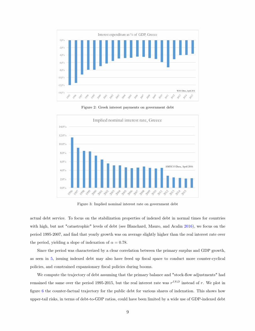
Figure 2: Greek interest payments on government debt

Figure 3: Implied nominal interest rate on government debt

actual debt service. To focus on the stabilization properties of indexed debt in normal times for countries

with high, but not "catastrophic" levels of debt (see Blanchard, Mauro, and Acalin 2016), we focus on the

period 1995-2007, and find that yearly growth was on average slightly higher than the real interest rate over

the period, yielding a slope of indexation of α = 0.78.

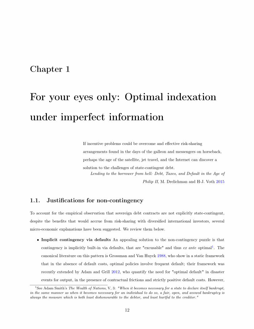
Since the period was characterized by a clear correlation between the primary surplus and GDP growth,

as seen in 5, issuing indexed debt may also have freed up fiscal space to conduct more counter-cyclical

policies, and constrained expansionary fiscal policies during booms.

We compute the trajectory of debt assuming that the primary balance and "stock-flow adjustments" had

remained the same over the period 1995-2015, but the real interest rate was rIND instead of r. We plot in

figure 6 the counter-factual trajectory for the public debt for various shares of indexation. This shows how

upper-tail risks, in terms of debt-to-GDP ratios, could have been limited by a wide use of GDP-indexed debt

9

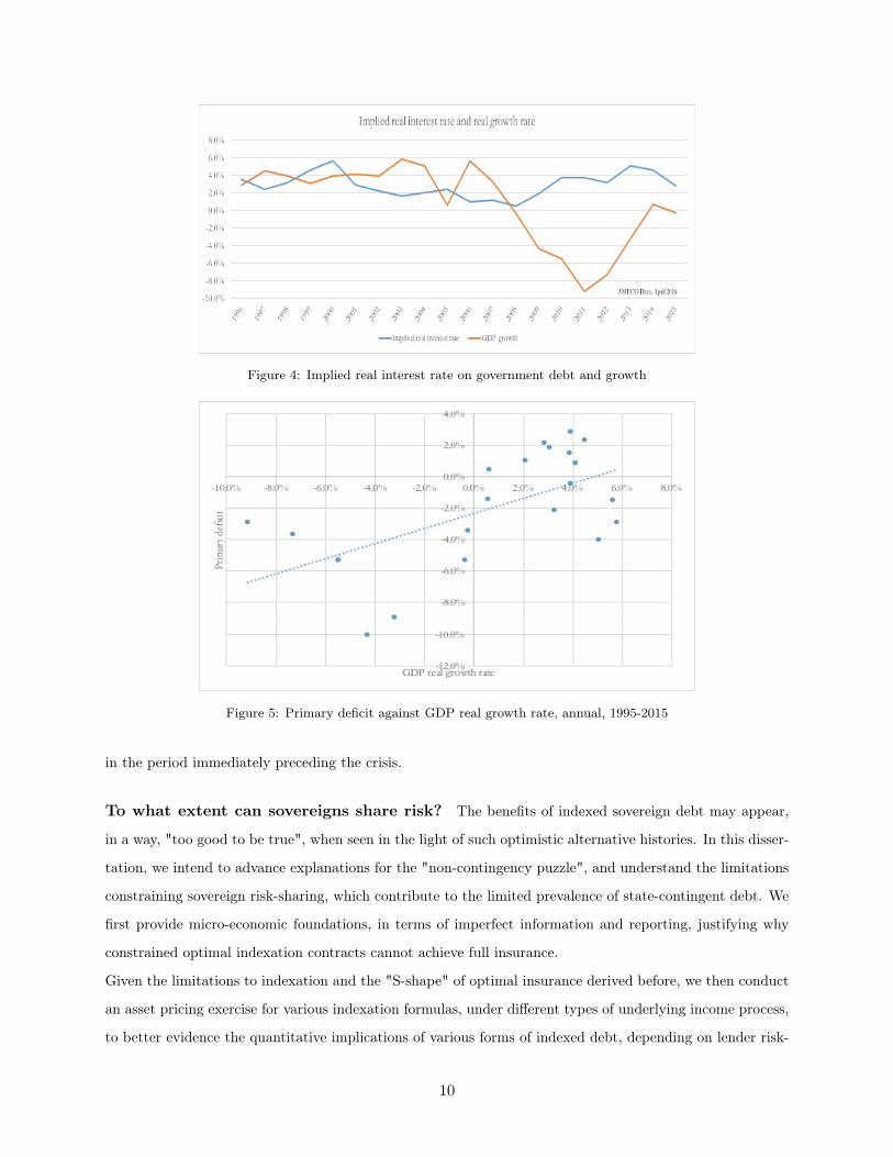
Figure 4: Implied real interest rate on government debt and growth

Figure 5: Primary deficit against GDP real growth rate, annual, 1995-2015

in the period immediately preceding the crisis.

To what extent can sovereigns share risk? The benefits of indexed sovereign debt may appear,

in a way, "too good to be true", when seen in the light of such optimistic alternative histories. In this disser-

tation, we intend to advance explanations for the "non-contingency puzzle", and understand the limitations

constraining sovereign risk-sharing, which contribute to the limited prevalence of state-contingent debt. We

first provide micro-economic foundations, in terms of imperfect information and reporting, justifying why

constrained optimal indexation contracts cannot achieve full insurance.

Given the limitations to indexation and the "S-shape" of optimal insurance derived before, we then conduct

an asset pricing exercise for various indexation formulas, under different types of underlying income process,

to better evidence the quantitative implications of various forms of indexed debt, depending on lender risk-

10

Figure 6: Alternative paths for Greek government debt

aversion and output process specification.

To contextualize our results in a broader framework, we go on to develop a general equilibrium model of

indexed and non-contingent debt with default risk. Calibrating the model on Greek data, we show that when

facing risk-averse investors, even with access to indexed debt, the sovereign will prefer to issue a mix of debt

and "equity", rather than fully transfer income risk to foreign investors.

Finally, we focus on the empirical observation that indexed debt has most often been used in post-default

episodes, and provide theoretical justifications why it may indeed represent the optimal window of opportu-

nity to issue such instruments, as an optimal renegotiation mechanism.

11

Chapter 1

For your eyes only: Optimal indexation

under imperfect information

If incentive problems could be overcome and effective risk-sharing

arrangements found in the days of the galleon and messengers on horseback,

perhaps the age of the satellite, jet travel, and the Internet can discover a

solution to the challenges of state-contingent debt.Lending to the borrower from hell: Debt, Taxes, and Default in the Age of

Philip II, M. Drelichman and H-J. Voth 2015

1.1. Justifications for non-contingency

To account for the empirical observation that sovereign debt contracts are not explicitly state-contingent,

despite the benefits that would accrue from risk-sharing with diversified international investors, several

micro-economic explanations have been suggested. We review them below.

• Implicit contingency via defaults An appealing solution to the non-contingency puzzle is that

contingency is implicitly built-in via defaults, that are "excusable" and thus ex ante optimal1. The

canonical literature on this pattern is Grossman and Van Huyck 1988, who show in a static framework

that in the absence of default costs, optimal policies involve frequent default; their framework was

recently extended by Adam and Grill 2012, who quantify the need for "optimal default" in disaster

events for output, in the presence of contractual frictions and strictly positive default costs. However,

1See Adam Smith’s The Wealth of Nations, V, 3: "When it becomes necessary for a state to declare itself bankrupt,in the same manner as when it becomes necessary for an individual to do so, a fair, open, and avowed bankruptcy isalways the measure which is both least dishonourable to the debtor, and least hurtful to the creditor."

12

given the magnitude of disruptions associated with sovereign defaults, contractual frictions would have

to be large enough to justify not writing even imperfect explicitly state-dependent contracts.

• Moral hazard Another hypothesis is that state-contingent contracts are highly subject to misre-

porting by governments - who are also the main providers of macroeconomic data. More generally,

moral hazard problems, because the sovereign lacks commitment to implement the first-best growth-

enhancing policy (Krugman 1988), may make state-contingent contracts difficult to implement. How-

ever, given that reporting high growth is often viewed as a goal of even opportunistic governments,

the incentives to under-report would need to be significant to counteract this effect.

• Investor risk aversion One answer (see e.g. Pina 2015) is that if investors are highly risk-averse, the

cost of issuing state-contingent contracts may outweigh the benefits, because the demand for indexed

debt will be more inelastic, enabling creditors to capture a higher share of the surplus from financing.

More generally, the volatility in payoffs associated with contingency may outweigh the benefits of

insurance, even for the borrower, if, for example, interest rates are subject to random shocks (Durdu

2009).

• Costly state verification An alternative explanation is that perfect contingency is not optimal in

the presence of informational frictions, in the spirit of the costly state verification (CSV) literature

(Townsend 1979). The paper by Bersem 2012 on incentive-compatible sovereign debt applies this

strand of research to sovereign debt, suggesting enforcement problems may contradict the optimality of

the "standard debt contract". However, realized incomes may be more easily observable for sovereigns

than for private agents, as will be discussed later on.

• Commitment problems in good states Another key explanation is that the sovereign cannot

commit to higher repayment schedules in good states (Kehoe and Levine 1993), thus making it more

difficult to meet the investor’s participation constraint, especially if a limited liability constraint binds

in bad states.

• Market structure Finally, some justifications focus on regulatory or institutional features of fixed-

income markets that prevent investors in sovereign debt from taking an equity-like position in sovereign

finance, or that would make the pricing of such instruments difficult. "Novelty premia" (Marcos

Chamon, Costa, and Ricci 2008), or a lack of liquidity in GDP-indexed bond markets (Blanchard,

Mauro, and Acalin 2016) have been mentioned as examples of such limitations.

13

1.2. Constrained optimal contracts

It is almost tautological to assert that an optimal financing contract between risk averse borrowers and risk-

neutral lenders, in a first-best world, should entail full insurance, i.e. constant consumption. The sovereign

would pay (beyond the required risk-free return) the difference between output and its expected value when

output is above its mean, receive that difference when output is below the mean, and thus ensure a constant

consumption stream, while respecting the lender’s zero-profit participation condition.

However, no such contracts are observed in reality. We consider in this chapter three main constraints which

may prevent full insurance:

• imperfect commitment by the sovereign, who could always prefer to repudiate its liabilities. This

willingness to pay constraint is specific to sovereigns, given that private agents can be forced to enter

ordered bankruptcy frameworks, and thus full recovery of existing assets can be achieved.

• imperfect information on the sovereign’s true ability to pay, thus leading to informational rents. This

constraint, on the contrary, is probably less binding for sovereigns than for private borrowers, given

the amount of public information (or proxies) available on a sovereign’s true capacity to pay. Such

proxies are a key element of our definition of optimal financing contracts in this section.

• limited liability constraints for the investor, which make additional payments to the sovereign in bad

times difficult to implement. In other words, sovereign debt markets are characterized by a two-stage

game, a financing period where the investor makes payments to the sovereign, and a repayment stage

when the flow of funds is reversed. We take that structure as given, although it could be envisaged that

"insurers" rather than bondholders commit to paying the sovereign money in bad times. Liquidity in

indexed bond markets is likely to require such a limited liability clause in practice, stating that the

investor cannot be called upon to make additional payments to the sovereign.

A constrained optimal debt contract for sovereign borrowers, loosely speaking, maximizes the amount of

insurance (which can be thought of as the region of states where consumption is constant and thus repayment

rises one-for-one with income), while respecting the above constraints. We intend to show that such a contract

can be viewed as an optimal "sovereign debt-equity mix", or, alternatively, as an S-shaped contract (a "bull

spread") which closely resembles existing proposals for GDP-indexed debt.

This section relates to the reflection on "incentive-compatible sovereign debt". As in Bersem 2012, the

optimal sovereign debt contract differs from Gale and Hellwig 1985’s "standard debt contract" because of

limited enforcement capacity, requiring "repudiation-proofness", and because the verification cost is assumed

to be borne by the borrower.

However, we add two important features to this optimal contracting problem, which are standard in the

14

analysis of sovereign debt, and push in the direction of more indexation. First, there is risk-aversion of the

borrower and risk-neutrality of the lender, so that, for example, the full-information, full-commitment first-

best is not a Modigliani-Miller indeterminate contract, but a full-insurance contract. Second, an imperfect,

but informative, signal on the true ability to pay is available. By assuming that investors have some (arguably

partial) public information about the sovereign’s ability to pay, they can condition both their monitoring

and the sovereign’s repayments on this signal, thus providing partial insurance (to the extent that the signal

is correlated with true income).

1.2.1. Insurance and the value of imperfect signals

The stated objective of indexed sovereign debt is to "complete" financial markets for sovereigns, by trans-

ferring resources from states with low marginal utility and high autarky (or non-contingent) consumption,

to states with high marginal utility and low autarky (or non-contingent) consumption. Even when the true

state is not perfectly contractible upon, however, partial insurance is still possible. To understand the intu-

ition, let us start with a very simple framework.

Time has two periods, t0 and t1. Output in t1 can take two values, YH and YL, with respective probabilities

πH and πL. The government seeks to borrow money to consume in t0, where there is no output. The

government maximizes the representative agent’s expected utility given by u(C0) + βE(u(C1)), where the

period utility function u is increasing, concave and satisfies the Inada conditions.

The government faces risk-neutral lenders with opportunity cost of funds R = 1 + r, and we assume

β(1 + r) ≤ 1 so that the government is willing to borrow in the first place.

We first assume that default has prohibitive costs (equalling total output), so that it is never preferred to

repayment (this is equivalent to assuming full commitment; this assumption is relaxed later).

Case 1: Incomplete markets In the case where no contingent borrowing is possible, to finance t0

consumption, the government can issue non-contingent debt D (at constant price PD = 11+r , given full

commitment and lender risk-neutrality), with an upper borrowing limit equal to its expected (present value)

wealth, D = E(Y1). The budget constraint writes:

C0 + E(C1

1 + r) = E(

Y1

1 + r)

and the first-order condition of the problem is the standard Euler equation, holding in expectation:

u′(D)

1 + r= βE(u′(Y −D))

15

Case 2: Complete markets We now assume that an additional Arrow-Debreu security is made

available, that pays 1 unit of output in the good state only, and is fairly priced by risk-neutral lenders at

PH = πH1+r , given full commitment (for a link of GDP-indexed bonds to Arrow-Debreu securities, see for

example M. Miller and L. Zhang 2013). To finance t0 consumption, the government can issue total debt B

in two forms, non-contingent debt D (at price PD = 11+r , given full-commitment) and the Arrow-Debreu

security in quantity QH , at price PH , as long as D+QH < YH and D < YL. The government’s new program

is:

maxD,QH

u(C0) + βE(u(C1)) s.t. C0 = PDD + PHQH and C1 = Y −D − 1HQH

or:

maxD,QH

u(PDD + PHQH) + βE(u(Y −D − 1HQH))

which yields first-order conditions:u′(C0)

1 + r= βE(u′(C1))

andπHu

′(C0)

1 + r= β[E(1H)E(u′(C1)) + Cov(1H , u

′(C1))] = βπH [E(u′(C1)) +Cov(1H , u

′(C1))

πH]

For both equalities to hold, we need either linear utility (i.e. no borrower risk aversion), or, for risk averse

sovereigns, Cov(1H , u′(C1,i)) = 0 for i ∈ (H,L), i.e. constant t1 consumption across states of nature. This

entails full insurance:

u′(YH −D −QH) = u′(YL −D) i.e. QH = YH − YL

In other words, optimal debt management implies issuing Arrow-Debreu securities to shift all of the income

risk to the lender (beyond the required return on non-contingent debt). Non-contingent debt must then be

issued (or non-contingent savings accumulated) in addition in an amount sufficient to satisfy

u′(D + (YH − YL)πH

1 + r) = β(1 + r)u′(YL −D)

In a special case with no consumption tilting motive (β(1 + r) = 1) this implies D = YL−βπH(YH−YL)1+β .

Note that for πH low enough, β low enough, or YL high enough, this implies that the country issues a

positive amount of non-contingent liabilities alongside contingent liabilities, a first example of a "sovereign

debt-equity mix".

Case 3: Imperfect signal We now assume that there does not exist a perfect hedging security, because

the high state is not perfectly contractible upon, or observable by lenders. However, as in Caballero and

Panageas 2004, there exists a security with a payoff of 1 conditional on an event J (a "growth signal") with

16

binary outcome 0 or 1. We further assume that J has a probability ψH of occurring in the high state, and

some probability ψL ≤ ψH to occur in a low state2. The unconditional probability of J = 1 occurring is thus

η = ψHπH + ψLπL. The government can issue total debt B in two forms, non-contingent debt D at risk-

neutral, full-commitment price 11+r and the Arrow-Debreu security in quantity QJ , with a fair risk-neutral

price of PH = η1+r . The government’s new program is:

maxD,QJ

u(C0) + βE(u(C1)) s.t. C0 = PDD + PJQJ and C1 = Y −D − 1JQJ

or, explicitly detailing all four possible states of the world:

maxD,QJ

u(PDD+PJQJ)+β [πH [ψHu(YH −D −QJ) + (1− ψH)u(YH −D)] + πL[ψLu(YL −D −QJ) + (1− ψL)u(YL −D)]]

which yields first-order conditions:

u′(C1)

1 + r= βE(u′(C2)) and

ηu′(C1)

1 + r= β[ηE(u′(C2)) + Cov(1J , u

′(C2))]

For both equalities to hold, we need either linear utility (i.e. no borrower risk aversion), or, for a risk averse

sovereign, Cov(1J , u′(C2)) = 0. We prove in the lemmas below that this implies issuing a strictly positive,

but below Q∗H = YH − YL, amount QJ .

Lemma 1.2.1. Whenever the signal is informative (ψL ≤ ψH), the optimal quantity of imperfect hedging

debt issued is strictly positive.

Proof. See appendix, section A.1.

The government will thus be willing to issue the state-contingent security in a positive amount (QJ > 0),

since it provides (partial) insurance against income risk via the signal’s correlation with the high state.

However, it will optimally issue a quantity lower than the full insurance level of indexed debt under complete

markets QJ < YH − YL, as proven in the below lemma.

Lemma 1.2.2. Whenever the signal is not fully informative (ψL > 0 and ψH < 1), the optimal quantity of

imperfect hedging debt issued is less than in the full insurance case (QJ < YH − YL).

Proof. See appendix, section A.2.2Loosely speaking, in the case of the sovereign, one could for example think of its true ability to pay as being

determined by the net present value of expected tax revenues, and of current, reported GDP as an imperfect signalof this ability to pay.

17

1.2.2. Contingency via default, or contingency via imperfect indexation

The above line of reasoning illustrated the fact that even when the underlying, true ability to pay of the

government is not perfectly observable or contractible upon, imperfect "tradable" signals provide an insurance

value. However, up until now, we voluntarily abstracted from another dimension constraining optimal

sovereign risk-sharing, namely imperfect commitment by the sovereign.

In a two-period model with only two potential outcomes for output, the dynamics of default are limited;

but it may act as a (coarse) risk-sharing implicit agreement. We assume now that there are costs of default

in t1, proportional to output, in the amount of µY , with 0 < µ < 1. In such a case, the maximum that

the government can credibly commit to pay in each state of the world is its willingness-to-pay, µY . The

transversality condition is imposed by the fact that there is no debt at the end of the last period. If there is

a default, we assume zero recovery for creditors. We resume our tri-partition of three cases.

Case 1: Non-contingent debt If no hedging is available (case 1), default occurs in period 2 if and

only if D > µY . Rational lenders obviously never enter a lending contract promising more than D = µYH

(the maximum credit constraint), as they can never expect to receive more than that, even in the good state.

If they lend an amount below D = µYL (the maximum safe amount of debt), the second period default set

is empty. Results of case 1 with full commitment thus hold if the optimal amount of non-contingent debt

issued was below µYL.

Assume now that the optimal amount with full commitment was above µYL, so that the willingness to pay

constraint on pledgeable wealth is binding (the sovereign would like to issue more than the maximum safe

amount in the absence of commitment problems). Lending an amount D such that D ≤ D < D exposes

investors to default risk with probability πL (default always occurs in the bad state), so that fair risk-neutral

pricing of debt implies PD = πH1+r . The country, in turn, faces a kinked demand curve for its debt (1.1)3.

The country may issue a "Panglossian" amount of debt (Cohen and Villemot 2015), DU above D, such

that it only repays in the good state. It then satisfies the following Euler equation which takes into account

only the good state income, issuing debt at a high spread justified by the default risk:

u′(DUπH1+r )

1 + r= β(u′(YH −DU ))

yielding expected two-period value function:

V U = u(DUπH1 + r

) + β(πHu(YH −DU ) + (1− πH)u(YL(1− µ)))

3Multiple equilibria are not a concern here because of the structure of the game: lenders offer a complete scheduleof interest rates as a function of the amount borrowed.

18

0 µYL µYH0

πH1+r

11+r

D

PD

Figure 1.1: Investor demand curve for non-contingent debt

Alternatively, the country can issue a safe level of debt (DS below D), at the risk-free zero spread, taking

into account that it repays in both states of the world:

u′( DS

1+r )

1 + r= βE(u′(Y −DS))

yielding expected two-period value function:

V S = u(DS

1 + r) + β(πHu(YH −DS) + (1− πH)u(YL −DS)

Since the preferred amount with full commitment was above µYL, the incentive compatibility constraint will

bind in the safe case, with DS = µYL (the country locates itself at the maximum safe amount, i.e. at the

kink of its budget set). Therefore we have:

V S − V U = u(µYL1 + r

)− u(DUπH1 + r

) + βπH(u(YH − µYL)− u(YH −DU ))

The relative value of V S and V U depends on the parameters: more impatience (lower β), a higher probability

of the high state (πH), a higher income in the high state (YH), or a higher concavity of the utility function

(leading to a desire to smooth period 2-consumption across states), are likely to lead to a preference for the

unsafe case.

19

Borrowing enough to be on the unsafe side acts as a (de facto) costly hedging mechanism against income

risk: the country can choose to default in the low state, reducing the expected gap in consumption between

both states. In the safe case, the consumption gap across states is equal to the output gap, YH−YL, while in

the unsafe case, it is lower: YH −YL− (D−µYL). However, this comes at the expense of lower consumption

in the high state in period-1, because debt is higher, and it reduces the maximum financing obtained for

period-0 consumption to πHµYH1+r . Moreover, note that it is impossible to issue a "risky" level of debt in the

amount YH − YL(1 − µ) (to achieve full insurance over states of the world in the second period), since it

would not be incentive compatible in the high state (µYH < YH − YL(1− µ)).

Case 2: Perfect Arrow-Debreu securities In case 2, with an additional Arrow-Debreu security

perfectly correlated to the state of the economy, issuing "unsafe" non-contingent debt in the amount D

(µYH ≥ D > µYL) is never a preferred option. The country can achieve a better outcome by issuing

safe debt D′ in the maximum safe amount µYL at the risk-free rate, and complement non-contingent debt

issuance by a positive amount of the H-security (QJ = D − µYL) at the same price PH = πH1+r as formerly

"unsafe" debt: this gives the same level of consumption in both states next period as the unsafe strategy

(C1H = YH −D′ −QJ = YH −D, C1L = YL − µYL), but increases consumption today by µYL1+r (since "bad

state" output can now be credibly pledged to creditors).

Therefore it is possible to smooth consumption across states of the world ex ante, while making default

unnecessary. Note that even a highly impatient government (with β very close to zero), who was wishing

to issue the maximum unsafe amount of debt (DU = µYH) in the non-contingent case, is made better-off

by access to the contingent security, since it can now, in addition, "pledge" today the full amount of its

willingness to pay in the bad state in the form of safe debt.

However, the country then faces a commitment problem, with incentives to default in the good state. The

government’s problem is characterized by the following program:

V H = maxD,QH

u(D +QHπH

1 + r)+β(πHu(YH −D−QH)+(1−πH)u(YL−D)) s.t. D ≤ µYL and D+QH ≤ µYH

which yields first-order conditions:

u′(C0)

1 + r= β(πHu

′(C1H) + (1− πH)u′(C1L)) + λL + λH

πHu′(C0)

1 + r= βπHu

′(C1H) + λH

and substracting:1

1 + ru′(C0) = βu′(C1L) + λL

20

with λL, λH the relevant Lagrange multipliers on incentive compatibility constraints in each state.

Consumption in period 0 is given by πHQH+D1+r . Thus the country now chooses between the former "safe"

option, that is still available, or the new "state-contingent" option which offers a strict improvement over

the former "unsafe" option of case 1. This means that a country which would have preferred the unsafe,

non-contingent option will, by revealed preferences, prefer the state-contingent option. Higher default costs

are welcome for the government ex ante, since they improve the amount of pledgeable output by relaxing

the IC constraint.

Notice that perfect insurance requires issuing QH = YH − YL. For incentive compatibility to hold in both

states, then, it is sufficient that it holds in the high state: D + YH − YL ≤ µYH , i.e. D ≤ µYH − (YH − YL).

This is always feasible, possibly by accumulating non-contingent savings (D < 0), and issuing QH = YH−YL

amount of contingent debt, depending on the degree of preference for consumption today.

Case 3 In case 3, the contingent security is no longer perfectly correlated with the state of the economy.

There are then four possible states of nature (but only two securities, so that markets are incomplete), as

in figure 1.2. The two options of case 1 - issuing only non-contingent debt in either a safe amount or an

Figure 1.2: Possible states of nature

unsafe amount - are still available to the country. However, the question is whether it can improve upon

pure non-contingent debt, by issuing a strictly positive amount of the contingent security, given that the

marginal utility of consumption is negatively correlated, on average, with the occurrence of J .

While imperfect signals provided a way to improve consumption smoothing when default was not possible, it

is no longer obvious that they are preferred to non-contingent debt issuance, because the question now boils

down to a comparison of two imperfect consumption smoothing mechanisms: one occurring via "excusable"

(costly) default in the bad state; the other via imperfect correlation of the signal with marginal utility of

consumption.

21

Lemma 1.2.3. In case 3, the alternative facing the country is only between (a) the unsafe, pure non-

contingent debt strategy with default in the low state; or (b) a safe debt strategy including a mix of debt and

the J-security such that the country never defaults.

Proof. The proof is given in appendix, section A.4.

Therefore the choice is reduced to a decision between (a) contingency via default, or (b) contingency via

imperfect signals. Which one is preferred depends, loosely, on how informative the signal is (ψH − ψL), how

unlikely the default state is, and on the cost of default.

To see this, notice that when one uses contingency via default, the benefit ex post is to smooth consumption

between the high and low state: when issuing the maximum unsafe amount µYH , the variance of consumption

is reduced (relative to the safe non-contingent case) by a factor (1−µ)2. However, this comes at the expense

of a lower price of debt πH1+r . With "safe" contingency via imperfect signals, instead, the price of the country’s

non-contingent debt is higher because of the absence of default risk; but second-period consumption will be

more volatile, since the signal is not perfectly correlated with Y1.

The trade-off between "contingency via imperfect signal" and "contingency via default" is formalized in the

proposition below.

Proposition 1.2.4. If the unsafe amount of debt was preferred to the safe amount of debt under pure non-

contingency, then there exists a critical "informativeness" threshold (∆ψ = ψH − ψL = ∆) such that for

∆ψ = ψH − ψL ≥ ∆, the safe contingent option is preferred to the unsafe non-contingent case with default,

and for ψH −ψL ≤ ∆, the unsafe non-contingent option with default is preferred to the safe contingent case.

Proof. We give an informal proof in Appendix, section A.3.

1.2.3. Unobservable states

Why can’t the sovereign simply issue securities depending on whether the state is high or low? To partially

endogenize this asset structure, assume that H and L states are not observable by the investor, but are

freely observable by the country. The investor only observes the signal J previously defined, which has, just

as before, a probability ψH of occurring in the high state, and some probability ψL ≤ ψH to occur in a low

state. Thus, when the investor observes J , he can infer by Bayes’s rule that the state of the world is high

with posterior probability P (H|J), larger than prior probability πH :

P (H|J) =ψHπH

ψHπH + ψLπL> πH

22

and conversely:

P (H|J) =(1− ψH)πH

(1− ψH)πH + (1− ψL)πL< πH

Because the country dislikes monitoring and interference with its sovereign prerogatives, the investor can

only observe the true state of the world at a cost B in terms of utility for the sovereign.

In a first-best world, we know the country would prefer issuing perfect Arrow-Debreu securities (which we

labelled QH earlier) corresponding to the variability in states of the world affecting its income, and indexed

to the state (H or L). This would achieve full insurance. The country could try and commit to announce

the "true" state of the world, i.e. commit to issuing perfectly indexed securities QH = YH − YL. However,

imperfect information entails that the investor can expect that the country would then have no incentive to

announce that the state is high. Suppose the country announces a state of the world, Y . If the investor is

restricted to pure strategies, can a Nash equilibrium with indexed debt exist?

The investor obviously never verifies when the announced state is YH . If the investor never verifies under any

announcement, obviously, the government always announces the low state, and pays nothing. This implies

that the price of contingent debt is zero in the first stage, and the government is reduced to non-contingent

debt only.

If, however, the investor audits only when the announced state is low YL, the country’s utility is defined

in the following way. If the true state of the world is H, announcing a low state (YL) yields, U(YH , YL) =

u(YH −D −Q ∗H −B) while announcing a high state yields U(YH , YH) = u(YH −D −Q∗H) so that telling

the truth is always preferred. If the true state of the world is L, announcing a low state (YL) yields

U(YH , YL) = u(YL − D − B) while announcing a high state yields (U(YH , J , YH) = u(YH − D − Q∗H), so

that saying the truth is preferred only if Q∗H ≥ B: the cost of "wrongly" paying non contingent debt, to be

incentive-compatible, must be higher than the political cost of an audit. If this is not the case, the country

always announces the high state, so that there is actually no contingency. When Q∗H ≥ B is the case, the

country actually says the truth in all cases, making verification under low announcements inefficiently costly

ex post, and creating a time inconsistency problem for the investor (he would like to commit to audit to

induce the country to tell the truth; but if the country announces a low state, it means the state is actually

low, so verification is a useless cost to bear).

Issuing J-debt with payments conditional on J may now be an attractive alternative to the perfect, unavailable

Arrow-Debreu security: by economizing on audit costs (which are no longer borne in any case), it improves the

country’s utility, while still providing some state-contingency hedging. The higher the political observation

cost, the more likely it is that "contingency via imperfect signals" will be preferred to "contingency via costly

obervation".

23

1.3. Incentive compatible sovereign debt with incomplete informa-

tion

The previous section demonstrated, in a simple framework, the value of imperfect signals; but also the

trade-off between contingency via default, contingency via costly obervation and contingency via imperfect

signals. We now turn to a more fleshed-out model of the optimal sovereign debt contract, in the presence of

imperfect commitment, default penalties, and informational frictions (noisily observable capacity-to-pay).

At t = t0 (the "financing stage"), the sovereign borrows to finance expenditure g , from which it draws

(large) utility V when the expenditure is financed, and 0 when it is not. It faces a continuum of risk-neutral

investors, with opportunity (gross) cost of fund of R = (1 + r), who make competing, binding financing

contract offers - and are thus subject to an expected zero-profit participation constraint.

The sovereign promises to repay at t = t1 (the "repayment stage"). To do so, the sovereign has access to

a stochastic stream of revenues y. One can think of it as a "gross domestic product" (y with support over

[y, y]. The "true" ability to pay is a private information of the government, observed at the beginning of the

repayment stage; but creditors observe publicly reported yOBS , an imperfect signal (yOBS = y + ε with ε ∼

N (0, σ2)). In practical terms, the relationship between observed GDP and the true capacity to pay may be a

function of unobservable taxation effort, or other non-contractible variables. Thus creditors, at the beginning

of the repayment stage, have some imperfect indication of the true ability-to-pay of the government.

The government makes a report y. It repays β(y, yOBS , y) and draws utility u(C) from consumption, equal

to C = y − β(y, yOBS , y) + G. Notice that consumption also comprises an additive term G, expressed in

units of consumption, a private benefit to be defined below. u is assumed to be twice differentiable, concave,

and to satisfy the Inada conditions.

Debt is not "enforceable" at the repayment stage, in the sense that there is no collateral to be seized by the

creditor (as a consequence of the sovereign immunity doctrine). However, repudiating debt is costly: if the

government chooses not to repay, it incurs a loss that is proportional to its true revenue stream, as in Sachs

and Cohen 1982, of λy.

After observing its true capacity to pay, the government sends a message to the creditor (y). The creditor

conditions its response on the message: it can choose to conduct an audit of public finances to find out the

government’s true capacity to pay y, or to "trust" the government’s message. The lender’s strategy will thus

include a binary auditing decision based on the report and the observed signal, defined as α(y, yOBS) ∈ (0, 1).

If there is an audit, or "state verification", the cost is borne by the government (one can think of it as an

IMF or "Troika"-style review, and of the cost as a political cost or a material cost in terms of resources

beyond repayment itself). We define, as in Bersem 2012, G if it repays without audit as B, G if it repays

24

after an audit as b < B, and a normalized G of 0 if the government repudiates its debt.

Then repayment (β(y, yOBS , y)) depends on: the publicly observable variable and the government’s message,

in the absence of audit; and also, if there’s an audit, on the true capacity to pay. The expected-return zero

profit participation constraint writes

∫ ∫β(y, yOBS , y)dH(yOBS |y)dF (y) ≥ g ×R

i.e.∫ ∫

α(y,yOBS)=1

β(y, yOBS , y)dF (y) +

∫ ∫α(y,yOBS)=0

β(y, yOBS , .)dH(yOBS |y)dF (y) ≥ g ×R

1.3.1. First-best benchmark

Under perfect and symmetric information (yOBS = y), and full commitment, there is never an audit, and

repayment only depends on the true capacity to pay, y. The optimal contract maximizes the borrower’s

utility subject to a lender’s participation constraint (binding in equilibrium), and a lender limited liability

constraint. The optimal contracting problem writes:

maxβ(y)

∫u(y − β(y) +B)dF (y)

s.t.∫β(y)dF (y) ≥ g ×R and 0 ≤ β(y) ≤ y

Obviously, such a contract is only possible if E(y) ≥ gR (i.e. if the country is ex ante solvent). The optimal

contract is characterized by:

f(y)(ζ − u′(y − β(y))) = µ2(y)− µ1(y)

ζ(

∫β(y)dF (y)− gR) = 0 and µ1(y)β(y) = 0 and µ2(y)(y − β(y)) = 0

µ1(y), µ2(y), ζ ≥ 0

with ζ, µ1, µ2 the Lagrangian "multipliers" (one scalar and two functions) corresponding to the three con-

straints. The creditor’s participation constraint must be binding; otherwise it would be possible to improve

the country’s welfare by decreasing contractual payments over some range for y, while still meeting the in-

vestor’s zero-profit condition. The optimal contract thus has a substantial equity-like component: whenever

the non-negativity and maximum repayment constraints are not binding, consumption is equalized across

states. Formally, if µ1(y) = µ2(y) = 0, then u′(y − β(y) = ζ is a constant and thus payments rise one for

one with income, β(y) = y − C0, consumption is constant across states of the world over some range, with

C0 = E(y) − gR, so that β(y) = gR + (y − E(y)). The contract is then, for interior solutions, analogous

25

to the Grossman-Van Huyck "full-commitment risk-shifting servicing function" (Grossman and Van Huyck

1988). Under the limit case of risk-neutrality (constant u′), the optimal contract is actually indeterminate

(by the Modigliani-Miller theorem), and a pure indexation contract, for example β(., ., y) = κy, as long as it

meets the lender’s participation constraint in expectation, would work.

Investor limited liability and constrained risk-sharing It may be that optimal insurance, be-

cause of a steep utility function for low levels of consumption, would entail negative payments for some range

of states above the minimum realization of income, and thus that risk-sharing is constrained by what we

earlier labelled "investor limited liability" being binding (∃y > y such that β(y) = 0). This would specify

zero repayments for the lowest realizations of output.

Proposition 1.3.1. Investor limited liability is binding if and only if the marginal utility in the lowest

income state is sufficiently low, u′(y) ≥ ζ.

Proof. See appendix, section A.5

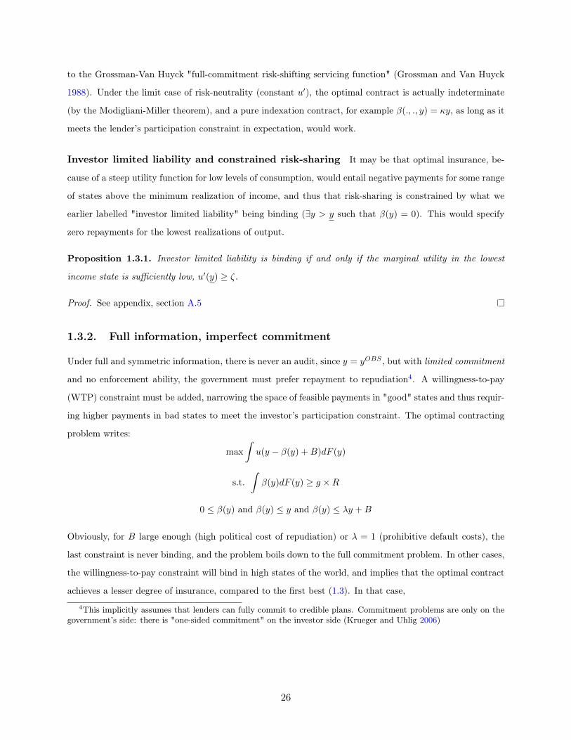
1.3.2. Full information, imperfect commitment

Under full and symmetric information, there is never an audit, since y = yOBS , but with limited commitment

and no enforcement ability, the government must prefer repayment to repudiation4. A willingness-to-pay

(WTP) constraint must be added, narrowing the space of feasible payments in "good" states and thus requir-

ing higher payments in bad states to meet the investor’s participation constraint. The optimal contracting

problem writes:

max

∫u(y − β(y) +B)dF (y)

s.t.∫β(y)dF (y) ≥ g ×R

0 ≤ β(y) and β(y) ≤ y and β(y) ≤ λy +B

Obviously, for B large enough (high political cost of repudiation) or λ = 1 (prohibitive default costs), the

last constraint is never binding, and the problem boils down to the full commitment problem. In other cases,

the willingness-to-pay constraint will bind in high states of the world, and implies that the optimal contract

achieves a lesser degree of insurance, compared to the first best (1.3). In that case,

4This implicitly assumes that lenders can fully commit to credible plans. Commitment problems are only on thegovernment’s side: there is "one-sided commitment" on the investor side (Krueger and Uhlig 2006)

26

• either the exogenous expenditure requirement can no longer be financed (autarky), which occurs if

∫ B1−λ

y

ydF (y) +

∫ y

B1−λ

λy +BdF (y) ≤ g ×R

• or, if λy + B is sufficiently large in expectation, the optimal contract calls for "maximum partial

indexation" above a threshold (where µ3 > 0), constant consumption (lower than in the first best)

in the intermediate range, and possibly binding limited liability constraint for low states. This is the

Kehoe and Levine 1993 problem for incentive-compatible contingent contracts.

Focusing on the feasible case, the first-order-conditions become:

f(y)(ζ − u′(y − β(y))) = µ3(y) + µ2(y)− µ1(y)

ζ(

∫β(y)dF (y)− gR) = 0 and µ1(y)β(y) = 0 and µ2(y)(y − β(y)) = 0 and µ3(y)(λy +B − β(y)) = 0

ζ, µ1(y), µ2(y), µ3(y) ≥ 0

with ζ, µ1, µ2, µ3 the Lagrangian "multipliers" (one scalar and three functions) corresponding, respectively,

to the investor participation, investor limited liability, borrower budget and borrower willingness to pay

constraints.

y

β(y

)

45 degrees lineFirst-best with no binding constraintFirst-best with binding non-negativityLimited commitment

Figure 1.3: Full information cases

27

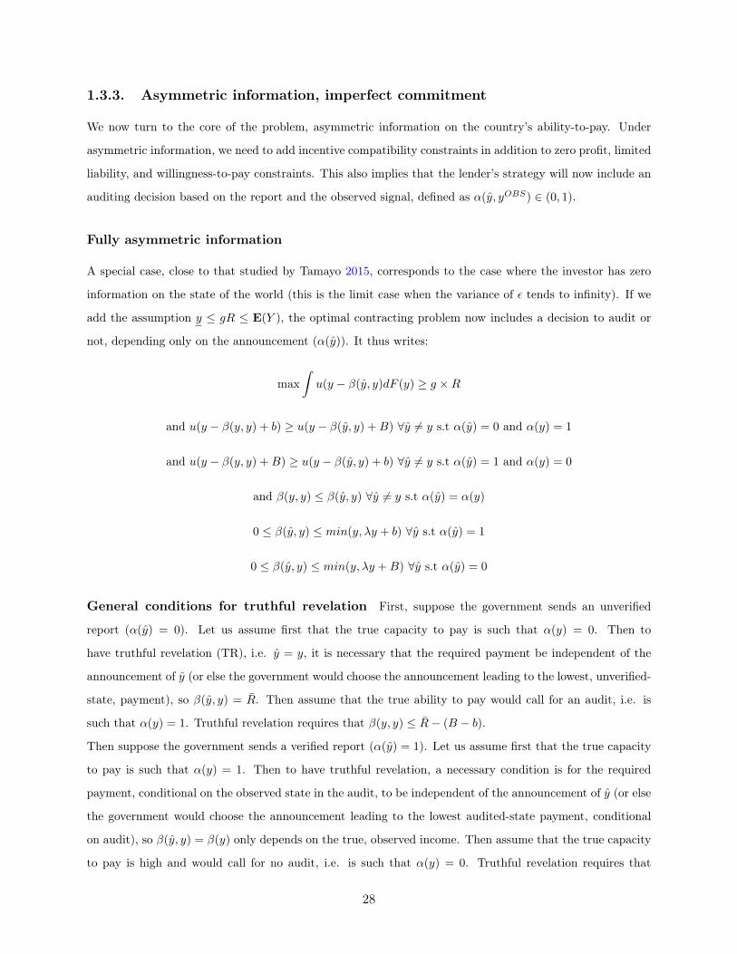
1.3.3. Asymmetric information, imperfect commitment

We now turn to the core of the problem, asymmetric information on the country’s ability-to-pay. Under

asymmetric information, we need to add incentive compatibility constraints in addition to zero profit, limited

liability, and willingness-to-pay constraints. This also implies that the lender’s strategy will now include an

auditing decision based on the report and the observed signal, defined as α(y, yOBS) ∈ (0, 1).

Fully asymmetric information

A special case, close to that studied by Tamayo 2015, corresponds to the case where the investor has zero

information on the state of the world (this is the limit case when the variance of ε tends to infinity). If we

add the assumption y ≤ gR ≤ E(Y ), the optimal contracting problem now includes a decision to audit or

not, depending only on the announcement (α(y)). It thus writes:

max

∫u(y − β(y, y)dF (y) ≥ g ×R

and u(y − β(y, y) + b) ≥ u(y − β(y, y) +B) ∀y 6= y s.t α(y) = 0 and α(y) = 1

and u(y − β(y, y) +B) ≥ u(y − β(y, y) + b) ∀y 6= y s.t α(y) = 1 and α(y) = 0

and β(y, y) ≤ β(y, y) ∀y 6= y s.t α(y) = α(y)

0 ≤ β(y, y) ≤ min(y, λy + b) ∀y s.t α(y) = 1

0 ≤ β(y, y) ≤ min(y, λy +B) ∀y s.t α(y) = 0

General conditions for truthful revelation First, suppose the government sends an unverified

report (α(y) = 0). Let us assume first that the true capacity to pay is such that α(y) = 0. Then to

have truthful revelation (TR), i.e. y = y, it is necessary that the required payment be independent of the

announcement of y (or else the government would choose the announcement leading to the lowest, unverified-

state, payment), so β(y, y) = R. Then assume that the true ability to pay would call for an audit, i.e. is

such that α(y) = 1. Truthful revelation requires that β(y, y) ≤ R− (B − b).

Then suppose the government sends a verified report (α(y) = 1). Let us assume first that the true capacity

to pay is such that α(y) = 1. Then to have truthful revelation, a necessary condition is for the required

payment, conditional on the observed state in the audit, to be independent of the announcement of y (or else

the government would choose the announcement leading to the lowest audited-state payment, conditional

on audit), so β(y, y) = β(y) only depends on the true, observed income. Then assume that the true capacity

to pay is high and would call for no audit, i.e. is such that α(y) = 0. Truthful revelation requires that

28

B − R ≥ b− β(y).

Repudiation-proof contracts A specific feature of an optimal sovereign debt contract (compared with

standard, enforceable debt) is that is must be "repudiation-proof" (see Bersem 2012). For the government to

prefer repayment to repudiation, we must have, in case the message leads to an audit, β(y, y) ≤ min(y, λy+b)

and in unaudited cases, β(y, y) ≤ min(y, λy + B). If the optimal contract C was not repudiation-proof,

we could construct an intermediary contract C ′ where in "non-repudiation states", repayments and audit

decisions are the same; and in repudiation states, audit decision is the same but the repayment obligation is

lowered to the cost of repudiation, so that it gives the government no incentive to repudiate. Such a contract

gives the same utility to the borrower, but strictly improves the creditor’s return (from 0 to min(y, λy+B) or

min(y, λy+b)) in former repudiation states. The dual implication is that this allows for another contract C ′′

with strictly lower repayments than C ′ in some range of states, to strictly improve the government’s expected

welfare, while still meeting the zero-profit condition. This is because repudiation, in this setup, is wasteful,

and does not extract additional value for the creditor. The "maximum recovery" strategy of exacting y is

not possible when there is repudiation risk. Recovery is determined by the government’s willingness-to-pay,

rather than by its ability-to-pay.

Constant repayments in unaudited states A classical result from the "costly state verification"

literature (e.g. Gale and Hellwig 1985, Townsend 1979) implies that in unaudited states, repayments should

be R, independent from the announcement. The proof is by contradiction: if there were two unaudited states

with unequal repayment obligations, the debtor would always report the state leading to a lower repayment

obligation. Let us define the audit region as A = {y|α(y) = 1} and the non-audit region as A. Then, for

y ∈ Aβ(y, y) = R.

Lower repayments in audited states Another result is that repayments must be lower in states

with an audit. The requirement here is even stronger: we must have, for y ∈ A, β(y, y) ≤ R − (B − b). By

contradiction, assume this is not the case (∃y ∈ A such that β(y, y) > R− (B− b)). Then announcing y ∈ A

yields u(y − R+B) > u(y − β(y, y) + b) and the incentive compatibility constraint is violated.

Proposition 1.3.2. A is a lower interval.

Proof. The constructive proof (slightly amending the proof of Lemma 3 in Tamayo 2015 by taking into

account that the cost of state verification is borne by the government rather than the investor) is given in

Appendix, section A.6.

29

The maximization problem can then be reduced to:

maxy∗,R,β(y)

∫ y∗

y

u(y − β(y) + b)dF (y) +

∫ y

y∗u(y − R+B)dF (y)

s.t.∫ y∗

y

β(y)dF (y) + R(1− F (y∗)) ≥ g ×R

0 ≤ β(y) ≤ min(y, λy + b) for y ∈ (y, y∗)

R ≤ min(y∗, λy∗ +B)

β(y) ≤ R− (B − b)

First-order conditions Focusing on the feasible case, the first-order-conditions require that there exists

ζ, µ1(y), µ2(y), µ3(y), µ4(y), µ5, µ6(y) the Lagrange "multipliers" (three scalar and four functions) such that:

f(y)(ζ − u′(y − β(y) + b)) = µ3(y) + µ2(y) + µ6(y)− µ1(y)

ζ(1− F (y))− (

∫ y

y∗u′(y − R+B) = µ4 + µ5 − µ6(y)

f(y)ζ(β(y∗)− R) + f(y)(u(y∗ − β(y∗) + b)− u(y∗ − R+B)) = −µ4 − λµ5

and µ1(y)β(y) = µ2(y)(y − β(y)) = µ3(y)(λy + b− β(y)) = µ6(y)(R− β(y)) = 0∀y ∈ A

and µ4(y∗ − R) = µ5(λy∗ +B − R) = 0

ζ, µ1(y), µ2(y), µ3(y), µ4, µ5, µ6(y) ≥ 0

We make the additional, reasonable assumptions y < b1−λ <

B1−λ < y. These conditions are necessary and

sufficient, given the concavity of the problem and the convexity of the constraint set. The shape of the

optimal contract in the fully asymmetric information case can then be derived from the first-order condi-

tions of the new maximization problem, close to the case studied Tamayo 2015. However, not all families

of contract defined by Tamayo can then be optimal, notably because here, the optimal incentive-compatible

contract must include a discontinuity in payments (of at least B − b) at the threshold between the auditing

and non-auditing region.

In the initial region (y, b1−λ ), only the ability to pay constraint can be binding, so µ3(y) = 0. Now, by a

simple slight amendment to lemma 1.3.1, investor limited liability will be binding (β(y) = 0) in the lowest

states as long as u′(y + b) < ζ. We define the liftoff point y1 as the point where u′(y1 + b) = ζ. Then, for

y ≥ y1, we have µ1(y) = µ2(y) = µ3(y) = µ6(y) = 0 and since ζ is independent from y, ζ−u′(y−β(y)+b) = 0

30

entails, when differentiating, by the implicit function theorem β′(y) = 1.

Therefore there is a region of states where the repayment schedule is given by β(y) = y − y1.

We then notice that, if the willingness to pay is binding at the auditing threshold in the audited states

(β(y∗) = λy∗ + b) the discontinuous jump in repayments at the auditing threshold y∗ must occur afterB

1−λ . Otherwise, the ability to pay constraint would be binding in the unaudited state at the threshold

(because y < λy +B), and the discontinuity would be insufficient to induce truthful revelation R− β(y∗) <

y∗ − β(y∗) = (1− λ)y∗ − b < B − b.

The schedule of repayments (0, then rising one for one with income) established above meets the willingness

to pay constraint in the audited states when β(y) = y − y1 = λy + b, a point we define as y2 = u′−1(ζ)−b+b1−λ .

Then a sufficient condition for the willigness to pay to be binding over a range of unaudited states is that

y2 <B

1−λ , i.e. ζ ≥ u′(B). If it is the case, the contract will have a region with β′(y) = λ in audited states. If

it is not the case, it may be that the optimal contract specifies an immediate jump from audit to non-audit

as soon as the willingness-to-pay constraint is binding in audited states.

Proposition 1.3.3. If the WTP constraint (with b) is binding for some unaudited states, the "unaudited"

willingness to pay (with B in the unaudited case) constraint will be binding at the threshold. Moreover, if

the willingness to pay is not binding at the unaudited threshold, the discontinuous jump in repayments must

be strictly larger than B − b, or the contract will be a simple two-step, fixed payments contract.

Proof. See Appendix, section A.7.

Whenever the optimal contract is not the two-step contract (0, B − b), and when the discontinuity is

indeed equal to B − b, we have R = λy∗ + B and the cutoff y∗ is thus uniquely determined by the lender’s

zero profit condition, given this schedule of optimal payments. Therefore, we can write, for the case with

binding willingness to pay, the binding zero profit participation constraint:

∫ u′−1(ζ)−b

y

0dF (y)+

∫ u′−1(ζ)1−λ

u′−1(ζ)−b(y−u′−1(ζ)+b)dF (y)+

∫ y∗

u′−1(ζ)1−λ

(λy+B)dF (y)+(1−F (y∗))(λy∗+B) = g×R

Features of the optimal contract First, risk-aversion of the borrower and risk-neutrality of the lender

implies (Townsend 1979) that consumption of the borrower should optimally be constant (i.e. β′(y) = 1)

across audited states whenever neither the non-negativity, nor the willingness to pay constraints bind. The

non-negativity constraint will bind in the lowest states if marginal utility in these states is sufficiently high

(e.g., for CRRA utility), by an argument similar to lemma 1.3.1.

Together with incentive compatibility constraints, the constant repayment in non-audited states implies that

repayments must be discontinuous at the auditing threshold y∗, since β(y∗) ≤ R− (B − b) ≤ λy∗ +B.

31

y

β(y

)45 degrees line

λy +Bλy + b

β(y)

Figure 1.4: Non-binding willingness to pay

y

β(y

)

45 degrees lineλy +Bλy + b

β(y)

Figure 1.5: Binding willingness to pay

The willingness-to-pay constraint may be binding over a region of intermediary states (1.5), or only be rele-

vant at the threshold of constant repayments (a "knife-edge case" pictured, for reference, in 1.4); and there

must be a discontinuous jump in repayments to ensure truthful revelation.

Therefore, generally, in the fully asymmetric information case, the optimal contract implies: (i) no state-

contingency in high states (constant repayments); (ii) zero payments in the lowest states for a general class

of utility functions exhibiting decreasing absolute risk aversion, since the investor limited liability constraint

binds when marginal utility of consumption in low states is high enough; and (iii) only partial insurance in

intermediate states, with a range of states where β′(y) = 1 (repayments rise one for one with income) in the

lowest states, and a range of states where β′(y) = λ in intermediary states.

Indexation is constrained at the bottom by limited liability; in intermediary states by limited commitment;

and at the top by asymmetric information.

Partial information

Let us turn to the general case with incomplete but not fully asymmetric information. Recall that creditors

(and the country) observe a publicly reported value of yOBS , an imperfect signal (yOBS = y + ε with ε ∼

N (0, σ2)). The optimal contracting problem now includes a decision to audit or not, depending on both the

32

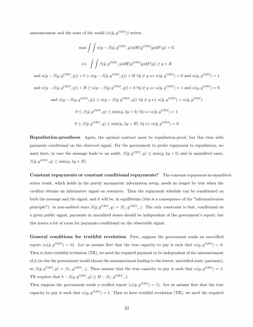
announcement and the state of the world (α(y, yOBS)) writes:

max

∫ ∫u(y − β(y, yOBS , y))dH(yOBS |y)dF (y) +G

s.t.∫ ∫

β(y, yOBS , y)dH(yOBS |y)dF (y) ≥ g ×R

and u(y − β(y, yOBS , y)) + b ≥ u(y − β(y, yOBS , y)) +B ∀y 6= y s.t α(y, yOBS) = 0 and α(y, yOBS) = 1

and u(y − β(y, yOBS , y)) +B ≥ u(y − β(y, yOBS , y)) + b ∀y 6= y s.t α(y, yOBS) = 1 and α(y, yOBS) = 0

and u(y − β(y, yOBS , y)) ≥ u(y − β(y, yOBS , y)) ∀y 6= y s.t α(y, yOBS) = α(y, yOBS)

0 ≤ β(y, yOBS , y) ≤ min(y, λy + b) ∀y s.t α(y, yOBS) = 1

0 ≤ β(y, yOBS , y) ≤ min(y, λy +B) ∀y s.t α(y, yOBS) = 0

Repudiation-proofness Again, the optimal contract must be repudiation-proof, but this time with

payments conditional on the observed signal. For the government to prefer repayment to repudiation, we

must have, in case the message leads to an audit, β(y, yOBS , y) ≤ min(y, λy + b) and in unaudited cases,

β(y, yOBS , y) ≤ min(y, λy +B).

Constant repayments or constant conditional repayments? The constant-repayment-in-unaudited-

states result, which holds in the purely asymmetric information setup, needs no longer be true when the

creditor obtains an informative signal on resources. Then the repayment schedule can be conditioned on

both the message and the signal, and it will be, in equilibrium (this is a consequence of the "informativeness

principle"): in non-audited stats β(y, yOBS , y) = β(., yOBS , .). The only constraint is that, conditional on

a given public signal, payments in unaudited states should be independent of the government’s report; but

this leaves a lot of room for payments conditional on the observable signal.

General conditions for truthful revelation First, suppose the government sends an unverified

report (α(y, yOBS) = 0). Let us assume first that the true capacity to pay is such that α(y, yOBS) = 0.

Then to have truthful revelation (TR), we need the required payment to be independent of the announcement

of y (or else the government would choose the announcement leading to the lowest, unverified-state, payment),

so β(y, yOBS , y) = β(., yOBS , .). Then assume that the true capacity to pay is such that α(y, yOBS) = 1:

TR requires that b− β(y, yOBS , y) ≥ B − β(., yOBS , .).

Then suppose the government sends a verified report (α(y, yOBS) = 1). Let us assume first that the true

capacity to pay is such that α(y, yOBS) = 1. Then to have truthful revelation (TR), we need the required

33

payment to be independent of the announcement of y (or else the government would choose the announcement

leading to the lowest, unverified-state, payment), so β(y, yOBS , y) = β(., yOBS , y). Then assume that the

true capacity to pay is such that α(y, yOBS) = 0: TR requires that B − β(y, yOBS , y) ≥ b− β(., yOBS , y).

1.4. The indexed debt contract

Indexing on the signal A key difference in our model from those of Bersem 2012 or Tamayo 2015 is

that lenders can condition both their monitoring strategy and the required payments on the observed, public

signal yOBS . The proposition below shows that repayments will be increasing in yOBS , conditional on the

absence of audit.

Proposition 1.4.1. In non-audited states, repayments are non-decreasing in yOBS = E(y|yOBS).

Proof. The proof is in appendix, section A.8

In other words, imperfect state-contingency occurs now at the top too, in expectation: the informative-

ness of the signal allows for partial insurance.

An example of an indexed debt contract Let us then define an "indexed debt contract" by the

following features:

• if α(y, yOBS) = 0, then β(y, yOBS , y) = β(., yOBS , .) = κ(yOBS) + B is constant in the announce-

ment and the true (unverified state), and only depends on public information yOBS , with κ′ ≥ 0; or

β(., yOBS , .) = 0 if marginal utility of consumption is high enough at yOBS

• if α(y, yOBS) = 1, then either β(y, yOBS , y) = β(., ., y) = β(y)−δ1y<yOBS is constant in the announce-

ment, and only depends on the true (verified) state of the world and on whether the true state is lower

than the signal; or β(y, yOBS , y) = β(., ., y) = 0 if marginal utility of consumption is high enough at

y.

• α(y, yOBS) = 1 if and only if y ≤ yOBS

Such a contract must respect the aforementioned conditions for truthful revelation. Neglecting the cases

with binding non-negativity, suppose y ≥ yOBS (the true capacity to pay is "high" relative to the signal).

If the government sends an unverified report, it has no incentive to lie: it is not audited, and gains utility

u(y − κyOBS − B + B), which does not depend on its announcement. If however the government sends a

message saying y ≤ yOBS , it is audited and gains: u(y−β(y) + b). Truthful revelation requires in particular:

u(y − β(yOBS) + b) ≤ u(y − κyOBS). Since β in audited states is either 1 or λ by the same arguments as in

the previous section, and since we must have κ ≤ λ to respect the willingness to pay constraint in high states,

34

this is always true if b is low enough, since y ≥ yOBS . A "high" capacity government will have incentives to

tell the truth in the indexed debt contract, since it avoids the cost of audit and pays less under indexation

than under observation.

Suppose on the contrary y < yOBS (the true capacity to pay is "low" relative to the signal). Will the

government have incentives to lie then? If the government sends a verified report, it has no incentive to

lie across the space of verified reports: it is audited, and gains utility u(y − β(y) + δ + b), which does not

depend on its announcement. If however the government sends a message saying y ≥ yOBS , it is unaudited

and gains: u(y−κyOBS). Truthful revelation requires: u(y−β(y) + δ+ b) ≥ u(y−κyOBS). Thus δ must be,

in particular, larger than the difference β(yOBS)− κyOBS − b (which can be negative if κ is close enough to

λ), so that even when ability to pay is close to the observed signal, a "low-capacity" government still does

not want to lie and mimic a "high-capacity" government. Thus incentive compatibility will, again, require

a discontinuity in repayments at the threshold of announcements requiring an audit, conditional on yOBS .

Note that the problem will never be for "higher than observed" capacity to pay, but rather for lower than

observed, given the cost of audit is borne by the borrower, and he might prefer "overpaying" rather than be

subjected to audit costs.

The contract must also meet the lender’s expected return constraint, meaning κ satisfies (with φ the CDF

of the standard normal distribution):

∫ y

y

∫ y

y

(β(y)− δ)dH(yOBS |y)dF (y) +

∫ y

y

∫ y

y

(κyOBS +B)dH(yOBS |y)dF (y) ≥ g ×R

∫ y

y

(

∫ y

y

(β(y)− δ)dφ(yOBS − y

σ) +

∫ y

y

(κyOBS +B)dφ(yOBS − y

σ))dF (y) ≥ g ×R

We have that κ ≤ λ to respect the willingness to pay constraint in all of the high states. We can show

that κ, for such a linear indexation scheme, is a decreasing function of the noise in the signal.

Proposition 1.4.2. κ, for such a linear indexation scheme, is a decreasing function of the variance of ε.

Proof. The proof is in appendix, section A.9

The repayment is increasing at a steeper slope when the signal is more informative.

1.4.1. Discussion

A number of features of the previous model may explain why state-contingency should be limited, but still

relevant. While borrower risk-aversion calls for increasing payments in the state of the economy, enforcement

and/or commitment problems prevent income from rising one for one with income in states where willingness

to pay is binding. Moreover, asymmetric information calls for incentive compatibility and thus limits the

35

state-contingency of payments in unobserved (high) states, while limited liability may bind in the lowest

range of states. It should also be noted that all these conditions are less likely to be met, when the risk-

free alternative rate is higher (the market could collapse altogether if the investor’s participation constraint

cannot be met). We thus obtain a ranking of optimal contracts depending on the nature of uncertainty:

• with full commitment, full information (symmetric), borrower risk-neutrality: the government fully

commits to repaying in the second period, depending on its income. Then the lender only lends if the

expectation of income is higher than the financing need, and the first-best is attained. Moreover, any

contract goes (by a variant of the Modigliani-Miller theorem).

• with full commitment, full information (symmetric), borrower risk-aversion: the government commits

to repay in the second period, depending on its income. But given risk-aversion, the optimum is

reached for constant consumption in period 2, i.e. full insurance.

• with repudiation risk, full information (symmetric), borrower risk-aversion: either there is partial

insurance and binding willingness to pay (if the expectation of willingness to pay is higher than

income), or zero financing can be achieved

• with full-commitment, but fully asymmetric information: we are in the classic “one-period” debt

model; the government commits to repaying the maximum of its income in case of an audit, so there

is constant repayment if no audit, audit if announcement below threshold, and maximum recovery of

assets if there is an audit.

• with repudiation risk, limited investor liability, and fully asymmetric information: repayments are

constant if there is no audit; there is an audit if the announced willingness to pay is below a threshold;

and repayments are either rising one for one with income, or constrained either by willingness to pay

or by investor limited liability if there is an audit.

• with repudiation risk and imperfect (but partially informative) signal, and risk-aversion: the payment

is an increasing function of the signal (because the signal itself informs on the true state of the world,

upon which the government prefers to have insurance), with constant repayments in unaudited states

(and audit conditional on both announcement and the signal). The repayment is increasing at a

steeper slope when the signal is more informative.

Indexed debt as imperfect hedging Comparative statics - that are beyond the scope of this thesis -

could study how risk-aversion parameters (using CRRA utility for example) interacts with σ and the lender

participation constraint in the design of the optimal contract: more risk aversion implies more demand for

insurance, but the feasibility of such insurance depends on the incentive compatibility constraint, which in

36

return depends on imperfect information. One could also assess the welfare loss from imperfect information

by having σ, the variance of ε, vary5. In the limit case where σ tends to infinity, we are back to the fully

asymmetric case of incentive-compatible sovereign debt, as in section 1.3.3.

When σ tends to 0, we are in the symmetric, full information case of section 1.3.2, corresponding to perfect

insurance constrained by the willingness to pay in the high states (see Obstfeld, Rogoff, and Wren-Lewis

1996, chapter 6).

For an information structure in between these polar cases, insurance will only be partial in the high states,

akin to an optimal "sovereign debt equity mix". The concept of such a partial insurance is that the signal

is used as an imperfect hedge, both reducing the width of the region requiring audits and increasing the

slope of indexation from 0 to a fraction of to the willingness to pay in the high-states region. If one thinks

of the true "income" of the borrower as unobservable, but of its growth rate as a verifiable and informative

signal, this provides a rationale for growth-rate indexation, and for examining partial, S-shaped indexation

formulas, to which we now turn in an asset pricing exercise.

5Note also that if we introduced an auditing cost for the lender as well (in the form, for example, of a waitingperiod to receive the proceeds), there could be a "Bayesian" auditing in mixed strategies, depending on the differencebetween yOBS and y

37

Chapter 2

Casino Royale: A Monte-Carlo

asset-pricing exercise

Our new Constitution is now established, and has an appearance that

promises permanency; but in this world nothing can be said to be certain,

except death and taxes.Benjamin Franklin, Letter to Jean-Baptiste Leroy, 1789

The previous chapter suggested that optimal indexation structures may take the form of S-shaped con-

tracts, with zero repayments at the bottom, and increasing repayments at the top with a slope constrained

by the quality of information on the borrower’s true ability to pay.

However, such a complex structure may give weight to an oft-repeated critique against sovereign debt in-

dexation, the difficulty to price GDP-linked instruments (see for example Griffith-Jones and Hertova 2013,

Blanchard, Mauro, and Acalin 2016). Market participants often argue that the volatility of their value and

the complexity of their payoff conditions are among the key impediments to a more widespread implemen-

tation of such bonds1.

GDP-indexed bonds relate payoffs to states of nature, which can, as a first approximation, be treated as

exogenous from the point of view of the investor. Monte-Carlo simulation methods drawing GDP from a

stochastic process, and expressing the valuation of the instrument as the average discounted value of payoffs

over simulations, should thus perform correctly. However, one cannot neglect the fact that GDP-indexed

bonds are risky instruments, and an appropriate stochastic discount factor should theoretically take into

account the correlation of the payoffs with investor’s consumption. They entail two different types of risk: a

binary default risk like plain-vanilla bonds, and a non-default volatility of payoffs due to the change in the un-1Reuters, "Investors say GDP bonds won’t work", Feb. 21, 2014

38

derlying value of GDP. These risks may affect the valuation of indexed bonds. It is not clear, however, what

additional difficulties are associated with pricing GDP-indexed debt compared to any other state-contingent

security.

Finally, a specific feature of GDP-indexed bonds may explain the difficulty to price them. The underlying

process for GDP is itself likely to be uncertain and volatile, especially in emerging economies where out-

put can be thought of having a stochastic trend (M. Aguiar and Gopinath 2007). In that case, indexation

formulas that include a barrier on the level of GDP as well as on its growth rate may generate additional

volatility in the expected net present value of future payments, with each shock to trend affecting the whole

stream of future payoffs.

In this chapter, we want to simply show, in a theoretically agnostic way, how these types of parameters

affect the pricing of GDP-indexed bonds, and thus constrain the amount of financing that the sovereign

can obtain through such risk-sharing agreements. As an example, we can conjecture that more risk-averse

lenders imply lower prices for any amount of indexed debt (at a given amount of non-contingent debt); and

that the interaction of level barriers and persistence in the GDP process can create a lot of volatility in the

payoffs, thus reducing the value of indexed debt. The price of a GDP-indexed bond crucially depends on:

1. the indexation formula that has been chosen

2. the underlying statistical process that drives output

3. the risky discount factor that is used to price the instrument

We start by reviewing past attempts at pricing GDP-indexed instruments, before turning to each of

these three categories of parameters in more detail.

2.1. Past attempts at pricing GDP-indexed instruments

Several methods have been employed in the past to provide a practical framework for GDP-linked securities

pricing. A number of them simply use risk-free pricing and a given statistical process for GDP, yielding

a price function by taking the average of the net present value of the bond over Monte Carlo simulations.

Other researchers have explicitly modelled default risk in structural terms, although they usually preserve

the assumption of risk-neutral investors for tractability.

• Discrete-time models have the advantage of being easily comparable to plain-vanilla bond pricing,

and to actually match the payoff structure of existing GDP-instruments, whose coupons are released

at regular intervals depending on annual GDP growth. A discrete-time framework, where default

thresholds - expressed in terms of debt-to-GDP ratios - are inferred from observed prices of plain-

vanilla bonds and assumption of lender risk-neutrality, was developed by Mauro and M. Chamon

39

2006, who then use it to show the reduction in default risk (and in borrowing costs) resulting from

issuing indexed debt.

• An alternative discrete time model is that of Myiajima 2006, who also uses a risk-neutral pricing

kernel, discounting expected payoffs at the risk-free (inflation-adjusted) rate, but explicitly models

the sovereign’s tax revenues but neglects default risk. Since it is more concerned with the possibility

that the sovereign may "overpay" than with default, it quantifies additional tax receipts due to excess

growth in each period, in order to derive a limit on the issuance of GDP-indexed instruments.

• Continuous time models, besides being mathematically more elegant, avail themselves of widely

adopted asset pricing results, notably the Black-Scholes option valuation formula (treating GDP-

indexed instruments, loosely speaking, as call options on GDP growth above a threshold). Schinkus’s

assumption of a simple geometric Brownian motion for GDP, with caps and floors on coupon payments

(Schinckus 2013) is an example of such a model, although it assumes zero default risk and a risk-free

discounting of payoffs.

• Kruse et al.’s model, which also features a standard geometric Brownian motion for GDP and zero

default risk (Kruse, Meitner, and Schröder 2005), expands the reflection by taking into account vari-

ous indexation formulas, notably time-varying principal in addition to time-varying coupons, and by

showing that most indexation formulas can be treated as call options on the GDP index, valued with

the Black-Scholes formula.

• The most complete model of GDP-indexed debt pricing is provided in a recent paper by Ruban,

Vitiello, and Poon 2014, who distinguish between potential GDP (which follows a geometric standard

Brownian motion) and actual GDP (with the output gap following an Ornstein-Uhlenbeck mean-

reverting process). The country is assumed to default on all of its outstanding debt when the value of

the bond exceeds a share of potential GDP (rather than actual GDP) calibrated to match empirical

default probabilities. Ruban et al. also take into account the volatility of payoffs by using a risk-averse

pricing kernel (in the reduced form of the Esscher transform), rather than simply taking the mean

NPV of future payoffs.

Our asset pricing methodology includes elements from several of these models, but attempts to explic-

itly quantify the relative importance of default-risk reduction and risk-aversion, while at the same time

parametrizing the model for various indexations formulas and GDP processes. To give an idea of what the

securities look like in the real world, I plot in figure 2.1 the market prices of three GDP-indexed securities

issued during sovereign debt restructurings (Ukraine, Greece, and Argentina), retrieved from the Bloomberg

platform as of May 2016.

40

(a) Greek GDP warrant (b) Ukrainian GDP warrant

(c) Argentinian GDP warrant

Figure 2.1: The prices of three GDP warrants issued during restructurings

2.2. The role of the indexation formula

2.2.1. Existing designs for GDP-indexed debt

Several potential designs for real-indexed debt, growth-indexed bonds, or GDP-indexed bonds have been

experimented in the past. We review some of them below:

• Bosnia and Herzegovina’s GDP-linked warrant : The GDP-linked warrants pay a coupon if (a) GDP

hits a predetermined target level and remains at such a level for two years and (b) GDP per capita

rises above US$2,800 in 1997 units, adjusted for German consumer price inflation.

• Bulgaria’s Additional Interest Payment : Bulgaria’s GDP-linked security was part of the Brady debt

restructuring. They entailed an additional interest payment (AIP) of 12 of annual growth on exchanged

bonds, payable upon two conditions: that the GDP level (its nature - nominal or real - and reference

index was not specified...) exceeded 125% of its 1993 level; and that GDP grew year-on-year. It also

included a call option, i.e. the right for Bulgaria to buy back the AIP at par whenever it wanted,

41

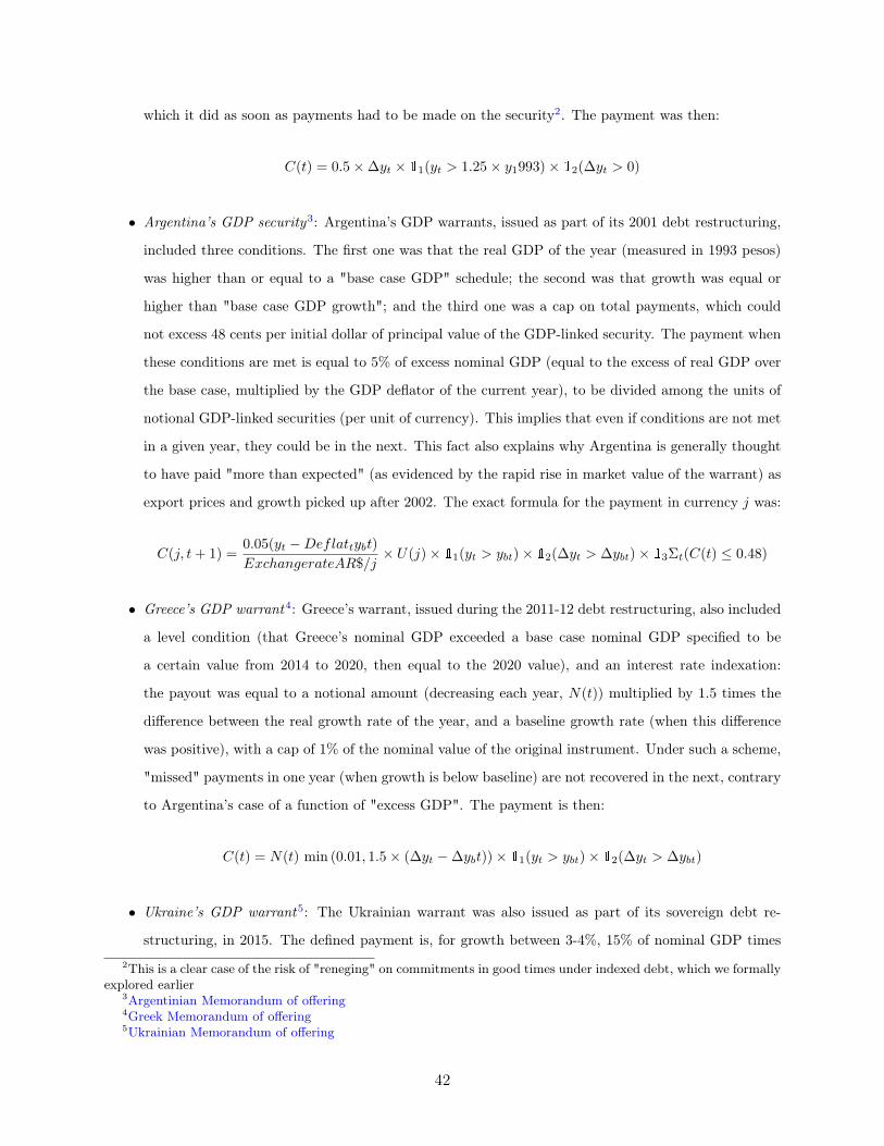
which it did as soon as payments had to be made on the security2. The payment was then:

C(t) = 0.5×∆yt × 11(yt > 1.25× y1993)× 12(∆yt > 0)

• Argentina’s GDP security3: Argentina’s GDP warrants, issued as part of its 2001 debt restructuring,

included three conditions. The first one was that the real GDP of the year (measured in 1993 pesos)

was higher than or equal to a "base case GDP" schedule; the second was that growth was equal or

higher than "base case GDP growth"; and the third one was a cap on total payments, which could

not excess 48 cents per initial dollar of principal value of the GDP-linked security. The payment when

these conditions are met is equal to 5% of excess nominal GDP (equal to the excess of real GDP over

the base case, multiplied by the GDP deflator of the current year), to be divided among the units of

notional GDP-linked securities (per unit of currency). This implies that even if conditions are not met

in a given year, they could be in the next. This fact also explains why Argentina is generally thought

to have paid "more than expected" (as evidenced by the rapid rise in market value of the warrant) as

export prices and growth picked up after 2002. The exact formula for the payment in currency j was:

C(j, t+ 1) =0.05(yt −Deflattybt)ExchangerateAR$/j

× U(j)× 11(yt > ybt)× 12(∆yt > ∆ybt)× 13Σt(C(t) ≤ 0.48)

• Greece’s GDP warrant4: Greece’s warrant, issued during the 2011-12 debt restructuring, also included

a level condition (that Greece’s nominal GDP exceeded a base case nominal GDP specified to be

a certain value from 2014 to 2020, then equal to the 2020 value), and an interest rate indexation:

the payout was equal to a notional amount (decreasing each year, N(t)) multiplied by 1.5 times the

difference between the real growth rate of the year, and a baseline growth rate (when this difference

was positive), with a cap of 1% of the nominal value of the original instrument. Under such a scheme,

"missed" payments in one year (when growth is below baseline) are not recovered in the next, contrary

to Argentina’s case of a function of "excess GDP". The payment is then:

C(t) = N(t) min (0.01, 1.5× (∆yt −∆ybt))× 11(yt > ybt)× 12(∆yt > ∆ybt)

• Ukraine’s GDP warrant5: The Ukrainian warrant was also issued as part of its sovereign debt re-

structuring, in 2015. The defined payment is, for growth between 3-4%, 15% of nominal GDP times

2This is a clear case of the risk of "reneging" on commitments in good times under indexed debt, which we formallyexplored earlier

3Argentinian Memorandum of offering4Greek Memorandum of offering5Ukrainian Memorandum of offering

42

the real GDP growth exceeding 3%; for growth faster than 4%, 40% of nominal GDP times the real

GDP growth beyond 4%, in addition to the full amount for the range of 3 to 4% growth. There will

be no payments until GDP reaches $125.4 billion, compared with GDP of about $80bn-$84bn in 2015

(although at a particularly depressed exchange rate), and payments will be capped at 1% of GDP

from 2021 to 2025. The payment is then a function of GDP:

P (t) = 11(yt > 125.4)12(∆yt > 0.03)× yt min[0.01; 0.15× (min(0.04,∆yt)− 0.03)

+13(∆yt > 0.04)× 0.4× (∆yt − 0.04)]

2.2.2. Classification of indexation formulas

We suggest that GDP-linked securities can therefore fall under several broad classes (or combinations

thereof):

• "pure" sovereign equity, which pays a share of the sovereign equivalent of "profits", whether GDP (trills

as in Athanasoulis, Shiller, and Wincoop 1999), government spending (as proposed by Barro 1995 in

his study of optimal debt management), or proceeds of a sovereign wealth fund. The redemption value

of such "shares" depends on the level of a real or nominal variable, most often GDP, and not on its

recent growth rate.

• bonds with a coupon rate depending on current GDP growth: in this case, the coupon rate is an

increasing function of the growth rate - in general linear. In the simplest case, it is equal to annual

GDP growth (allowing for potential data revisions); or an affine function of that growth rate, of the

form r = c + α × g - and sometimes more specifically r = c + α(g − g∗) with g∗ a baseline or trend

expected growth rate.

• cap and floors on interest rates Many historical cases (and theoretical justifications related to our first

chapter on limited risk sharing) include a lower bound (most often equal to 0) on the interest rate,

and sometimes an upper bound capping the coupon at a ceiling rate (this can be thought of as a case

when the observed high "signal" is not truly indicative of the sovereign’s ability to pay).

• bonds combining an interest rate indexed to GDP growth and a condition on the level of GDP : such

bonds have been proposed (and, as we saw earlier, experimented) to avoid very high payments during

years when a country catches up with output trend after a deep crisis, but remains in low absolute

standing and thus has a limited capacity to pay. However, they imply more volatile payoffs, possibly

very high in the best cases, and thus may prove costly to issue as part of a "normal time" financing

strategy, especially if lenders are risk averse.

43

• bonds with automatic maturity extension: such bonds, similar to the "contingent-convertible" securities

that have become a standard of bank capital regulatory requirements (Brooke et al. 2013, or Levy-

Yeyati6), would see their maturity automatically lengthened in case of adverse shocks, to avoid liquidity

(rollover) crises.

All of these broad models entail trade-offs for borrowers and lenders alike, depending on:

• the data-generating process for output: one can conjecture that the more persistent the output

level, the more the inclusion of a level condition increases the volatility of payoffs (although it is also

likely to improve the ability to pay of the country, thus reducing default risk). For a (close to) unit-

root output process, output may fail to recover its previous trend even in the medium run, and thus a

condition on the trend, while it reduces expected payments for the holder, improves insurance against

catastrophic events for the issuer.

• the insurance/cost trade-off for the borrower (or risk-return trade-off from the point of view

of the investor): including floors and caps in the indexation formula for interest rates (of the form

r = min(max(r, c+ α × (g − g∗)), r)) reduces the variance of payments, and thus the required return

for investors, but it also reduces the insurance properties of contingent debt for the issuer. A floor of

0, for example, is consistent with a version of investor limited liability where there can be no loss in

principal on debt-like instruments outside default events.

• the commitment/moral hazard trade-off : a "perfect" indexation formula would insulate the

issuer against any types of variation in income, but it would at the same time lower incentives to

pursue growth-oriented policies (or not to pursue growth-destructive policies), or at the very least

generate incentives to misreport data. Similarly, call options or ceilings reduce upside risk in terms of

payments from the point of view of the issuer, but they limit the amount of "profit-sharing" and thus

the value of the instrument, making it closer to the "fully asymmetric" case of chapter 1.

2.3. The role of output statistical properties

2.3.1. The risk of model mis-specification

The uncertainty over future GDP is one of the main reasons why GDP-indexed bonds have been deemed

difficult to price. Indeed, if the GDP process was purely deterministic, or even if its stochastic process was

perfectly known, simulations-based methods would be sufficient to price expected future paths for payoffs of

indexed debt. The limitation to fair pricing is thus related to model mis-specification, rather than to GDP

6Peterson Institute Real Time Economic Issues Watch, February 2015

44

volatility itself. This is what has been labelled "uncertainty premia" in some of the literature (Presno and

Pouzo 2012).

Establishing the "true" stochastic process followed by output is both beyond the scope of this thesis, and

generally thought by "humble macroeconomists" (John H Cochrane 1991) to be close to impossible: with

finite data, any unit root process, for example, is essentially indistinguishable from a stationary process with

roots close enough to 1. Unit root tests can be easily "fooled" by processes with sufficiently long periodicity.

In the wise words of Christiano and Eichenbaum 1990, "we don’t know" and thus "we don’t care".

The investor in indexed debt, however, "cares" very much about the forecastability of GDP over the dura-

tion of the bond, since it will determine the expected return. The issuing sovereign is also interested in the

expected repayment and its volatility over the lifetime of the security, which crucially depends on whether

the GDP process can be accurately forecast at the time of issuance.

A first approach consists of estimating historical processes for GDP under various assumptions (i.i.d shocks

on growth, deterministic trend plus growth shocks, stochastic trends plus persistent growth shocks...) and

choosing the one that best fits the data (according to either the Box-Jenkins methodology for stationary pro-

cesses, or some information criterion). Another is to assume the simplest model (i.i.d. normally distributed

shocks on growth) and determine whether the loss due to model mis-specification is likely to be large or not.

The importance of the stochastic output process, however, can vary significantly depending on the nature

of the indexation formula. Indeed, if the formula only includes contemporary growth, or even excess growth

over baseline, in the payment of contemporary coupons, model mis-specification is not likely to be a serious

concern; at worse, investors may overestimate or underestimate the average growth rate, but, as shown by

Mauro and M. Chamon 2006, this is unlikely to have a material effect on the securities’ net present value. If,

however, the indexation formula includes a level condition, then a "mistaken" estimate of the GDP process

can result in large variations in the valuation of the security, since it affects the entire trajectory of future

payments.

2.3.2. Persistence and volatility

A number of processes for GDP can be envisaged. They broadly fall into three main classifications:

• i.i.d. shocks: growth is normally distributed, so that the level of GDP is log-normal, and growth is

unpredictable from one period to another.

• persistent shocks: trend growth is deterministic, but shocks to output each period are persistent and

propagate in future periods

• stochastic trend : trend growth itself is both stochastic and persistent, so that shocks to trend propagate

into permanent effects on the level of GDP and persistent effects on the growth rate

45

The main parameters of the GDP stochastic process affecting the value of the instrument are, naturally, the

expected value of growth, its persistence, and its volatility. All else equal, a higher expected value of growth

increases the value of the instrument, by increasing payoffs which are positively dependent on growth.

A higher volatility, however, can have both negative and positive effects on the price of the instrument.

First, all else equal, a risk-averse investor will dislike volatility, all the more so when its own consumption

path is highly correlated with the GDP process. Then, depending on whether expected growth is above or

below the trigger growth threshold (in formulas including baseline growth), volatility can have negative or

positive effects on the price: if it is above, more volatility increases the risk of falling below the threshold

and thus decreases the value of the instrument, while if expected growth is below the trigger value, more

volatility increases the likelihood of payment and thus the value of the instrument (see Marcos Chamon,

Costa, and Ricci 2008). Finally, more volatility implies more skewness of the GDP in levels, and thus, for

indexation formulas based on the value of GDP, a positive effect, as higher growth rates are associated with

higher values of GDP in level.

Persistence of the output process can affect the value of the instrument in several ways. First, it implies

that lower payments in a given year are associated with lower payments in later years, so that it increases,

ex ante, the variability of the instrument’s net present value over its lifetime. The second consequence of

persistence in the output process is that, when a condition on GDP levels is included in the payoff structure,

the probability of payment is itself very persistent (which is not the case if shocks are purely transitory and

output remains around the stable, baseline trend).

2.4. The role of investor risk-aversion

2.4.1. The world is not enough: growth correlations

Risk-neutral pricing implies that indexed debt is almost a "free lunch" under perfect observability and no

moral hazard: it reduces default risk and thus borrowing costs, and smooths the distribution of payoffs for

investors. It is, however, of limited use to understand why investors balk at financing state-contingent debt.

In this section, we thus assume that foreign investors are not able to fully diversify the income risk that

is part of the GDP-linked instrument’s payoff volatility. This is the case, for example, if growth rates are

positively correlated across countries, so that an investor’s consumption is high in times where payoffs on

the GDP-linked bond are high: following J. Cochrane 2001, this implies that GDP-linked bonds have payoffs

that are negatively correlated with the marginal utility of consumption, and thus that they should trade at

a lower price than instruments with a similar expected return but less correlation with consumption growth.

Despite large volatility in growth rates across countries and time, currently available financial instruments

46

indeed do not provide a simple way to diversify macroeconomic risk by “hedging” against a country’s or a

region’s growth prospects (Athanasoulis, Shiller, and Wincoop 1999; Williamson 2005): (a) stock market

indexes, especially in emerging economies, are often too narrow and far from representative of economy-wide

performance; (b) by definition, sovereign debt does not provide an upside if a country’s performance is better

than expected, and can only share risk very bluntly through outright restructuring in the reverse case; and (c)

proxies (such as raw materials prices for commodity exporters) do not perfectly match a country’s economic

success or disarray, and may be endogenously affected by a country’s performance if it is large enough.

2.4.2. A toy model of risk-averse investors

Under risk-averse pricing, a trade-off arises, between the lower price commanded by indexed debt (due to

its volatility) and its hedging virtues for the borrower. Assume a two-period case. In the first period, the

government finances expenditure g with debt, which can take two forms: indexed debt akin to Shiller 1993’s

trills (S), each unit of which pays a share κ of period-2 output, and traditional non-contingent bonded debt

(B) which pays one unit of output. κ is normalized so that expected payment (in the absence of default) is

E(κY2) = 1.

The government’s financing constraint in period 1 is thus given by: pBB+ pSS = g where pB and ps denote

the prices of bonded debt and indexed debt, respectively. Prices are taken as given by the government but

are to be determined in equilibrium by demand from foreign investors. In period 2, output is stochastic,

and the government can choose to default or to repay its debt. Its budget constraint, conditional on default

decision (δ = 1 denoting default), is thus given by:

C2(δ,B, S) = Y2(1− λδ)− (1− δ)(B + SκY2)

and the government defaults if and only if C2(1, B, S) > C2(0, B, S). For any given amount of non-contingent

debt B, if the country defaults at income Y ∗, then it defaults for any income below Y ∗ as long as S ≤ λκ .

Foreign investors have initial wealth W0, and can invest it in three types of available securities: a risk-free

international storage technology with a gross return of 1, the economy’s bonds, and the economy’s GDP

shares. They also receive exogenous stochastic income YW , which we assume to be correlated with Y2 by

Y2 = YW +ε. Denoting by δ the Boolean variable associated with the country’s decision to default, investors’

wealth next period, conditional on repayment decision, is given by

W1(δ) = YW + (1− δ)(B + κSY2) + (W0 − pBB − pSS)

47

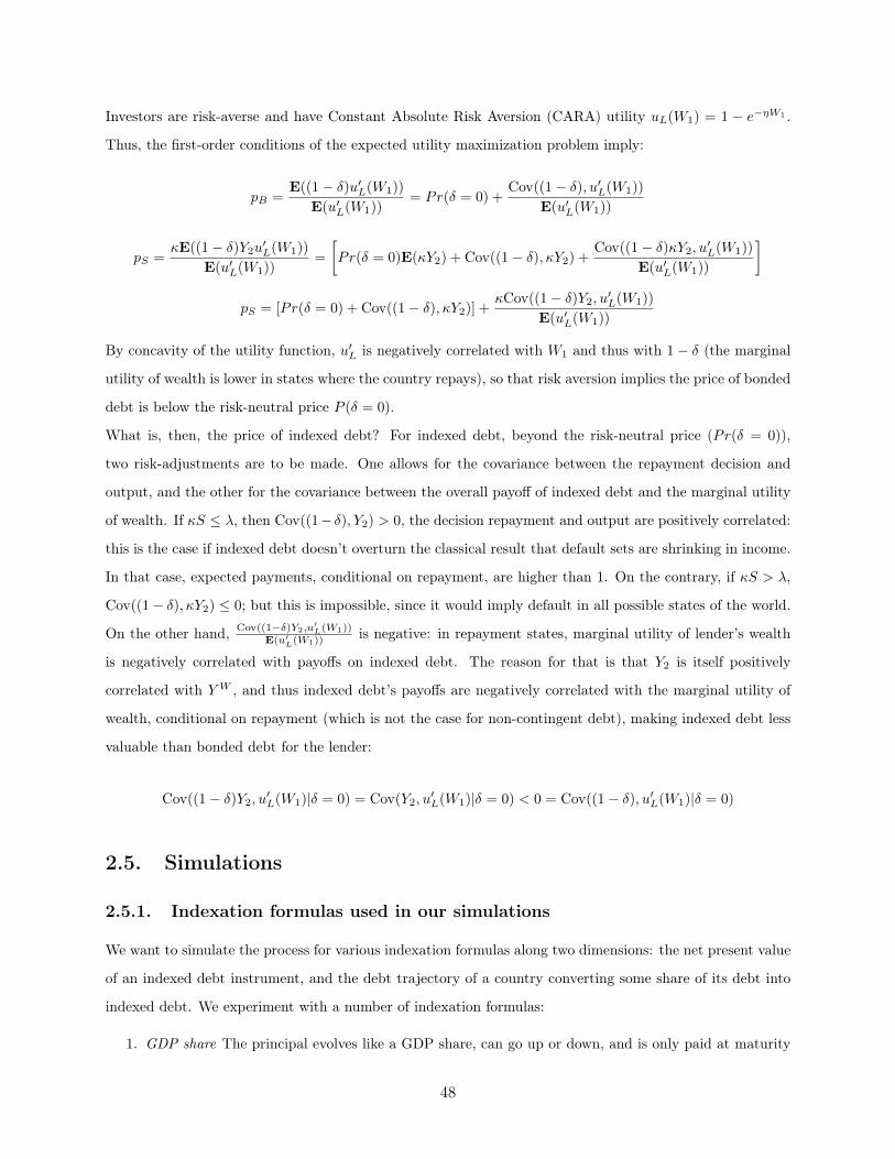
Investors are risk-averse and have Constant Absolute Risk Aversion (CARA) utility uL(W1) = 1 − e−ηW1 .

Thus, the first-order conditions of the expected utility maximization problem imply:

pB =E((1− δ)u′L(W1))

E(u′L(W1))= Pr(δ = 0) +

Cov((1− δ), u′L(W1))

E(u′L(W1))

pS =κE((1− δ)Y2u

′L(W1))

E(u′L(W1))=

[Pr(δ = 0)E(κY2) + Cov((1− δ), κY2) +

Cov((1− δ)κY2, u′L(W1))

E(u′L(W1))

]

pS = [Pr(δ = 0) + Cov((1− δ), κY2)] +κCov((1− δ)Y2, u

′L(W1))

E(u′L(W1))

By concavity of the utility function, u′L is negatively correlated with W1 and thus with 1− δ (the marginal

utility of wealth is lower in states where the country repays), so that risk aversion implies the price of bonded

debt is below the risk-neutral price P (δ = 0).

What is, then, the price of indexed debt? For indexed debt, beyond the risk-neutral price (Pr(δ = 0)),

two risk-adjustments are to be made. One allows for the covariance between the repayment decision and

output, and the other for the covariance between the overall payoff of indexed debt and the marginal utility

of wealth. If κS ≤ λ, then Cov((1− δ), Y2) > 0, the decision repayment and output are positively correlated:

this is the case if indexed debt doesn’t overturn the classical result that default sets are shrinking in income.

In that case, expected payments, conditional on repayment, are higher than 1. On the contrary, if κS > λ,

Cov((1− δ), κY2) ≤ 0; but this is impossible, since it would imply default in all possible states of the world.

On the other hand, Cov((1−δ)Y2,u′L(W1))

E(u′L(W1)) is negative: in repayment states, marginal utility of lender’s wealth

is negatively correlated with payoffs on indexed debt. The reason for that is that Y2 is itself positively

correlated with YW , and thus indexed debt’s payoffs are negatively correlated with the marginal utility of

wealth, conditional on repayment (which is not the case for non-contingent debt), making indexed debt less

valuable than bonded debt for the lender:

Cov((1− δ)Y2, u′L(W1)|δ = 0) = Cov(Y2, u

′L(W1)|δ = 0) < 0 = Cov((1− δ), u′L(W1)|δ = 0)

2.5. Simulations

2.5.1. Indexation formulas used in our simulations

We want to simulate the process for various indexation formulas along two dimensions: the net present value

of an indexed debt instrument, and the debt trajectory of a country converting some share of its debt into

indexed debt. We experiment with a number of indexation formulas:

1. GDP share The principal evolves like a GDP share, can go up or down, and is only paid at maturity

48

(zero-coupon). This model (S1) is the simplest, where we assume the one-period implicit return to

be a multiple of the one-period growth rate of GDP (approximated by the first-difference of the log),

r = α∆(yt) (notice that it includes the possibility of capital losses during years of negative growth).

2. growth rate coupon, wih floor and cap The coupon is equal to a linear function of the growth rate,

with a floor at 0% and a cap at 15%. Coupons are paid every year, but the principal remains fixed

and repaid at maturity. The second formula (S2) thus includes a floor and a cap on payments:

r = min(r + max(0, α∆(yt)), r).

3. excess growth over baseline coupon The coupon is the baseline interest rate plus excess growth over

base case growth, with floor at 0% and cap at 15%. Coupons are paid every year, but the principal

remains fixed. The third formula S3 is thus based on excess growth over the historical trend before

time t0, r = min(r + max(0, α∆(yt)− g), r).

4. excess growth over baseline coupon, with level condition The coupon is the baseline interest rate plus

excess growth over baseline, with floor at 0% and cap at 10%. There is a level condition: the baseline

coupon is paid every year; the reduction in coupons occurs whenever growth is below the threshold;

but a strictly positive indexed part of the coupon is paid only if GDP exceeds trend. The principal

remains fixed and is always paid at maturity. The fourth formula S4 is therefore similar to the third,

but positive indexed payments are only made in years where GDP is above a pre-determined trend in

level (yt ≥ yt0 + (t− t0)g).

5. GDP share and level condition The principal evolves like a GDP share, can go up or down, is only

paid at maturity (no coupons), but pays out only if GDP exceeds trend in level at maturity. The fifth

formula S5 is therefore similar to the very first one, but it includes a similar condition on GDP levels

as the fourth.

2.5.2. Output process used in the simulations

To assess how several forms of indexed debt fare when confronted to various possible data-generating process

for output, we envisage three possible stochastic processes for real GDP (denoting output as Yt and its log

as yt).

The first one simply assumes that growth rates are i.i.d and normally distributed around their historical

mean, so that log output can be thought of as the sum of a deterministic trend with drift equal to mean

growth, and a white noise shock: yt = a+ g × t+ ε1,t.

The second one is a trend stationary, persistent, process, with a transitory shock following an AR(1) com-

ponent, and a deterministic trend, so that we have yt = a+ g × t+ zt where zt = ρ1zt−1 + ε1,t.

49

Finally, the third process, inspired from M. Aguiar and Gopinath 2006, encompasses the other two. It states

that GDP (in levels) follows Yt = Γtezt . This includes two components, loosely labelled as a trend and

a cycle. The cyclical component zt is modelled as an AR(1) process (zt = ρzzt−1 + εzt), so that shocks

to z eventually die out, while the trend Γt is modelled as the cumulative product of trend growth shocks

(Γt = egtΓt−1) with gt = (1 − ρg)µg + ρggt−1 + εg,t, so that any shock to g has a permanent effect on the

level of output and a persistent effect on the growth rate.

2.5.3. Pricing kernel used in the simulations

We use a form of the Esscher transform pricing method, as in Gerber and Shiu 1994. This section draws

heavily on Ruban, Vitiello, and Poon 2014. Taking an economy with one risky asset with flows xt at time

t and a risk-free bond yielding r, let F0,t denote the time 0 forward price of this cashflow xt, for t ∈ (0, T ],

where T is the bond’s term to maturity.

An investor who owns a unit of the stream of risky cashflows bases his decisions on a risk-averse exponential

utility function u(xt) = 1−e−ηxt . We assume that there exists a derivative security that provides a payment

of πt at time t > 0, where πt is some function of the cashflows xt. Let V0,t denote the time 0 forward price

for the derivative security. The number of derivative contracts z that the investor would want to buy or sell

can be derived by maximising the expected utility function W (z) = E(u(xt + z(πt − V0,t)). Using the first

order condition, we can write: 0 = E(u′(xt + z(πt − V0,t)))(πt − V0,t).

If we now impose z = 0, implying that the derivative is fairly priced and therefore the representative investor

would not want to buy or sell any derivative contracts in this equilibrium, we obtain V0,t = E(πtu′(xt))

E(u′(xt)), which

must hold for any derivative security, including the case where πt = xt (the security itself), in which case

F0,t = V0,t.

Therefore the (forward) asset specific pricing kernel is given by m(xt) = e−ηxt

Et(e−ηxt )and the forward value of

the cashflow can be written in standard form as F0,t = Et(xte−ηxt

E(e−ηxt )).

Assuming the simulation is run for N stochastic paths for debt and output, at each point t ∈ (0, T ] there are

N states of the world, each with an equal probability of occurring pti = 1N .

Then we have, using our Monte Carlo simulations:

F0,t =

N∑i=1

ptixtim(xti) =

N∑i=1

1

Nxti

Ne−ηxti∑Ni=1 e

−ηxti) =

N∑i=1

xtie−ηxti∑N

i=1 e−ηxti

50

Assuming a constant risk free interest rate rF , the spot price of the bond can then be written as the discounted

sum of these cashflow streams:

P0 =

T∑t=1

e−rF tF0,t =

T∑t=1

e−rF tN∑i=1

xtie−ηxti∑N

i=1 e−ηxti

One possible intuition behind this risk aversion is that the country should be able to diversify away its

own risk "for free" (in actuarially fair terms), but not the aggregate market risk. The variance of payoffs

itself does not generate discounting relative to the risk-free case; rather, the correlation between investors’

consumption and GDP outcomes is what drives the risk premium. Thus our single risk aversion parameter η

can be thought of as a shortcut for a more explicit modelling of consumption growth for the world investor,

and GDP growth in the country, valuing the resulting payoffs with a given utility function, e.g. CRRA

with parameter γ. Suppose output is yi = yW + xi for country i, with xi orthogonal to the process for

world income. Suppose further that the respective variances of the shocks are σw and σx. This generates

ν = corr(yi, yW ) = σw

σx. We could then study the sensitivity of the price of indexed debt to the parameter

ν. Then our model can be thought of as one which concatenates both ν and γ into a unique risk aversion

parameter, η.

2.5.4. Methodology and results

We proceed in several steps. First, for each of the possible output processes, we calibrate the slope parameter

of each indexation formulas in order for them to have an expected, risk-neutral NPV equal to that of the

plain-vanilla bond, in the absence of default. In terms of our earlier model, this amounts to the normalization

that κ is calibrated so that expected payment (without default) is E(κY2) = 1.

Then, we proceed to implement the risk-neutral pricing method, to gauge the risk-neutral value of the reduc-

tion in default risk afforded by indexed debt, under various shares of indexed debt. In terms of the earlier

model, the idea is to disentangle the positive impact of price resulting from Cov((1− δ), Y2) > 0.

The next step is to implement a risk-averse pricing method, by making the investor’s stochastic discount

factor correlated with payoffs. In terms of our model, the idea is to value the negative price effect resulting

from Cov((1− δ)κ(Y2), u′L(W1)) < Cov((1− δ), u′L(W1)). We experiment with two steps. The first consists

in shutting down default risk, thus gauging the negative price effect which is specific to indexed debt and

arises from: Cov(κ(Y2), u′L(W1)|δ = 0) < 0 = Cov((1− δ), u′L(W1)|δ = 0) Finally, we do sensitivity analyses

to: the risk aversion parameter; the share of indexed debt; and the "model mis-specification" risk.

Our methodology therefore actually consists of a mixture of the Mauro and M. Chamon 2006 (debt ratios as

default triggers, discrete time) and the Ruban, Vitiello, and Poon 2014 (investor risk-aversion) approaches,

while performing comparative statics on the output process and the nature of the indexation formula. We

51

then run a Monte Carlo simulation of the flows, discounted with the relevant stochastic discount factor, in

order to value the indexed security (with a limit case of risk-neutral investors corresponding to a CARA

parameter of zero for the investor’s utility function). Matlab codes for the simulations are available at the

following address.

Calibrating the model We first calibrate the standard deviation of shocks to output (both transitory

and trend shocks), as well as primary balance shocks to reasonable values, close to those used in Mauro and

M. Chamon 2006. We then modify the parameters of the various indexation formulas so that, in expectation,

they all yield a default-risk-free return equal to the plain vanilla bond over the period.

Doing so requires imposing, in the risk-neutral case, that the expected payment (in the absence of default

risk) on GDP-indexed securities equals the (deterministic) net present value of plain vanilla bonds, with

κ(Yt, δYt) the general indexation formula, c the coupon rate on plain vanilla bonds, and T the maturity of

the bond:

E0

(T∑t=1

κ(Yt, δYt)

(1 + r)t

)= 1

For the "pure growth rate" case, the only degree of liberty is the slope of indexation. For other formulas,

we could in theory follow two paths, either by letting the floors and caps vary while keeping the slope at its

previously calibrated value, or by varying the slope. For purposes of simplicity and comparability, we let the

slope of indexation αi vary and choose reasonable parameters for floors (0%) and caps (15%).

The αi to be calibrated for each formula Si correspond to the following:

• S1: xT =∏Tt=1(1 + α1gt)

• S2: xt = min(max(rmin, α2gt), rmax)

• S3: xt = c+ min(max(rmin − c, α3(gt − g)), rmax − c)

• S4: xt = (c+ min(max(rmin − c, (gt − g)1gt<g + α4(gt − g))1gt>g1∏tk=1(1+gk)>(1+g)t , rmax − c))

• S5: xT =∏Tt=1(1 + α5gt)1∏T

t=1(1+gk)>(1+g)T

The slopes we find are reproduced in table 2.1: The simulated distributions of net present values for

Table 2.1: Calibrated slopes on growth or excess growth in indexation formulas

Process Formula 1 Formula 2 Formula 3 Formula 4 Formula 5i.i.d. shocks 2.2481 2.1823 0.9995 1.2662 4.1057Persistent shocks 2.3201 2.1359 0.9981 1.3405 4.8093Stochastic trend 1.8448 2.1450 1.0087 1.0475 2.4939

indexed debt are given, for process 1, in figure 2.2. Other simulations for process 2 and 3 are reproduced in

52

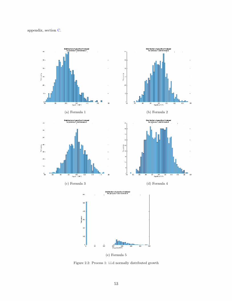
appendix, section C.

(a) Formula 1 (b) Formula 2

(c) Formula 3 (d) Formula 4

(e) Formula 5

Figure 2.2: Process 1: i.i.d normally distributed growth

53

One can immediately observe that the distribution of payoffs in NPV is less volatile for formulas 1 to 3

than for formulas 4 and 5. Including a level condition on GDP relative to baseline makes payoffs much more

volatile (conditional on a given NPV), since it implies paying a high amount in the states where repayment

occurs to compensate for the large number of states with zero payoffs. The fact that slopes are very close

for processes 1 and 2 for the first four formulas is also an indication that model mis-specification is unlikely

to be a major concern in that case.

Moreover, the nature of the output process affects the volatility of payoffs in NPV: the more persistent are

shocks to output, the more volatile are payoffs in NPV for a given mean value. This effect is particularly

visible for formulas 2 and 3 (because the floors and caps are more often binding when output is more

persistent), and for formulas 4 and 5, again, because the level condition is more frequently binding under

more persistent output processes, thus requiring a higher slope of indexation.

Risk neutral pricing with default shocks We seek to understand the limits of risk-neutral pricing

methodologies for GDP-indexed bonds. To that end, we first replicate the Mauro and M. Chamon 2006

pricing methodology, updating parameters, and applying it to various indexation formulas, and various data

generating processes for output and the primary balance.

We start from a debt accumulation equation. We abstract from exchange rate dynamics, and simply assume

that debt-to-GDP ratios (DtYt ) accumulate as the combined result of a GDP process (Yt) and a primary

balance process (PBt, expressed as percentage of current period GDP).

Dt

Yt=

Dt−1(1 + it)

Yt−1(1 + gt)(1 + π)− PBt

A specific assumption in our model is that, while growth is taken to be exogenous, the primary balance is

partly endogenous: it evolves as the weighted average of a normally distributed random shock around its

historical mean, and a reaction to GDP growth (positive when growth is above its unconditional expectation,

and negative when growth is below), so that deficits are contra-cyclical (the primary balance is procyclical).

If we include a share θ of indexed debt, we now have:

Dt

Yt=Dt−1

Yt−1

θ(1 + iINDt ) + (1− θ)(1 + it)

(1 + gt)− PBt

The next core assumption, specific to this section is that risk-neutral investors price bonds fairly, so

that plain-vanilla bonds are valued at a spread over risk-free US Treasury bonds perfectly compensating for

their additional default risk, in present value terms. From the observed spread on emerging market bonds,

one can therefore infer a default probability such that, when discounted at the risk-free rate, payoffs on the

54

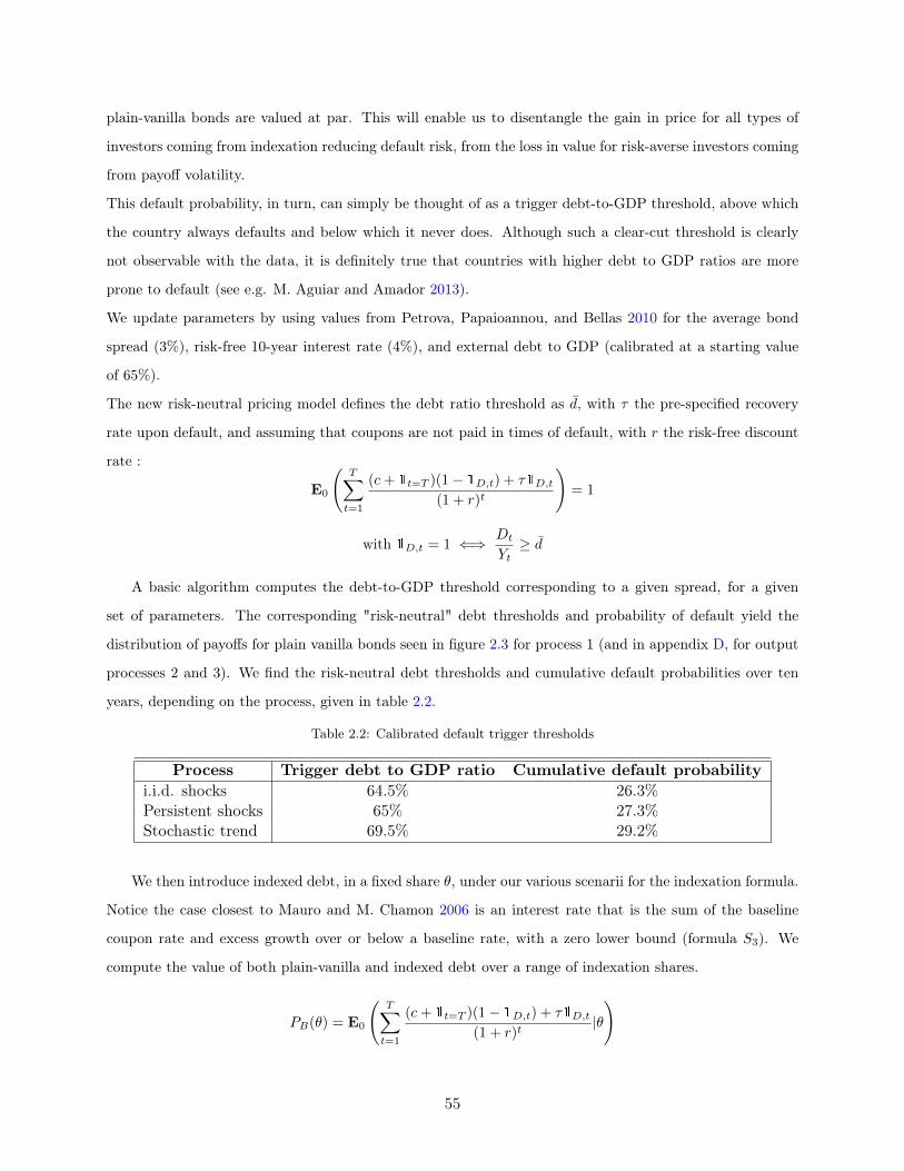
plain-vanilla bonds are valued at par. This will enable us to disentangle the gain in price for all types of

investors coming from indexation reducing default risk, from the loss in value for risk-averse investors coming

from payoff volatility.

This default probability, in turn, can simply be thought of as a trigger debt-to-GDP threshold, above which

the country always defaults and below which it never does. Although such a clear-cut threshold is clearly

not observable with the data, it is definitely true that countries with higher debt to GDP ratios are more

prone to default (see e.g. M. Aguiar and Amador 2013).

We update parameters by using values from Petrova, Papaioannou, and Bellas 2010 for the average bond

spread (3%), risk-free 10-year interest rate (4%), and external debt to GDP (calibrated at a starting value

of 65%).

The new risk-neutral pricing model defines the debt ratio threshold as d, with τ the pre-specified recovery

rate upon default, and assuming that coupons are not paid in times of default, with r the risk-free discount

rate :

E0

(T∑t=1

(c+ 1t=T )(1− 1D,t) + τ1D,t(1 + r)t

)= 1

with 1D,t = 1 ⇐⇒ Dt

Yt≥ d

A basic algorithm computes the debt-to-GDP threshold corresponding to a given spread, for a given

set of parameters. The corresponding "risk-neutral" debt thresholds and probability of default yield the

distribution of payoffs for plain vanilla bonds seen in figure 2.3 for process 1 (and in appendix D, for output

processes 2 and 3). We find the risk-neutral debt thresholds and cumulative default probabilities over ten

years, depending on the process, given in table 2.2.

Table 2.2: Calibrated default trigger thresholds

Process Trigger debt to GDP ratio Cumulative default probabilityi.i.d. shocks 64.5% 26.3%Persistent shocks 65% 27.3%Stochastic trend 69.5% 29.2%

We then introduce indexed debt, in a fixed share θ, under our various scenarii for the indexation formula.

Notice the case closest to Mauro and M. Chamon 2006 is an interest rate that is the sum of the baseline

coupon rate and excess growth over or below a baseline rate, with a zero lower bound (formula S3). We

compute the value of both plain-vanilla and indexed debt over a range of indexation shares.

PB(θ) = E0

(T∑t=1

(c+ 1t=T )(1− 1D,t) + τ1D,t(1 + r)t

|θ

)

55

Figure 2.3: Calibration of default cases to match par value of plain vanilla bond: Process 1

PS(θ) = E0

(T∑t=1

(κ(Yt, δYt))(1− 1D,t) + τ1D,t(1 + r)t

|θ

)

with 1D,t = 1 ⇐⇒ Dt

Yt≥ d and θ =

StBt + St

The resulting distribution of payoffs in NPV for a share of indexed debt of 50% is shown in figure 2.4 for

process 1 (similar results for processes 2 and 3 are shown in appendix E). Tables 2.3, 2.4, 2.5, respectively

measure, for the cases with 50%, 20% and 80% indexed debt, the cumulative 10-year default probability.

The main takeaway here is that increasing the share of indexed debt tends to reduce default risk, especially

for formulas 2 to 4, although this effect may be reversed for larger shares of indexed debt. However, it tends

to increase default risk for the last formula, as it implies a rarely occurring, but large burden of debt in the

last period, which is almost certain to trigger default when payments are indeed made.

Moreover, indexed debt is all the more valuable in terms of default risk reduction when the output process

is very persistent, whether through persistent transitory shocks or through stochastic trend shocks, since it

stabilizes the debt trajectory within "safe" boundaries.

Table 2.3: Cumulative default probability, 50% indexed debt, risk-neutral lenders

Process Formula 1 Formula 2 Formula 3 Formula 4 Formula 5i.i.d. shocks 23.2% 24.4% 26.6% 4.7% 67.1%Persistent shocks% 22.4% 19.8% 23.0% 4.0% 82.4%Stochastic trend 3.6% 11.8% 16.1% 7.1% 10.9%

56

(a) Formula 1 (b) Formula 2

(c) Formula 3 (d) Formula 4

(e) Formula 5

Figure 2.4: Process 1: i.i.d normally distributed growth

Introducing risk-aversion We then introduce risk-averse pricing, in two steps. We first shut down

the default option, in order to measure the reduction in value arising from payoff volatility for indexed debt

57

Table 2.4: Cumulative default probability, 20% indexed debt, risk-neutral lenders

Process Formula 1 Formula 2 Formula 3 Formula 4 Formula 5i.i.d. shocks 25.8% 26.0% 24.7% 13.3% 38.1%Persistent shocks 23.6% 21.1% 21.5% 11.6% 43.4%Stochastic trend 17.5% 21.3% 22.4% 16.6% 15.7%

Table 2.5: Cumulative default probability, 80% indexed debt, risk-neutral lenders

Process Formula 1 Formula 2 Formula 3 Formula 4 Formula 5i.i.d. shocks 25.0% 23.4% 22.2% 1.2% 83.8%Persistent shocks 22.1% 20.4% 21.0% 1.2% 94.5%Stochastic trend 6.0% 10.5% 10.0% 2.6% 27.4%

relative to bonded debt, for a given, identical expected repayment in net present value over the life of the

bond.

The most affected formula, naturally, is formula 5, which has the highest variance in terms of final payoffs (it

can pay zero in roughly half of the cases, when the level condition at the end of the period is not met; thus,

for a given NPV of 100, it pays a lot in half of the cases, creating large volatility in payoffs and commanding

a very low risk-adjusted price). We plot below the risk-adjusted values of each formula for each process, with

no default risk and thus a simple adjustment for volatility (see table 2.6).

Table 2.6: Volatility-adjusted NPV of indexed debt without default risk

Process Formula 1 Formula 2 Formula 3 Formula 4 Formula 5i.i.d. shocks 97.3313 86.5350 86.9973 86.8795 23.3633Persistent shocks 99.0496 86.4795 86.8465 86.6863 20.4030Stochastic trend 77.9760 86.3105 86.7502 86.5816 22.7974

We then allow for default to occur in equilibrium. This implies that non-contingent debt is now also

risky, due to the built-in contingency of defaults (exactly "how" risky it is now depends on the recovery rate

specified). Therefore, we cannot use the same debt-to-GDP trigger thresholds as before, because they were

calibrated on the basis of a simple risk-neutral equivalent par price between emerging and risk-free debt. We

recalibrate the default trigger thresholds to take into account the reduction in value arising from default risk

premia, identifying default triggers debt-to-GDP ratios which are consistent with a (risk-averse) pricing at

par of plain vanilla bonds, for a parameter value of η = 0.005 as in Ruban, Vitiello, and Poon 2014.

We find the following risk-averse debt thresholds and cumulative default probabilities over ten years, de-

pending on the process, when matching the risk-adjusted value of the non-contingent bonds to par (see table

2.7).

Using these newly (higher) calibrated debt thresholds and (lower) cumulative default probabilities, we

can now recompute the risk-adjusted value of indexed debt payoff, using our ad hoc pricing method, and

58

Table 2.7: Calibrated default trigger thresholds, with risk aversion

Process Trigger debt to GDP ratio Cumulative default probabilityi.i.d. shocks 69.5% 10.6%Persistent shocks 68.5% 11.4%Stochastic trend 79.5% 11.9%

perform comparative statics on the share of indexation, as before. The simulated results for process 1 is

shown in figure 2.5 (processes 2 and 3 are shown in Appendix G). The cumulative default probabilities for

a 50% share of indexed debt are given in table 2.8.

Table 2.8: Cumulative default probability, 50% indexed debt, risk-averse lenders

Process Formula 1 Formula 2 Formula 3 Formula 4 Formula 5i.i.d. shocks 7.1% 6.7% 6.7% 5.5% 50.2%Persistent shocks 8.4% 10.6% 7.9% 3.8% 75.8%Stochastic trend 0.1% 3.0% 4.1% 8.4% 1.1%

Overall, this chapter enabled us to perform comparative statics on various types of S-shaped indexation

formulas, while noticing the importance of the stochastic nature of the output process for the valuation of

GDP-indexed bonds. Indexed debt may be particularly valuable when the output process is more persistent,

thus justifying GDP level conditions; but when we introduce investor risk-aversion as an additional constraint

limiting sovereign risk-sharing, we notice that this implies an additional trade-off in terms of borrowing costs.

To understand exactly how this constraint affects a structural model of default risk, we turn, in the next

section, to a general equilibrium model of sovereign default with two types of debt and risk-averse investors.

59

(a) Formula 1 (b) Formula 2

(c) Formula 3 (d) Formula 4

(e) Formula 5

Figure 2.5: Process 1: i.i.d normally distributed growth

60

Chapter 3

You only live twice: Recursive general

equilibrium models of indexed debt

The burden of the national debt consists not in its being so many millions, or

so many hundred millions, but in the quantity of taxes collected every year to

pay the interest. If this quantity continues the same, the burden of the

national debt is the same to all intents and purposes, be the capital more or

less.Thomas Paine, The Rights of Man, part. II

Our partial equilibrium approach in the previous sections yielded several useful insights. Indexation is

unlikely to be perfect, due to imperfect observability, commitment problems and limited investor liability.

Moreover, lender risk aversion can partly explain why state-contingent debt is less ubiquitous than would

seem optimal at first glance. In order to exploit these insights in a consistent framework, we turn to general

equilibrium models of indexed debt.

Macroeconomic models of defaultable sovereign debt have a fruitful history, starting with Eaton and Gersovitz

1981, with quantitative implications further explored by M. Aguiar and Gopinath 2006, Arellano 2008, Alfaro

and Kanczuk 2005, among others. Some papers have also tried to adapt the traditional Eaton-Gersovitz

recursive equilibrium framework to the case of output-indexed debt. In particular, Faria 2007 and Sandleris,

Saprizza, and Taddei 2011 have attempted an analysis of the case where all debt is indexed, taking the form

of indexation as given, while Durdu 2009 performed comparative statics on the slope of indexation.

We intend to enrich existing models of indexed debt by allowing for both types of bonds to be issued in

equilibrium, since the previous sections point to the intuition that it is indeed optimal for the government to

have an "equity-debt" mix rather than purely non-contingent, or purely indexed liabilities. To do so, lender

61

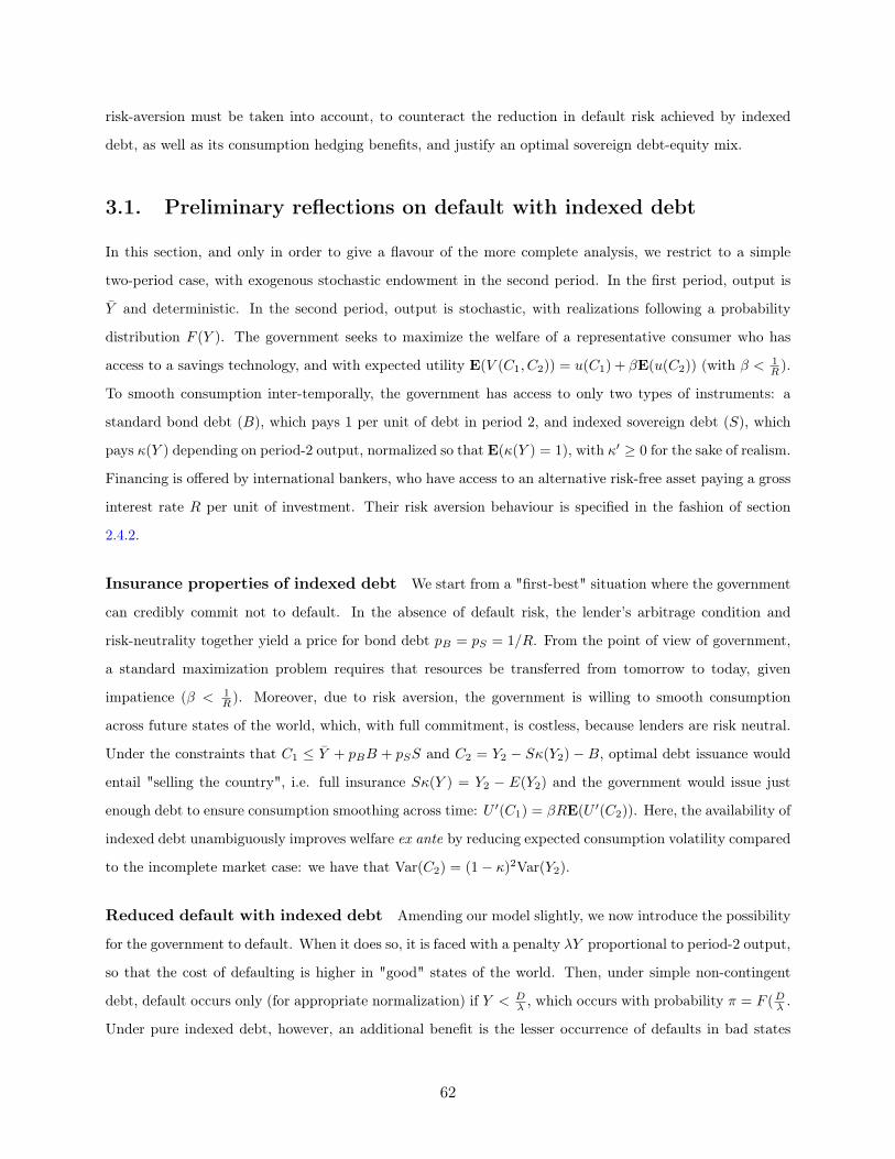
risk-aversion must be taken into account, to counteract the reduction in default risk achieved by indexed

debt, as well as its consumption hedging benefits, and justify an optimal sovereign debt-equity mix.

3.1. Preliminary reflections on default with indexed debt

In this section, and only in order to give a flavour of the more complete analysis, we restrict to a simple

two-period case, with exogenous stochastic endowment in the second period. In the first period, output is

Y and deterministic. In the second period, output is stochastic, with realizations following a probability

distribution F (Y ). The government seeks to maximize the welfare of a representative consumer who has

access to a savings technology, and with expected utility E(V (C1, C2)) = u(C1) + βE(u(C2)) (with β < 1R ).

To smooth consumption inter-temporally, the government has access to only two types of instruments: a

standard bond debt (B), which pays 1 per unit of debt in period 2, and indexed sovereign debt (S), which

pays κ(Y ) depending on period-2 output, normalized so that E(κ(Y ) = 1), with κ′ ≥ 0 for the sake of realism.

Financing is offered by international bankers, who have access to an alternative risk-free asset paying a gross

interest rate R per unit of investment. Their risk aversion behaviour is specified in the fashion of section

2.4.2.

Insurance properties of indexed debt We start from a "first-best" situation where the government

can credibly commit not to default. In the absence of default risk, the lender’s arbitrage condition and

risk-neutrality together yield a price for bond debt pB = pS = 1/R. From the point of view of government,

a standard maximization problem requires that resources be transferred from tomorrow to today, given

impatience (β < 1R ). Moreover, due to risk aversion, the government is willing to smooth consumption

across future states of the world, which, with full commitment, is costless, because lenders are risk neutral.

Under the constraints that C1 ≤ Y + pBB + pSS and C2 = Y2 − Sκ(Y2)− B, optimal debt issuance would

entail "selling the country", i.e. full insurance Sκ(Y ) = Y2 − E(Y2) and the government would issue just

enough debt to ensure consumption smoothing across time: U ′(C1) = βRE(U ′(C2)). Here, the availability of

indexed debt unambiguously improves welfare ex ante by reducing expected consumption volatility compared

to the incomplete market case: we have that Var(C2) = (1− κ)2Var(Y2).

Reduced default with indexed debt Amending our model slightly, we now introduce the possibility

for the government to default. When it does so, it is faced with a penalty λY proportional to period-2 output,

so that the cost of defaulting is higher in "good" states of the world. Then, under simple non-contingent

debt, default occurs only (for appropriate normalization) if Y < Dλ , which occurs with probability π = F (Dλ .

Under pure indexed debt, however, an additional benefit is the lesser occurrence of defaults in bad states

62

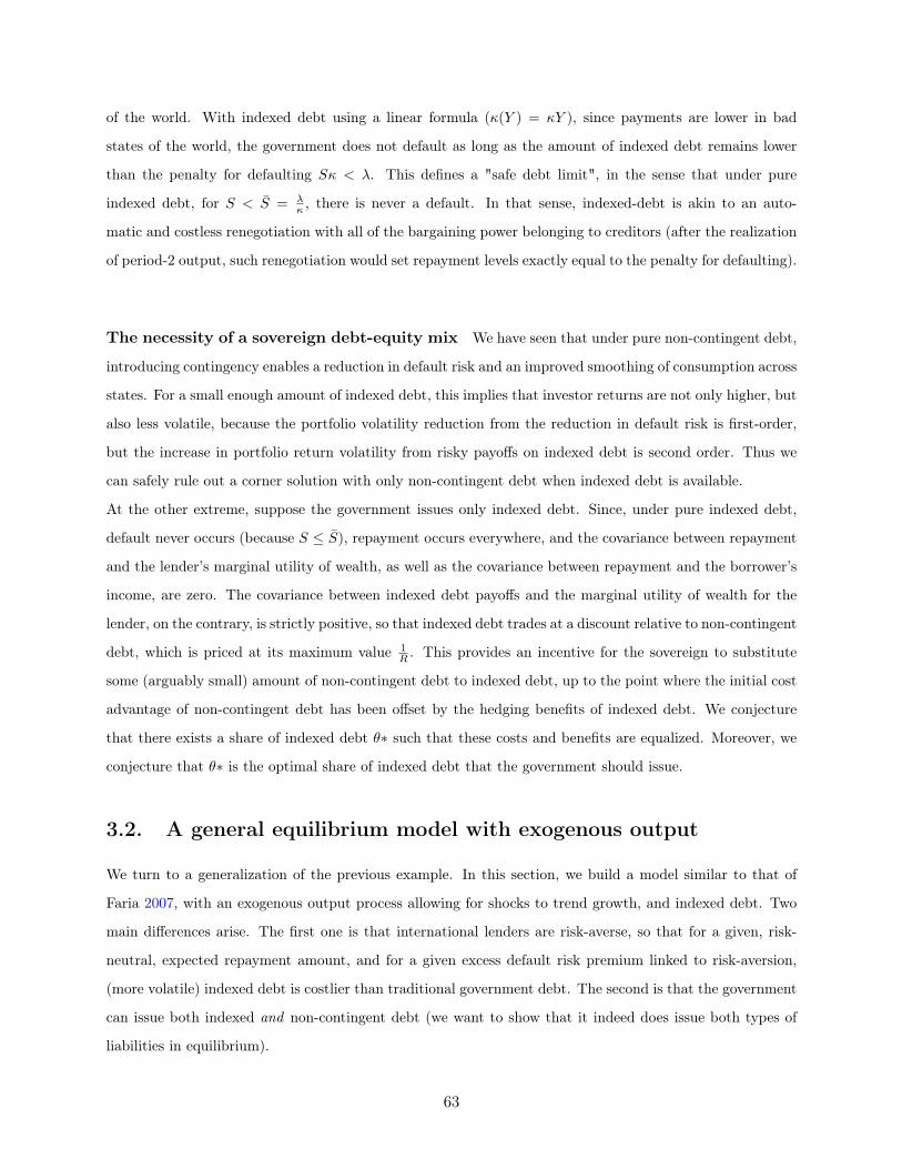
of the world. With indexed debt using a linear formula (κ(Y ) = κY ), since payments are lower in bad

states of the world, the government does not default as long as the amount of indexed debt remains lower

than the penalty for defaulting Sκ < λ. This defines a "safe debt limit", in the sense that under pure

indexed debt, for S < S = λκ , there is never a default. In that sense, indexed-debt is akin to an auto-

matic and costless renegotiation with all of the bargaining power belonging to creditors (after the realization

of period-2 output, such renegotiation would set repayment levels exactly equal to the penalty for defaulting).

The necessity of a sovereign debt-equity mix We have seen that under pure non-contingent debt,

introducing contingency enables a reduction in default risk and an improved smoothing of consumption across

states. For a small enough amount of indexed debt, this implies that investor returns are not only higher, but

also less volatile, because the portfolio volatility reduction from the reduction in default risk is first-order,

but the increase in portfolio return volatility from risky payoffs on indexed debt is second order. Thus we

can safely rule out a corner solution with only non-contingent debt when indexed debt is available.

At the other extreme, suppose the government issues only indexed debt. Since, under pure indexed debt,

default never occurs (because S ≤ S), repayment occurs everywhere, and the covariance between repayment

and the lender’s marginal utility of wealth, as well as the covariance between repayment and the borrower’s

income, are zero. The covariance between indexed debt payoffs and the marginal utility of wealth for the

lender, on the contrary, is strictly positive, so that indexed debt trades at a discount relative to non-contingent

debt, which is priced at its maximum value 1R . This provides an incentive for the sovereign to substitute

some (arguably small) amount of non-contingent debt to indexed debt, up to the point where the initial cost

advantage of non-contingent debt has been offset by the hedging benefits of indexed debt. We conjecture

that there exists a share of indexed debt θ∗ such that these costs and benefits are equalized. Moreover, we

conjecture that θ∗ is the optimal share of indexed debt that the government should issue.

3.2. A general equilibrium model with exogenous output

We turn to a generalization of the previous example. In this section, we build a model similar to that of

Faria 2007, with an exogenous output process allowing for shocks to trend growth, and indexed debt. Two

main differences arise. The first one is that international lenders are risk-averse, so that for a given, risk-

neutral, expected repayment amount, and for a given excess default risk premium linked to risk-aversion,

(more volatile) indexed debt is costlier than traditional government debt. The second is that the government

can issue both indexed and non-contingent debt (we want to show that it indeed does issue both types of

liabilities in equilibrium).

63

3.2.1. The environment

Output The output process, inspired from M. Aguiar and Gopinath 2006, states, as process 3 in our

Monte Carlo simulations of 3, that Yt = Γtezt . This includes two components, a "trend" and a "cycle"

(we follow the literature in labelling the transitory component as the "cycle" despite the absence of defined

periodicity). The cyclical component zt is modelled as an AR(1) process (zt = ρzzt−1 +εzt), so that shocks to

z eventually die out, while the trend Γt is modelled as the cumulative product of growth shocks (Γt = gtΓt−1)

with log(gt) = (1− ρg)(log(µg)− c) + ρg log(gt−1) + εg,t, so that any shock εg,t to g has a permanent effect

on the level of output and a persistent effect on the growth rate.

I outline in Appendix B some issues related to potential future work on endogenizing output dynamics in

such a general equilibrium model of indexed and non-contingent debt.

Households The government maximizes the representative household’s intertemporal utility, which has

the following form: E0[Σ+∞0 βtU(Ct)] with U(Ct) = (Ct)

1−σ

1−σ . Households are unable to borrow on interna-

tional markets, so that the government smooths consumption on their behalf.

Asset structure The government can issue two types of assets. It can borrow either through non-

contingent B-debt (bt), promising to pay one unit of output next period, or through indexed S-debt (st),

contingent on realizations of output, each unit of which promises to pay κ(Yt) next period. The indexation

formula is normalized so that in the absence of default or risk aversion, both kinds of debt have the same

expected payoff, E(κ(Yt)) = 1.

Budget constraint Default is assumed to have proportional output costs λYt. Let δt denote the Boolean

variable associated with the decision to default in period t (so that δt = 0 means repayment). Since defaulting

also means loosing access to capital markets, the economy’s budget constraint is given by:

Ct = Yt(1− δtλ) + (1− δt)qB(st+1, bt+1, Yt)bt+1 + (1− δt)qS(st+1, bt+1, Yt)st+1 − (1− δt)bt − (1− δt)stκ(Yt)

where qB(st+1, bt+1, Yt) and qS(st+1, bt+1, Yt) denote respectively the price of non-contingent and contingent

debt due next period. To prevent Ponzi schemes, the government faces a natural borrowing limit, which is

not binding in equilibrium, saying that the value of its debt cannot be higher than the present value of its

output.

64

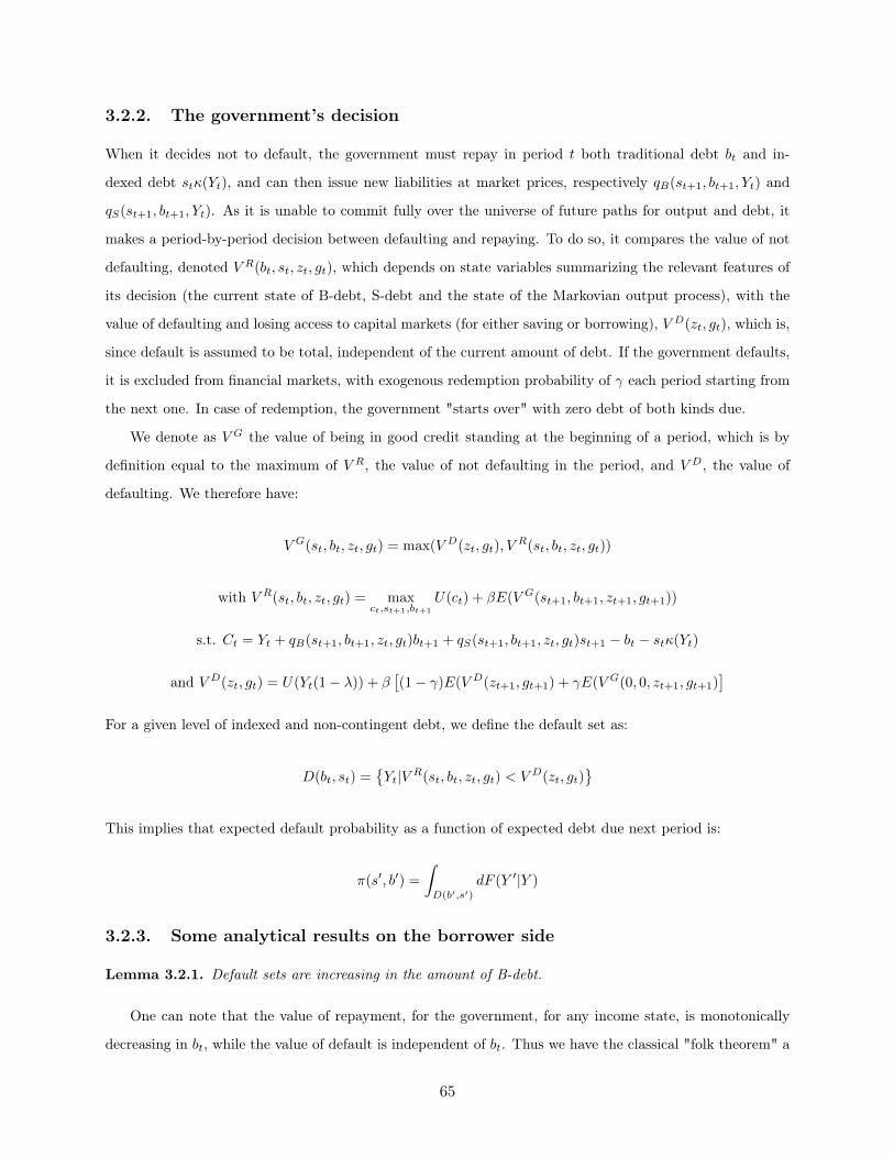
3.2.2. The government’s decision

When it decides not to default, the government must repay in period t both traditional debt bt and in-

dexed debt stκ(Yt), and can then issue new liabilities at market prices, respectively qB(st+1, bt+1, Yt) and

qS(st+1, bt+1, Yt). As it is unable to commit fully over the universe of future paths for output and debt, it

makes a period-by-period decision between defaulting and repaying. To do so, it compares the value of not

defaulting, denoted V R(bt, st, zt, gt), which depends on state variables summarizing the relevant features of

its decision (the current state of B-debt, S-debt and the state of the Markovian output process), with the

value of defaulting and losing access to capital markets (for either saving or borrowing), V D(zt, gt), which is,

since default is assumed to be total, independent of the current amount of debt. If the government defaults,

it is excluded from financial markets, with exogenous redemption probability of γ each period starting from

the next one. In case of redemption, the government "starts over" with zero debt of both kinds due.

We denote as V G the value of being in good credit standing at the beginning of a period, which is by

definition equal to the maximum of V R, the value of not defaulting in the period, and V D, the value of

defaulting. We therefore have:

V G(st, bt, zt, gt) = max(V D(zt, gt), VR(st, bt, zt, gt))

with V R(st, bt, zt, gt) = maxct,st+1,bt+1

U(ct) + βE(V G(st+1, bt+1, zt+1, gt+1))

s.t. Ct = Yt + qB(st+1, bt+1, zt, gt)bt+1 + qS(st+1, bt+1, zt, gt)st+1 − bt − stκ(Yt)

and V D(zt, gt) = U(Yt(1− λ)) + β[(1− γ)E(V D(zt+1, gt+1) + γE(V G(0, 0, zt+1, gt+1)

]For a given level of indexed and non-contingent debt, we define the default set as:

D(bt, st) ={Yt|V R(st, bt, zt, gt) < V D(zt, gt)

}This implies that expected default probability as a function of expected debt due next period is:

π(s′, b′) =

∫D(b′,s′)

dF (Y ′|Y )

3.2.3. Some analytical results on the borrower side

Lemma 3.2.1. Default sets are increasing in the amount of B-debt.

One can note that the value of repayment, for the government, for any income state, is monotonically

decreasing in bt, while the value of default is independent of bt. Thus we have the classical "folk theorem" a

65

la Eaton-Gersovitz-Arellano, that, for any given state of the world, repayment sets are shrinking in the level

of non-contingent B-debt: if Yt ∈ D(bt, st), then for bt > bt, Yt ∈ D(bt, st).

Lemma 3.2.2. Default sets are increasing in the amount of S-debt under limited investor liability.

The former result also applies to indexed debt, with a slight twist. As long as there is investor limited

liability, so that κ(Yt) ≥ 0, then: if Yt ∈ D(bt, st), then for st > st, Yt ∈ D(bt, st).

A number of classical results were derived in Arellano 2008 for the special case when shocks are i.i.d, so

that current output gives no information on future realizations of output, and the output costs of default

are zero. We turn to this special case to see which of these results are overturned in the presence of a mix

of S-debt and B-debt.

Lemma 3.2.3. Defaults only occur when the country faces capital outflows.

Proof. The proof is in appendix, section A.10.

The intuition is, as in Arellano, that, if there exists a contract with capital inflows, then for any income

state, entering said contract, consuming more today than the endowment (due to capital inflows), and keeping

the option to default next period, is strictly preferred to default and consumption of the endowment. Thus

there cannot be an income state where default is optimal and where capital inflows contracts are available.

Such a result cannot be overturned by the presence of indexed debt, as it simply depends on the increasing

nature of the utility function.

Separability of default and income Building on the no-capital-inflows result and on concavity of the

utility function, Arellano 2008 states that with i.i.d shocks, default sets are shrinking in the economy’s current

income. Since only contracts with capital outflows (net repayments) are available, and since the optimal

non-default contract with the low income level was available with the high income level, it is sufficient to

prove that the optimal non-default contract with the low income level yields lower utility than default in the

low income case.

Under non-contingent debt, it is the case because of the concavity of the utility function. In the presence of

indexed debt, however, this is no longer a necessity. Payments committed on by the country are themselves

decreasing in the current income, so that we could well have for Y1t < Y2t, u(Y1t − bt − stκ(Y1t)) > u(Y2t −

bt − stκ(Y2t)), depending on the form of indexation and the amount of indexed debt issued.

Sandleris, Saprizza, and Taddei 2011 seems to imply the result no longer holds. We can ask under what

conditions the Arellano results remains valid in the presence of indexed debt. Loosely speaking, it depends

66

on what decreases faster: payments, or the inverse of marginal utility.

To illustrate that point, let Y2 be just at the frontier of the default set, V D(Y2) = V R(b, s, Y2) (assuming

here that this implies Y2 ∈ D(b, s)). Let us also assume that non-contingent debt is 0, that default penalties

are zero. Let Y1 < Y2. We have, with obvious notations and s′i the utility maximizing level of debt chosen

with income Yi, because utility is maximized:

V R(s, Y1) = u(Y1 − sκ(Y1) + qSs′1) + βE(V G(s′1, Y

′)) ≥ u(Y1 − sκ(Y1) + qSs′2) + βE(V G(s′2, Y

′))

= u(Y1 − sκ(Y2) + qSs′2) + βE(V G(s′2, Y

′)) + [u(Y1 − sκ(Y1) + qSs′2)− u(Y1 − sκ(Y2) + qSs

′2)]

= u(Y1−sκ(Y2)+qSs′2)+u(Y2)−u(Y2−sκ(Y2)+qSs

′2)+βE(V D(Y ′))+[u(Y1−sκ(Y1)+qSs

′2)−u(Y1−sκ(Y2)+qSs

′2)]

because Y2 is at the frontier of the default set

= u(Y1)+βE(V D(Y ′))+[u(Y2)−u(Y1)]+[u(Y1−sκ(Y2)+qSs′2)−u(Y2−sκ(Y2)+qSs

′2)]+[u(Y1−sκ(Y1)+qSs

′2)−u(Y1−sκ(Y2)+qSs

′2)]

= V D(Y1)+[u(Y2)−u(Y1)]+[u(Y1−sκ(Y2)+qSs′2)−u(Y2−sκ(Y2)+qSs

′2)]+[u(Y1−sκ(Y1)+qSs

′2)−u(Y1−sκ(Y2)+qSs

′2)]

The first term in bracket is positive, the second term is negative, and the third is positive. We also know

that, because there cannot be any capital inflows when the default set is non-empty, −sκ(Y2) + qSs′2 < 0,

and, by concavity of the utility function, [u(Y2)−u(Y1)]+[u(Y1−sκ(Y2)+qSs′2)−u(Y2−sκ(Y2)+qSs

′2)] < 0.

However, we conjecture that by concavity of the utility function, if s is large enough or κ steep enough, the

last term could be large enough to make the overall sum positive. In other words, with large enough amounts

of indexed debt, it is possible to construct a contract such that with output Y1, the country strictly prefers

repayment to default even if with higher output it prefers default to repayment.

The proposition below generalizes the result.

Proposition 3.2.4. There exists an amount S such that default sets are shrinking in income when the

amount of S-debt is below, and increasing in income when it is above

Proof. See appendix, section A.11.

3.2.4. The lenders’ problem

We now turn to the lender side of the environment, which, in equilibrium, will endogenously determine

the respective prices of S-debt and B-debt. The representative investor exhibits decreasing absolute risk

aversion utility, of the form vL(cLt) =c1−ψLt

1−ψ . International lenders have aggregate wealth Wt, and they

67

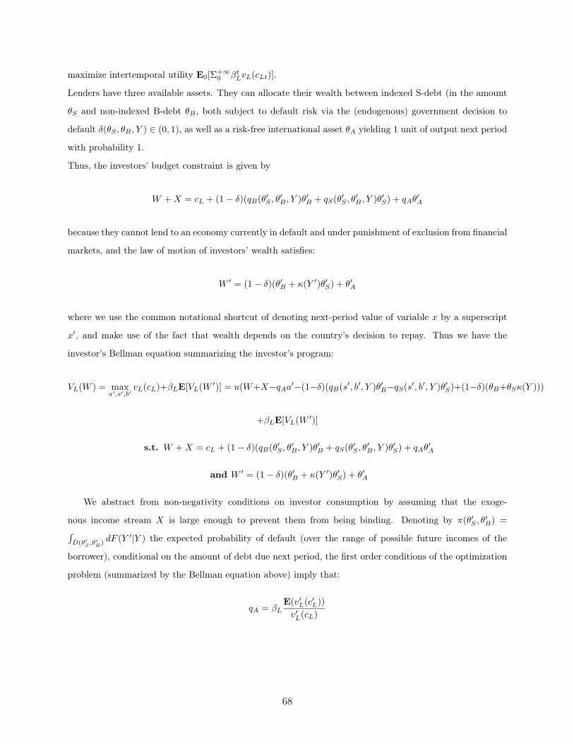
maximize intertemporal utility E0[Σ+∞0 βtLvL(cLt)].

Lenders have three available assets. They can allocate their wealth between indexed S-debt (in the amount

θS and non-indexed B-debt θB , both subject to default risk via the (endogenous) government decision to

default δ(θS , θB , Y ) ∈ (0, 1), as well as a risk-free international asset θA yielding 1 unit of output next period

with probability 1.

Thus, the investors’ budget constraint is given by

W +X = cL + (1− δ)(qB(θ′S , θ′B , Y )θ′B + qS(θ′S , θ

′B , Y )θ′S) + qAθ

′A

because they cannot lend to an economy currently in default and under punishment of exclusion from financial

markets, and the law of motion of investors’ wealth satisfies:

W ′ = (1− δ)(θ′B + κ(Y ′)θ′S) + θ′A

where we use the common notational shortcut of denoting next-period value of variable x by a superscript

x′, and make use of the fact that wealth depends on the country’s decision to repay. Thus we have the

investor’s Bellman equation summarizing the investor’s program:

VL(W ) = maxa′,s′,b′

vL(cL)+βLE[VL(W ′)] = u(W+X−qAa′−(1−δ)(qB(s′, b′, Y )θ′B−qS(s′, b′, Y )θ′S)+(1−δ)(θB+θSκ(Y )))

+βLE[VL(W ′)]

s.t. W +X = cL + (1− δ)(qB(θ′S , θ′B , Y )θ′B + qS(θ′S , θ

′B , Y )θ′S) + qAθ

′A

and W ′ = (1− δ)(θ′B + κ(Y ′)θ′S) + θ′A

We abstract from non-negativity conditions on investor consumption by assuming that the exoge-

nous income stream X is large enough to prevent them from being binding. Denoting by π(θ′S , θ′B) =∫

D(θ′S ,θ′B)dF (Y ′|Y ) the expected probability of default (over the range of possible future incomes of the

borrower), conditional on the amount of debt due next period, the first order conditions of the optimization

problem (summarized by the Bellman equation above) imply that:

qA = βLE(v′L(c′L))

v′L(cL)

68

and, when the economy is not in default in the current period (δ = 0), we have, for non-contingent debt:

qB(θ′S , θ′B , Y ) = βL

E((1− δ′)v′L(c′L))

v′L(cL)

= βLE(v′L(c′L))E(1− δ′)

v′L(cL)+ βL

Cov(1− δ′, v′L(c′L))

v′L(cL)= qA(1− π(θ′S , θ

′B)) + βL

Cov(1− δ′, v′L(c′L))

v′L(cL)

With such investor preferences, default risk affects the pricing of B-debt by an additional channel,

compared to the traditional case of risk-neutral investor: not only is the expected return on debt scaled

down by default probability, but default-induced volatility in portfolio returns requires excess risk premia

for investors.

The price of non-contingent debt, in that case, is the sum of a risk-neutral price (expected probability

of default times price of riskless asset), and a term reflecting the covariance between marginal utility of

consumption and the asset’s payoff. The covariance term is negative, since the asset pays a return only when

not in default, i.e. in periods when lender’s wealth and thus consumption is higher, and marginal utility is

lower (see Lizarazo 2013 and Borri and Verdelhan 2011 for a discussion of this result, which goes a long way

in explaining empirical spreads for emerging markets).

We also have, when the economy is not in default in the current period, for indexed debt:

qS(θ′S , θ′B , Y ) = βL

E(κ(Y ′)(1− δ′)v′L(c′L))

v′L(cL)

=E(v′L(c′L))

v′L(cL)((1− π(θ′S , θ

′B))E(κ(Y ′)) + Cov(1− δ′, κ(Y ′))) + βL

Cov((1− δ′)κ(Y ′), v′L(c′L))

v′L(cL)

= qA(1− π(θ′S , θ′B)) + qACov(1− δ′, κ(Y ′)) + βL

Cov((1− δ′)κ(Y ′), v′L(c′L))

v′L(cL)

Indexed debt, on the other hand, will be affected both by excess risk premia arising from default probability,

and by risk premia arising from the volatility of payoffs themselves in non-default cases.

For indexed S-debt, the price is thus the sum of three terms. The first is a simple adjustment of the risk-free

asset’s price by the default probability. The second is a term reflecting the upwards adjustment of payoffs of

indexed debt conditional on repayment (payments κ(Y ′) are increasing in Y ′, and if the asset is less likely

to default when Y ′ is high, then Cov((1 − δ′), κ(Y ′)) > 0). The third term reflects the covariance between

marginal utility of consumption and the asset’s payoff. Since the asset pays a return only when not in

default, i.e. when consumption of the lender is higher, and marginal utility of the lender is lower, this term

is negative. Moreover, the latter term will be larger (in absolute value) than in the non-contingent case,

since payoffs (1− δ′)κ(Y ′) are not only binary (default/non-default), but also increasing in Y , making them

even more negatively correlated with the lender’s marginal utility of wealth, and requiring higher excess risk

69

premia than bonded non-contingent B-debt to compensate for the additional volatility. We prove this in the

below lemma.

Lemma 3.2.5. When the default set is empty, indexed debt has a lower price than non-contingent debt.

Proof. See appendix, section A.12.

3.2.5. Definition of equilibrium

We define the recursive equilibrium of the economy as a situation in which the government optimally chooses

its repayment decision and new debt issuance conditional on asset prices which reflect the representative

lender’s necessary risk compensation.

Definition 3.2.1. Recursive equilibrium A recursive competitive equilibrium in this setup corresponds to:

1. A decision rule for the government on (a) default decision, and (b) indexed S-debt and non-contingent

B-debt issuance, maximizing the program of the government subject to equilibrium bond prices, and

such that consumption satisfies the resource constraint.

2. Equilibrium bond prices satisfying the first-order conditions of the maximization program of the risk-

averse lenders, i.e. pricing conditions for risk-free assets, B-debt, and S-debt compensating investors

for default risk and payoff volatility.

3. Individual bond-buying decisions consistent with debt issuance, i.e. market clearing for both types of

debt : θ′S = s′ and θ′B = b′ for b′, s′ ≥ 0

4. The law of motion for wealth, consistent with government repayment decisions and contractual payoffs

on the bonds.

3.2.6. Optimal debt structure

A key question is whether in equilibrium, we expect the government to optimally issue both types of debt.

This section, in a way, parallels the methodology of Arellano and Ramanarayanan 2012 who show that an

interior solution (to their problem of debt maturity mix) equates the "hedging" benefits of long-term debt

(larger than for short-term debt) with its "incentives" costs (higher than short-term debt). The results we

derive in this section assume i.i.d. shocks to output to shut down the output persistence effects on prices of

indexed debt and focus on the borrower’s incentives.

Similarly, here, there are hedging benefits of indexed debt. However, if lenders are risk-neutral, the higher

relative costs are on the non-contingent debt side rather than on the indexed side, so that no interior solution

can exist. To counteract the strength of both incentive effects and hedging benefits, risk-aversion of the lender

70

is necessary.

Assume differentiability of bond prices and value functions. Let us first suppose that there is indeed an

interior solution to the borrower’s problem. Using the envelope theorem, the first-order condition to the

government’s problem with respect to non-contingent debt issuance b′ then writes as:

U ′(C)(qB +∂qB∂b′

b′ +∂qS∂b′

s′) = β

∫D(b′,s′)

∂V G

∂b′dF (Y ′|Y ) = β

∫D(b′,s′)

U ′(C ′)dF (Y ′|Y )

Similarly, the first-order condition to the government’s problem with respect to contingent debt issuance s′

writes:

U ′(C)(qS +∂qB∂s′

b′ +∂qS∂s′

s′) = β

∫D(b′,s′)

∂V G

∂s′dF (Y ′|Y ) = β

∫D(b′,s′)

U ′(C ′)κ(Y ′)dF (Y ′|Y )

The first-order conditions only take into account the marginal effect of an additional unit of borrowing on the

value of repayment next period, and not on the value of default or on the default threshold. This is because,

as shown by Arellano and Ramanarayanan 2012 (footnote 7, p.201), at the margin between repayment and

default, the values of repayment and default are equal, and thus a small change in b′ or in s′, even if it affects

the repayment decision at the margin next period, has a zero marginal effect on the value function today

(this is akin to an "envelope condition" at the margin between repayment and non repayment).

Dividing the first-order-conditions by qB and qS , respectively, and using the lender’s first-order-condition,

we then have:

U ′(C)(1 +∂qB∂b′

b′

qB+∂qS∂b′

s′

qB) =

β∫D(b′,s′)

U ′(C ′)dF (Y ′|Y )

qA(1− π(s′, b′)) + βLCov(1−δ′,v′L(c′L))

v′L(cL)

and

U ′(C)(1 +∂qB∂s′

b′

qS+∂qS∂s′

s′

qS) =

β∫D(b′,s′)

U ′(C ′)κ(Y ′)dF (Y ′|Y )

qA(1− π(s′, b′)) + qACov(1− δ′, κ(Y ′)) + βLCov((1−δ′)κ(Y ′),v′L(c′L))

v′L(cL)

Risk-neutral lenders Now first examine the case when lenders are risk-neutral (v′L(c′L) = 0). Note

that:∫D(b′,s′) U

′(C′)dF (Y ′|Y )

(1−π(s′,b′)) = E(U ′(C ′)|D).

Also note that the expected payment on indexed debt, conditional on no-default, is:

E(κ(Y ′)|D) =

∫D

κ(Y ′)dF (Y ′|Y )

1− π(s′, b′)=

Cov(1− δ′, κ(Y ′)) + E(κ(Y ′))E(1− δ)1− π(s′, b′)

=Cov(1− δ′, κ(Y ′))

(1− π(s′, b′))+ 1

We thus have, after some manipulations:

U ′(C)(1 +∂qB∂b′

b′

qB+∂qS∂b′

s′

qB) =

βE(U ′(C ′)|D)

qA

71

and

U ′(C)(1 +∂qB∂s′

b′

qS+∂qS∂s′

s′

qS) =

E(U ′(C ′)|D)

qA

βE(U ′(C ′)κ(Y ′)|D)

E(U ′(C ′)|D)(1 + Cov(1−δ′,κ(Y ′))(1−π(s′,b′)) )

U ′(C)(1 +∂qB∂s′

b′

qS+∂qS∂s′

s′

qS) =

E(U ′(C ′)|D)

qA

βE(U ′(C ′)κ(Y ′)|D)

E(U ′(C ′)|D)E(κ(Y ′)|D)

Taking the ratio of the first-order conditions then yields:

(1 + ∂qB∂s′

b′

qS+ ∂qS

∂s′s′

qS)

(1 + ∂qB∂b′

b′

qB+ ∂qS

∂b′s′

qB)

=βE(U ′(C ′)κ(Y ′)|D)

E(U ′(C ′)|D)E(κ(Y ′)|D)

The right-hand-side term is below 1, and represents the "hedging benefit" of indexed debt: it comes from

the fact that κ(Y ′) is high when output is high, and thus when marginal utility of consumption for the

borrower is low (Cov(U ′(C ′), κ(Y ′)) < 0). The left-hand-side term is the relative cost effect: it measures the

relative sensitivity of debt prices to changes in the levels of each kind of debt. However, this cost term, with

risk-neutral lenders, is actually also favorable to indexed debt. It is above 1, meaning that debt prices are

more (in absolute value, in negative terms) sensitive to changes in the level of non-contingent B-debt than

to changes in the level of contingent S-debt. This is because, for risk-neutral lenders, the effect of a marginal

increase in debt on prices only goes through the increased probability of default; and a marginal increase

in S-debt has a lesser effect on increased default probability than a marginal increase in B-debt, due to the

indexed character of S-debt which dampens default risk.

Therefore the above equality is actually a contradiction, and it is not possible to "equate" the relative benefits

of indexed debt and its relative costs. The interior solution does not exist, and a corner solution with only

indexed debt is preferred.

Risk-averse lenders Thus, having risk-averse lenders is a necessary condition for an interior mix of

indexed S-debt and non-contingent B-debt. Starting again from the normalized first-order conditions, but

keeping the risk-aversion term:

U ′(C)(1 +∂qB∂b′

b′

qB+∂qS∂b′

s′

qB) =

β∫D(b′,s′)

U ′(C ′)dF (Y ′|Y )

qA(1− π(s′, b′)) + βLCov(1−δ′,v′L(c′L))

v′L(cL)

and

U ′(C)(1 +∂qB∂s′

b′

qS+∂qS∂s′

s′

qS) =

β∫D(b′,s′)

U ′(C ′)κ(Y ′)dF (Y ′|Y )

qA(1− π(s′, b′)) + qACov(1− δ′, κ(Y ′)) + βLCov((1−δ′)κ(Y ′),v′L(c′L))

v′L(cL)

72

After similar manipulations:

U ′(C)(1 +∂qB∂b′

b′

qB+∂qS∂b′

s′

qB) =

βE(U ′(C ′)|D)

qA + βLCov(1−δ′,v′L(c′L))

v′L(cL)(1−π(s′,b′))

and:

U ′(C)(1 +∂qB∂s′

b′

qS+∂qS∂s′

s′

qS) =

E(U ′(C ′)|D)

qA + βLCov((1−δ′)κ(Y ′),v′L(c′L))

v′L(cL)(1−π(s′,b′))

βE(U ′(C ′)κ(Y ′)|D)

E(U ′(C ′)|D)E(κ(Y ′)|D)

Taking the ratio of the FOC yields:

(1 + ∂qB∂s′

b′

qS+ ∂qS

∂s′s′

qS)

(1 + ∂qB∂b′

b′

qB+ ∂qS

∂b′s′

qB)

=qA + βL

Cov((1−δ′)κ(Y ′),v′L(c′L))

v′L(cL)E(κ(Y ′)|D)(1−π(s′,b′))

qA + βLCov(1−δ′,v′L(c′L))

v′L(cL)(1−π(s′,b′))

E(U ′(C ′)κ(Y ′)|D)

E(U ′(C ′)|D)E(κ(Y ′)|D)

When lenders are risk-averse, a marginal increase in indexed S-debt improves current consumption of the

borrower by less than a marginal increase in non-indexed B-debt, because of its lower price, itself the result

of the additional volatility in consumption for the lenders that it creates. This is all the truer when lenders

are more risk averse.

Without default risk In the specific case with no default risk, the above optimality condition reduces

to:qA

qA + βLCov(κ(Y ′),v′L(c′L))

v′L(cL)E(κ(Y ′))

(1 + ∂qB∂s′

b′

qS+ ∂qS

∂s′s′

qS)

(1 + ∂qB∂b′

b′

qB+ ∂qS

∂b′s′

qB)

=E(U ′(C ′)κ(Y ′))

E(U ′(C ′))E(κ(Y ′))

and we note that if, for example, indexed debt indeed achieves full insurance (constant U ′(C ′)), then the

right hand side of the equation is 1. The left-hand-side, however, tends to be above 1 (assuming comparable

and small elasticities of debt prices to the level of debt in the non-default zone), because of the lower price

of indexed debt (by lemma 3.2.5). This suggests that the full-indexation solution is not optimal: reducing

indexed debt by a small amount and substituting it by non-contingent debt improves current consumption,

and would go in the direction of equating the higher costs of indexed debt (equivalently, its lower price,

qA + βLCov(κ(Y ′),v′L(c′L))v′L(cL)E(κ(Y ′)) < qA) with its hedging benefits.

We summarize the results in the proposition below.

Proposition 3.2.6. In equilibrium, with i.i.d. shocks, in periods where it has access to capital markets, the

government only issues S-debt if lenders are risk-neutral. With risk-averse lenders, an interior solution with

a "sovereign debt-equity mix" is optimal if there is no default risk and full insurance when the government

issues only S-debt. The share of B-debt will be increasing in lender risk-aversion.

73

3.3. Calibration and implementation of the algorithm

3.3.1. A detrended version

For the calibration, it is necessary for stationarity to work with a normalized, detrended version of the model.

We had:

V G(st, bt, gt, zt) = max(V D(gt, zt), VR(st, bt, gt, zt))

with V R(st, bt, gt, zt) = maxct,st+1,bt+1

U(ct) + βE(V G(st+1, bt+1, gt+1, zt+1))

s.t. Ct = Yt + qB(st+1, bt+1, Yt)bt+1 + qS(st+1, bt+1, Yt)st+1 − bt − stκ(Yt)

and V D(gt, zt) = U(Yt(1− λ)) + β[(1− γ)E(V D(gt+1, zt+1) + γE(V G(0, 0, gt+1, zt+1)

]We further assume that indexed payments only depend on detrended growth, κ(Yt) = κ(gt, zt), as is the case

in most indexation formulas that do not include level conditions. We denote by xt = xtµgΓt−1

the detrended

value of variable x, using the known at t t − 1-value of the growth trend. Then, because of the linearities

built in the utility function and the decision rule (and thus in the prices for both types of debt), the value

functions are homogeneous of degree 1− σ. We have that:

V R(st, bt, gt, zt) = (µgΓt)1−σV R(st, bt, zt, gt)

and

V D(gt, zt) = (µgΓt)1−σ ˆV D(zt, gt)

so thatV G(st, bt, gt, zt)

(µgΓt)1−σ = V G(st, bt, zt, gt) = max( ˆV D(zt, gt), V R(st, bt, zt, gt))

with:

with V R(st, bt, zt, gt) = maxst+1,bt+1

(µgΓt−1)1−σ(ezt gtµg − bt − stκ(Yt) + qB( ˆst+1, ˆbt+1) ˆbt+1gt + qS( ˆst+1, ˆbt+1) ˆst+1gt)1−σ

1− σ

+β(µgΓt)1−σE(V G( ˆst+1, ˆbt+1, zt+1, gt+1))

and( ˆV D(zt, gt) =(µgΓt−1)1−σ((1− λ)(eztgt)

1−σ

1− σ+β(µgΓt)

1−σ[(1− γ)E( ˆV D(zt+1, gt+1)) + γE(V G(0, 0, zt+1, gt+1)

]

74

3.3.2. Calibration and parametrization

The literature on sovereign debt has made a habit of calibrating most models to Argentinian data, with

Argentina taken to be the quintessential serial defaulter. Moreover, since Argentina, up until recently, was

one of the only countries to have ever issued GDP-indexed debt, it appeared fitting to choose that example

when studying the property of GDP-linked instruments.

We prefer to focus on Greece, for several reasons. While Argentina regained access to financial markets

in April 2016, Greece remains in a dire public debt situation, and may require a new haircut on official

creditors to return to a sustainable debt ratio. Some, including a former Greek finance minister, have

proposed swapping part of its current debt held by Euro area member-States with GDP-linked instruments.

Moreover, Greece also issued GDP-indexed warrants as part of its 2011-12 restructuring.

The coefficient of risk-aversion for the borrower is set to σ = 2, as is standard in the literature. The

probability of redemption is set at 17% as in Benjamin and M. L. Wright 2009, the baseline (quarterly)

interest rate is 1% as in M. Aguiar and Gopinath 2006, and the discount rate has a low value of 0.8. The

cost of defaulting is set at 2% of output.

For the output process, we calibrate the data using OECD data for the Greek economy. We estimate a

process for output for Greece, in the fashion of M. Aguiar and Gopinath 2006, to have either a stochastic

trend or only transitory shocks.

First, we use data over the whole period 1970-2015, take the log of output, detrend it using a linear trend,

and find that the autocorrelation coefficient when fitting an AR(1) process to the log of detrended GDP is

ρz = 0.959, with a standard deviation of shocks of σz = 2.71%. We use these figures for a model with only

z shocks.

The alternative is a model with shocks to trend g and no transitory shocks. We plot the path of real GDP

for Greece in figure 3.1. The clear decline in levels after the 2007-8 crisis points to a stochastic trend. We

plot below a kernel density estimate of Greek growth data (quarterly) in figure 3.2, as well as a histogram

of the actual distribution. It appears that Greek GDP growth (quarterly) for Greece is well-approximated

by a simple, i.i.d normal distribution. However, this simple cross-section over time series data does not

account for growth persistence. Growth appears to have become much more persistent since 1995 (see fig.

3.3: the autocorrelation coefficient is almost 0 over the period 1970-1995, but close to 0.4 over the last 20

years. We focus on this later period for our model with shocks to trend, conjecturing that data quality

issues for the previous 25 years may account for this discrepancy. We then use a process with persistence

parameter ρg = 0.4, µg = 0.023 and standard deviation of 3%. We then discretize the shocks (either

transitory or permanent) into 25 states using Tauchen’s quadrature procedure, and define a discrete-grid

Markov transition probability matrix (Tauchen and Hussey 1991).

75

Figure 3.1: Greek real GDP at constant 2010 prices, 1970-2014

Figure 3.2: Greek GDP growth, kernel density estimation, 1970-2014

3.3.3. Fixed exogenous shares of debt

As a first step, a shortcut to avoid having too many state variables (thus making the model solvable) is to

specifiy ex ante that each unit of debt actually entails a bundle, with a fixed share θ of indexed debt, and

a share 1 − θ of traditional non-contingent debt. The price of each unit of this bundle is then a weighted

average of the expected net present values of payoffs on non-contingent debt and on indexed debt. We can

thus summarize the current state by a single state variable total amount of debt.

We adopt the following algorithm as the structure of our solution method:

1. Start with initial guess for price of debt bundle q

76

Figure 3.3: Greek GDP growth, 1970-2014

2. Start with initial guess for value functions V D and V R

3. Iterate value function over policy functions (summarized by total amount of debt a corresponding to

b = (1− θ)a and s = θa for a given bundle price until convergence

4. Compute debt bundle price given optimal default rule and optimal issuance q′, as a weighted average

of the expected net present values of payoffs on non-contingent debt and on indexed debt

5. Update debt bundle price until it converges q∞S

We are able to have a relatively fine grid of 400 levels for the asset bundle quantity. We perform

comparative statics on the share of indexation (a la Durdu 2009) in appendices H and I, where we also make

the assumption of risk-neutral lenders (since risk aversion is only needed for an interior solution when the

decision to issue both types of debt is endogenous). Matlab codes for the simulations are available at the

following address.

We show that a higher share of indexation (varying from 0 to 50% in our simulations) reduces the occurrences

of default, thus increasing the prices of both types of debt. The price of non-contingent debt, for high

indexation shares, thus becomes almost independent from current income or from the amount of debt issued

next period, while the price of indexed debt is mainly determined by the conditional expectation of output

next period given its level today, as seen in figures 3.4 and 3.5 below, which show both prices for the case of

stochastic trend shocks at a 50% share of indexed debt.

However, the change in steepness of the debt price function is of a larger amplitude when shocks are

to trend growth (appendix H) rather than transitory (appendix I). Indeed, in the case of transitory shocks,

77

Figure 3.4: 50% share of indexed debt, risk-neutral lenders: price of non-contingent debt

Figure 3.5: 50% share of indexed debt, risk-neutral lenders: price of contingent debt

the interest rate schedule is already very steep with only non-contingent debt, as the difference between

value functions of good and bad standing is then mostly a function of the debt burden rather than the

income process. On the contrary, when shocks are to trend, the difference of the value functions is itself

very sensitive to the income shock, which affects the whole trajectory of future income levels. Therefore,

introducing indexed debt in this setting, by partially decoupling default decisions from current realizations

78

of the shock, increases the steepness of the interest rate schedule by a wider margin than under transitory

shocks.

3.3.4. Endogenous shares of debt

We then turn to our actual general equilibrium model, with endogenous shares of indexed and non-contingent

debt, and risk-averse pricing. A significant computational issue arises when trying to implement the algo-

rithm: counting the current value of both technology processes (zt and gt), the amount of indexed debt st,

and the amount of non-contingent debt bt, we have at least four state variables; five if we add an independent

variable for lender’s consumption to introduce a closed-form version of risk aversion. If we try to have a

fine enough partition of the state space, this is computationally costly, and not solvable via the traditional

space-grid method.

We successively shut down either transitory or permanent shocks, to reduce the dimensionality of the prob-

lem, and adopt a less fine partition of the asset space for both types of debt (20 values for each type of debt

instead of 400 for the "bundled-debt" case).

We use a reduced form for the stochastic discount factor of the lender. Following Arellano and Rama-

narayanan 2012, the prices of sovereign B-bonds and S-bonds are determined according to a no-arbitrage

condition which incorporates a stochastic discount factor that only depends on the current shock and its

variance, and a given "market price of risk". This one-factor model for the stochastic discount factor, inspired

from J. H. Cochrane and Piazzesi 2009, defines the investor’s discount factor as:

mt+1 =1

1 + r− ν(yt+1 −Et(yt + 1))

This creates a (negative) correlation between the investor’s stochastic discount factor and the payoffs on

indexed and non-contingent debt, thus generating a reduced form risk premium1.

We adopt the following algorithm as the structure of our solution method:

1. Start with initial guess for indexed bond price qS

2. Make an initial guess for non-contingent bond price qB

3. Start with initial guess for value functions V D and V R

4. Iterate value function over policy functions for given bond prices until convergence

1These simplifications are made in order to obtain a computationally manageable solution method. The cost interms of precision of this methodology is probably significant, but assessing this accuracy loss is beyond the scope ofthis work.

79

5. Compute non-contingent bond price given optimal decision rules and issuance, as well as stochastic

discount factor process q′B

6. Repeat from 3 with updated non-contingent bond price, until it converges q∞B

7. Compute indexed bond price given optimal decision rules and issuance, stochastic discount factor

process q′S

8. Repeat from 2 with updated indexed bond price until it converges q∞S

The relevant Matlab code is available at the following address for risk-neutral lenders, and at this address

for risk-averse pricing.

Risk-neutral lenders

Shocks to trend We first start with the case of risk-neutral lenders (defining the stochastic discount

factor matrix as 11+r ×I). Focusing on the case with shocks to trend (which, given low persistence of growth,

is closest to the i.i.d. shocks case studied in our analytical derivation), we follow our solution method,

and find first that the country issues, in total, a larger amount of total debt than in an equilibrium where

only non-contingent debt is available. Moreover, the country chooses to issue a zero or low amount of non-

contingent debt (locating itself at the three lowest absolute values of our partition of the asset space for

non-contingent debt).

The country selects in most states of the world a bundle with c. 22-25% of endowment in indexed debt

and 5% in non-contingent debt, except for the highest income shocks case, where it issues, indeed, a zero

amount of non-contingent debt, because the expected payoff on indexed debt is higher (due to persistent

growth shocks) and thus S-debt has an even higher relative price, making it more valuable to issue (while

the reduction in default risk effect is small).

We also find that in that case, default becomes almost independent from the actual realization of output

shocks (the default space is almost the same at the highest and lowest endowment shocks). For example, we

plot in figures 3.6, 3.7, and 3.8 the respective default spaces for various levels of indexed and non-indexed debt

at the lowest, average, and highest endowment shocks, and observe that they are almost exactly the same.

This is, in a way, a generalization of our initial observation in this chapter that with indexed debt, since

payments are lower in bad states of the world, the government can issue debt up to a defined "debt limit",

above which it always defaults and under which it never does (remember our observation that under pure

indexed debt, S < S = λκ ). Issuing indexed debt only under growth shocks and risk-neutral lenders enables,

as in Faria 2007, separability of the value function into income and a component that only depends on the

level of debt. The results showing the prices of indexed and non-contingent debt depending on both the

80

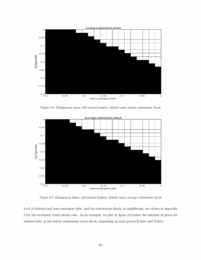
Figure 3.6: Endogenous share, risk-neutral lenders: default cases, lowest endowment shock

Figure 3.7: Endogenous share, risk-neutral lenders: default cases, average endowment shock

level of indexed and non-contingent debt, and the endowment shock, in equilibrium, are shown in appendix

J for the stochastic trend shocks case. As an example, we plot in figure 3.9 below the schedule of prices for

indexed debt at the lowest endowment trend shock, depending on next period B-debt and S-debt.

81

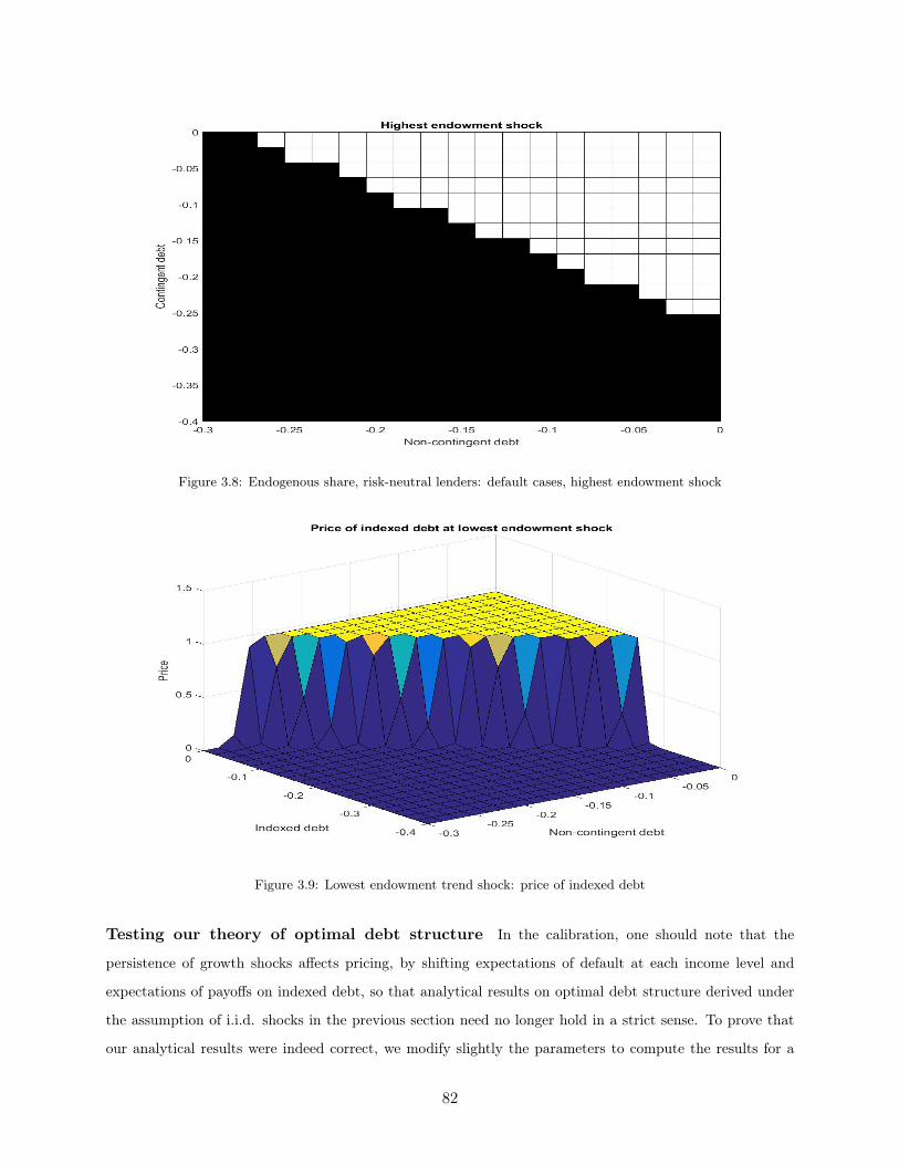
Figure 3.8: Endogenous share, risk-neutral lenders: default cases, highest endowment shock

Figure 3.9: Lowest endowment trend shock: price of indexed debt

Testing our theory of optimal debt structure In the calibration, one should note that the

persistence of growth shocks affects pricing, by shifting expectations of default at each income level and

expectations of payoffs on indexed debt, so that analytical results on optimal debt structure derived under

the assumption of i.i.d. shocks in the previous section need no longer hold in a strict sense. To prove that

our analytical results were indeed correct, we modify slightly the parameters to compute the results for a

82

persistence parameter ρg = 0 (i.i.d. growth shocks), and find indeed that for risk-neutral lenders, the country

chooses the maximum amount of indexed debt and a zero amount of non-contingent debt at all income states.

Transitory shocks The results (default spaces and prices) in the transitory shocks case are shown in

appendix K. Default tends to be less likely overall, and thus a higher burden of debt is supported. The

optimal policy involves a more balanced mix of both types of debt, as the country chooses a bundle with

c. 10% of endowment in indexed debt and 20% non-contingent debt in the lowest endowment shocks states

(because contingent debt has a lower price due to low output expectations); c. 10% in non-contingent

debt and 20% in indexed debt in intermediary states (because there is some likelihood of default, making

non-contingent debt less valuable); and c.15% of each type of debt in higher endowment states (where the

likelihood of default is low, but the price of indexed debt is high due to high growth expectations).

This is because under transitory shocks, even risk-neutral prices of indexed debt become very correlated to

the current state of the economy (more so than prices of non-contingent debt), thus justifying borrowing

more on non-contingent terms in times of low shocks. As an example, we plot in figure 3.10 and figure

3.11 below the schedule of prices for indexed debt at the lowest and highest endowment transitory shocks,

depending on next period B-debt and S-debt.

Figure 3.10: Lowest endowment transitory shock: price of indexed debt

Risk-averse lenders

83

Figure 3.11: Highest endowment transitory shock: price of indexed debt

Trend shocks With risk-averse lenders and trend shocks, the government issues a lower amount of both

types of debt, as the benefit of staying in good standing is reduced by higher borrowing costs, thus triggering

default in more income-debt states, and constraining the amount of borrowing as a result. Therefore, the

total amount of debt issued is closer to 15% of endowment, compared to 30% with risk-neutral lenders.

Moreover, the government will indeed choose, in our simulations, to issue more non-contingent debt relative

to indexed debt compared to the risk-neutral case, as suggested by our analytical results, because of the

lower price of indexed debt arising from risk premia (for given expectations of output next period). The

magnitude of this effect is partly muted because, due to the sizable reduction in overall borrowing arising

from risk aversion, the government issues more debt in higher states of the world and thus has incentives to

take advantage of high indexed debt prices. We do find, nonetheless, that the optimal amount of debt issued

in lower states of the world is c.8% of endowment in each type of debt, indexed and non-contingent.

We plot in figures 3.12, and 3.13 the respective default spaces for various levels of indexed and non-indexed

debt at the lowest and highest endowment shocks. The resulting prices for contingent and non-contingent

debt, as well as the equilibrium default space as a function of the amount of indexed debt, non-indexed debt,

and income, are shown in appendix L.

Transitory shocks The results in the transitory shocks case are shown in appendix M. They show a

higher burden of debt is supported in equilibrium at a given investor risk aversion than in the case with

trend shocks.

84

Figure 3.12: Endogenous share, risk-averse lenders: default cases, lowest endowment trend shock

Figure 3.13: Endogenous share, risk-averse lenders: default cases, highest endowment trend shock

The optimal policy involves, in most endowment states, a high share of non-contingent debt (c. 10-12% of

output) and a lower share of indexed debt (c. 5%), for reasons similar to the risk neutral case; moreover,

the price of indexed debt is lower in most endowment shocks states due to its high correlation with investor

wealth, making it less valuable to issue for the borrower. The default spaces are shown for high and low

transitory shocks in figures 3.14 and 3.15.

85

Figure 3.14: Endogenous share, risk-averse lenders: default cases, lowest endowment transitory shock

Figure 3.15: Endogenous share, risk-averse lenders: default cases, highest endowment transitory shock

86

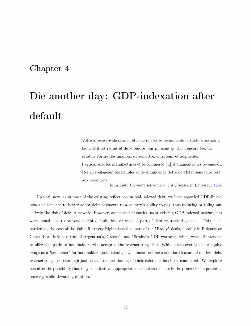
Chapter 4

Die another day: GDP-indexation after

default

Votre altesse royale sera en état de relever le royaume de la triste situation à

laquelle il est réduit et de le rendre plus puissant qu’il n’a encore été, de

rétablir l’ordre des finances, de remettre, entretenir et augmenter

l’agriculture, les manufactures et le commerce [...] d’augmenter les revenus du

Roi en soulageant les peuples et de diminuer la dette de l’Etat sans faire tort

aux créanciers.John Law, Première lettre au duc d’Orléans, in Levasseur 1854

Up until now, as in most of the existing reflections on real-indexed debt, we have regarded GDP-linked

bonds as a means to better adapt debt payments to a country’s ability to pay, thus reducing or ruling out

entirely the risk of default ex ante. However, as mentioned earlier, most existing GDP-indexed instruments

were issued, not to prevent a debt default, but ex post, as part of debt restructuring deals. This is, in

particular, the case of the Value Recovery Rights issued as part of the "Brady" deals, notably in Bulgaria or

Costa Rica. It is also true of Argentina’s, Greece’s, and Ukraine’s GDP warrants, which were all intended

to offer an upside to bondholders who accepted the restructuring deal. While such sovereign debt-equity

swaps as a "sweetener" for bondholders post-default, have almost become a standard feature of modern debt

restructurings, no thorough justification or questioning of their existence has been conducted. We explore

hereafter the possibility that they constitute an appropriate mechanism to share in the proceeds of a potential

recovery while thwarting dilution.

87

4.1. Financing, forgiving, or indexing a debt overhang?

Aligning creditors’ and debtors’ interests? It has been suggested that GDP-linked instruments

in the aftermath of a default are a solution to align the interests of creditors and those of borrowers. The

intuition is that, if creditor’s claims (at face value) are larger than the country’s ability to pay, it may be

optimal to forgive a share of the debt in order to recover as much as possible. However, doing so implies

renouncing to the option value of a future recovery: in that context, GDP-indexed claims may provide an

efficient restructuring tool.

Indeed, in the context of the debt overhang literature, legacy debt acts as a "tax on the marginal unit of

output", so that the country’s incentives to grow are muted when it inherits a large stock of "legacy" debt.

When a country cannot repay its debt, creditors face a trade-off between forgiving a share of their debt (thus

improving a country’s incentives to grow) and refinancing debt by betting on a country’s eventual recovery

rather than taking losses upfront (Krugman 1988). Indexed debt is a means to formalize the later choice,

by explicitly stating that existing creditors convert their claims into claims on a possible positive surprise

on output at a later stage, while avoiding the deadweight costs of default.

4.1.1. Legacy debt and indexation

Skin in the game and refinancing

Let us start with a simple model of debt renegotiation, inspired from Krugman 1988, to understand why

indexed debt could be an optimal restructuring tool.

There are three periods (t0, t1, t2). There are two categories of lenders: the perfectly coordinated (or unique)

existing creditors, and alternative, competitive, risk-neutral lenders with opportunity gross cost of funds

R. In t1, the stream of income of the country is revealed to be y1. In t2, income will be stochastic, with

cumulative distribution function, conditional on the realization of y1, defined by F (y2|y1) over support (y, y)

and mean E(y2|y1).

Assume that the country had committed in t0 to repay D in t1. If output in period 1 is revealed to be high

enough, the country repays its debt, and remains in good financial standing, with access to capital markets.

Alternatively, if D is large (in a sense to be defined below), the country is "distressed". We assume here, in

line with frequent empirical observations, that the distressed country’s government will lose power between t1

and t2, so that the government making decisions only gets utility from current period consumption. Indeed,

given that the government will lose power in any case before next period, it is willing to consume as much as

possible today, but lacks the ability to commit for next period’s government (see Rochet 2006 for a reduced

form political economy model of myopic governments). The government can default, refinance the debt with

88

its existing creditors, or refinance the debt externally.

Debt can be defined as "too large" by two possible conditions. The country is said to be "ability-constrained"

if the present value of expected output in period 2, discounted at R, is too low to cover the financing shortfall:

y1 + E(y2|y1)R < D. Let us also define by Zγ = γy1 + γE(y2|y1)

R the present value of the country’s willingness

to pay. A less stringent condition, which we label a ""willingness-constrained" country, is that the country’s

willingness-to-pay is too low (in expectations) to cover the financing shortfall γE(y2|y1)R < D − γy1, i.e.

Zγ < D.

Structure of the game The structure of the game is as follows. First, the country "goes to the

market", and new, competitive creditors can make a refinancing offer to the country. If there is refinancing

in an amount sufficient to repay existing debt, existing debt is repaid. If refinancing is insufficient to refinance

the debt, existing creditors can make an offer to the country, or let it default. If the country defaults, output

is reduced forever. If there is refinancing by old creditors in an amount sufficient to repay existing debt, the

country can come back to the markets and request additional financing.

Then, in all previous cases, the current government consumes, then loses power. Then the game goes on to

the last period, in which the next government decides to repay (or not) the debt, consumes, and the world

ends.

Default When the country defaults at time t1, it remains in default for both periods, and has no access

to new borrowing. In default, output shrinks forever, by a scaling down factor 0 < µ < 1, and creditors

are able to seize a share λ of the remaining pie, so that the country keeps (1 − γ)y in both periods where

1 − µ(1 − λ) = γ. The amount creditors recover in the case of pure default, in each period 1 and 2, is

then λµy with 0 ≤ λ ≤ 1 measuring their "bargaining power" over the remainder of resources. Denote

ZD = λµ[y1 + E(y2|y1)R ], the present value of their receipts in the default case (Zγ > ZD because default has

inefficient deadweight costs).

Refinancing The alternative to default is refinancing, either by existing creditors, or by new lenders.

To induce the country not to default, some financing must be provided to cover debt service and current

consumption, in the form of a loan of L. For the loan to actually avoid default, we obviously need L ≥ D−y1

(this is a necessary condition). Given that the government will lose power in any case before next period, a

sufficient and necessary condition for the country to prefer a new loan rather than default today is a loan

large enough that there is a net capital inflow relative to defaulting: L ≥ D − γy1, since its current period

utility is then y1 + L−D > y1(1− γ). Let L be the minimum such loan (ie L = D − γy1).

89

Refinancing by new creditors Fringe competitive creditors only provide new money if they expect

a return above R. Suppose new competitive lenders lend an amount L at proposed interest rate QNEW . A

country that has not defaulted in period 1, and obtains a refinancing at spread QNEW − R ≥ 0, defaults

in period 2 whenever repayments exceed the cost of default, i.e. whenever income is below a threshold:

(1 − γ)y > y − LQNEW ⇐⇒ y < LQNEW

γ = y∗(L,QNEW ). The expected return participation constraint

for new competitive creditors is thus:

λµ

∫ y∗(L,QNEW )

y

ydF (y|y1) +

∫ y

y∗(L,QNEW )

(L×QNEW )dF (y|y1) ≥ L×R

Safe refinancing by new creditors The first thing to note is that a "safe" line of credit, defined by

QNEW = R (lenders lend at the risk-free rate and there is never a default in period 2), is not possible if

legacy debt is too high or if output can take low enough values in period 2. Specifically, since the minimum

necessary loan to avoid default in t1 is L = D− y1, a safe line of credit is not available if debt is sufficiently

large relative to the certain condition on output:

LR

γ> y i.e. if D > y1 +

γy

R

Risky refinancing by new creditors To make things interesting, assume that a safe line of credit is

not available, because legacy debt is too high (otherwise, the problem is trivial: it boils down to a country

refinancing its debt and being solvent in all possible cases next period).

A risky line of credit, defined by LQNEW (an amount lent and a risky interest rate), may be available. This

implies that the default set next period is not empty: there will be states of income where the country prefers

defaulting in t2 because y < LQNEW

γ . The risky line of credit must satisfy the participation constraint of

new creditors (assumed to bind, through competition):

λµ

∫ LQNEW

γ

y

ydF (y|y1) + LQNEW (1− F (LQNEW

γ|y1)) = LR

Does there always exist an interest rate spread QNEW −R large enough to meet that constraint? Avoiding

default requires L > L, and the country only repays LQNEW when it has the ability to do so (LQNEW < y2).

If the country is ability-constrained, its budget constraint implies:

λµ

∫ LQNEW

γ

y

ydF (y|y1) + LQNEW (1− F (LQNEW

γ|y1)) ≤ E(y2|y1) < R(D − y1) < RL

90

and, obviously, there does not exist a risky line of credit meeting its budget constraint and the lender’s

participation constraint. No rational new creditor will lend enough "fresh" money to the country to avoid

default, because the maximum expected return from doing so is below the risk-free rate.

What if the country is willingness-constrained? Then, since when the country repays, y2 >LQNEW

γ , and

since λµ < γ for µ < 1, and since L ≥ L:

λµ

∫ LQNEW

γ

y

ydF (y|y1) + LQNEW (1− F (LQNEW

γ|y1)) ≤ γE(y2|y1) < R(D − γy1) ≤ RL

Therefore, if the country is willigness-constrained, there does not exist a risky line of credit meeting its

incentive-compatibility constraint and the lender’s participation constraint. No rational new creditor will

lend enough money to the country to avoid default, because the maximum expected return, constrained by

the country’s willingness to pay, from doing so is below the risk-free rate.

Refinancing by existing creditors From now on, we assume the country is willingness-constrained,

so that it cannot initially find new external creditors to refinance its debt. It will not, however, be forced

into default if existing "old" creditors (which we assume coordinate at no cost) offer refinancing in the next

stage of the game.

Refinancing at interest rate QOLD, for them, yields:

ZR = D − L+1

R[λµ

∫ LQOLD

γ

y

ydF (y|y1) + LQOLD(1− F (LQOLD

γ|y1))]

Notice that, by the willingness constraint, there does not exist a profitable (relative to the risk-free return)

risky line of credit, so that we have for any loan an expected loss compared to the face value of their claims:

ZR < D − L+1

R[LR] = D

However, they could still offer such a line of credit, despite it being a standalone loss, because they have

"skin in the game". To see that, compare with their payoff’s net present value under refinancing to the

default case, ZD = λµ[y1 + E(y2|y1)R ]. To obtain a positive return from refinancing requires:

ZR − ZD > 0 ⇐⇒ D − L− λµy1 +1

R[LQOLD(1− F (

LQOLD

γ|y1))−

∫ y

LQOLD

γ

λµydF (y|y1)] > 0

Now for the country to still prefer refinancing to immediate t1 default in that case, it must receive a net

capital inflow relative to default, i.e. a loan of at least L, keeping the option to default next period but

receiving net capital inflows today. Existing creditors want to commit as little funds as possible to guarantee

91

a debt rollover; so existing creditors offer such a loan L.

Proposition 4.1.1. There exists a defensive lending strategy strictly preferred to outright default.

Proof.

ZR(L)− ZD = (γ − λµ)y1 +1

R[LQOLD(1− F (

LQOLD

γ|y1))−

∫ y

LQOLD

γ

λµydF (y|y1)]

ZR(L)− ZD = (1− µ)y1 +1

R[(D − γy1)QOLD(1− F (

(D − γy1)QOLD

γ|y1))−

∫ y

(D−γy1)QOLD

γ

λµydF (y|y1)]

ZR(L)− ZD = (1− µ)y1 +1

R[η(QOLD)]

Note that it is possible (and indeed very likely if µ is close enough to 1) that η(QOLD) ≤ 0 since incentive

compatibility implies that LQOLD ≤ γy whenever the country repays, so that:

η(QOLD) =

∫ y

(D−γy1)QOLD

γ

(LQOLD − λµy)dF (y|y1)

=

∫ LQOLD

λµ

LQOLD

γ

(LQOLD − λµy)dF (y|y1) +

∫ y

LQOLD

λµ

(LQOLD − λµy)dF (y|y1)

where the first integrand is positive and the second integrand is negative, and the first term becomes smaller

and smaller as λµ approaches γ, i.e. as µ approaches 1. However, for any given set of parameters γ and µ,

we have:

limQOLD→ γy

D−y1

η(QOLD) = 0

This implies there exists (at least one) Q∗OLD such that (1− µ)y1 + η(Q∗OLD) = 0.

In other words, existing creditors can choose a "defensive lending" strategy. They can grant the minimal

necessary loan L such that the country prefers not to default, ask for an interest rate QOLD ≥ Q∗OLD such

that the loan is rarely paid back in period 2 (only in the best states), and still get a better outcome because

they extracted all of the country’s willingness to pay in t1 (namely, γy1 in net terms, repayments net of

new loans) and almost everywhere the same "default" outcome in period 2 than they would have obtained

otherwise, or possibly a better outcome in high states. This is, in a way, a generalization of Krugman 1988’s

two-states case.

Bargainging power in a restructuring Depending on the distribution of output, there may exist a

range of interest rates offers QOLD allowing creditors to at least beat their default option, and generating

different values of ZR. Thus the subgame between existing creditors and the country is a bilateral monopoly

92

situation, with gains to be made relative to default for both parties, but the distribution of these "gains from

trade" undetermined.

The choice of the actual interest rate QOLD, which determines the amount of recovery gained by investors,

when they lend the minimal amount of refinancing L, is henceforth assumed to be the result of a bilateral

bargaining process between existing creditors and the country (for muc more complete treatments of this

issue, see V. Z. Yue 2010, Benjamin and M. L. Wright 2009 or Fernandez and Rosenthal 1990). To simply

give a flavour of this, notice that the surplus to creditors from refinancing is equal to ZR(L, QOLD) − Z,

while the surplus to the country comes from the difference between the autarky value (V A = (1− γ)y1) and

the value of keeping access to capital markets (V G = (1− γ)y1 + ε) where ε is new lending offered by fringe

creditors if the country keeps access to capital markets, to be defined below).

Defining as ψ the creditors’ bargaining power, we have that ψ, conditional on the creditors’ making a

refinancing offer, will imply a QOLDψ which satisfies: (1− ψ)[ZR(L, QOLDψ )−Z] = ψ(V G − V A) The lower

the bargaining power of the creditor, the more "room" there remains for the country to take on more debt

(since its repayments next period are then strictly below its reservation repayment value (ψ(LQOLD) < γy2).

We know ZR < D, and, loosely speaking, we can think of ψ as determining the recovery rate in present

value terms, ZR = αψD with ZDD < αψ < 1. Moreover, given the default decision rule next period, ZR ≤ Zγ

(creditors do not capture all of the country’s willigness to pay next period).

4.1.2. The benefits of indexation

The risk of debt dilution What is the problem, however, of such a defensive lending strategy? Since

the country is not forced to default, it has access to markets. Moreover, when ψ < 1, as seen above,

almost everywhere in the range y ∈ ( (D−γy1)QOLDψγ , y) of states where it repays, the country strictly prefers

repayment to defaulting. This period’s government can thus credibly borrow an additional small amount,

knowing next period’s government will prefer repaying in these states. Now that it has access to markets,

the country is willing to borrow as much as possible (it does not care about the future).

If ψ is low enough, there remains "money on the table" (next period willingness to pay to be monetized).

It may then make sense for other "fringe" creditors to ask for a higher, risky spread QNEW , and lend any

amount such that they are repaid only in the highest states but still break-even compared to the risk-free

rate.

This means they lend a small face amount ε at a rate QNEW high enough that:

ε

ε+ Lλµ

∫ (εQNEW+LQOLD)γ

y

ydF (y|y1) +

∫ y

(εQNEW+LQOLD)γ

(εQNEW )dF (y|y1) = εR

93

This is possible because for small amounts ε, ∃QNEW ∈ (R, γy−LQOLD

ε ) such that the country still does

not default in some high states of the world, and the participation constraint of investors is met. As an

individual transaction, it may now be profitable (since fringe lenders do not have to lend the whole value of

D − y1, and any positive additional consumption amount is valued by the government). However, this also

entails, multiplying by ε+Lε :

λµ

∫ (εQNEW+LQOLD)γ

y

ydF (y|y1) +

∫ y

(εQNEW+LQOLD)γ

(ε+ L)QNEW dF (y|y1) = (ε+ L)R = BR

where new debt is B = ε+ L.

The problem is that this reduces the value of the defensive lending strategy, by diluting old creditors. In

default states, in the case of a restructuring, the share λµ of output available to repay creditors is divided

between new creditors and former creditors. Moreover, there is now default in some new states where there

was repayment without dilution.

Proposition 4.1.2. The value for diluted creditors can be expressed as:

ZR,DIL(L) = D − 1

R[

∫ y

(εQNEW+LQOLD)γ

L(QNEW −QOLD)dF (y|y1)]

Proof. See Appendix, section A.13

After some manipulations, the reduction in value arising from dilution can be decomposed into two

terms:

R(ZR − ZR,DIL) =ε

ε+ L

∫ LQOLD

γ

y

λµydF (y|y1) +

∫ (εQNEW+LQOLD)γ

LQOLD

γ

(LQOLD − L

ε+ Lλµy)dF (y|y1)

R(ZR − ZR,DIL) =ε

ε+ L

∫ LQOLD

γ

y

λµydF (y|y1) + L

∫ (εQNEW+LQOLD)γ

LQOLD

γ

(QOLD − λµy

B)dF (y|y1)

with the first term corresponding to the dilution of the share of old creditors in the proceeds in case of

default, and the second term corresponding to additional default states due to higher debt.

Indexation as a remedy to debt dilution To prevent such a debt dilution effect (Bolton and Jeanne

2009), and avail itself of as much as possible of the value of their claim, it may therefore make sense for

existing creditors to restructure existing debt in their initial offer by offering to substitute it with indexed

debt.

94

Lending L in exchange for indexed claims yielding γy in period 2, they capture ZR,IND = Zγ , i.e. all of the

additional surplus (Zγ − ZD) generated by allowing the country access to market, while discouraging any

creditors from lending additional money, by making sure that the country is at the frontier of indifference

between defaulting or not in all states of the world.

Any additional amount of debt would be defaulted upon, so that the country’s "willingness-constraint" would

bind again. Formally, assume creditors offer the minimum loan L that satisfies the sufficiency condition to

avoid default today, but that instead of asking for a fixed interest rate, they ask for repayments in GDP

shares, in the amount γy. The country is then, by definition of γ, indifferent between defaulting and not

defaulting over all the range of next-period states, and we have:

ZR,IND − ZD = (1− µ)y1 +

∫ y

y

(γ − λµ)ydF (y|y1) = (1− µ)[y1 +E(y2|y1)

R] > 0

and moreover:

ZR,IND = D − L+γE(y2|y1)

R= Zγ

But no new creditor is willing to extend loans in the amount ε = B− L, with B defined earlier as total debt,

because it would then push the country into defaulting in all states, and new creditors would obtain a share

of restructuring proceeds S too low to compensate for the required return (εR). Indeed, by the willingness

constraint:

S =ε

ε+ LλµE(y2|y1) <

ε

ε+ LγE(y2|y1) ≤ ε

BBR = εR

Thus indexed debt works as a tool to make excludable the benefits of defensive lending (or debt refinancing

by existing creditors to a sovereign expected to be insolvent). It should be noted, however, that introducing

information asymmetry and a cost of monitoring as in chapter 1 would lead to a preference for intermediate

indexation schemes, between the full indexation case and the fixed interest rate case.

4.2. Market access and the unit root: how persistent are drops in

output?

Two possible output processes Market access serves two main purposes. The first is to bring forward

the value of future income, when a country, as in the previous example, is highly impatient to consume now

rather than later (or has a low stock of capital with a high marginal productivity). The second purpose

is an insurance motive, through which access to international capital flows enables a country to smooth

consumption relative to its stochastic income.

This second motive implies that the value of market access, relative to autarky, is higher, all else equal,

95

for countries with more output volatility (see for example, for a discussion of "persistent gaps and default

traps", Catão, Fostel, and Kapur 2009).

We come back for a moment to our output stochastic process, Yt = Γtezt , where the cyclical component zt is

modelled as an AR(1) process (zt = ρzzt−1 + εzt), so that shocks to z eventually die out, while the trend Γt

is modelled as the cumulative product of growth shocks (Γt = egtΓt−1) with gt = (1− ρg)µg + ρggt−1 + εg,t,

so that any shock to g has a permanent effect on the level of output and a persistent effect on the growth

rate.

First assume that the output process has a deterministic trend Γt = µtg. Then when detrended output in

low yt = yL < E(yt) = µtg, the expectation for the growth rate next period is higher than the unconditional

expectation:

Et(Yt+1 − Yt

Yt) = Et(

µt+1g eρzzt+εzt − µtgezt

µtgezt

) = Et(µge(ρz−1)zt+εzt − 1)

= µgEt(e(ρz−1)zt+εzt)− 1 > µg − 1

On the contrary, if we shut down transitory shocks, the expectation for the growth rate next period after a

"disaster" (in the sense that Γt = yL < µgΓt−1, ie gt < µg) is lower than the unconditional expectation:

Et(Yt+1 − Yt

Yt) = Et(

gt+1Γt − ΓtΓt

) = Et((1− ρµ)µg + ρµgt + εgt − 1) < µg − 1

4.2.1. A market for sovereign lemons?

For the country, when there is "model uncertainty" (Presno and Pouzo 2012), issuing GDP-indexed bonds

when growth is high may send the wrong signal to investors. If the country is the only one informed on the

persistence of its output process, issuing indexed debt conveys a signal that growth is likely to drop, in the

same way that issuing equity for a company may be perceived as a sign that managers-insiders have negative

information on future prospects, and want to take advantage of high current expectations (Ross 1977).

Investors would infer from this decision that the country assumes output is going to drop, and thus require

a large discount to hold GDP-indexed bonds, but also non-contingent debt (due to thehigher default risk).

Thus, the market for GDP-indexed bonds may be akin to a "lemons" market, where only countries with

negative growth prospects are willing to borrow, and the discount rates involved (as well as the negative

impact on the price of non-contingent debt) discourage better risks from participating.

We use the same notations as in section 1.2, normalizing the alternative gross risk-free return R to 1 without

loss of generality. Assume first that current output is high, YH . The country can be of two types. If it is

"emerging" (with prior probability q for the investor), output growth is persistent and output will remain

high next period, YH , with probability 1. If the country is "mean-reverting" (this has prior probability 1−q),

96

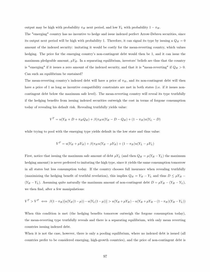
output may be high with probability πH next period, and low YL with probability 1− πH .

The "emerging" country has no incentive to hedge and issue indexed perfect Arrow-Debreu securities, since

its output next period will be high with probability 1. Therefore, it can signal its type by issuing a QH = 0

amount of the indexed security: imitating it would be costly for the mean-reverting country, which values

hedging. The price for the emerging country’s non-contingent debt would then be 1, and it can issue the

maximum pledgeable amount, µYH . In a separating equilibrium, investors’ beliefs are thus that the country

is "emerging" if it issues a zero amount of the indexed security, and that it is "mean-reverting" if QH > 0.

Can such an equilibrium be sustained?

The mean-reverting country’s indexed debt will have a price of πH , and its non-contingent debt will then

have a price of 1 as long as incentive compatibility constraints are met in both states (i.e. if it issues non-

contingent debt below the maximum safe level). The mean-reverting country will reveal its type truthfully

if the hedging benefits from issuing indexed securities outweigh the cost in terms of forgone consumption

today of revealing his default risk. Revealing truthfully yields value:

V T = u(YH +D + πHQH) + β(πHu(YH −D −QH) + (1− πH)u(YL −D)

while trying to pool with the emerging type yields default in the low state and thus value:

V F = u(YH + µYH) + β(πHu(YH − µYH) + (1− πH)u(YL − µYL)

First, notice that issuing the maximum safe amount of debt µYL (and then QH = µ(YH −YL) the maximum

hedging amount) is never preferred to imitating the high type, since it yields the same consumption tomorrow

in all states but less consumption today. If the country chooses full insurance when revealing truthfully

(maximizing the hedging benefit of truthful revelation), this implies QH = YH − YL and thus D ≤ µYH −

(YH − YL). Assuming quite naturally the maximum amount of non-contingent debt D = µYH − (YH − YL),

we then find, after a few manipulations:

V T > V F ⇐⇒ β(1−πH)[u(YH(1−µ))−u(YL(1−µ))] > u(YH +µYH)−u(YH +µYH − (1−πH)(YH −YL))

When this condition is met (the hedging benefits tomorrow outweigh the forgone consumption today),

the mean-reverting type truthfully reveals and there is a separating equilibrium, with only mean reverting

countries issuing indexed debt.

When it is not the case, however, there is only a pooling equilibrium, where no indexed debt is issued (all

countries prefer to be considered emerging, high-growth countries), and the price of non-contingent debt is

97

q + πH(1− q) < 1. If q is sufficiently low, emerging countries may even drop out of the non-contingent debt

market altogether, so that only mean reverting countries issue debt at price πH and in the amount D ≤ µYL.

In other words, if countries are sufficiently impatient, or if the probability of remaining in a high state is

sufficiently high even for mean-reverting countries, the pooling equilibrium is such that no one will issue

indexed debt in "good times", for fear of revealing private information about bad growth prospects. Because

the country has more information than the investor on future growth prospects, issuing zero indexed debt

is a costly (and thus credible) signal that output will remain high, positively influencing the price of non-

contingent debt and thus outweighing the cost of forgone insurance, even for the low type country. While the

country wants hedging, because his knowledge of future income remains uncertain, hedging is costly because

the information revealed may negatively affect the price or the maximum safe limit of non-contingent debt,

so that the low-type country may prefer to hedge via default.

4.2.2. Quantum of solace: indexed debt in bad times

Suppose the country’s current output is now low. It has, again, from the point of view of the investor’s

beliefs, some prior probability q of being an "emerging" economy with only shocks to trend (so that output

remains low next period), and some probability 1− q of being a "mean-reverting" economy (so that output

has a strictly positive probability πH of coming back to the high state).

Then there is some probability that growth will pick up rapidly above its historical mean to revert to trend

("mean-reverting" case), and some risk that it will not and stay at a permanently lower level and persistently

lower growth ("emerging" case). In the two-period case, this means that GDP-indexed bonds are more likely

to pay off to the investor if the current negative shock is transitory and growth is expected to pick up rapidly

and return to trend, rather than if shocks are shocks to trend and growth is likely to remain at a persistently

lower level.

When output is at its lowest level, issuing zero indexed debt can never be a credible signal that output will

be high next period, because if the drop is permanent, it is costless for the country to issue indexed debt (it

expects it never to pay off). Thus there cannot be a separating equilibrium based on the amount of indexed

debt issued. The expected value of the Arrow-Debreu security in a pooling equilibrium is qπH . The pooling

equilibrium will then have QH > 0, because the mean-reverting country wants hedging and has no interest

in mimicking the "persistent-low" country in bad times, while it is costless for the emerging country to issue

indexed debt.

Signalling after default Assume now that a "disaster shock" has occurred, sufficiently negative to

push the country into default. A restructuring occurs, and lenders, who have a claim on the existing face

value of debt, can choose to redeem it in cash, or to obtain GDP-linked instruments which only pay off when

98

growth is above its historical mean. If there has been a shock so negative that default has occurred, the price

of non-contingent debt is no longer determined by market expectations but by negotiations with existing

creditors, as seen in the previous section. The negative signalling impact of indexed debt on the price of

non-contingent debt is thus shut down during restructurings. From the point of view of the restructured

creditor, GDP-indexed bonds can only improve the return over standard bonds, given the low level of output

and the possibility that it may revert to trend.

The country has a choice between remaining in default status, and thus in autarky, or making an offer to

creditors to regain access to capital markets in the next period. The relative value, however, of financial

integration compared to autarky, depends crucially on the nature of the output process, as shown by M.

Aguiar and Gopinath 2006. If output is driven by a stable (non-stochastic) trend - and thus fluctuations

are the result of transitory (possibly persistent) shocks, the welfare benefit of insurance against fluctuations

offered by financial integration is low. On the contrary, if there are stochastic shocks to the trend itself, the

relative value of financial integration compared to autarky, in terms of consumption smoothing, is high. In

other words, reaccessing markets is particularly valuable if output has a stochastic trend and is therefore

more volatile. The intuition is thus that once the default has occurred, GDP-indexed bonds constitute an

optimal renegotiation mechanism: risk-neutral creditors take on the "model mis-specification" risk in lieu of

the country, with only a positive upside possible.

Issuing GDP-indexed bonds during debt restructurings may thus be the only window of opportunity for such

instruments to be available. Because debt is "information-insensitive" as long as there is no default, but

highly information-sensitive upon default, there is no more value to issuing non-contingent debt rather than

equity in order to economize on monitoring (political or material) costs, since those costs must be borne

anyway, due to the default; but the benefits of indexation (risk-sharing and upside potential) remain.

99

Concluding remarks

You see things; and you say "Why?" But I dream things that never were; and

I say "Why not?"The Serpent, George Bernard Shaw

This dissertation intended to characterize the restrictions to sovereign risk-sharing that may account for

the limited prevalence, in practice, of a theoretically optimal financing mechanism, state-contingent sovereign

debt. We assessed the relative magnitude of such limitations as imperfect information (both on the realization

of output (chapter 1) and on the stochastic process driving it (chapter 4)); pricing difficulties (chapter 2);

investor risk-aversion and limited enforcement capacity (chapter 3). The peculiar observation that indexed

debt is mainly observed in the form of debt equity-swaps during restructurings may be rationalized by dilution

concerns for existing creditors, or by uncertainty about the persistence of the output process (chapter 4).

A few key takeaways should be drawn from our work.

• Asymmetric information is in general a powerful argument to prefer debt to equity and reduce infor-

mation acquisition costs (be they material or political). However, it is likely not to be fully binding

for sovereigns, for which proxies closely related to their true ability to pay are much more widely

observable than for private entities. Therefore, imperfect hedging instruments loosely correlated to

a country’s true repayment capacity may be preferable to the crude form of contingency allowed by

costly defaults.

• Imperfect observability of the true ability to pay suggests S-shaped "insurance formulas". However,

the ability of such indexation formulas to reduce default risk and provide financing depends on their

interaction with the GDP process and investor risk-aversion. Formulas including conditions on the

level of GDP appear not to be optimal financing tools, given the volatility in payoffs they involve and

the resulting wide discount at which they would be issued.

• Investor risk-aversion is a major justification for an optimal "sovereign debt-equity mix" rather than

a full transfer of income risk to the lenders. In a general equilibrium framework, while introducing

indexed debt is in general a powerful tool to reduce default risk and support higher levels of debt in

100

equilibrium, investor risk-aversion and its interaction with the output process may affect the optimal

bundle of indexed debt and non-contingent debt issued by the borrower.

• In post-default negotiations, the catastrophic level attained by output and the need to thwart dilution

by "vulture" creditors may justify the use of indexed debt as a complementary restructuring mecha-

nism, in order for existing creditors to capture all of the upside risk from an insolvent (in expectations)

borrower.

Indexed debt, for all of these reasons, is not, as is often argued, the silver bullet to getting rid, once and

for all of sovereign default risk. While it may smooth a country’s ability to pay, asymmetric information

and political economy considerations restrict the upside that creditors can capture in good times, and, by

symmetry, constrain risk sharing in bad times.

However, the significance of these constraints appears limited enough for there to be room for welfare-

improving indexed debt issuance, notably in emerging economies where interest rates are highly counter-

cyclical, and default remains endemic.

Contrary to emerging economies, no unified framework has been provided to think about the potential

use of such instruments for developed countries, and their interaction with the fiscal stance and monetary

policy (with some exceptions, as in Marcus Miller and Lei Zhang 2012 and Brooke et al. 2013). Advanced

economies are currently faced with high debt-to-GDP ratios, and a powerful incentive to hedge against

poor macroeconomic performance, while their monetary policy is often constrained by fixed-exchange rate

arrangements or the zero-lower bound; hence the potential relevance of alternative stabilizers. A key follow-up

alley of research would be to determine whether such instruments could prove useful in this "new normal" of

developed countries, where large burdens of public debt may end up, in the medium-term, requiring efficient

and costless restructuring frameworks. In the same way an initial step backed by developed countries (the

Brady bonds) was paramount in jump-starting a market for emerging sovereign bonds, it is likely that an

initiative by advanced economies to issue indexed bonds would ease their more widespread implementation.

101

Bibliography

Adam, K. and M. Grill (2012). “Optimal Sovereign Default”. In: University of Mannheim Working

Paper 12-16.

Aguiar, M. and M. Amador (2013). Sovereign debt: a review. Tech. rep. National Bureau of Economic

Research.

Aguiar, M. and G. Gopinath (2006). “Defaultable Debt, Interest Rates and the Current Account”.

In: Journal of International Economics 69.1, pp. 64–83.

— (2007). “Emerging Market Business Cycles: The Cycle Is the Trend”. In: Journal of Political

Economy 115.1, pp. 69–102.

Aguiar, Mark et al. (2014). “Sovereign debt booms in monetary unions”. In: The American Economic

Review 104.5, pp. 101–106.

Alfaro, L. and F. Kanczuk (2005). “Sovereign debt as a contingent claim: a quantitative approach”.

In: Journal of International Economics 65.2, pp. 297–314.

Arellano, C. (2008). “Default Risk and Income Fluctuations in Emerging Economies”. In: American

Economic Review 98.3, pp. 690–712.

Arellano, C. and A. Ramanarayanan (2012). “Default and the maturity structure in sovereign bonds”.

In: Journal of Political Economy 120.2, pp. 187–232.

Athanasoulis, S., R. Shiller, and E. van Wincoop (1999). “Macro Markets and Financial Security”.

In: Economic Policy Review 5.1, pp. 21–40.

Barr, D., O. Bush, and A. Pienkowski (2014). “GDP-linked bonds and sovereign default”. In: Bank

of England Working Paper 484.

Barro, R. (1995). “Optimal debt management”. In: NBER Working Paper 5327.

102

Benjamin, David and Mark LJ Wright (2009). “Recovery before redemption: A theory of delays in

sovereign debt renegotiations”. In: Available at SSRN 1392539.

Bersem, Mario R. C. (2012). Incentive-Compatible Sovereign Debt. WorkingPaper. SSRN: Social

Science Research Network.

Blanchard, O., P. Mauro, and J. Acalin (2016). “The Case for Growth-Indexed Bonds in Advanced

Economies Today”. In: Peterson Institute for International Economics Policy Briefs.

Bolton, Patrick and Olivier Jeanne (2009). “Structuring and restructuring sovereign debt: The role

of seniority”. In: The Review of Economic Studies 76.3, pp. 879–902.

Borensztein, E., M. Chamon, et al. (2004). “Sovereign Debt Structure for Crisis Prevention”. In:

International Monetary Fund Policy Paper.

Borensztein, E. and P. Mauro (2002). “Reviving the case for GDP-indexed bonds”. In: IMF Policy

discussion paper 02/10.

Borri, Nicola and Adrien Verdelhan (2011). “Sovereign risk premia”. In: AFA 2010 Atlanta Meetings

Paper.

Brooke, M. et al. (2013). “Sovereign default and state-contingent debt”. In: Bank of England Finan-

cial Stability Paper 27.

Bulow, J. and K. Rogoff (1989). “Sovereign Debt: Is to Forgive to Forget?” In: The American

Economic Review 79.1, pp. 43–50.

Caballero, Ricardo J and Stavros Panageas (2004). Contingent reserves management: an applied

framework. Tech. rep. National Bureau of Economic Research.

Callen, M., J. Imbs, and P. Mauro (2015). “Pooling risk among countries”. In: Journal of Interna-

tional Economics 96.1, pp. 88–99.

Catão, Luis AV, Ana Fostel, and Sandeep Kapur (2009). “Persistent gaps and default traps”. In:

Journal of Development Economics 89.2, pp. 271–284.

Chamon, Marcos, Alejo Costa, and Luca A Ricci (2008). “Is there a novelty premium on new financial

instruments? The Argentine experience with GDP-indexed warrants”. In: IMF Working Papers,

pp. 1–40.

Christiano, Lawrence J and Martin Eichenbaum (1990). “Unit roots in real GNP: Do we know,

and do we care?” In: Carnegie-Rochester Conference Series on Public Policy. Vol. 32. Elsevier,

pp. 7–61.

103

Cochrane, J. (2001). Asset pricing. Princeton University Press.

Cochrane, J. H. and M. Piazzesi (2009). “Decomposing the yield curve”. In: AFA 2010 Atlanta

Meetings Paper.

Cochrane, John H (1991). “[Pitfalls and Opportunities: What Macroeconomists Should Know about

Unit Roots]: Comment”. In: NBER macroeconomics annual 6, pp. 201–210.

Cohen, Daniel and Sebastien Villemot (2015). “Endogenous debt crises”. In: Journal of International

Money and Finance 51, pp. 337–369.

Cole, Harold L and Timothy J Kehoe (2000). “Self-fulfilling debt crises”. In: The Review of Economic

Studies 67.1, pp. 91–116.

Cuadra, Gabriel and Horacio Sapriza (2008). “Sovereign default, interest rates and political uncer-

tainty in emerging markets”. In: Journal of International Economics 76.1, pp. 78–88.

Drelichman, M. and H-J. Voth (2015). Lending to the borrower from hell: Debt, Taxes, and Default

in the Age of Philip II.

Drelichman, Mauricio and Hans-Joachim Voth (2013). “Contingent Sovereign Debt Contracts: The

Historical Perspective”. In: DICE Report 11.3, p. 28.

Durdu, Ceyhun Bora (2009). “Quantitative implications of indexed bonds in small open economies”.

In: Journal of Economic Dynamics and control 33.4, pp. 883–902.

Eaton, J. and M. Gersovitz (1981). “Debt with Potential Repudiation: Theoretical and Empirical

Analysis”. In: The Review of Economic Studies 48.2, pp. 289–309.

Faria, A. (2007). Growth-Indexed Bonds in Emerging Markets: A Quantitative Approach. Mimeo.

Fernandez, R. and R. Rosenthal (1990). “Strategic models of sovereign-debt renegotiations”. In: The

Review of Economic Studies 57.3, pp. 331–349.

Gale, D. and M. Hellwig (1985). “Incentive-compatible debt contracts: the one-period problem”. In:

Review of Economic Studies 52, pp. 647–663.

Gerber, Hans U, Elias SW Shiu, et al. (1994). “Option pricing by Esscher transforms”. In: Transac-

tions of the Society of Actuaries 46.99, p. 140.

Griffith-Jones, S. and D. Hertova (2013). “Growth-linked bonds”. In: CESifo DICE Report 3.

Griffith-Jones, S. and K. Sharma (2006). “GDP-indexed bonds: making it happen”. In: UN/DESA

Working Paper 21.

104

Grossman, H. I. and J.B. Van Huyck (1988). “Sovereign Debt as a Contingent Claim: Excusable

Default, Repudiation, and Reputation”. In: American Economic Review 78, pp. 1088–1097.

Hatchondo, J. C. and L. Martinez (2012). “On the Benefits of GDP-Indexed Government Debt:

Lessons from a Model of Sovereign Defaults”. In: Economic Quarterly 98.2, pp. 139–157.

Kehoe, Timothy J and David K Levine (1993). “Debt-constrained asset markets”. In: The Review

of Economic Studies 60.4, pp. 865–888.

Krueger, Dirk and Harald Uhlig (2006). “Competitive risk sharing contracts with one-sided com-

mitment”. In: Journal of Monetary Economics 53.7, pp. 1661–1691.

Krugman, P. (1988). “Financing vs. Forgiving a Debt Overhang”. In: Journal of Development Eco-

nomics 29, pp. 253–68.

— (1996). “A country is not a company”. In: Harvard Business Review.

Kruse, S., M. Meitner, and M. Schröder (2005). “On the Pricing of GDP- Linked Financial Products”.

In: Applied Financial Economics 15.16, pp. 1125–1133.

Levasseur, Émile (1854). Recherches historiques sur le système de Law. Guillaumin et cie.

Lizarazo, Sandra Valentina (2013). “Default risk and risk averse international investors”. In: Journal

of International Economics 89.2, pp. 317–330.

Mauro, P. and M. Chamon (2006). “Pricing Growth-Indexed Bonds”. In: Journal of Banking and

Finance 30.12, pp. 3349–3366.

Mendoza, G. and V. Yue (2012). “A General Equilibrium Model of Sovereign Default and Business”.

In: Quarterly Journal of Economics 127.2, pp. 889–946.

Miller, M. and L. Zhang (2013). “Avoiding costly default with state-contingent contracts: issues of

market power and moral hazard”. In: Bank of England Working Papers.

Miller, Marcus and Lei Zhang (2012). “Beyond austerity: an SPV to save the Eurozone?” In: Inter-

national Economic Association.

Myiajima, K. (2006). “How to Evaluate GDP-Linked Warrants: Price and Repayment Capacity”.

In: IMF Working Paper 85.

Obstfeld, M., K. Rogoff, and S. Wren-Lewis (1996). Foundations of international macroeconomics.

Vol. 30. MIT press Cambridge, MA.

Park, Stephen Kim and Tim R Samples (2016). “Towards Sovereign Equity”. In: Stanford Journal

of Law, Business, and Finance.

105

Petrova, I., M. Papaioannou, and M. Bellas (2010). “Determinants of emerging market sovereign

bond spreads: fundamentals vs financial stress”. In: International Monetary Fund Working Paper

10-281.

Pina, G. (2015). GDP-Indexed Sovereign Debt with Risk Averse Lenders. Link.

Presno, I. and D. Pouzo (2012). “Sovereign Default Risk and Uncertainty Premia”. In: 2012 Meeting

Papers. 608. Society for Economic Dynamics.

Rochet, Jean-Charles (2006). “Optimal sovereign debt: an analytical approach”. In: IADB Working

Papers Series.

Ross, Stephen A (1977). “The determination of financial structure: the incentive-signalling ap-

proach”. In: The Bell journal of economics, pp. 23–40.

Ruban, Oleg A., Luiz Vitiello, and Ser-Huang Poon (2014). Pricing GDP Linked Securities.

Sachs, Jeffrey and Daniel Cohen (1982). “LDC Borrowing with Default Risk”. In: NBER Working

Paper Series, p. 925.

Sandleris, G., H. Saprizza, and G. Taddei (2011). “Indexed Sovereign Debt: An Applied Framework”.

In: The Colegio Alberto Notebooks Working Paper 104.

Sandleris, G. and M. Wright (2013). “GDP-indexed bonds: A tool to reduce macroeconomic risk?”

In: The future of sovereign borrowing in Europe.

Schinckus, C. (2013). “How to Value GDP-Linked Collar Bonds? An Introductory Perspective”. In:

Theoretical Economics Letters 3, pp. 152–155.

Shiller, R. (1993). Macro markets. Creating institutions for managing society’s largest economic

risks. Oxford University Press.

Sumner, Scott (2006). “Let a Thousand Models Bloom: The Advantages of Making the FOMC a

Truly’Open Market’”. In: Contributions in Macroeconomics 6.1, pp. 1–27.

Tamayo, C. (2015). “Investor protection and optimal contracts under risk aversion and costly state

verification”. In: Economic Theory 59.3, pp. 547–577.

Tauchen, George and Robert Hussey (1991). “Quadrature-based methods for obtaining approxi-

mate solutions to nonlinear asset pricing models”. In: Econometrica: Journal of the Econometric

Society, pp. 371–396.

Townsend, Robert M (1979). “Optimal contracts and competitive markets with costly state verifi-

cation”. In: Journal of Economic theory 21.2, pp. 265–293.

106

Velde, François R (2007). “John Law’s System”. In: The American economic review 97.2, pp. 276–

279.

Von Weizsäcker, Jakob, Jacques Delpla, et al. (2010). The blue bond proposal. Bruegel.

Williamson, John (2005). Curbing the boom-bust cycle: stabilizing capital flows to emerging markets.

Peterson Institute.

Yue, Vivian Z (2010). “Sovereign default and debt renegotiation”. In: Journal of international Eco-

nomics 80.2, pp. 176–187.

107

Appendix A

Proofs

A.1. Proof of lemma 1.2.1

Proof. Notice first that, if QJ = 0, the covariance term equals

Cov(1J , u′(C2)) = πHu

′(YH −D)(ψH − η) + πLu′(YL −D)(ψL − η)

It is not zero, except if ψH = ψL (i.e. except if the signal is not informative). This is true because, if QJ = 0,

D > 0 (given that output is zero in t0 and limc→0 u′(c) = −∞), so 0 < u′(YH −D) ≤ u′(YL −D) because

u′′ < 0, and since ψL ≤ ψH , Cov(1J , u′(C2)) ≤ u′(YL −D)(ψL − η) ≤ 0, with the inequality holding with

equality only if ψL = η = ψH . This implies that the optimum quantity of Arrow-Debreu security issued

cannot be zero, as long as the signal is correlated with the good state (ψH > ψL).

We can show, furthermore, that the optimal quantity is positive. By contradiction, assume it is negative

QJ < 0. Then, by concavity of the utility function:

E(1J)E(u′(C)) = η [πH [ψHu′(YH −D −QJ) + (1− ψH)u′(YH −D)] + πL[ψLu

′(YL −D −QJ) + (1− ψL)u′(YL −D)]]

ηE(u′(C)) > η(πHu′(YH −D −QJ) + πLu

′(YL −D −QJ))

But, on the other hand, because ψH > ψL, η > ψL, and thus, again using concavity, (η − ψL)u′(YL −D −

QJ)) ≥ (η − ψL)u′(YH −D −QJ)). Then:

η(πHu′(YH−D−QJ)+πLu

′(YL−D−QJ))−E(1Ju′(C2)) = πH(η−ψH)u′(YH−D−QJ)+πL(η−ψL)u′(YL−D−QJ))

η(πHu′(YH−D−QJ)+πLu

′(YL−D−QJ))−E(1Ju′(C2)) ≥ πH(η−ψH)u′(YH−D−QJ)+πL(η−ψL)u′(YH−D−QJ))

108

≥ u′(YH −D −QJ)(η(πH + πL)− πHψH − πLψL) ≥ u′(YH −D −QJ)(η − η) = 0

so that ηE(u′(C)) > η(πHu′(YH − D − QJ) + πLu

′(YL − D − QJ)) ≥ E(1Ju′(C2)) and we would have

Cov(1J , u′(C2)) = E(1Ju

′(C2))− ηE(u′(C)) < 0, which is the contradiction.

A.2. Proof of lemma 1.2.2

Proof. To see this, it is sufficient to prove that issuing the full amount of the difference in income between

states brings "too high" a covariance between the signal and marginal utility. Assume that the government

does issue QJ = Q∗H = YH − YL. Then:

E(1J)E(u′(C)) = η [πH [ψHu′(YL −D) + (1− ψH)u′(YH −D)] + πL[ψLu

′(YL −D − (YH − YL)) + (1− ψL)u′(YL −D)]]

By concavity of the utility function, and because the signal is not fully informative (ψH < 1 and ψL > 0):

ηE(u′(C)) ≤ η(πHu′(YL −D) + πL(ψLu

′(YL −D − (YH − YL)) + (1− ψL)u′(YL −D))

But, on the other hand, because the signal is not fully informative (ψH < 1 and ψL > 0), and, again, using

concavity:

E(1Ju′(C2))− η(πHu

′(YL −D) + πL(ψLu′(YL −D − (YH − YL)) + (1− ψL)u′(YL −D))

= [πH(ψH − η)− ηπL(1− ψL)]u′(YL −D) + πLψL(1− η)u′(YL −D − (YH − YL)))

= [πHψH + ηπLψL − η]u′(YL −D) + πLψL(1− η)u′(YL −D − (YH − YL)))

= [(η − 1)πLψL]u′(YL −D)πLψL(1− η)u′(YL −D − (YH − YL)))

= [(1− η)πLψL](u′(YL −D − (YH − YL))− u′(YL −D)) > 0

so that ηE(u′(C)) ≤ ηη(πHu′(YL−D)+πL(ψLu

′(YL−D−(YH−YL))+(1−ψL)u′(YL−D)) < E(1J , u′(C2))

and we would have Cov(1J , u′(C2)) = E(1Ju

′(C2))− ηE(u′(C)) > 0, which is the contradiction.

109

A.3. Proof of proposition 1.2.4

Proof. The value of the unsafe case is, as in case 1:

V U = maxµYL≤DU≤µYH

u(DUπH1 + r

) + β(πHu(YH −DU ) + (1− πH)u(YL(1− µ)))

while the value of the safe, contingent case is:

V SJ = maxDS ,QJ s.t. DS+QJ≤µYL

u(DS + ηQJ

1 + r)

+β(πH(ψHu(YH −DS−QJ)+(1−ψH)u(YH −DS))+(1−πH)(ψLu(YL−DS−QJ)+(1−ψL)u(YL−DS)))

If the signal is not informative at all (ψH = ψL = ψ so that ∆ψ = 0), then:

V SJ(∆ψ = 0) = maxDS ,QJ s.t. DS+QJ≤µYL

u(DS + ψQJ

1 + r)

+β(πH(ψu(YH −DS −QJ) + (1− ψ)u(YH −DS)) + (1− πH)(ψu(YL −DS −QJ) + (1− ψ)u(YL −DS)))

In such a case, the optimal amount of indexed debt is zero (as seen in the non-default case), implying

that V SJ = V S < V U . On the contrary, when the signal is perfectly informative ψH = 1ψL = 0 so that

∆ψ = 1, we are under case-2 contingency (complete markets), and, as proven before, a strictly positive

amount of contingent debt is preferred to the unsafe case (V SJ = V H > V U ). Since V U does not depend

on ∆ψ, and V SJ is clearly increasing in the signal’s informativeness, and given V U − V SJ(∆ψ = 0) > 0,

V U − V SJ(∆ψ = 0) < 0, there exists a critical "informativeness" threshold (∆ψ = ψH − ψL = ∆) such that

for ∆ψ = ψH −ψL ≥ ∆, the safe contingent option is preferred to the unsafe contingent case, and conversely

for ψH − ψL ≤ ∆.

A.4. Proof of lemma 1.2.3

Proof. We claim the alternative facing the country is between (a) the unsafe, pure non-contingent debt

strategy with default in the low state; or (b) a safe debt strategy including a mix of debt and the J-security

such that one never defaults. To see this, notice first that if the safe, non-contingent strategy was preferred to

the unsafe case under case 1 (V S > V U ), then (b) is also preferred to (a), since (b) may improve consumption

smoothing in period 2 over the safe non-contingent case via the J-security, while still providing the same

maximal amount of financing (safe, non-contingent is a subset of (b)).

On the contrary, consider the case where unsafe debt was preferred to safe, non-contingent debt (V S ≤ V U ).

110

Suppose the country chooses an unsafe mix of debt (D) and a positive amount of the J-security QJ > 0 (we

rule out a negative amount of the security by the same arguments as in the case without default).

Default occurs in some states, which can only be:

• all of the bad states (if D +QJ > µYL and D +QJ ≤ µYH)

• all of the J-states (if D +QJ > µYH and D ≤ µYL)

• or all cases except the high, non-J state (if D +QJ > µYH and µYL < D ≤ µYH)

We now show that such a mix is always dominated by pure unsafe non-contingent debt. If default occurs

in bad cases, there is no improvement of having J-debt over pure D-debt in terms of consumption volatility,

since unsafe debt payoffs are perfectly correlated with marginal utility of consumption, and PJ = πHψH1+r <

PD = πH1+r , so J-debt offers no improvement. Then, if QJ > 0 and default occurs in all cases except high,

non-J, the price of J-debt is PJ = 0, and there is a contradiction because issuing QJ = 0 is preferred. If

QJ > 0 and default occurs in all J-states, this implies that D ≤ µYL, PD = 1− η, and the price of J-debt is

again PJ = 0; so no unsafe debt will be issued, leading again to a contradiction.

A.5. Proof of proposition 1.3.1

Proof. Formally, assume u′(y) < ζ, and suppose ∃y > y such that β(y) = 0. We have, by strict concavity of

the utility function: u′(y − β(y)) = u′(y) < u′(y) < ζ. But note that β(y) = 0 implies µ2(y) = 0 (making

the natural assumption y > 0), so that ζ − u′(y) = −µ1(y)f(y) ≤ 0, which is a contradiction. Conversely, assume

u′(y) > ζ. By continuity of u′, ∃y > y such that u′(y) > ζ. This implies µ2(y) − µ1(y) < 0. This in turns

implies µ1(y) > 0 and thus β(y) = 0.

A.6. Proof of proposition 1.3.2

Proof. Suppose, without loss of generality, that there is an optimal contract where A is the disjoint union

of two intervals, (y, x) and (s1, s2). The country’s utility in that case is:

U =

∫ x

y

u(y−β(y) + b)dF (y) +

∫ s1

x

u(y− R+B)dF (y) +

∫ s2

s1

u(y−β(y) + b)dF (y) +

∫ y

s2

u(y− R+B)dF (y)

and the investor’s payoff is:

V =

∫ x

y

β(y)dF (y) + R(F (s1)− F (x)) +

∫ s2

s1

β(y)dF (y) + R(1− F (s2)

111

We can then, because R ≥ β(y) + (B − b), find β(y) + B − b ≤ RZ < R to construct a new contract

Z, defined by a new auditing region corresponding solely to the lower part of the former auditing region

AZ ={y|y ∈ (y, x)

}and x, RZ , β(y) such that it meets the investor’s participation constraint:

V Z =

∫ x

y

β(y)dF (y) + RZ(1− F (x) = V

This contract thus satisfies the investor’s individual rationality constraint.

Moreover, since the initial contract was incentive-compatible, the new contract also respects the incentive

compatibility constraint in the auditing region AZ . In the non-auditing region, because the old contract was

such that R ≤ λy +B ∀y ∈ A, and in particular R ≤ λx+B, the new contract is also incentive-compatible:

RZ < R ≤ λx+B ≤ λy +B ∀y ∈ A, and RZ ≥ β(y).

It remains to show that the new contract improves the country’s welfare (UZ > U). We have:

UZ =

∫ x

y

u(y − β(y) + b)dF (y) +

∫ y

x

u(y − RZ +B)dF (y)

UZ > U follows from the concavity of the utility function:

UZ − U =

∫ s1

x

[u(y − RZ +B)− u(y − R+B)]dF (y) +

∫ s2

s1

[u(y − RZ +B)− u(y − β(y) + b)]dF (y)

+

∫ y

s2

[u(y − RZ +B)− u(y − R+B)]dF (y)

UZ − U >

∫ s1

x

[u(y − RZ +B)− u(y − R+B)]dF (y) +

∫ s2

s1

[u(y − RZ +B)− u(y − β(y) +B)]dF (y)

+

∫ y

s2

[u(y − RZ +B)− u(y − R+B)]dF (y)

UZ − U > 0

because of the concavity of the utility function, because the new consumption pattern is strictly higher (via

the increase in political benefit from b to B over some range) than (loosely speaking) a mean-preserving

contraction of the former consumption pattern. In other words, transferring lower (indexed) repayments

towards lower states of the world and higher (fixed) repayments towards higher states of the world, keeping

expected total payments to the investor constant, is a Pareto-improving change, since it leaves the investor

as well-off and the country strictly better-off. Thus the auditing region is a lower interval.

112

A.7. Proof of proposition 1.3.3

Proof. To show this, assume R < λy∗ + B. This implies that the willingness-to-pay constraint was not

binding in unaudited states (otherwise R− β(y∗) = R− λy∗ − b < B − b and the IC constraint is violated).

Then µ2(y∗) = µ3(y∗) = µ4 = µ5 = 0. This means, however:

ζ(R− β(y∗)) = u(y∗ − β(y∗) + b)− u(y∗ − R+B)

Then there are two cases. First suppose µ6(y∗) > 0, in which case, β(y∗)− b = R − B. Then the only way

the former equality can hold (since the left hand side is strictly positive if ζ > 0 and the right hand side is

zero) is if ζ = 0. However, this entails:

−f(y∗)u′(y∗ − β(y∗) + b) = µ6(y∗)− µ1(y∗)

and since µ6(y∗) > 0, this requires µ1(y∗) > 0, so β(y∗) = 0, and the contract is a two-step contract that

specifies zero repayment in all audited states, and R = B − b in unaudited states. Therefore, if the contract

is not the two-step contract, it implies β(y∗)− b < R−B and µ6(y∗) = 0.

A.8. Proof of proposition 1.4.1

Proof. We want to show that repayments in unaudited states are non-decreasing in yOBS . Supposed that

there exists an optimal contract with a set T of unaudited states where repayments are decreasing strictly

in yOBS . Over this region (loosely speaking), the expected utility of the borrower for is:

E(UT ) =

∫T

∫T

u(y − β(yOBS) +B)dH(yOBS |y)dF (y)

Because the signal is yOBS = y + ε, we have (with φ the density of the normal distribution):

E(UT ) =

∫T

∫T

u(y − β(yOBS) +B)φ(yOBS − y)dF (y)

Define R such that

R =

∫T

∫T

β(yOBS)φ(yOBS − y)dF (y)

(the "certainty" equivalent of β(yOBS) over set T ). Repaying such an amount in any state belonging

to T leaves the investor at least as well off ex ante. We want to show that this new repayment schedule,

yielding E(URT ), strictly improves the borrower’s welfare ex ante relative to the strictly decreasing repayment

113

schedule, and thus that the latter cannot be an optimal contract. The concavity of u, together with the

positive correlation of yOBS with y, imply that a strictly decreasing schedule β(yOBS) = β(y + ε) makes

repayments positively correlated with the marginal utility of consumption, thus providing lower welfare than

constant repayments, for a given consumption mean over the region:

E(URT )−E(UT ) =

∫ ∫T

[u(y −R+B)− u(y − β(y + ε) +B)]φ(ε)dF (y) > 0

A.9. Proof of proposition 1.4.2

Proof. Consumption in non-audited states is (omitting the government’s political benefit) y− κ(y+ ε). The

optimal indexation formula minimizes the variance of consumption in non-audited states, which is given by:

Var(C|A) = (1− κ)2Var(Y |A) + κ2Var(ε|A)

Var(C|A) = (1− κ)2Var(Y |ε < 0) + κ2Var(ε|ε < 0)

and the first-order condition to this minimization problem implies immediately that κ is decreasing in

Var(ε).

A.10. Proof of lemma 3.2.3

Proof. One result (Prop.2 of Arellano 2008) states that, if the default set is non-empty for some level of non-

contingent debt, then no contract exists such that the economy experiences capital inflows (in our notations,

if D(bt) 6= ∅, then @qB(st+1, bt+1, Yt)bt+1 − bt + qS(st+1, bt+1, Yt)st+1 − stκ(Yt) > 0). This result still holds

in the presence of indexed debt, with a similar proof. Assume the default set is non-empty, ∃y such that

V D(Y ) > V R(s, b, Y ). Suppose there exists a capital inflow contract qBb′ + qSs′ − b − sκ(Y ) > 0. Then,

taking the contract and defaulting next period would be preferred to default nd thus:

V D(Y ) = u(Y ) + βE(V D(Y ′)) ≤ u(Y ) + βE(V D(Y ′)) ≤ u(Y + qBb′ + qSs

′ − b− sκ(Y )) + βE(V D(Y ′))

V D(Y ) ≤ u(Y + qBb′ + qSs

′ − b− sκ(Y )) + βE(V G(b′, s′, Y ′)) ≤ V R(s, b, Y )

which is the contradiction, so that net capital inflows are not possible if default sets are non empty.

114

A.11. Proof of proposition 3.2.4

Proof. For i.i.d. income shocks, we have:

V R(s, b, Y )− V D(Y ) = u(Y + qBb′∗ + qSs

′∗ − b− sκ(Y ))− u(Y ) + β(E(V G(s′∗, b′∗, Y ′)−E(V D(Y ′)))

By the envelope theorem, we have:

dV R(s, b, Y )− V D(Y )

dY= V Ry (s, b, Y )− V Dy (Y ) = (1− sκ′(Y ))u′(Y + qBb

′∗ + qSs′∗ − b− sκ(Y ))− u′(Y )

Now, the result that if the default set is non-empty, only capital outflows contracts are available, jointly with

utility concavity, implies that u′(Y + qBb′∗ + qSs

′∗ − b − sκ(Y )) > u′(Y ): in the absence of indexed debt,dV R(s,b,Y )−V D(Y )

dY ≥ 0 and default sets are shrinking in income. However, here the first term is scaled down

by 1 − sκ′(Y ). There is a "race between utility concavity and debt indexation" that determines when the

Arellano result still holds.

dV R(s, b, Y )− V D(Y )

dY≥ 0 ⇐⇒ sκ′(Y )) ≤ u′(Y + qBb

′∗ + qSs′∗ − b− sκ(Y ))− u′(Y )

u′(Y + qBb′∗ + qSs′∗ − b− sκ(Y ))

For small enough net capital outflows, a first-order Taylor approximation of u′ yields:

dV R(s, b, Y )− V D(Y )

dY≥ 0 ⇐⇒ sκ′(Y )) ≤ u′′(Y )(qBb

′∗ + qSs′∗ − b− sκ(Y ))

u′(Y )

In words, for a given shape of the indexation formula κ′(Y ), and a given "degree of concavity" (a curvature

of the utility function) there exists an amount S such that default sets are shrinking in income if and only

if S-debt issued is below that amount.

A.12. Proof of lemma 3.2.5

Proof. When the default set is empty,

Cov(1− δ′, κ(Y ′)) = Cov(1− δ′, v′L(c′L)) = 0

and

Cov((1− δ′)κ(Y ′), v′L(c′L)) = Cov(κ(Y ′), v′L(c′L))

115

Therefore, in that case:

qB(θ′S , θ′B , Y )− qS(θ′S , θ

′B , Y ) = −βL

Cov(κ(Y ′), v′L(c′L))

v′L(cL)

However, we have, in the absence of default, that lender’s wealth next period is positively correlated with

the economy’s output. Let Y ′1 > Y ′2 , then, assuming (quite naturally) a non-decreasing indexation process

(κ′(Y ) ≥ 0) implies:

[W ′|Y ′1 ] = θ′S + κ(Y ′1)θ′S) + θ′A ≥ θ′S + κ(Y ′2)θ′S) + θ′A

[c′L|Y ′1 ] ≥ [c′L|Y ′2 ]

and by concavity of utility

[v′L(c′L)|Y ′1 ] ≤ [v′L(c′L)|Y ′2 ]

so that Cov(κ(Y ′), v′L(c′L)) < 0, and therefore qB(θ′S , θ′B , Y ) ≥ qS(θ′S , θ

′B , Y ).

A.13. Proof of proposition 4.1.2

Proof. The value for diluted creditors can be expressed as:

ZR,DIL(L) = D − L+1

R[L

ε+ Lλµ

∫ (εQNEW+LQOLD)γ

y

ydF (y|y1) +

∫ y

(εQNEW+LQOLD)γ

LQOLDdF (y|y1)]

= γy1 +1

R[L

Bλµ

∫ (εQNEW+LQOLD)γ

y

ydF (y|y1)−∫ y

(εQNEW+LQOLD)γ

L(QNEW −QOLD)dF (y|y1)

+BR−∫ y

(εQNEW+LQOLD)γ

εQOLDdF (y|y1)− λµ∫ (εQNEW+LQOLD)

γ

y

ydF (y|y1)]

= γy1 +1

R[BR− ε

ε+ Lλµ

∫ (εQNEW+LQOLD)γ

y

ydF (y|y1)−∫ y

(εQNEW+LQOLD)γ

εQNEW dF (y|y1)

−∫ y

(εQNEW+LQOLD)γ

L(QNEW −QOLD)dF (y|y1)]

= γy1 +1

R[BR− εR−

∫ y

(εQNEW+LQOLD)γ

L(QNEW −QOLD)dF (y|y1)]

= γy1 + L− 1

R[

∫ y

(εQNEW+LQOLD)γ

L(QNEW −QOLD)dF (y|y1)]

116

= D − 1

R[

∫ y

(εQNEW+LQOLD)γ

L(QNEW −QOLD)dF (y|y1)]

117

Appendix B

Some preliminary thoughts on

endogenous output

I outline below some preliminary issues (to be explored in future work) related to endogeneizing output in

a general equilibrium model with both indexed debt and non-contingent debt.

Moral hazard issues with indexed debt An additional restriction on the benefits of sovereign debt

when output is endogenous comes from moral hazard issues. Indeed, assume that the government can affect

production. More specifically, it can choose to exert a high level of "effort", e = eH , in which case the

respective probabilities of each of the states occurring are pH and 1− pH ; or a low level of effort, normalized

to zero, where the respective probabilities of each of the states occurring are qH and 1− qH with qH < pH .

Effort is assumed to have utility cost c such that

β (E(U(C2)|e = eH)−E(U(C2)|e = 0)) > c

(the first-best level of effort without access to contingent debt is trivially e). Under indexed debt, however,

and with full insurance, the government has no incentive to exert the high level of effort and increase the

likelihood of the high state, since consumption will be equal in both states of the world. This moral hazard

issue may be less pronounced in richer versions of the model, but it will still play a role in the design of

indexed debt contracts and their ability to reduce macroeconomic volatility.

Risk of multiple equilibria Under endogenous output, if investment is itself financed by indexed debt,

multiple equilibria may emerge for given fundamentals. We can model this very simply by assuming that

indexed debt pays a share of income in period 2, which is itself entirely deterministic and depends on period

118

1 investment, financed by debt. Because in one equilibrium, high levels of indexed debt mean an ability to

finance high level of investment, thus high expected output, thus higher price for indexed debt, supporting

the high issuance decision. But there may be another equilibrium with zero debt, zero investment, zero

expected output, and zero price for indexed debt. Then if only indexed debt is possible, and it is the only

source of financing available for investment, an equilibrium with the first-best level of investment is possible

(at f ′(KFB) = 1 + r and pI = κf(KFB)1+r ), but so is an equilibrium with zero investment and zero production

in period 2. It is likely that introducing non-contingent debt would rule out such bad equilibria, by allowing

the country to issue debt whose repayment is unconditional on the level of income attained, and thus priced

simply at its "default risk" level.

Interaction with monetary policies Another key issue, once we introduce the case of endogenous

output, would be the interaction of debt management with other policies affecting output growth. In par-

ticular, in advanced economies, "lean-against-the-wind" monetary policy already performs the function that

we deemed useful for indexed debt in emerging economies, namely introducing pro-cyclical interest rates.

The one instance in which indexed debt could be relevant is therefore when interest rates are constrained

by the zero lower bound for monetary policy, with negative indexed sovereign rates pushing the boundary

below zero. However, this may raise the question of whether sovereign debt yields would still be considered

the "risk-free" rate by financial markets.

Interaction with tax policies Tax policies would also need to be taken into account, once the dynamics

of output are endogenous. In particular, while higher taxes are welcome by non-contingent bondholders (as

long as they do not push output under the default boundary), because they raise additional resources

to pay off debt, they would have an ambiguous effect on indexed debt holders. On the one hand, the

"resource-raising" effect is positive (but this is not relevant away from the default threshold); but on the

other hand, higher taxes may stifle output growth and reduce the interest rate paid on sovereign indexed

debt. Therefore, inter-creditor conflicts may emerge between non-contingent and indexed bondholders over

the optimal taxation schedule.

In particular, if repayment is determined by the country’s ability to pay only (when tax revenues τy(τ) are

larger than repayment obligation B+Sκ(y(τ)), the tax rate that maximizes the expected payoff on indexed

debt (τ = arg maxκ(y(τ))P (τy(τ) > B + Sκ(y(τ))) may then be different from the tax rate maximizing

expected repayment probability for non-contingent debt (τ = arg maxP (τy(τ) > B+Sκ(y(τ))). A paradox

of austerity could arise, where "equity owners" would demand less fiscal consolidation, while non-contingent

debt owners require more: the former have an interest in growth being high; the latter in fiscal resources

being sufficient to cover non-contingent debt.

119

Appendix C

Indexation calibration

120

(a) Formula 1 (b) Formula 2

(c) Formula 3 (d) Formula 4

(e) Formula 5

Figure C.1: Process 2: persistent transitory shocks

121

(a) Formula 1 (b) Formula 2

(c) Formula 3 (d) Formula 4

(e) Formula 5

Figure C.2: Process 3: stochastic trend

122

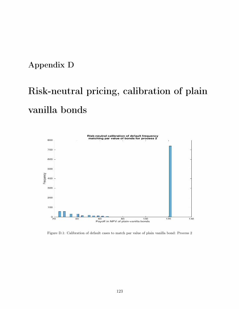
Appendix D

Risk-neutral pricing, calibration of plain

vanilla bonds

Figure D.1: Calibration of default cases to match par value of plain vanilla bond: Process 2

123

Figure D.2: Calibration of default cases to match par value of plain vanilla bond: Process 3

124

Appendix E

Risk-neutral pricing, indexed bonds with

default risk

125

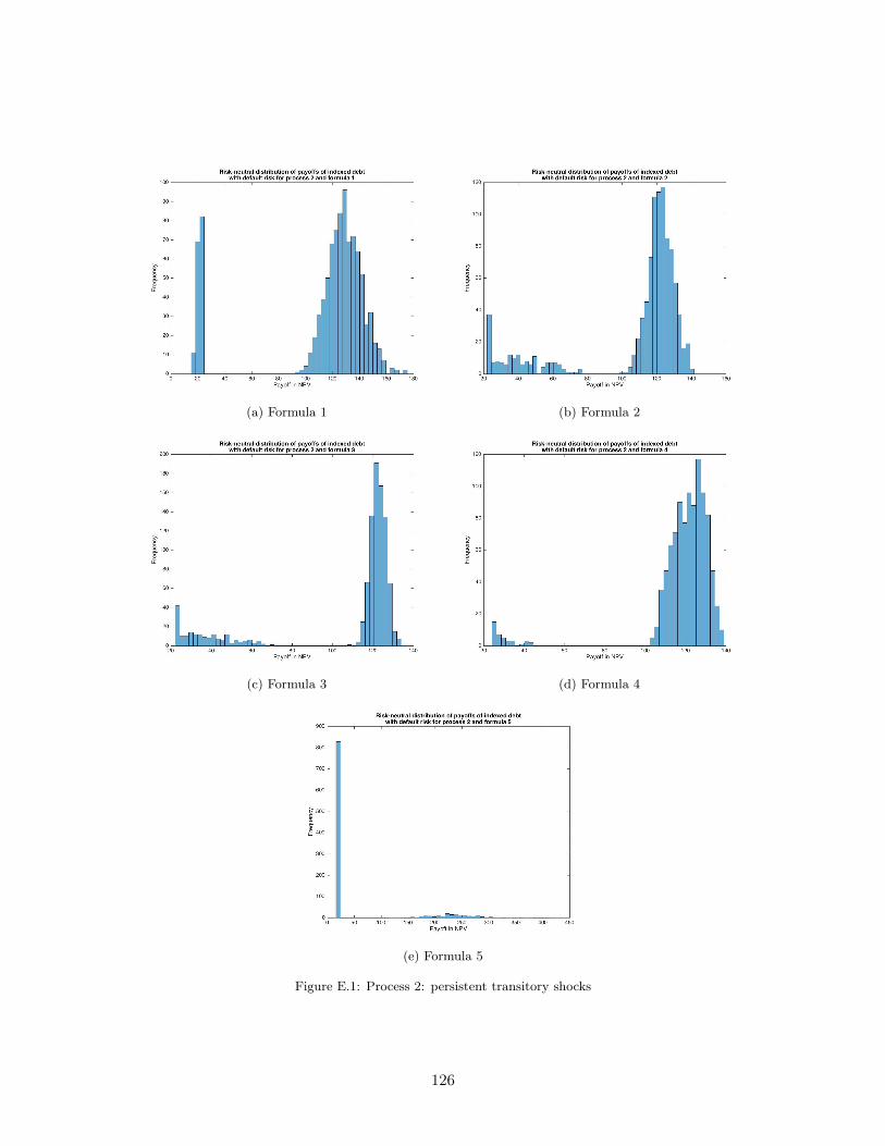
(a) Formula 1 (b) Formula 2

(c) Formula 3 (d) Formula 4

(e) Formula 5

Figure E.1: Process 2: persistent transitory shocks

126

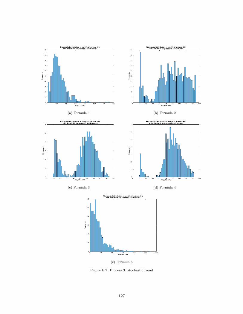
(a) Formula 1 (b) Formula 2

(c) Formula 3 (d) Formula 4

(e) Formula 5

Figure E.2: Process 3: stochastic trend

127

Appendix F

Risk-averse pricing, calibration of plain

vanilla bonds

Figure F.1: Calibration of default cases to match par value of plain vanilla bond: Process 1

128

Figure F.2: Calibration of default cases to match par value of plain vanilla bond: Process 2

Figure F.3: Calibration of default cases to match par value of plain vanilla bond: Process 3

129

Appendix G

Risk-averse pricing, indexed bonds with

default risk

130

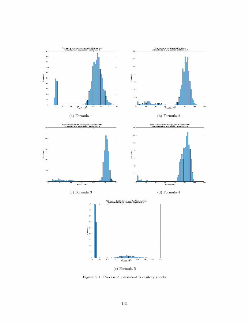
(a) Formula 1 (b) Formula 2

(c) Formula 3 (d) Formula 4

(e) Formula 5

Figure G.1: Process 2: persistent transitory shocks

131

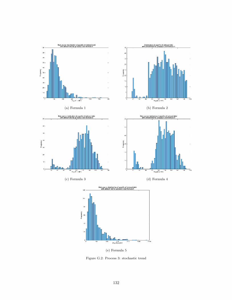
(a) Formula 1 (b) Formula 2

(c) Formula 3 (d) Formula 4

(e) Formula 5

Figure G.2: Process 3: stochastic trend

132

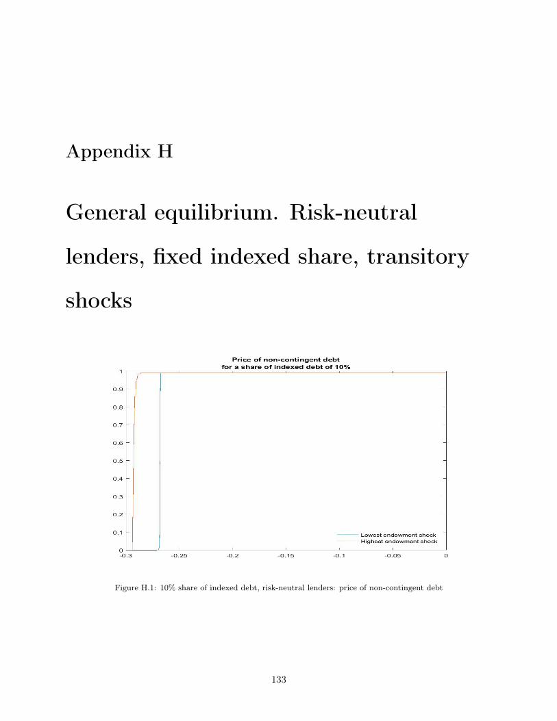
Appendix H

General equilibrium. Risk-neutral

lenders, fixed indexed share, transitory

shocks

Figure H.1: 10% share of indexed debt, risk-neutral lenders: price of non-contingent debt

133

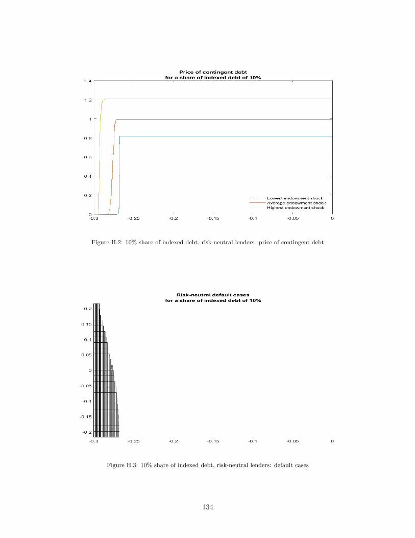
Figure H.2: 10% share of indexed debt, risk-neutral lenders: price of contingent debt

Figure H.3: 10% share of indexed debt, risk-neutral lenders: default cases

134

Figure H.4: 20% share of indexed debt, risk-neutral lenders: price of non-contingent debt

Figure H.5: 20% share of indexed debt, risk-neutral lenders: price of contingent debt

135

Figure H.6: 20% share of indexed debt, risk-neutral lenders: default cases

Figure H.7: 50% share of indexed debt, risk-neutral lenders: price of non-contingent debt

136

Figure H.8: 50% share of indexed debt, risk-neutral lenders: price of contingent debt

Figure H.9: 50% share of indexed debt, risk-neutral lenders: default cases

137

Appendix I

General equilibrium. Risk-neutral

lenders, fixed indexed share, stochastic

trend

Figure I.1: 10% share of indexed debt, risk-neutral lenders: price of non-contingent debt

138

Figure I.2: 10% share of indexed debt, risk-neutral lenders: price of contingent debt

Figure I.3: 10% share of indexed debt, risk-neutral lenders: default cases

139

Figure I.4: 20% share of indexed debt, risk-neutral lenders: price of non-contingent debt

Figure I.5: 20% share of indexed debt, risk-neutral lenders: price of contingent debt

140

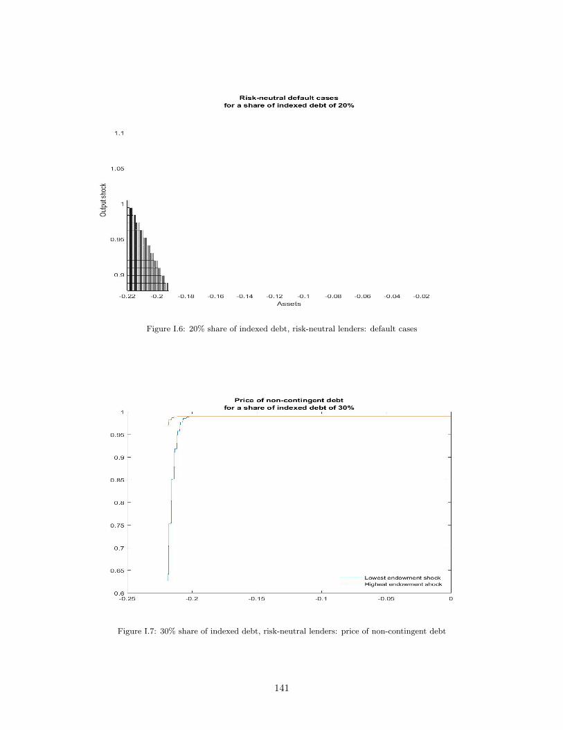
Figure I.6: 20% share of indexed debt, risk-neutral lenders: default cases

Figure I.7: 30% share of indexed debt, risk-neutral lenders: price of non-contingent debt

141

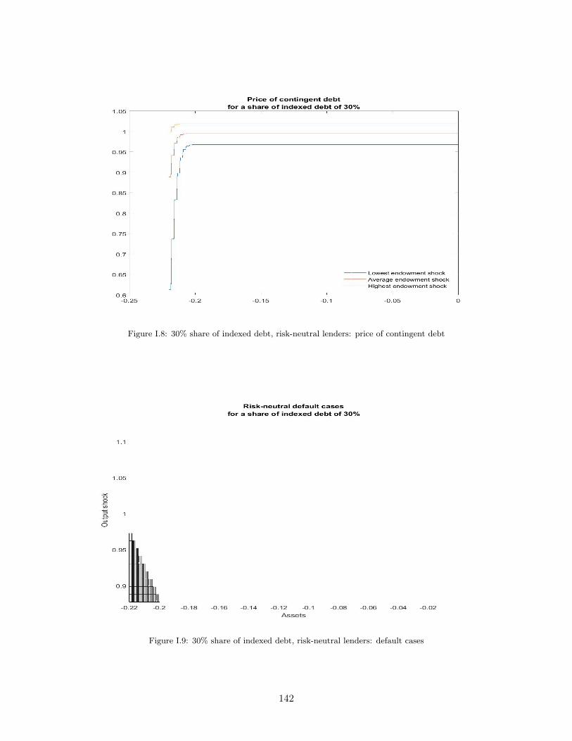
Figure I.8: 30% share of indexed debt, risk-neutral lenders: price of contingent debt

Figure I.9: 30% share of indexed debt, risk-neutral lenders: default cases

142

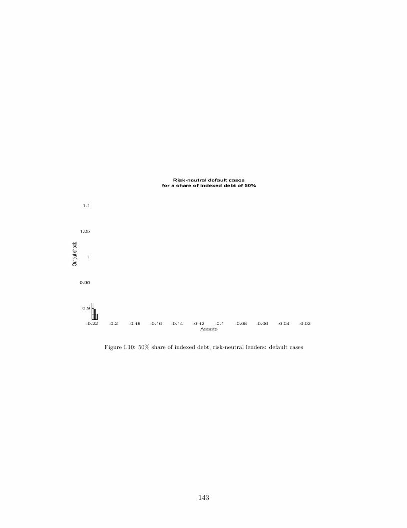
Figure I.10: 50% share of indexed debt, risk-neutral lenders: default cases

143

Appendix J

General equilibrium. Risk-neutral

lenders, endogenous share of indexed

debt, stochastic trend

Figure J.1: Lowest endowment shock: price of non-contingent debt

144

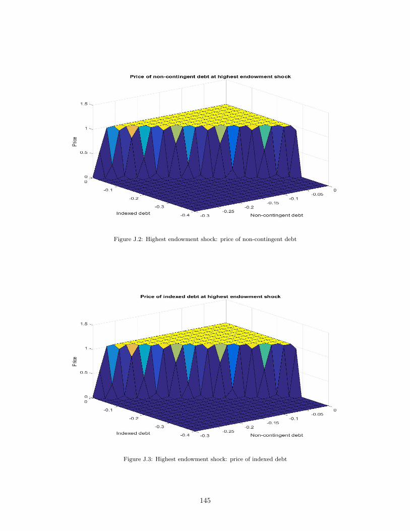
Figure J.2: Highest endowment shock: price of non-contingent debt

Figure J.3: Highest endowment shock: price of indexed debt

145

Appendix K

General equilibrium. Risk-neutral

lenders, endogenous share of indexed

debt, transitory shocks

Figure K.1: Lowest endowment shock: price of non-contingent debt

146

Figure K.2: Highest endowment shock: price of non-contingent debt

147

Appendix L

General equilibrium. Risk-averse

lenders, endogenous share of indexed

debt, stochastic trend

Figure L.1: Lowest endowment shock: price of non-contingent debt

148

Figure L.2: Highest endowment shock: price of non-contingent debt

Figure L.3: Lowest endowment shock: price of indexed debt

149

Figure L.4: Highest endowment shock: price of indexed debt

150

Appendix M

General equilibrium. Risk-averse

lenders, endogenous share of indexed

debt, transitory shocks

Figure M.1: Lowest endowment shock: price of non-contingent debt

151

Figure M.2: Highest endowment shock: price of non-contingent debt

Figure M.3: Lowest endowment shock: price of indexed debt

152

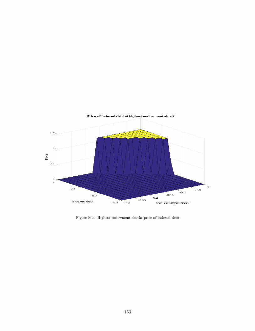
Figure M.4: Highest endowment shock: price of indexed debt

153