reaction wheels fault isolation onboard 3-axis controlled

International Journal of Prognostics and Health Management, ISSN 2153-2648, 2021

1

Reaction Wheels Fault Isolation Onboard 3-Axis Controlled Satellite using Enhanced Random Forest with Multidomain Features

Mofiyinoluwa O. Folami1, Afshin Rahimi2

1,2 Department of Mechanical, Automotive, and Materials Engineering, University of Windsor, Windsor, ON, N9B 3P4, Canada

[email protected] [email protected]

ABSTRACT

As the number of satellite launches increases each year, it is only natural that an interest in the safety and monitoring of these systems would increase as well. However, as a system becomes more complex, generating a high-fidelity model that accurately describes the system becomes complicated. There-fore, imploring a data-driven method can provide to be more beneficial for such applications. This research proposes a novel approach for data-driven machine learning techniques on the detection and isolation of nonlinear systems, with a case-study for an in-orbit closed loop-controlled satellite with reaction wheels as actuators. High-fidelity models of the 3-axis controlled satellite are employed to generate data for both nominal and faulty conditions of the reaction wheels. The generated simulation data is used as input for the isola-tion method, after which the data is pre-processed through feature extraction from a temporal, statistical, and spectral domain. The pre-processed features are then fed into various machine learning classifiers. Isolation results are validated with cross-validation, and model parameters are tuned using hyperparameter optimization. To validate the robustness of the proposed method, it is tested on three characterized da-tasets and three reaction wheel configurations, including standard four-wheel, three-orthogonal, and pyramid. The re-sults prove superior performance isolation accuracy for the system under study compared to previous studies using alter-native methods (Rahimi & Saadat, 2019, 2020).

1. INTRODUCTION

With the ever-growing number of satellites being launched into space, it is crucial that the health monitoring and safety of these systems be advanced enough to compensate for the lack of redundant components and their decreasing size. The attitude determination and control subsystem (ADCS), which employs reaction wheels (RWs) as actuators, is one of the

most critical components of a satellite subsystem. By accel-erating or decelerating the flywheels attached to the electric motor, RWs can correct the satellite’s orientation or perform maneuvers under disturbances (Rahimi et al., 2017). Smaller satellites require less cost for design and mass-production, meaning multiple can be launched into space at a time. There-fore, to ensure reliability and mission success, the health and maintenance of these systems are essential. As a result, fault detection and isolation (FDI) methods for ADCS has devel-oped great incentive to be improved and advanced.

The two main categories for FDI approaches are model-based and data-driven. In model-based approaches, the continuous comparison between the actual system state and nominal state is conducted and in turn, generates residuals. This is achieved by using a mathematical model of the system with ideal be-havior. One major advantage of this method is that it has the ability to provide a description of the dynamic behavior and physical understanding of the system (Tidriri et al., 2016). However, developing an accurate mathematical model that considers uncertainties and modeling errors is difficult due to some uncertainties being unquantifiable. As previously men-tioned, model-based methods compare the available data with prior information and generate residuals. One method of re-sidual generation is through observer-based techniques. If the system is observable (i.e., it is possible to determine the entire system behavior from the outputs) and the process parameters are known, then it is possible to estimate the output of a pro-cess with an observer and the residuals. In (Jia et al., 2019), two Non-Linear Observers (NLO) are developed to robustly reconstruct bias faults and effectiveness factors of RWs, and a systematic observer design method is obtained. Fault-toler-ant attitude control for the spacecraft system was not consid-ered in this study, however. Four classifiers, Random Forest (RF), SVM, Partial Least Squares (PLS), and Naïve Bayes (NB), are combined to create a fusion framework for FDI in RWs (Nozari et al., 2019). In (Nemati et al., 2019), nonlinear observers are used for fault diagnosis of spacecraft. The ob-servers are designed to ensure convergence of the estimation error to zero for the nominal nonlinear system. Fault isolation is achieved using a General Observer Scheme (GOS).

_____________________ Mofiyinoluwa Folami et al. This is an open-access article distributed under the terms of the Creative Commons Attribution 3.0 United States License, which permits unrestricted use, distribution, and reproduction in any me-dium, provided the original author and source are credited. https://doi.org/10.36001/IJPHM.2021.v12i2.3078

INTERNATIONAL JOURNAL OF PROGNOSTICS AND HEALTH MANAGEMENT

2

However, when dealing with model-based approaches, there are certain limiting factors such as system complexity, high dimensionality, nonlinearity processing.

Data-driven approaches focus on analyzing system outputs and rely immensely on large amounts of data, allowing these methods to perform well with large-scale and complex sys-tems, as well as reduce time and costs since the development of models is unnecessary. This approach can be beneficial if no mathematical model or expert knowledge about a system is available.

A highly nonlinear dynamic system is the result of modelling the complexity of a single RW. More RWs can be placed into the assembly combined with the attitude and dynamics of the satellite in orbit. If the parameters of interest are non-meas-urable to the FDI scheme, it becomes difficult to detect faults and isolate their root causes. When conducting data-driven FDI, there are two critical factors any scheme should have, 1) generation of a feature subset, 2) selection of the most opti-mal classifier. Research conducted by (ElDali & Kumar, 2021) proposed a growing neural network for aircraft engine fault diagnosis, detection, and prognostics. The model opti-mized the Long-Short Term Memory (LSTM) algorithm and was used to detect failure for RWs in the pyramid configura-tion. The model tried to detect failures in the four RWs by calculating a Health Index value. A value between 0 and 1, with the latter representing a greater chance of failure. The values were acquired from the residuals of the acquired speed values and the predicted ones. The study (Lee et al., 2020) addresses fault detection and identification in the RWs of nanosatellites based on a Deep Learning (DL) algorithm. Fault detection is accomplished using the residuals between the measured attitude and the estimated attitude. Trial and er-ror were used to optimize the learning and hyperparameters of the LSTM model used within this study. However, this technique did not consider the temporal elements of the atti-tude information and was more likely to misjudge because only the instantaneous values were used.

Most of the research above also involves instances where re-sidual generation is applied through analytical models. This method, however, does not do well in explaining the facility point behind the detected faults. Mixed learning models are limited to the performance of the best classifier used within the ensemble. If other classifiers have limitations, it can hin-der the overall accuracy of the method. Furthermore, most methods deal with only one RW and do not consider multiple faults or different RW assemblies. Based on the open litera-ture of past studies, a research objective was established. Which is the design and development of a data-driven FDI scheme that is capable of autonomously isolating the location of faults within a nonlinear system, with a case-study for an in-orbit closed-loop controlled satellite with reaction wheels as actuators This method is to be developed to be applicable to other systems, however it is being designed for this specific application. To achieve the above research objective, Time

Series Feature Extraction Library (TSFEL) transforms the time-domain data into a feature-space state. The new feature space is then fed as input into multiple machine learning models (MLMS). Sensitivity analysis of missing sensors, missing values and noise analysis was also conducted on var-ious datasets. The robustness of this method was also tested on three different configurations of the Reaction Wheel As-semblies (RWA). Lastly, k-fold cross-validation is used to validate the results. The choice for using less computationally expensive methods versus more advanced and highly compu-tational methods was made to ensure applicability and acces-sibility of the proposed in this study on a broader range of satellite units with lower-end computational capacities. This is particularly important as smaller satellites with limited ca-pacity may not house supercomputers onboard, and compu-tational power and energy consumption can be limiting fac-tors in deploying such algorithms for the FDI of such units.

Past research on data-driven approaches shows that these methods are known to have some limitations. The proposed method can deal with the extensive consumption of re-sources, memory, and algorithmic complexity by applying a hierarchical approach to enhance the isolation scheme and only utilizing the appropriate resources when required.

The novelties of this approach are:

1. Based on previous assessments, common feature subsets such as statistical features do not result in the best results. Therefore, an automated feature extraction library is used to obtain the best feature subset from a temporal, statistical, and spectral domain which has not been ex-plored for this specific application, to represent the char-acteristics of the multiple in-phase faults from different points of view and where most literature only consider one space-state transformation.

2. Consideration of three different fault time characteris-tics: Abrupt, Transient, and a general case. Where most literature mainly considers abrupt faults.

3. Use of variable inception time and duration of the faults for different cases to tackle the applicability range of data-driven methods and broaden the scope, where other literature only considers constants.

4. Classification of multiple in-phase faults where other lit-erature primarily considers either single faults or multi-ple out-of-phase faults.

The remainder of this paper is organized as follows: Section 2 presents the problem definition. Section 3 explains the methodology employed in the study. Section 4 presents the case studies used to evaluate the proposed method. Section 5 offers insight into the results and discussion of the study. Sec-tion 6 concludes the paper with final remarks.

2. PROBLEM DEFINITION

A nonlinear system in discrete-time state space can be repre-sented in Eq. (1)


3

𝛺 = #𝜉!"# = 𝑓(𝜉! , 𝑢! , 𝜃! , 𝑤!

$)𝜃!"# =𝜃! +𝑤!%

𝑦! = 𝑔(𝜉! , 𝜃!) + 𝜈!

(1)

where at time step 𝑘, 𝜉! ∈ ℝ& is the state vector, 𝑢𝑘 ∈ ℝ' depicts the control input vector, 𝜃! ∈ ℝ( , 𝑦! ∈ ℝ' , 𝑤!

$ ∈ℝ& , 𝑤!% ∈ 𝑅( and 𝑣𝑘 ∈ ℝ' represent the system parame-ter vector, measurement vector, additive process noise for states, additive process noise for parameters, and additive measurement noise, respectively. 𝑓(∙) is a nonlinear process model, and 𝑔(∙) is a nonlinear measurement model. Full state measurement 𝑦! = 𝜉! + 𝑣! is considered. In this study, it is under the assumption that the system component faults are reflected as changes in the physical system parameters (Sobhani-Tehrani et al., 2014). Eq. (2) describes the faulty system, also known as a multi-parameter fault model, with:

𝜃! =𝜃) + 𝛼! (2)

where 𝜃) ∈ ℝ(is the nominal parameter vector representa-tion andthe fault parameter vector containing L fault ele-ments is represented by 𝛼! ∈ ℝ*. By using the fault model given by Eq. (2), one can transform the problem of nonlinear fault diagnosis into the form of an on-line nonlinear parame-ter tracking problem. Furthermore, for fault isolation, one can extract 𝐿 single-parameter models Ωi 𝑖 = 1, … , 𝐿 . This is shown in Eq. (3) below:

Ω+: 𝜃!+ =𝜃)+ + 𝛼!+ 𝑖 = 1,… , 𝐿 (3)

The mission of the data-driven algorithm is set to classify the current state of the system as one of the possible 𝐿 faulty cases. In this study, multiple fault scenarios are considered.

3. METHODOLOGY

A hierarchical approach is used within this study for the methodology when tackling the FDI problem. This ensures a reduction in computation time by allocating the right re-sources to be used only when required. A data-driven fault diagnosis model is created to classify multiple in-phase faults of a satellite RW. The data is simulated using RW data and then extracted for features. The features are calculated using TSFEL and then reduced using Recursive Feature Elimina-tion (RFE) (Bahl et al., 2019) to produce a feature subset ranking. The features are fed as input for the machine learn-ing model (MLM) as inputs for training and testing. The MLMs implemented within this study include Gradient Boosting (GB), Decision Tree (DT), Random Forest (RF), and Multi-Layer Perceptron. The final step includes employ-ing tenfold – cross-validation to provide a more robust esti-mation of feature selection.

3.1. Data Preprocessing

It requires much time and effort for data science experts to model the Machine Learning Models (MLM) and tune its hy-perparameters. For some spacecraft systems, historical data

is not always available for training because the data is being collected in real-time. This puts a limitation on the model’s time to tune and train the algorithm. It also makes onboard health monitoring a difficult task since the model would have to be created after the data is transmitted to Earth. Auto-ma-chine learning can compensate for the drawbacks of normal machine learning techniques by automating the data pre-pro-cessing, model selection, hyperparameter optimization and the interpretation of the results. To assist the MLM in accu-rately distinguishing between nominal and fault scenarios, the time-series data is transformed into a feature space state. The features are acquired from raw time series data through Python package TSFEL, which extracts over 60 different fea-tures across a spectral, temporal, and statistical domain (Barandas et al., 2020). The new representation of the data is what is used as input for the training set. The data is also fil-tered for missing values, highly correlated features, and low variance features. Finally, the data is normalized before being fed into the MLMs.

3.2. Feature Reduction

Less sensitive and inaccurate features can reduce the model’s ability to predict faults accurately. That is why Recursive Feature Elimination Cross-Validation (RFECV) was imple-mented in the pre-processing stages. RFECV is an iterative backward selection method that uses a classification model to produce a feature subset ranking instead of a feature ranking. All the features are fitted to the model, and at each iteration, the feature with the least importance is eliminated (Ramachandran & Siddique, 2019). For this study, RF is used to train the model, and for each tree, the model estimates the variable importance by recording the out-of-bag prediction accuracy for every predictor variable premutation. The dif-ference between the prior and the altered model accuracy is averaged over all trees and normalized by the standard error at each iteration. The results for RFECV determined that the optimal number of features was 22, as shown in Figure 1.

Figure 1. Recursive feature elimination


4

3.3. Machine Model Selection

In this section, the various machine learning models imple-mented during the study are briefly discussed. Gradient Boosting (GB) (Bentéjac et al., 2021) is a machine learning technique utilized for regression or classification. This is done by constructing a prediction model comprising an en-semble of weaker models (i.e., Decision Tree). The objective of the GB is to minimize the loss between the actual class value and the predicted class value. The Random Forest (RF) (Probst et al., 2019) classifier consists of many individual de-cision trees that operate as an ensemble. Each tree will return a class, and the class with the most votes becomes the model’s prediction. The low correlation between the trees makes RF a helpful classifier. This protects each tree from errors of other individual trees. A Decision Tree (DT) learns from data to try and approximate a sine curve (Charbuty & Abdulazeez, 2021). This curve has a set of if-then-else deci-sion rules. It breaks down data into smaller subsets while in the same notion incrementally making an associated DT. To enhance the RF and DT classifiers, a meta-classifier Ada-Boost is used. It begins by fitting the classifier on the original data set and continues to fit additional copies of the classifier on the original data. However, in successive iterations, the weights of the incorrectly classified instances are adjusted to achieve better classification. The Multi-Layer Perceptron (MLP) is a feed-forward Artificial Neural Network (ANN) (Mishra & Huhtala, 2019). It can be referred to as a network with multiple layers of perceptron (nodes), each with a threshold activation function. There are at least three layers of nodes in an MLP: input layer, hidden layer, and output layer. Besides the input layer, each node uses a non-linear ac-tivation function. Backpropagation is used for training. The hyperparameters for the MLP were tuned using GridsearchCV to run each model with different hyperparam-eters and return the one with the optimal hyperparameters.

3.3.1. Training, Testing, and Validation

The input data was trained and tested at various splits. After a series of runs, an 80:20 train-test split resulted in the best performance for the MLMs. The K-fold cross-validation technique is also implemented to evaluate predictive models by partitioning the original samples into a training set and test set. The benefit of this method is that all observations are

used for both training and validation, and each observation is used for validation only once.

In the following section, details on a case-study are provided to evaluate the performance of the proposed methodology.

4. CASE STUDY: FAULT ISOLATION OF SATELLITE RWS

To assess the performance of the proposed FDI method, the faults for RWs onboard a 3-axis controlled satellite are em-ployed. The simulation consists of a high-fidelity nonlinear model of the RW, nonlinear satellite attitude dynamics, and a sliding mode controller (SMC), depicted in Figure 2. It should be noted that in this study, the simulation setup is as-sumed to have a perfect sensor, and there is no estimator, so the noise system output feeds directly back into the sum junc-tion before the controller. In the following sections, the effect of noise in system measurement is studied under sensitivity analysis discussions for the proposed method. Each compo-nent for this case study can be detailed as follows:

4.1.1. Satellite Dynamics

A fully actuated rigid body spacecraft with RWs as actuators under external and internal torques can be expressed as:

𝐽,-, = −𝜔,-, × (𝐽.𝜔,-, + 𝐴/0𝐽1Ω) − 𝐴𝜏/0 + 𝜏2 (4) where 𝐽. ∈ ℝ343 is the spacecraft’s moment of inertia in-cluding the RWs and 𝐽 is defined as 𝐽 = 𝐽. − 𝐴𝐽1𝐴5 , 𝐽1 ∈ℝ646 = 𝑑𝑖𝑎𝑔([𝐽1#,𝐽18, 𝐽13, 𝐽16]) stands for the axial mo-ment of inertia of each RW. the mapping matrix 𝐴 ∈ 𝑅346 captures the influence of the actuator’s toques to the principal axes of the spacecraft. Angular velocity of the spacecraft rel-ative to the inertial frame expressed in the body frame is de-noted by 𝜔,-, . The external torque is represented by 𝜏2 ∈ℝ34# and the torque generated by the RW is 𝜏/0. Using qua-ternions, the kinematic equation for the spacecraft can be for-mulated as:

J𝑞:6L =

12 J𝑞6𝐼 + 𝑞:×

−𝑞:5L𝜔,*, (5)

where the unit quaternion is represented by O𝑞:𝑞6P with 𝑞: ∈

ℝ34# = [𝑞#, 𝑞8, 𝑞3]5 and 𝑞6 ∈ ℝ representing the Euler pa-rameters that portray the spacecraft body frame orientation with respect to the orbital frame, where 𝑞:5𝑞: + 𝑞68 = 1. The

Figure 2. Proposed FDI simulation setup

Controller(SMC)

Actuators(RW)

SpacecraftDynamics and

Kinematics

Desired Attitude

-+

Control Command

Control Torque

Spacecraft Attitude

Disturbance Torques

+_e u

ctydy

et

( , )d dqw ( , )qw


5

identity matrix is I ∈ ℝ343 and the skew-symmetric matrix of the quaternion vector 𝑞:× is expressed as:

𝑞:× = Q0 −𝑞3 𝑞8𝑞3 0 −𝑞#−𝑞3 𝑞# 0

S (6)

4.1.2. Controller

A simplified nonlinear sliding mode controller with quater-nion tracking error is defined as (Kumar et al., 2018):

𝑞2 = 𝑞<6𝑞: − 𝑞6𝑞<: + 𝑞:×𝑞<:𝑞26 =𝑞<6𝑞6 + 𝑞<:5 𝑞:

(7)

where 𝑞<: ∈ 𝑅34# and 𝑞<6 ∈ 𝑅 and are the desired attitude, and 𝑞25𝑞2 + 𝑞628 = 1. The rotation matrix is given by:

𝐶2 = (𝑞628 − 𝑞25𝑞2)𝐼 + 2𝑞25𝑞2 − 2𝑞62𝑞2× (8) Here 𝐶25𝐶2 = 1 , 𝐶2 = −𝜔2×𝐶2 . Relative angular velocity 𝜔2 ∈ 𝑅34# is formulated as follows:

𝜔2 =𝜔,*, + 𝐶2𝜔< (9) where 𝜔< ∈ 𝑅34# denotes the desired angular velocity. The required control command is defined as:

𝑢= = −𝜂𝐴5 >‖>‖

, 𝜂 = 𝑝@ + 𝑝#‖𝑋‖ (10)

where 𝑝@ and 𝑝# are positive constants and 𝑋 ∈ 𝑅A4# =[𝑞:, 𝜔,*, ]5. The simplified required input can now be calcu-lated for the actuator given actuator dynamics and required control command as (Kumar, 2018):

𝑉B)'' = 𝑅C𝐾DE#𝑢= (11) where 𝑉B)'' ∈ 𝑅6×# is the voltage input to the RWs, 𝑅C ∈𝑅6×6 = 𝑑𝑖𝑎𝑔([𝑟C#, 𝑟C8, 𝑟C3, 𝑟C6]) is the armature resistance in ohm and 𝐾D ∈ 𝑅6×6 = 𝑑𝑖𝑎𝑔([𝑘D#, 𝑘D8, 𝑘D3, 𝑘D6])is the motor torque constant for the RWs. All control parameters includ-ing 𝜆, 𝑝@ and 𝑝# are set to the value of 1 for the required sim-ulations in this case study. The full derivation of this control-ler can be found in (Godard, 2010) on pages 113 to 115.

4.1.3. Actuator

The RW used in this study is an ITHACO “’ type A’” by Goodrich. A high fidelity RW nonlinear model was obtained from Bialke (Bialke, 1998) and was integrated into the ACS dynamics. The RW nonlinear model, including discontinuous functions approximated by sinusoidal functions, can be for-mulated as:

𝐼/0 = 𝐺<𝜔<[𝑓3(𝜔, 𝐼/0) − 𝑓F(𝜔)] − 𝜔<𝐼/0+𝐺<𝜔<𝑉B)''

/0 =1𝐽1𝑓#(𝜔) + 𝐾D𝐼/0[𝑓8(𝜔) + 1] − 𝜏:𝜔

−𝜏B𝑓6(𝜔) + 𝜏&)+.2

(12)

where 𝑓# and 𝑓8 represent the motor disturbance, 𝑓3 denotes the EMF torque-limiting block. The variables 𝑓6 , 𝑓F and

𝑉B)'' represent the analytical approximation of the sign function in the Coulomb friction block, speed limiter block and torque command voltage, respectively.

4.1.4. Reaction Wheel

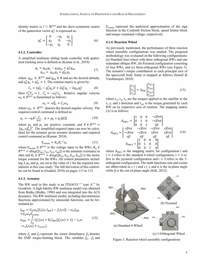
As previously mentioned, the performance of three reaction wheel assembly configurations was studied. The proposed methodology was evaluated on the following configurations: (a) Standard four-wheel with three orthogonal RWs and one redundant oblique RW, (b) Pyramid configuration consisting of four RWs, and (c) three-orthogonal RWs (see Figure 3). The actuator’s torque contribution to each principal axis of the spacecraft body frame is mapped as follows (Ismail & Varatharajoo, 2010):

Q𝜏4𝜏G𝜏HS = 𝐴/0 _

𝜏1#𝜏18𝜏13𝜏16

` (13)

where 𝜏4 , 𝜏G, 𝜏H are the torques applied to the satellite in the x, y, and z direction and 𝜏1+ is the torque generated by each RW on its respective axis of rotation. The mapping matrix (A) is as follows:

𝐴/0# = Q1 0 00 1 00 0 1

−𝑐𝛽𝑠𝛼−𝑐𝛽𝑠𝛼𝑠𝛽

S

𝐴/08 = Q𝑐𝛽𝑠𝛼 −𝑐𝛽𝑐𝛼 −𝑐𝛽𝑠𝛼−𝑐𝛽𝑠𝛼 −𝑐𝛽𝑐𝛼 𝑐𝛽𝑐𝛼𝑠𝛽 𝑠𝛽 𝑠𝛽

𝑐𝛽𝑠𝛼𝑐𝛽𝑐𝛼𝑠𝛽

S

𝐴/03 = Q1 0 00 1 00 0 1

000S

(14)

where 𝐴/0+ is the mapping matrix for configuration 𝑖 and 𝑖 = 1refers to the standard 4-wheel configuration, 𝑖 = 2 re-fers to the pyramid configuration and 𝑖 = 3 refers to the 3-orthogonal configuration. The math functions sine and cosine are abbreviated as c (·) and s (·), and α is the in-plane angle while β is the out-of-plane angle (Kök, 2012).

(a) Standard 4-Wheel

(b) Pyramid

(c) 3-Orthogonal Wheel

Figure 3. Reaction wheel assembly configurations

RW1

RW2 RW1

RW2

RW3

RW4

β

α

RW2

RW4

RW1RW3

β

RW1

RW2

RW3


6

For the three-orthogonal wheel configuration, a separate da-taset had to be generated to account for the proper number of RWs engaged. Cases 1-3 shown in Table 2 referenced in sec-tion 4.1.5 are identical to the datasets constructed for the standard and pyramid configurations except for fewer reac-tions wheels, resulting in a lower number of fault combina-tions.

4.1.5. Fault Formation

The simulation data is obtained from a closed-loop ACS sim-ulation of a three-axis stabilized low earth orbit (LEO) satel-lite. Abrupt and transient time-varying fault cases, as well as a generalized fault case, are added into two of the RW com-ponents as variations via the bus voltage (𝑉𝑏𝑢𝑠) and motor torque back electromotive force (BEMF) constant ( 𝑘𝑡 ). 𝑉𝑏𝑢𝑠and kt are modelled as the voltage drop of the power bus and the variations in the torque gain, respectively. The multi-parametrized fault model is obtained by replacing 𝑉𝑏𝑢𝑠, 𝑗 with 𝑉𝑏𝑢𝑠, 𝑗0 + 𝛼𝑗1 and 𝑘𝑡, 𝑗 with 𝑘𝑡, 𝑗0 + 𝛼𝑗2 , where j is the index for the RW unit among the units consid-ered and 𝛼I+ are unknown fault parameters, indicating a pos-sible fault in either the bus voltage or motor current of each wheel. The value for 𝛼I+ will be zero at any given time due to the additive form of the fault parameters. Any deviation from zero for any fault parameter would indicate the fault size and its severity. Within this study, only system satellite outputs, namely 𝑞 and 𝜔 are observed for faulty behavior. Abrupt faults can be viewed as instantaneous faults and can lead to complete failure of the system. Transient faults are more tem-porary faults within the system and may return to normal pa-rameters given a certain amount of time. This study investi-gates the effect of fault duration, inception of the fault, and severity of faults during a mission. The initial moment the fault is introduced into the system can be described as the in-ception time. Duration is the length of time the fault remains within the system. Lastly, the severity denotes the magnitude by which the faulty parameter has deviated from its nominal values during the fault period. With these definitions in mind, three datasets are created when evaluating the proposed methods:

1. Case 1 (abrupt fault): The inception time for the faults in both 𝑉𝑏𝑢𝑠 and𝑘𝑡 are set at a random value 𝑡+ ∈ (0,10) seconds and the duration of these faults is defined from the inception time to the end of the simulation.

2. Case 2 (transient bounded fault): Inception time for faults in both 𝑉𝑏𝑢𝑠and 𝑘𝑡 are set at a random value 𝑡+ ∈(0,10) seconds and the duration of these faults are set randomly within 𝑡< ∈ (10,20) second range.

3. Case 3 (transient unbounded fault): The inception time for faults in 𝑉𝑏𝑢𝑠and 𝑘𝑡 are set at a random value 𝑡+ ∈(5,55) seconds and the duration of each fault is deter-mined randomly within 𝑡< ∈ (5,60 − 𝑡+) to not exceed the total simulation of 60 seconds.

All cases include a random combination of 𝑘D and 𝑉JK. faults, with a random severity for each with a set fault devia-tion range presented in Table 1. The difference in the fault definitions for Cases 2 and 3 lie within the definition of their fault inception time and duration. The larger inception time for Case 3 creates a broader scope or window for fault incep-tion, which is a better representation of real-world scenarios. This distinction for cases 2 and 3 makes them more complex.

Description Case 1 Case 2 Case 3 Unit Fault Scenario 0-15/0-7 0-15/0-7 0-15/0-7 integer 𝑘D in fault 0/1 0/1 0/1 binary 𝑉JK.in fault 0/1 0/1 0/1 binary 𝑘Dinception 0-10 0-10 5-55 sec 𝑉JK. inception 0-10 0-10 5-55 sec 𝑘D duration 0-60 10-20 ∗ sec 𝑉JK. duration 0-60 10-20 ∗ sec 𝑘D severity 29 ± 2 29 ± 2 29 ± 2 mN·m/A 𝑉JK. severity 6 ± 2 6 ± 2 6 ± 2 Volt

Table 1. Fault scenario input format

4.1.6. Dataset Structure

This section provides details of the dataset used for this study.

4.1.6.1 Raw Data As previously mentioned, it is assumed that the faults injected into the RW units can be detected and isolated by evaluating the satellite output parameters. The satellite attitude parame-ters include quaternions, 𝑞# to 𝑞6 , and angular speed 𝜔#to 𝜔3. Based on the desired conditions for the case scenarios presented in section 4.5, input values are fed into the MATLAB simulator, which returns the raw data used as input for the FDI algorithm. For this study, 5,000 simulations per scenario were run to create a data set, and since there are 16 scenarios, 80,000 simulations were collected to create one da-taset. Since the data pertaining to 𝑞6 is not independent of 𝑞# to 𝑞3 they were omitted when fed into the FDI algorithm dur-ing the pre-processing stage. Of the 80,000 CSV files stored, each one contains a data set of simulation time step of 0.1 seconds, and each simulation has a time length of 60 seconds; therefore, 600 rows are generated. The number of columns is determined as 2 × 8 = 16 for two sets of 4 parameters re-lated to the nominal and faulty parameters. This raw data is later transformed into the three different domains through TSFEL, which extracts features from a spectral, statistical, and temporal domain as previously mentioned, and ulti-mately is fed into the MLMs. Combination theory is used to calculate the total number of combinations for a four-wheel and three-wheel RW assembly, which can be seen in Eq. (15)

𝐿 = lm𝑛𝑝o = l

𝑛!𝑝! (𝑛 − 𝑝)!

&

LM#

&

LM#

(15)

where 𝑝 is the number of faulty units at time step 𝑘, and 𝑛 is the number of available units that could become faulty. To be


7

able to refer to each combination (fault scenario), all possible cases are assigned a number in Table 2 for each RW wheel assembly configuration. The fault scenarios for the standard four-wheel and pyramid configurations are the same, while because of the number of wheels involved in the assembly, the scenario numbers and combinations are different for the 3-orthogonal assembly. Once the simulations are executed via the inputs for fault scenarios in Table 1 and the satellite ACS setup in Figure 2, the satellite measurables q and ω are stored in comma-separated value (CVS) files for each simu-lation separately in the format presented in Table 2 where FW refers to faulty wheels. All the CSV files are used as input for training and testing the MLMs to evaluate their performance under the proposed method and compare their merits.

Configuration No. FW No. FW Standard or Pyramid 0 None 8 2,3 1 1 9 2,4

2 2 10 3,4 3 3 11 1,2,3 4 4 12 1,2,4 5 1,2 13 1,3,4 6 1,3 14 2,3,4 7 1,4 15 1,2,3,4

3-Orthogonal 0 None 4 1,2 1 1 5 1,3 2 2 6 2,3 3 3 7 1,2,3

Table 2. Fault scenarios for RW assemblies

Item Unit Description Time sec time in simulation 𝑞+,N2C(DNG - nominal quaternion 𝜔+,N2C(DNG rad/sec nominal angular speed for satellite 𝐼/0,+N2C(DNG A nominal current of 𝑅𝑊+ 𝜔/0+,N2C(DNG rad/sec nominal angular speed of 𝑅𝑊+ 𝑞+,OCK(DG - faulty quaternion 𝜔+,OCK(DG rad/sec faulty angular speed for satellite 𝐼/0+,OCK(DG A faulty current of 𝑅𝑊+ 𝜔/0+,OCK(DG rad/sec faulty angular speed of 𝑅𝑊+

Table 3. RW simulation outputs

5. RESULTS AND DISCUSSION

The accuracy of classification methods, as discussed in Sec-tion 3, which is employed for the FDI problem discussed in Section 2 for the data acquired in the case study detailed in Section 4, is presented in, Table 4, Table 5, and Table 6.

The simulation is tested at a size of 20%. For the cross-vali-dation, the random forest classifier was employed to save on computational costs, the splitting strategy was set to 10-folds, and the parameter that was varied in this analysis was the max depth of the trees.

Method Case 1 (%) Case 2 (%) Case 3 (%) Gradient Boosting 98.56 80.86 24.64 Random Forest 98.91 69.61 24.36 Decision Tree 92.32 59.14 19.20 MLP 85.64 69.16 21.78

Table 4. Standard 4-wheel configuration accuracy

Method Case 1 (%) Case 2 (%) Case 3 (%) Gradient Boosting 97.87 51.31 51.65 Random Forest 96.82 54.64 56.05 Decision Tree 93.66 42.19 42.91 MLP 81.42 32.92 32.27

Table 5. Pyramid configuration accuracy

Method Case 1 (%) Case 2 (%) Case 3 (%)

Gradient Boosting 98.02 90.20 36.78 Random Forest 97.65 88.5 35.64 Decision Tree 94.18 83.20 29.77 MLP 94.16 78.2 26.34

Table 6. 3-Orthogonal configuration accuracy

From the results listed in the tables above, the classifier’s ability to predict is significantly affected by the fault severity and duration definitions given with the scope of the simulated time series. The case definition described in Section 4.1.5 shows that case 3 is below adequate for any real-world appli-cations. This can be anticipated due to a combination of 1) the fault inception time initiating nearing the end of the sim-ulation time and 2) the fault duration being relatively short. These two problems stem from the influence of the controller. Since the controller compensates for the system when detect-ing a fault, if the inception time and duration of the fault are not distinct enough, then the system has a hard time classify-ing the faults. In practical applications of in-orbit satellites, cases 1 and 2 are more practical. If a commanded orientation change causes a fault to occur, the fault will most likely per-sist to the following command, representing the cases out-lined in section 4.1.5. If the MLM fails to identify the fault during a maneuver, the fault will be present in the following command, leading to a true-positive prediction. The learning curves, validation curves, and precision-recall graphs can be seen in Appendix A.

It should also be mentioned that the configuration of the RW assembly influences the accuracy of the proposed method. It is expected that the overall accuracy of the cases for the three-orthogonal wheel, standard four-wheel, and pyramid go from best to worst, respectively. This is due to the placement of the RWs or the lack of a redundant RW component. Since the three-orthogonal wheel configuration only has three wheels


8

on individual axes, it is not affected by the moments gener-ated by the other RWs. Therefore, if there is a sudden change in the torque generated, there should be a more direct effect on the satellite’s behavior. However, this is not the case for the other configurations since the torque generated by these RWs is proportionally changing or contributing to the x, y, and z axes, which results in some direct effect from the three RWs on the x, y and z axes and some indirect contributions from the fourth wheel. The pyramid configuration has a more challenging time with this proposed method due to its assem-bly’s symmetry. If there is an abnormality in the first two RWs and the same discrepancy occurs in the other two RWs the system will have difficulty distinguishing between the two faults.

5.1. Confusion Matrices

The model’s performance is evaluated using the test data and used to construct the con-fusion matrices with more details per each scenario. To normalize the results, the number of instances tested per class is used. The results for the confu-sion matrices are demonstrated in Table 7, Table 8, and Table 8.

Act

ual

0 146 0 0 0 0 0 0 0 0 0 0 0 0 0 0 0 1 0 134 0 0 0 0 0 1 0 0 0 0 0 0 0 0 2 0 0 146 0 0 0 0 0 1 0 0 0 0 0 0 0 3 0 0 0 148 0 0 0 0 0 0 0 0 0 0 0 0 4 0 0 0 1 131 0 0 0 0 0 0 0 0 0 0 0 5 0 0 0 0 0 153 0 0 0 0 0 0 0 0 0 0 6 0 1 0 0 0 0 150 1 0 0 0 0 0 0 0 0 7 0 0 0 0 0 0 0 144 0 0 0 0 0 0 0 0 8 0 0 0 0 0 0 0 0 144 0 0 0 0 0 0 0 9 0 0 0 0 0 0 0 0 2 146 0 0 0 0 4 0

10 0 0 0 6 0 0 0 0 0 0 157 0 0 0 0 0 11 0 0 0 0 0 0 0 0 0 0 0 164 0 0 0 2 12 0 0 0 0 0 0 0 0 0 0 0 1 149 0 0 0 13 0 0 0 0 0 0 1 0 0 0 0 0 0 152 0 0 14 0 0 0 0 0 0 0 0 0 1 0 0 0 0 152 0 15 0 0 0 0 0 0 0 0 0 0 0 0 0 0 0 162

0 1 2 3 4 5 6 7 8 9 10 11 12 13 14 15 Predicted

Table 7. Confusion matrix for standard 4-wheel

Along the diagonal, the values that depict the percentage of instances correctly predicted can be seen. Scenario 0 refers to the conditions where all RW units are healthy, and the 100% accuracy establishes the learner’s ability to distinguish be-tween nominal and faulty conditions. Scenario 0-4 represents the single faults of the RW where only one unit can fail. Within these sections of the confusion matrices shown above, there is at most only one misclassification amongst the clas-ses. This provides great confidence in the methodology to identify single faults at the very least correctly. The remain-der of the scenarios pertain to the definitions described in Ta-ble 2. As more units fail simultaneously, the performance of the classifier slightly degrades. This can be explained due to the impact of multiple faulty units on the overall system

behavior. As the predictions are made based on the system-level measurements (i.e., satellite quaternions and angular ve-locities), it is expected for the predictors to identify similar behavior as contributed to by similar actuator faults. There-fore, in any fault scenario, the system-level impact from ac-tuator faults is similar, the predictors will identify them as the same scenario and this can become more evident as more ac-tuator units become faculty simultaneously.

Act

ual

0 105 0 0 0 0 0 0 0 0 0 0 0 0 0 0 0 1 0 94 0 0 0 0 0 0 0 0 0 0 0 0 0 0 2 0 0 90 0 0 3 0 0 0 0 0 0 0 0 0 0 3 0 0 0 91 0 0 2 0 0 0 0 0 0 0 0 0 4 0 0 0 0 90 0 0 8 0 0 0 0 0 0 0 0 5 0 0 3 0 0 93 0 0 0 0 0 0 0 0 0 0 6 0 0 0 2 0 0 95 0 0 0 0 0 0 0 0 0 7 0 0 0 0 4 0 0 94 0 0 0 0 0 0 0 0 8 0 0 0 0 0 0 0 0 88 0 0 6 0 0 0 0 9 0 0 0 0 0 0 0 0 0 88 0 0 2 0 0 0 10 0 0 0 0 0 0 0 0 0 0 110 0 0 0 0 0 11 0 0 0 0 0 0 0 0 1 0 0 89 0 0 0 0 12 0 0 1 0 0 0 0 0 0 8 0 0 112 0 0 0 13 0 0 0 0 0 0 0 0 0 0 8 0 0 89 0 0 14 0 0 0 0 0 0 0 0 0 0 0 0 0 0 99 5 15 0 0 0 0 0 0 0 0 0 0 0 0 0 0 1 108

0 1 2 3 4 5 6 7 8 9 10 11 12 13 14 15 Predicted

Table 8. Confusion matrix for pyramid

Act

ual

0 107 0 0 0 0 0 0 0 1 0 92 0 0 6 0 0 0 2 0 0 79 0 0 0 0 0 3 0 0 0 98 0 0 3 0 4 0 2 0 0 94 0 0 1 5 0 0 0 0 0 91 0 5 6 0 0 0 0 0 0 91 0 7 0 0 0 0 0 9 0 87

0 1 2 3 4 5 6 7 Predicted

Table 9. Confusion matrix for 3-axis orthogonal

5.2. Sensitivity Analysis

Although many MLMs were tested against the proposed method to simplify analysis results, only one machine learn-ing classifier was used for sensitivity analysis. The model’s sensitivity is evaluated for missing values, missing sensors, and noise.

5.2.1. Noise Analysis

To study the effects of noisy raw data on the model’s perfor-mance, Gaussian noise was added at multiple signal-to-noise ratios. Gaussian noise with a zero mean was added during the


9

study. Table 10, Table 11, and Table 12 show the results for the different levels of SNR on the GB classifier. Through the results, it is seen that the model’s performance decreases as the SNR decreases. The model contains a reasonable accu-racy above 40 dB for the abrupt fault case, which is of greater importance to practical applications.

Standard 4-Wheel SNR (dB) 60 50 40 30 20 10 None Score (%) 99.2 98.8 98.4 91.3 75.1 54.7 99.2

3-Orthogonal Wheel SNR (dB) 60 50 40 30 20 10 None Score (%) 94.7 93.3 92.3 87.4 76.3 58.2 97.6

Pyramid SNR (dB) 60 50 40 30 20 10 None Score (%) 97.3 97.0 96.7 90.8 72.3 48.6 96.8

Table 10. Noise analysis for Case 1 (abrupt fault case)




Table 11. Noise analysis for Case 2 (transient fault case)




Table 12. Noise analysis for Case 3 (general fault case)

5.2.2. Missing Sensor Analysis

For this missing sensor analysis, the fault isolation method was tested under the assumption that not all sensors provide full measurement during the system’s operation. Therefore, measurements from some of the sensors are missing due to one or multiple failed sensors. Sensor readings are repre-sented by the satellite quaternions (𝑞#, 𝑞8, 𝑞3) and angular ve-locities (𝜔#, 𝜔8, 𝜔3) and the results for the analysis can be seen in Table 13, Table 14, and Table 15, respectively. In each of these tables, various combinations of working sensors (available measurements) are provided along with the

isolation method accuracy for the various severity cases in-troduced in Section 4.1.5 (i.e., Cases 1, 2, and 3).

Available Sensors Case 1 Case 2 Case 3 Score (%) Score (%) Score (%) 𝑞8, 𝑞3, 𝑞6, 𝜔#, 𝜔8, 𝜔3 99.04 73.40 11.84 𝑞#, 𝑞3, 𝑞6, 𝜔#, 𝜔8, 𝜔3 99.16 70.44 11.47 𝑞#, 𝑞8, 𝑞6, 𝜔#, 𝜔8, 𝜔3 97.96 73.78 12.90 𝑞#, 𝑞8, 𝑞3, 𝜔#, 𝜔8, 𝜔3 98.79 73.28 13.90 𝑞#, 𝑞8, 𝑞3, 𝑞6, 𝜔8, 𝜔3 98.79 73.28 13.52 𝑞#, 𝑞8, 𝑞3, 𝑞6, 𝜔#, 𝜔3 98.21 72.13 13.65 𝑞#, 𝑞8, 𝑞3, 𝑞6, 𝜔#, 𝜔8 97.50 70.57 12.78 𝑞#, 𝜔#, 𝜔8, 𝜔3 98.00 71.03 12.03 𝑞8, 𝜔#, 𝜔8, 𝜔3 97.50 73.34 13.59 𝑞3, 𝜔#, 𝜔8, 𝜔3 99.25 69.66 12.40 𝑞#, 𝑞8, 𝑞3, 𝑞6 96.58 73.47 13.27 𝑞#, 𝑞3, 𝑞6 95.46 61.95 10.85 𝑞#, 𝑞8, 𝑞6 86.56 69.06 10.28 𝑞#, 𝑞8, 𝑞3 96.67 73.62 13.34 𝜔#, 𝜔8, 𝜔3 98.16 70.75 11.28

Table 13. Standard 4-Wheel missing sensor analysis

Available Sensors Case 1 Case 2 Case 3 Score (%) Score (%) Score (%) 𝑞#, 𝑞8, 𝑞3, 𝜔#, 𝜔8, 𝜔3 92.82 71.84 26.05 𝑞8, 𝑞3, 𝜔#, 𝜔8, 𝜔3 94.59 71.78 27.55 𝑞#, 𝑞8, 𝜔#, 𝜔8, 𝜔3 93.94 69.53 23.19 𝑞#, 𝑞3, 𝜔#, 𝜔8, 𝜔3 90.91 69.72 23.56 𝑞8, 𝑞3, 𝜔#, 𝜔8, 𝜔3 92.82 71.84 27.55 𝑞#, 𝑞8, 𝑞3, 𝜔8, 𝜔3 92.38 71.16 26.30 𝑞#, 𝑞8, 𝑞3, 𝜔#, 𝜔3 91.07 72.40 28.42 𝑞#, 𝑞8, 𝑞3, 𝜔#, 𝜔8 90.44 71.59 24.93 𝑞#, 𝜔#, 𝜔8, 𝜔3 89.26 66.66 24.06 𝑞8, 𝜔#, 𝜔8, 𝜔3 87.57 69.10 23.56 𝑞3, 𝜔#, 𝜔8, 𝜔3 93.00 68.72 23.19 𝑞#, 𝑞8, 𝑞3 89.26 72.40 27.30 𝑞#, 𝑞8 84.78 60.73 21.94 𝑞#, 𝑞3 73.15 64.10 24.06 𝑞8, 𝑞3 80.96 65.60 16.58 𝜔#, 𝜔8, 𝜔3 88.01 67.97 26.69

Table 14. 3-Orthogonal missing sensor analysis

As can be seen from the results in Table 13, Table 14, and Table 15, when more measurements are available, the isola-tion accuracy is higher. As the number of failed sensors in-creases and there are fewer available measurements for the isolation method to work with, the accuracy decreases. Addi-tionally, it can be observed that the accuracy of the isolation method decreases with the increase in case complexity (Cases 2 and 3 compared to Case 1). This can be attributed to the impact of multiple units on the same measurement for the sat-ellite at the system level. The same trend is observed in the following sensitivity analyses as the accuracy degrades with an increase in the complexity of the testing conditions.


10

Available Sensors Case 1 Case 2 Case 3 Score (%) Score (%) Score (%) 𝑞8, 𝑞3, 𝑞6, 𝜔#, 𝜔8, 𝜔3 97.78 54.33 52.68 𝑞#, 𝑞3, 𝑞6, 𝜔#, 𝜔8, 𝜔3 94.70 42.64 43.51 𝑞#, 𝑞8, 𝑞6, 𝜔#, 𝜔8, 𝜔3 96.32 48.44 53.17 𝑞#, 𝑞8, 𝑞3, 𝜔#, 𝜔8, 𝜔3 96.88 50.37 54.05 𝑞#, 𝑞8, 𝑞3, 𝑞6, 𝜔8, 𝜔3 95.88 48.87 50.12 𝑞#, 𝑞8, 𝑞3, 𝑞6, 𝜔#, 𝜔3 96.07 48.06 50.74 𝑞#, 𝑞8, 𝑞3, 𝑞6, 𝜔#, 𝜔8 96.00 49.12 51.30 𝑞#, 𝜔#, 𝜔8, 𝜔3 95.07 44.26 44.95 𝑞8, 𝜔#, 𝜔8, 𝜔3 97.13 50.99 53.11 𝑞3, 𝜔#, 𝜔8, 𝜔3 95.01 43.39 45.07 𝑞#, 𝑞8, 𝑞3, 𝑞6 93.70 46.25 49.06 𝑞#, 𝑞3, 𝑞6 69.70 22.81 22.75 𝑞#, 𝑞8, 𝑞6 92.76 44.38 48.19 𝑞#, 𝑞8, 𝑞3 94.45 46.57 50.49 𝜔#, 𝜔8, 𝜔3 95.19 45.26 46.19

Table 15. Pyramid missing sensor analysis

5.2.3. Missing Value Analysis

Sensory data containing missing values are not uncommon due to miscommunication between channels or sensor com-ponents. In this section, a complete analysis of the model’s performance with missing values is evaluated. The simulated data does not initially contain any missing values. Therefore, missing values had to be generated manually at different per-centages. Sklearn’s Iterative Imputer was used for interpola-tion during the data pre-processing stage to ensure the proper calculation of missing values. To accomplish this, the itera-tive imputer modelled each feature with missing values as a function of other features using the round-robin method. To initialize the missing values, the mean along each column was used to replace the missing values. The results for the missing value analysis are presented in Table 16, Table 17, and Table 18, where MMP refers to missing measurement percentage ranging from 0% for full measurements availabil-ity and up to 50% of missing measurements in the available data for the isolation method.

Standard 4-wheel configuration MMP (%) 0 1 3 5 7 10 20 35 50 Score (%) 99.3 98.1 96.9 95.5 94.3 92.4 87.5 80.2 74.3 3-Orthogonal configuration MMP (%) 0 1 3 5 7 10 20 35 50 Score (%) 96.8 92.8 91.8 91.6 92.1 90.7 88.7 84.3 78.1 Pyramid configuration MMP (%) 0 1 3 5 7 10 20 35 50 Score (%) 97.7 95.9 95.1 94.0 93.0 93.1 89.7 84.9 80.7

Table 16. Missing value analysis for Case 1 (abrupt fault)

As can be seen from Table 16, Table 17, and Table 18, the accuracy of the isolation method decreases with the increase in the number of missing measurements.


Table 17. Missing value analysis for Case 2 (transient fault)


Table 18. Missing value analysis for Case 3 (general fault)

Additionally, it can be observed that the accuracy of the iso-lation method decreases with the increase in complexity of the testing case (Cases 1, 2, and 3), where Case 1 is the least complex case, and Case 3 is the most complex case.

5.3. Validation and Learning Curve

As previously mentioned in Chapter 3, validation testing was conducted on the methodology. It is sometimes useful to plot the influences of a single hyperparameter instead of selecting multiple to find out whether the estimator selected is overfit-ting or underfitting hyperparameter values. Based on the training and validation score plot, if both are low, the estima-tor is underfitting the data. If the training score remains high and the validation score is low, the estimator is overfitting the data. Otherwise, if both are high, then the estimator is work-ing well. Due to the random forest classifier being computa-tional less expensive and having good accuracy results for the more practical case study scenario. It was selected as the es-timator to plot the validation curves shown in Figure 4, Fig-ure 5, and Figure 6. The learning curve shows the training score and validation of an estimator for various training sam-ples. This tool examines whether it is beneficial to add more training data and whether the estimator suffers from a bias error or a variance error. The learning curves are shown in Figure 7, Figure 8, and Figure 9.


11

Figure 4. Validation curves for standard 4-wheel

Figure 5. Validation curve for 3-orthogonal wheel

Figure 6. Validation curve for pyramid

Figure 7. Learning curve for standard 4-wheel

Figure 8. Learning curve for 3-orthogonal wheel

Figure 9. Learning curve for pyramid

5.4. Precision and Recall Curve

The precision and recall curve can summarize the tradeoff between the true positive rate and positive predictive value for a predictive model using various probability thresholds. Precision can be defined as a ratio of the number of true pos-itives divided by the sum of the true positives and false posi-tives and describes how well a model predicts positive classes using

Precision=TruePositives

TruePositives+FalsePositives (16)

The recall is the ratio of true positives divided by the sum of the true positive and false negatives. It is the same as sensi-tivity as

Recall=TruePositives

TruePositives+FalseNegatives (17)

A high area value under the curve represents high precision and recall, where a high precision translates to a low false positive rate, and a high recall relates to a low false negative rate. Thus, high results determine that the classifier is return-ing accurate results. The precision and recall curves for the three configurations can be seen in Figure 10, Figure 11, and Figure 12. These figures show the precision-recall curves for each class (fault scenario) that was tested under this study.


12

6. CONCLUSION

In this paper, the development of a data-driven fault isolation machine learning algorithm for nonlinear systems was inves-tigated. The performance of the proposed method was evalu-ated for a case study involving FDI of an ADCS system using RWs as actuators onboard an in-orbit satellite. An automated feature extraction approach was implemented to transform the data into three different domains, after which the feature

reduction was utilized to find the optimal number of features for training. The proposed fault isolation scheme was evalu-ated against various MLMs and with a thorough sensitivity analysis. The Random Forest classifier resulted in the overall highest accuracy achieved amongst the more applicable cases and the three configurations considered in this study. This provides enough confidence that the proposed method could be a successful candidate in such applications. The future scope of this work includes implementing a change point

Figure 11. Precision and recall for standard 4-wheel configuration

Figure 10. Precision and recall for 3-orthogonal wheel configuration


13

detection algorithm on the more complex testing conditions, Case 3, to help better present any underlying patterns in the dataset. Expanding upon dataset cases is also essential, as this study has determined that the parameters used to develop the faulty dataset significantly impact the ability of the machine learning algorithm to detect a faulty condition correctly. Ad-ditionally, empirical data from in-orbit satellites can further enhance the applicability of the proposed method for real-life applications.

Acknowledgement

The authors are grateful to the University of Windsor, and the Natural Sciences and Engineering Research Council of Can-ada (NSERC) for their financial support.

References

Bahl, A., Hellack, B., Balas, M., Dinischiotu, A., Wiemann, M., Brinkmann, J., Luch, A., Renard, B. Y., & Haase, A. (2019). Recursive feature elimination in random forest classification supports nanomaterial grouping. NanoImpact, 15(May), 100179. https://doi.org/10.1016/j.impact.2019.100179

Barandas, M., Folgado, D., Fernandes, L., Santos, S., Abreu, M., Bota, P., Liu, H., Schultz, T., & Gamboa, H. (2020). TSFEL: Time Series Feature Extraction Library. SoftwareX. https://doi.org/10.1016/j.softx.2020.100456

Bentéjac, C., Csörgő, A., & Martínez-Muñoz, G. (2021). A comparative analysis of gradient boosting algorithms. In Artificial Intelligence Review (Vol. 54, Issue 3). Springer Netherlands. https://doi.org/10.1007/s10462-020-09896-5

Bialke, B. (1998). High Fidelity Mathematical Modeling of

Reaction Wheel Performance. 1998 Annual AAS Rocky Mountain Guidance and Control Conference, Advances in the Astronautical Sciences, 483–496.

Charbuty, B., & Abdulazeez, A. (2021). Classification Based on Decision Tree Algorithm for Machine Learning. Journal of Applied Science and Technology Trends, 2(01), 20–28. https://doi.org/10.38094/jastt20165

ElDali, M., & Kumar, K. D. (2021). Fault Diagnosis and Prognosis of Aerospace Systems Using Growing Recurrent Neural Networks and LSTM. 1–20. https://doi.org/10.1109/aero50100.2021.9438432

Godard. (2010). Fault Tolerant Control of Spacecraft [Ryerson University]. https://digital.library.ryerson.ca/islandora/object/RULA%3A1518/datastream/OBJ/download/Fault_Tolerant_Control_Of_Spacecraft.pdf

Ismail, Z., & Varatharajoo, R. (2010). A study of reaction wheel configurations for a 3-axis satellite attitude control. Advances in Space Research, 45(6), 750–759. https://doi.org/10.1016/j.asr.2009.11.004

Jia, Q., Li, H., Chen, X., & Zhang, Y. (2019). Observer-based reaction wheel fault reconstruction for spacecraft attitude control systems. Aircraft Engineering and Aerospace Technology, 91(10), 1268–1277. https://doi.org/10.1108/AEAT-07-2018-0203

Kök, I. (2012). Comparison and Analysis of Attitude Control Systems of a Satellite Using Reaction Wheel Actuators. 17–18.

Kumar, K. D., Godard, Abreu, N., & Sinha, M. (2018). Fault-tolerant attitude control of miniature satellites using reaction wheels. Acta Astronautica, 151(May), 206–216. https://doi.org/10.1016/j.actaastro.2018.05.004

Lee, K. H., Lim, S. M., Cho, D. H., & Kim, H. D. (2020).

Figure 12. Precision and recall for pyramid configuration


14

Development of Fault Detection and Identification Algorithm Using Deep learning for Nanosatellite Attitude Control System. International Journal of Aeronautical and Space Sciences, 21(2), 576–585. https://doi.org/10.1007/s42405-019-00235-9

Mishra, K. M., & Huhtala, K. J. (2019). Fault Detection of Elevator Systems Using Multilayer Perceptron Neural Network. IEEE International Conference on Emerging Technologies and Factory Automation, ETFA, 2019-Septe, 904–909. https://doi.org/10.1109/ETFA.2019.8869230

Nemati, F., Safavi Hamami, S. M., & Zemouche, A. (2019). A nonlinear observer-based approach to fault detection, isolation and estimation for satellite formation flight application. Automatica, 107, 474–482. https://doi.org/10.1016/j.automatica.2019.06.007

Nozari, H. A., Castaldi, P., Banadaki, H. D., & Simani, S. (2019). Novel non-model-based fault detection and isolation of satellite reaction wheels based on a mixed-learning fusion framework. IFAC-PapersOnLine. https://doi.org/10.1016/j.ifacol.2019.11.222

Probst, P., Wright, M. N., & Boulesteix, A. L. (2019). Hyperparameters and tuning strategies for random forest. Wiley Interdisciplinary Reviews: Data Mining and Knowledge Discovery, 9(3), 1–15. https://doi.org/10.1002/widm.1301

Rahimi, A., Kumar, K. D., & Alighanbari, H. (2017). Fault estimation of satellite reaction wheels using covariance based adaptive unscented Kalman filter. Acta Astronautica, 134, 159–169. https://doi.org/10.1016/j.actaastro.2017.02.003

Rahimi, A., & Saadat, A. (2019). Fault isolation of reaction wheels onboard 3-axis controlled in-orbit satellite using ensemble machine learning techniques. The International Conference on Aerospace System Science and Engineering.

Rahimi, A., & Saadat, A. (2020). Fault isolation of reaction wheels onboard three-axis controlled in-orbit satellite using ensemble machine learning. Aerospace Systems, 3(2), 119–126. https://doi.org/10.1007/s42401-020-00046-x

Ramachandran, M., & Siddique, Z. (2019). A Data-Driven, Statistical Feature-Based, Neural Network Method for Rotary Seal Prognostics. Journal of Nondestructive Evaluation, Diagnostics and Prognostics of Engineering Systems. https://doi.org/10.1115/1.4043191

Sobhani-Tehrani, E., Talebi, H. A., & Khorasani, K. (2014). Hybrid fault diagnosis of nonlinear systems using neural parameter estimators. Neural Networks, 50, 12–32. https://doi.org/10.1016/j.neunet.2013.10.005

Tidriri, K., Chatti, N., Verron, S., & Tiplica, T. (2016). Bridging data-driven and model-based approaches for process fault diagnosis and health monitoring: A review of researches and future challenges. Annual Reviews in Control, 42, 63–81.

https://doi.org/10.1016/j.arcontrol.2016.09.008

Biographies

Mofiyinoluwa Folami was born in Ontario, Canada in 1996. He received his B.Sc. degree in Mechanical Engineering at the University of Windsor in Canada in 2018. He began his M.Sc. in Mechanical Engineering at the University of Wind-sor in 2019 with an expected graduation date in 2021. During his B.Sc. degree he was involved in the 2018 Aerospace IREC Experimental Sound Rocket project., where he was re-sponsible for the Aerostructure design and conducting Com-putation Fluid Dynamic simulations. For the last two years his research work was mainly focused on data-driven fault detection and diagnosis, machine learning and intelligent sys-tems, with a specific study in the Attitude Determination and Control Subsystems of satellites systems.

Afshin Rahimi was born in Tehran, Iran in 1988. He re-ceived his B.Sc., M.Sc., and Ph.D. degrees in Aerospace En-gineering from KNTU in Iran and Ryerson University in Can-ada in 2010, 2012, and 2017, respectively. He worked at Pratt & Whitney Canada from 2017 to 2018 and started an Assis-tant Professor position at the University of Windsor in 2018 in the Department of Mechanical, Automotive and Materials Engineering, where he resides now. For the last ten years, he has been involved in various industrial research, technology development, and systems engineering projects/contracts re-lated to the control & diagnostics of satellites, UAVs, and commercial aircraft subsystems. His research work is primar-ily focused on model-based and data-driven fault detection, diagnostics, and prognosis; machine learning and intelligent systems; linear & nonlinear controller/observer design; and avionics, sensors, and measurement technologies. More re-cently, he has started working on smart factories and intelli-gent industrial automation in industry 4.0 in collaboration with industrial partners using computer vision, machine learning and artificial intelligence. He is a member of IEEE and AIAA institutions in addition to the PHM society.

reaction wheels fault isolation onboard 3-axis controlled

Documents