lable at ScienceDirect

Environmental Modelling & Software 83 (2016) 88e102

Contents lists avai

Environmental Modelling & Software

journal homepage: www.elsevier .com/locate/envsoft

Global sensitivity analysis and calibration of parameters for aphysically-based agro-hydrological model

Xu Xu a, b, *, Chen Sun c, Guanhua Huang a, b, **, Binayak P. Mohanty d

a Chinese-Israeli International Center for Research and Training in Agriculture, China Agricultural University, Beijing, 100083, PR Chinab Center for Agricultural Water Research, China Agricultural University, Beijing, 100083, PR Chinac Institute of Environment and Sustainable Development in Agriculture, Chinese Academy of Agricultural Sciences, Beijing, 100081, PR Chinad Biological and Agricultural Engineering, Texas A&M University, College Station, TX, 77843, USA

a r t i c l e i n f o

Article history:Received 16 November 2015Received in revised form12 May 2016Accepted 14 May 2016

Keywords:Soil water flowSolute transportCrop growthLH-OATGenetic algorithmSWAP-EPIC

* Corresponding author. Chinese-Israeli InternatioTraining in Agriculture, China Agricultural University,** Corresponding author.

E-mail addresses: xushengwu@cau.edu.cn (X. Xughuang@cau.edu.cn (G. Huang), bmohanty@tamu.edu

http://dx.doi.org/10.1016/j.envsoft.2016.05.0131364-8152/© 2016 Elsevier Ltd. All rights reserved.

a b s t r a c t

Efficient parameter identification is an important issue for mechanistic agro-hydrological models with acomplex and nonlinear property. In this study, we presented an efficient global methodology of sensi-tivity analysis and parameter estimation for a physically-based agro-hydrological model (SWAP-EPIC).The LH-OAT based module and the modified-MGA based module were developed for parameter sensi-tivity analysis and inverse estimation, respectively. In addition, a new solute transport module withnumerically stable schemes was developed for ensuring stability of SWAP-EPIC. This global method wastested and validated with a two-year dataset in a wheat growing field. Fourteen parameters out of theforty-nine total input parameters were identified as the sensitive parameters. These parameters werefirst inversely calibrated by using a numerical case, and then the inverse calibration was performed forthe real field experimental case. Our research indicates that the proposed global method performssuccessfully to find and constrain the highly sensitive parameters efficiently that can facilitate applica-tion of the SWAP-EPIC model.

© 2016 Elsevier Ltd. All rights reserved.

1. Introduction

Agro-hydrological models have been an important tool forsupporting decision making in the development of agriculturalwater management strategies. Since the physical description andprediction of hydrological, chemical and biological processes atfield by some physically-based or mechanistic models are highlyvaluable, these models, such as SWAP (van Dam et al., 1997) andHYDRUS (�Sim�unek et al., 1997), are frequently used. Most of themare based on the numerical solution of Richards equation for var-iably saturated water flow and on analytical or numerical solutionof advection-dispersion equation. Compared with the simplemodels (i.e. using lumped or tipping-bucket approach, e.g. SIM-dualKc, AquaCrop, CERES and EPIC), these mechanistic models cansimulate multi-processes of soil water flow, solute and heat

nal Center for Research andBeijing, 100083, PR China.

), sunchen@caas.cn (C. Sun),(B.P. Mohanty).

transport, and crop growth in great detail, and be suitable for somemore complicated conditions (Ranatunga et al., 2008; van Damet al., 2008; Xu et al., 2013). However, these models often containmore number of parameters, and have complex, dynamic, andnonlinear properties. Moreover, more functions have been addedinvolving hysteresis, mobile-immobile flow,macropore flow, multi-species transport and reaction, and so on. These may result in amore severe problem of over-parameterization. Hence, theparameter identification becomes a major and urgent problem foragro-environmental prediction and future model use (Ines andMohanty, 2008; W€ohling et al., 2008; Della Peruta et al., 2014).An efficient identification of the sensitive and important parame-ters and the subsequent parameter estimation would be veryhelpful for the future use of physically-based agro-hydrologicalmodels.

Parameter sensitivity analysis (SA) is a prerequisite step in themodel-building process (Campolongo et al., 2007). The SA methodidentifies parameters that do or not have a significant impact onmodel simulation of real world observations for specific farmlands(van Griensven et al., 2006) and is critical for reducing the numberof parameters required in model validation (Hamby, 1994).

X. Xu et al. / Environmental Modelling & Software 83 (2016) 88e102 89

Generally, SA can be divided into two different schools: the local SAschool and the global one (Saltelli et al., 1999). In the first approach,the local response of model output is obtained by varying the pa-rameters one at a time while holding the others fixed to certainnominal values. This approach has been adopted by some studiesbecause of its easy application. Yet, local SA methods have theknown limitations of linearity and normality assumptions and localvariations. For complex non-linear models, only global sensitivityanalysis (GSA) methods are able to provide relevant information onthe sensitivity of model outputs to the whole range of model pa-rameters (Varella et al., 2010). In recent years, many studies havefocused on the GSA methods for identifying the important pa-rameters as well as distinguishing the effects of different inputconditions (Wesseling et al., 1998; Cariboni et al., 2007; Saltelli andAnnoni, 2010; DeJonge et al., 2012; Zhao et al., 2014; Neelam andMohanty, 2015; Hu et al., 2015; Pianosi et al., 2015). Typical suc-cessful applications include the methods of RSA (Yang, 2011),extended FAST (Varella et al., 2010), Sobol' (Nossent et al., 2011) andLH-OAT (van Griensven et al., 2006) in the related hydrological andcrop models. The choice of the sample size and of the threshold forthe identification of insensitive input factors was also preliminarilyinvestigated for GSA methods (Yang, 2011; Sarrazin et al., 2016).Although different sensitivity techniques exist, each of themwouldresult in a slightly different sensitivity ranking for the importantparameters near the top of the ranking list. In general, the practi-cality of the method depends on the calculation ease and thedesired usefulness of results (Hamby, 1994).

Parameter estimation is an essential way of calibrating amodel, which is also important to the accurate prediction of agro-hydrological processes. Different approaches have been appliedand may be classified as two main types, i.e., trial-and-errormethod (manual) and inverse optimization method (automatic).The former has been widely applied because of its simple conceptand easy application (Xu et al., 2013). It is very suitable to thesimple models with less parameters and complexity, such as whenapplying to the SimDualKc and AquaCrop models (Paredes et al.,2014). However, the trial-and-error method is often cumber-some and time-consuming when applying to the physicallymechanistic models, especially for layered soil-profile andcomplicated field conditions (Jacques et al., 2002). Hence, inaddition to the subjectivity of the trial-and-error method, therehave also been a large number of research studies on its alter-native: automatic inverse optimization approaches for modelcalibration. These algorithms may be classified as local and globalsearch methods. The local method, using an iterative searchstarting from a single arbitrary initial point, may often prema-turely terminate the search and therefore present a lower chanceto find a single unique solution, such as the well-known Gauss-Marquardt-Levenberg algorithm used by PEST (W€ohling et al.,2008; Malone et al., 2010). This inspires the application of globalparameter estimation (GPE) methods in the field of vadose zonehydrology, e.g., genetic algorithms (Ines and Droogers, 2002; Inesand Mohanty, 2008; Shin et al., 2012), ant-colony optimization(Abbaspour et al., 2001), Ensemble Kalman Filter (Evensen, 2003)and shuffled complex methods (Duan et al., 1994). In the past, theinverse optimization of parameters of soil hydraulic properties aswell as the related well-posedness, uniqueness and the stabilityare extensively studied related to the physically-based models(Kool et al., 1987; �Sim�unek and van Genuchten, 1996; Ines andDroogers, 2002; Shin et al., 2012). The inverse estimation of rootwater uptake parameters is also carried out (Hupet et al., 2003). Incontrast, very few research studies extend to simultaneouslyconsider the solute fate simulation and its parameter estimation(Jacques et al., 2002; Xu et al., 2012). Note that they are ofimportance for the accurate agro-hydrological modeling in salt-

affected irrigated areas, where the ignorance of solute transportwould lead to errors in the inverse parameter estimation. Uncer-tainty analysis is also applied in watershed hydrological modeling(Yang et al., 2008), but only a few cases are related to the detailedand complicated field scale studies (Shin et al., 2012; Shafiei et al.,2014).

To our knowledge, few studies have reported the developmentof both parameter sensitivity analysis and inverse estimation forthe complicated physically-based agro-hydrological models. Thegeneral purpose of this study was to investigate the global methodof sensitivity analysis in conjunction with inverse parameter esti-mation for effectively identifying parameters of a mechanistic agro-hydrological model (SWAP-EPIC). SWAP-EPIC is modified version ofthe well-known SWAP model, proposed by Xu et al. (2013). A GSAmodule and a GPE module were respectively developed for SWAP-EPIC model to perform sensitivity analysis and estimation of modelparameters. An efficient Latin Hypercube One-factor-At-a-Time(LH-OAT) method was adopted to construct the GSA module. TheGPE module was then developed based on the genetic algorithm(GA). Meanwhile, to avoid the problem of numerical instability, anew solute transport module was developed with the fully implicitand Crank-Nicholson difference schemes. Finally, the proposedglobal method for sensitivity analysis and parameter estimationwas tested and verified using the field experiment datasets inHuinong experimental site, Qingtongxia Irrigation District of theupper Yellow River basin, Northwest China. The methodologydescribed in this study would help increase the efficiency ofparameter identification for the complicated agro-hydrologicalmodel and would also help understand the relationship betweendifferent processes.

2. Materials and methods

2.1. Model description

2.1.1. Agro-hydrological simulation model: updated SWAP-EPICBy coupling the SWAP (Soil-Water-Atmosphere-Plant) model

(Kroes and van Dam, 2003) and the EPIC crop growth module(Williams et al., 1989), Xu et al. (2013) proposed an agro-hydrological simulation model SWAP-EPIC. This model hadbeen used to evaluate soil water flow, solute transport, cropgrowth, and water productivity in Heihe River basin (Jiang et al.,2015) and Yellow River basin (Xu et al., 2013, 2015). However,based on our experience, the numerical solution of solutetransport is not stable enough in original SWAP-EPIC with theexplicit finite-difference scheme, because the time step shouldmeet the stability criterion for ensuring stability (van Genuchtenand Wierenga, 1974). When the size of time step exceeds a limitand stability criterion is not satisfied, the numerical errors in thesolution are amplified as the time marches forward, leading to aninvalid or unstable solution (Zheng and Bennett, 2002). Accord-ing to our experience, this caused very large numerical errors andmass imbalance for salinity problems in SWAP-EPIC, which wasprone to happen in GSA and GPE modeling with a large range ofparameter changes (Xu et al., 2012, 2013). Subsequently, it wouldlead to the crash of GSA simulation and efficiency reduction forGPE simulation. Therefore, in this study, we developed a newsolute transport module optionally using the fully implicit orCrank-Nicholson finite-difference scheme to replace the originalone in the updated version of SWAP-EPIC. It could indeedimprove the model stability and make the calculation muchfaster. Main processes of the modified SWAP-EPIC model aredescribed below.

X. Xu et al. / Environmental Modelling & Software 83 (2016) 88e10290

Soil water flow

Soil water flow is based on the one-dimensional (1-D) Richardsequation for vertical flow:

CðhÞ vhvt

¼ v

vz

�KðhÞ

�vhvz

þ 1��

� SðhÞ; (1)

where C is the differential soil water capacity (cm�1), h is the soilwater pressure head (cm), t is time (d), z is the vertical coordinate(cm, positive upward), K is the hydraulic conductivity (cm d�1) andS is the soil water extraction rate by plant roots (cm3 cm�3 d�1).This equation is solved using an implicit finite-difference scheme inwater flowmodule, which is from the original SWAP model. Eq. (1)requires knowledge of the soil hydraulic properties, which aredescribed by the van Genuchten (1980) and Mualem (1976) func-tions, respectively:

SeðhÞ ¼ qðhÞ � q

qs � qr¼ 1�

1þ jahjn�1�1=n ; (2)

KðhÞ ¼ KsSle

�1�

�1� Sn=ðn�1Þ

e

1�1=n�2

; (3)

in which Se is the effective saturation, qr and qs denote the residualand saturated water contents (cm3 cm�3), respectively, Ks is thesaturated hydraulic conductivity (cm d�1), a (cm�1) and n (�) areempirical shape parameters, and l is a pore connectivity/tortuosityparameter (�). A variable active-node method is added for simu-lating the soil water flow during melting period (Xu et al., 2013).

Solute transport

For solute transport, the advectionedispersion equation (ADE)(Boesten and van der Linden, 1991) is applied as follows:

vðqcþ rbQÞvt

¼ �vqcvz

þ v

vz

�q�Ddif þ Ddts

vcvz

�� mðqcþ rbQÞ

� KrSc; (4)

where c is the solute concentration in the soil liquid phase (g cm�3),rb is the dry soil bulk density (g cm�3), Q is the adsorbed concen-tration (g g�1), q is the Darcian velocity (cm d�1), Ddif is the diffusioncoefficient (cm2 d�1),Ddis is the dispersion coefficient (cm2 d�1), m isthe first-order rate coefficient of transformation (d�1), and Kr is theroot uptake preference factor (�). An explicit, central finite differ-ence scheme is used to solve Eq. (4) in the original SWAP-EPICmodel. It has the advantage that incorporation of the nonlinearadsorption, mobile/immobile concepts, and other non-linear pro-cesses is relatively easy (Kroes and van Dam, 2003). However, asmentioned before, the explicit scheme may have some stabilityproblems for the GSA and GPE modeling due to the time steprequired to satisfy the stability criterion, which also sacrificescomputation time. Thus, in this study, the Eq. (4) was numericallysolved by developing the fully implicit and the Crank-Nicholsonfinite-difference schemes in time discretization within a new so-lute transport module. Grid Peclet number and Courant numberwere used together to ensure the numerical stability.

Evaporation and transpiration

The upper boundary conditions are defined by the actualevaporation and transpiration rates, and the irrigation and pre-cipitation fluxes. The potential evapotranspiration (ETp, cm d�1) is

estimated by the Penman-Monteith equation (Monteith, 1965)using dailymeteorological data of solar radiation as computed fromsunshine duration, air temperature, relative humidity and windspeed as well as crop parameters. The ETp is then partitioned intopotential soil evaporation (Ep, cm d1) and potential crop transpi-ration (Tp, cm d1) using the leaf area index (LAI). In dry soil con-ditions, the maximum evaporation rate, Emax (cm d1), is calculatedaccording to Darcy's law (van Dam et al., 1997). As the actual soilevaporation (Ea, cm d1) may be overestimated using Darcy's law, atwo-stage evaporation model, recommended by FAO (Allen et al.,1998), is introduced to correct Ep to Eats (cm d1) in the updatedSWAP-EPIC model. This new evaporation model is added becausethe two empirical power functions of Black et al. (1969) andBoesten and Stroosnijder (1986) in original SWAP have also led toan incorrect estimation of Ea under shallow water table conditions.Finally, the actual evaporation (Ea, cm d1) rate is determined bytaking the minimum value of Emax and Eats.

The actual transpiration (Ta, cm d1) is governed by the rootwater uptake (S) which is calculated from the potential transpi-ration, rooting depth and distribution, and a possible reductiondue to water and salt stress. In SWAP-EPIC, the S-shaped functionincorporating a salinity threshold value, proposed by Dirksen andAugustijn (1988) is used for describing the water or salinitystress, which is based on the soil solution osmotic head instead ofECe. The minimal crop resistance (rc, s m�1) is assumed a con-stant value in the original SWAP; however, it is known that rc isaffected by vapor pressure deficit (VPD, kPa) and atmosphericCO2 level. Therefore, the methods proposed by Easterling et al.(1992) and Stockle et al. (1992) were incorporated to make acorrection of rc related to VPD and CO2 concentration in thisstudy.

Crop growth

SWAP-EPIC includes the conceptual module of the EPIC cropgrowth model (Williams et al., 1989). This module considers leafarea development, light interception, and the conversion of inter-cepted light into biomass and yield together with effects of tem-perature, water and salt stress. Biomass is computed from the solarradiation intercepted by the crop leaf area, which is estimated withBeer's law (Monsi and Saeki, 1953). The potential increase inbiomass on a given day is estimated as a function of the plantradiation-use efficiency with consideration of stress factors such aswater, salinity, and temperature (Monteith and Moss, 1977).Radiation-use efficiency is estimated using the approach proposedby Stockle et al. (1992).

Leaf area index (LAI) is computed for the various phenologicaldevelopment stages considering heat units accumulation (Williamset al., 1989). LAI represents the level of canopy cover, and is esti-mated as a function of heat units, crop stress, and developmentstages. Crop height is estimated as such in the EPICmodel (Williamset al., 1989). The fraction of total biomass partitioned to the rootsystem is 30e50% in seedlings and reduces to 5e20% in matureplants (Jones, 1985). This model decreases the fraction of totalbiomass in roots linearly from 0.4 at emergence to 0.2 at maturity,which is similar to the EPIC model (Williams et al., 1989). The rootdepth generally increases rapidly from planting to a specificmaximum depth by early mid-season (Borg and Grimes, 1986). Thevertical root distribution in the soil profile is assumed as apiecewise-linear function of the root depth. The actual crop yield iscalculated using the harvest index concept following the EPICmodel procedures (Williams et al., 1989), i.e., as a function of theabove ground biomass (kg ha�1) and environmental stresses (soiltemperature, soil salinity, fertilizers, etc.).

X. Xu et al. / Environmental Modelling & Software 83 (2016) 88e102 91

2.1.2. Sensitivity analysis and parameter estimationTwo new modules (GSA and GPE) were developed and

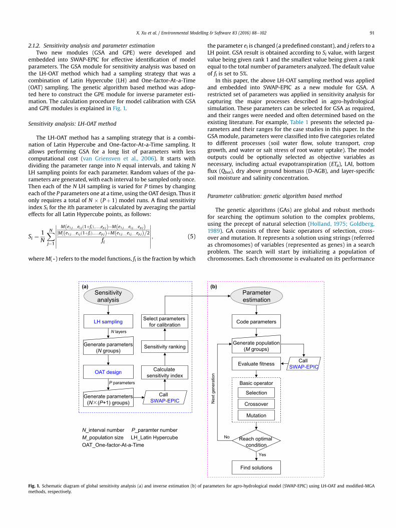
embedded into SWAP-EPIC for effective identification of modelparameters. The GSA module for sensitivity analysis was based onthe LH-OAT method which had a sampling strategy that was acombination of Latin Hypercube (LH) and One-factor-At-a-Time(OAT) sampling. The genetic algorithm based method was adop-ted here to construct the GPE module for inverse parameter esti-mation. The calculation procedure for model calibration with GSAand GPE modules is explained in Fig. 1.

Sensitivity analysis: LH-OAT method

The LH-OAT method has a sampling strategy that is a combi-nation of Latin Hypercube and One-factor-At-a-Time sampling. Itallows performing GSA for a long list of parameters with lesscomputational cost (van Griensven et al., 2006). It starts withdividing the parameter range into N equal intervals, and taking NLH sampling points for each parameter. Random values of the pa-rameters are generated, with each interval to be sampled only once.Then each of the N LH sampling is varied for P times by changingeach of the P parameters one at a time, using the OAT design. Thus itonly requires a total of N � (Pþ 1) model runs. A final sensitivityindex Si for the ith parameter is calculated by averaging the partialeffects for all Latin Hypercube points, as follows:

Si ¼1N

XNj¼1

Mðe1;j;…;ei;jð1þfiÞ;…;ep;jÞ�Mðe1;j;…;ei;j;…;ep;jÞ

½M�ðe1;j;…;ei;jð1þfiÞ;…;ep;jÞþMðe1;j;…;ei;j;…;ep;jÞ=2fi

; (5)

whereM(∙) refers to the model functions, fi is the fraction by which

Fig. 1. Schematic diagram of global sensitivity analysis (a) and inverse estimation (b) of pamethods, respectively.

the parameter ei is changed (a predefined constant), and j refers to aLH point. GSA result is obtained according to Si value, with largestvalue being given rank 1 and the smallest value being given a rankequal to the total number of parameters analyzed. The default valueof fi is set to 5%.

In this paper, the above LH-OAT sampling method was appliedand embedded into SWAP-EPIC as a new module for GSA. Arestricted set of parameters was applied in sensitivity analysis forcapturing the major processes described in agro-hydrologicalsimulation. These parameters can be selected for GSA as required,and their ranges were needed and often determined based on theexisting literature. For example, Table 1 presents the selected pa-rameters and their ranges for the case studies in this paper. In theGSA module, parameters were classified into five categories relatedto different processes (soil water flow, solute transport, cropgrowth, and water or salt stress of root water uptake). The modeloutputs could be optionally selected as objective variables asnecessary, including actual evapotranspiration (ETa), LAI, bottomflux (Qbot), dry above ground biomass (D-AGB), and layer-specificsoil moisture and salinity concentration.

Parameter calibration: genetic algorithm based method

The genetic algorithms (GAs) are global and robust methodsfor searching the optimum solution to the complex problems,using the precept of natural selection (Holland, 1975; Goldberg,1989). GA consists of three basic operators of selection, cross-over and mutation. It represents a solution using strings (referredas chromosomes) of variables (represented as genes) in a searchproblem. The search will start by initializing a population ofchromosomes. Each chromosome is evaluated on its performance

rameters for agro-hydrological model (SWAP-EPIC) using LH-OAT and modified-MGA

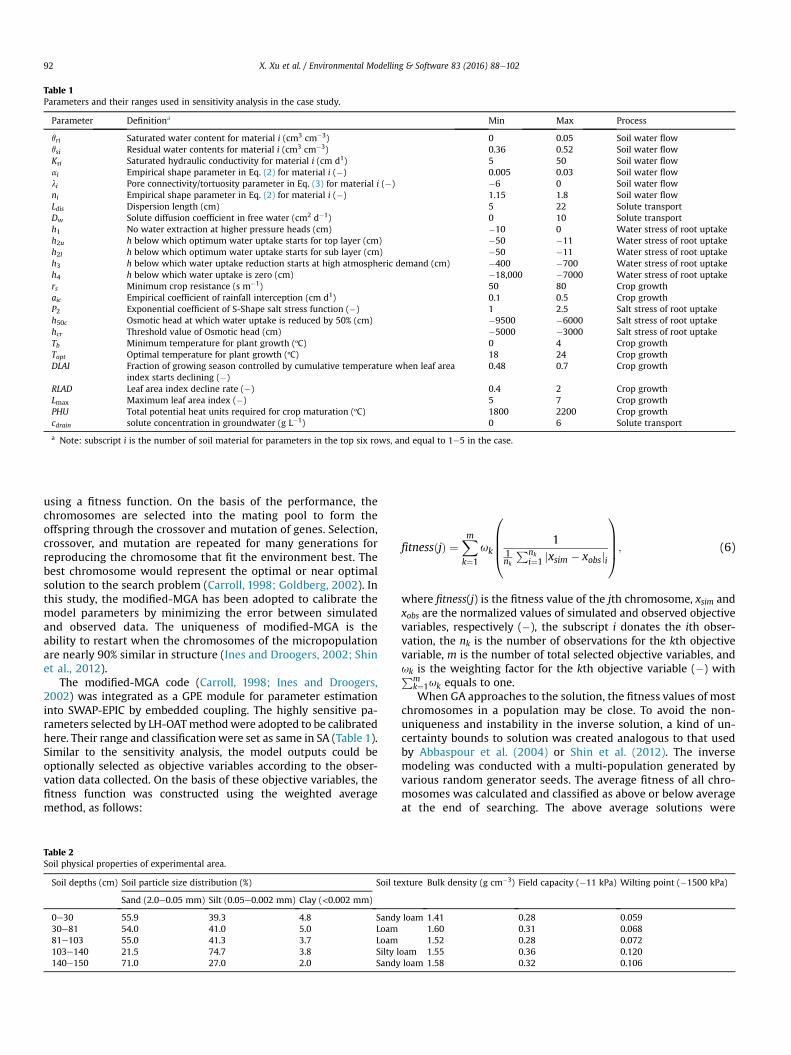
Table 1Parameters and their ranges used in sensitivity analysis in the case study.

Parameter Definitiona Min Max Process

qri Saturated water content for material i (cm3 cm�3) 0 0.05 Soil water flowqsi Residual water contents for material i (cm3 cm�3) 0.36 0.52 Soil water flowKsi Saturated hydraulic conductivity for material i (cm d1) 5 50 Soil water flowai Empirical shape parameter in Eq. (2) for material i (�) 0.005 0.03 Soil water flowli Pore connectivity/tortuosity parameter in Eq. (3) for material i (�) �6 0 Soil water flowni Empirical shape parameter in Eq. (2) for material i (�) 1.15 1.8 Soil water flowLdis Dispersion length (cm) 5 22 Solute transportDw Solute diffusion coefficient in free water (cm2 d�1) 0 10 Solute transporth1 No water extraction at higher pressure heads (cm) �10 0 Water stress of root uptakeh2u h below which optimum water uptake starts for top layer (cm) �50 �11 Water stress of root uptakeh2l h below which optimum water uptake starts for sub layer (cm) �50 �11 Water stress of root uptakeh3 h below which water uptake reduction starts at high atmospheric demand (cm) �400 �700 Water stress of root uptakeh4 h below which water uptake is zero (cm) �18,000 �7000 Water stress of root uptakers Minimum crop resistance (s m�1) 50 80 Crop growthaic Empirical coefficient of rainfall interception (cm d1) 0.1 0.5 Crop growthP2 Exponential coefficient of S-Shape salt stress function (�) 1 2.5 Salt stress of root uptakeh50c Osmotic head at which water uptake is reduced by 50% (cm) �9500 �6000 Salt stress of root uptakehcr Threshold value of Osmotic head (cm) �5000 �3000 Salt stress of root uptakeTb Minimum temperature for plant growth (ºC) 0 4 Crop growthTopt Optimal temperature for plant growth (ºC) 18 24 Crop growthDLAI Fraction of growing season controlled by cumulative temperature when leaf area

index starts declining (�)0.48 0.7 Crop growth

RLAD Leaf area index decline rate (�) 0.4 2 Crop growthLmax Maximum leaf area index (�) 5 7 Crop growthPHU Total potential heat units required for crop maturation (ºC) 1800 2200 Crop growthcdrain solute concentration in groundwater (g L�1) 0 6 Solute transport

a Note: subscript i is the number of soil material for parameters in the top six rows, and equal to 1e5 in the case.

X. Xu et al. / Environmental Modelling & Software 83 (2016) 88e10292

using a fitness function. On the basis of the performance, thechromosomes are selected into the mating pool to form theoffspring through the crossover and mutation of genes. Selection,crossover, and mutation are repeated for many generations forreproducing the chromosome that fit the environment best. Thebest chromosome would represent the optimal or near optimalsolution to the search problem (Carroll, 1998; Goldberg, 2002). Inthis study, the modified-MGA has been adopted to calibrate themodel parameters by minimizing the error between simulatedand observed data. The uniqueness of modified-MGA is theability to restart when the chromosomes of the micropopulationare nearly 90% similar in structure (Ines and Droogers, 2002; Shinet al., 2012).

The modified-MGA code (Carroll, 1998; Ines and Droogers,2002) was integrated as a GPE module for parameter estimationinto SWAP-EPIC by embedded coupling. The highly sensitive pa-rameters selected by LH-OATmethodwere adopted to be calibratedhere. Their range and classificationwere set as same in SA (Table 1).Similar to the sensitivity analysis, the model outputs could beoptionally selected as objective variables according to the obser-vation data collected. On the basis of these objective variables, thefitness function was constructed using the weighted averagemethod, as follows:

Table 2Soil physical properties of experimental area.

Soil depths (cm) Soil particle size distribution (%) Soil te

Sand (2.0e0.05 mm) Silt (0.05e0.002 mm) Clay (<0.002 mm)

0e30 55.9 39.3 4.8 Sandy30e81 54.0 41.0 5.0 Loam81e103 55.0 41.3 3.7 Loam103e140 21.5 74.7 3.8 Silty l140e150 71.0 27.0 2.0 Sandy

fitnessðjÞ ¼Xmk¼1

uk

0BBB@ 1

1nk

Pnki¼1 jxsim � xobsji

1CCCA; (6)

where fitness(j) is the fitness value of the jth chromosome, xsim andxobs are the normalized values of simulated and observed objectivevariables, respectively (�), the subscript i donates the ith obser-vation, the nk is the number of observations for the kth objectivevariable, m is the number of total selected objective variables, anduk is the weighting factor for the kth objective variable (�) withPm

k¼1uk equals to one.When GA approaches to the solution, the fitness values of most

chromosomes in a population may be close. To avoid the non-uniqueness and instability in the inverse solution, a kind of un-certainty bounds to solution was created analogous to that usedby Abbaspour et al. (2004) or Shin et al. (2012). The inversemodeling was conducted with a multi-population generated byvarious random generator seeds. The average fitness of all chro-mosomes was calculated and classified as above or below averageat the end of searching. The above average solutions were

xture Bulk density (g cm�3) Field capacity (�11 kPa) Wilting point (�1500 kPa)

loam 1.41 0.28 0.0591.60 0.31 0.0681.52 0.28 0.072

oam 1.55 0.36 0.120loam 1.58 0.32 0.106

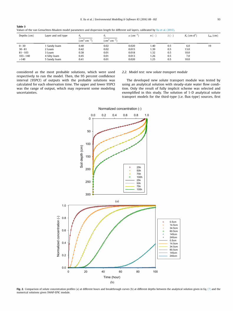
Table 3Values of the van Genuchten-Mualem model parameters and dispersion length for different soil layers, calibrated by Xu et al. (2013).

Depths (cm) Layer and soil type qs qr a (cm�1) n (�) l (�) Ks (cm d1) Ldis (cm)

(cm3 cm�3) (cm3 cm�3)

0e30 1 Sandy loam 0.40 0.02 0.020 1.40 0.5 6.0 1930e81 2 Loam 0.42 0.02 0.015 1.39 0.5 13.081e103 3 Loam 0.38 0.01 0.018 1.32 0.5 10.0103e140 4 Silty loam 0.45 0.01 0.013 1.26 0.5 7.0>140 5 Sandy loam 0.41 0.01 0.020 1.25 0.5 10.0

X. Xu et al. / Environmental Modelling & Software 83 (2016) 88e102 93

considered as the most probable solutions, which were usedrespectively to run the model. Then, the 95 percent confidenceinterval (95PCI) of outputs with the probable solutions wascalculated for each observation time. The upper and lower 95PCIwas the range of output, which may represent some modelinguncertainties.

Fig. 2. Comparison of solute concentration profiles (a) at different hours and breakthroughnumerical solutions given SWAP-EPIC module.

2.2. Model test: new solute transport module

The developed new solute transport module was tested byusing an analytical solution with steady-state water flow condi-tion. Only the result of fully implicit scheme was selected andexemplified in this study. The solution of 1-D analytical solutetransport models for the third-type (i.e. flux-type) sources, first

curves (b) at different depths between the analytical solution given in Eq. (7) and the

X. Xu et al. / Environmental Modelling & Software 83 (2016) 88e10294

obtained by Lindstrom et al. (1967), is used and presented asfollows (Batu, 2005):

Cnðz; tÞ ¼ C � CiC0 � Ci

¼ 12erfc

"Rdz� Ut

2ðDRdtÞ1=2

#þ�

U2tpDRd

�1=2

exp

"� ðRdz� UtÞ2

4DRdt

#

� 12

�1þ Uz

Dþ U2tDRd

�exp

�UzD

�erfc

Rdzþ Ut

2ðDRdtÞ1=2

!;

(7)

where Cn(z, t) is the normalized concentration, Ci and C0 arerespectively the initial and boundary flux concentration (g L�1), Rdis the solute retardation factor (�), D is the effective dispersioncoefficient (cm2 d�1), U is the average pore-water velocity (cm d1).The governing differential equation and related initial and

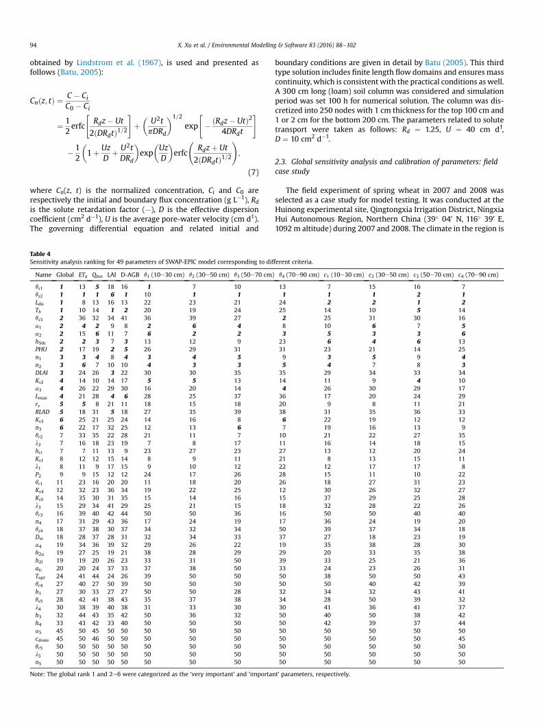
Table 4Sensitivity analysis ranking for 49 parameters of SWAP-EPIC model corresponding to dif

Name Global ETa Qbot LAI D-AGB q1 (10e30 cm) q2 (30e50 cm) q3 (50e70 cm)

qs1 1 13 5 18 16 1 7 10qs2 1 1 1 6 1 10 1 1Ldis 1 8 13 16 13 22 23 21Tb 1 10 14 1 2 20 19 24qs3 2 36 32 34 41 36 39 27a1 2 4 2 9 8 2 6 4a2 2 15 6 11 7 6 2 2h50c 2 2 3 7 3 13 12 9PHU 2 17 19 2 5 26 29 31n1 3 3 4 8 4 3 4 5n2 3 6 7 10 10 4 3 3DLAI 3 24 26 3 22 30 30 35Ks2 4 14 10 14 17 5 5 13a3 4 26 22 29 30 16 20 14Lmax 4 21 28 4 6 28 25 37rs 5 5 8 21 11 18 15 18RLAD 5 18 31 5 18 27 35 39Ks3 6 25 21 25 24 14 16 8n3 6 22 17 32 25 12 13 6qr2 7 33 35 22 28 21 11 7l2 7 16 18 23 19 7 8 17hcr 7 7 11 13 9 23 27 23Ks1 8 12 12 15 14 8 9 11l1 8 11 9 17 15 9 10 12P2 9 9 15 12 12 24 17 26qr1 11 23 16 20 20 11 18 20Ks4 12 32 23 36 34 19 22 25Ks5 14 35 30 31 35 15 14 16l3 15 29 34 41 29 25 21 15qr3 16 39 40 42 44 50 50 36n4 17 31 29 43 36 17 24 19qs4 18 37 38 30 37 34 32 34Dw 18 28 37 28 31 32 34 33a4 19 34 36 39 32 29 26 22h2u 19 27 25 19 21 38 28 29h2l 19 19 20 26 23 33 31 50aic 20 20 24 37 33 37 38 50Topt 24 41 44 24 26 39 50 50qr4 27 40 27 50 39 50 50 50h1 27 30 33 27 27 50 50 28qs5 28 42 41 38 43 35 37 38l4 30 38 39 40 38 31 33 30h3 32 44 43 35 42 50 36 32h4 33 43 42 33 40 50 50 50a5 45 50 45 50 50 50 50 50cdrain 45 50 46 50 50 50 50 50qr5 50 50 50 50 50 50 50 50l5 50 50 50 50 50 50 50 50n5 50 50 50 50 50 50 50 50

Note: The global rank 1 and 2e6 were categorized as the ‘very important’ and ‘importan

boundary conditions are given in detail by Batu (2005). This thirdtype solution includes finite length flow domains and ensures masscontinuity, which is consistent with the practical conditions as well.A 300 cm long (loam) soil column was considered and simulationperiod was set 100 h for numerical solution. The column was dis-cretized into 250 nodes with 1 cm thickness for the top 100 cm and1 or 2 cm for the bottom 200 cm. The parameters related to solutetransport were taken as follows: Rd ¼ 1.25, U ¼ 40 cm d1,D ¼ 10 cm2 d�1.

2.3. Global sensitivity analysis and calibration of parameters: fieldcase study

The field experiment of spring wheat in 2007 and 2008 wasselected as a case study for model testing. It was conducted at theHuinong experimental site, Qingtongxia Irrigation District, NingxiaHui Autonomous Region, Northern China (39� 040 N, 116� 39’ E,1092m altitude) during 2007 and 2008. The climate in the region is

ferent criteria.

q4 (70e90 cm) c1 (10e30 cm) c2 (30e50 cm) c3 (50e70 cm) c4 (70e90 cm)

13 7 15 16 71 1 1 2 1

24 2 2 1 225 14 10 5 142 25 31 30 168 10 6 7 53 5 3 3 6

23 6 4 6 1331 23 21 14 259 3 5 9 45 4 7 8 3

35 29 34 33 3414 11 9 4 104 26 30 29 17

36 17 20 24 2920 9 8 11 2138 31 35 36 336 22 19 12 127 19 16 13 9

10 21 22 27 3511 16 14 18 1527 13 12 20 2421 8 13 15 1122 12 17 17 828 15 11 10 2226 18 27 31 2312 30 26 32 2715 37 29 25 2818 32 28 22 2616 50 50 40 4017 36 24 19 2050 39 37 34 1837 27 18 23 1919 35 38 28 3029 20 33 35 3839 33 25 21 3633 24 23 26 3150 38 50 50 4350 50 40 42 3932 34 32 43 4134 28 50 39 3230 41 36 41 3750 40 50 38 4250 42 39 37 4450 50 50 50 5050 50 50 50 4550 50 50 50 5050 50 50 50 5050 50 50 50 50

t’ parameters, respectively.

X. Xu et al. / Environmental Modelling & Software 83 (2016) 88e102 95

arid continental and during the experimental period the averageannual rainfall is 194 mm, with more than 70% of precipitationoccurring between June and September. The experiment data hadbeen used to calibrate the previous version of SWAP-EPIC by Xuet al. (2013) that presented a detail description of experimentconditions. The information related to weather, soil properties,groundwater, irrigation, cultivation practices, and observationswere provided in Xu et al. (2013). Table 2 provides the main soilphysical properties of the studied soil with five layers.

A soil profile with 300 cm depth was specified during simula-tions. It was divided into five horizon layers up to 150 cm, according

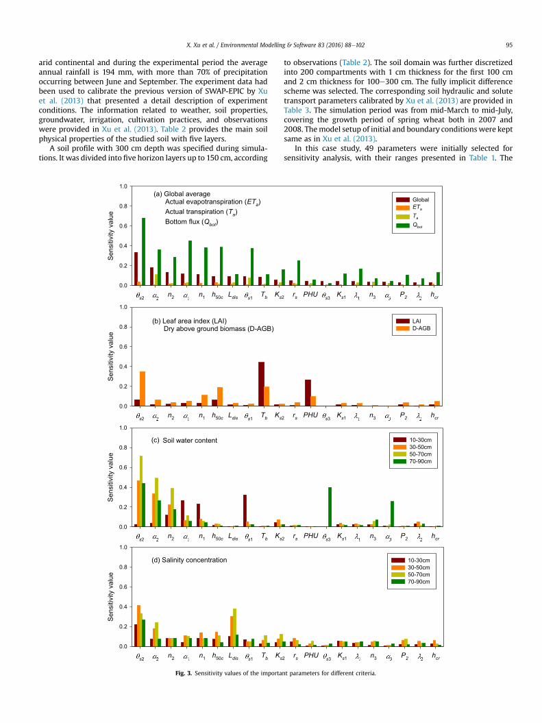
Fig. 3. Sensitivity values of the importa

to observations (Table 2). The soil domain was further discretizedinto 200 compartments with 1 cm thickness for the first 100 cmand 2 cm thickness for 100e300 cm. The fully implicit differencescheme was selected. The corresponding soil hydraulic and solutetransport parameters calibrated by Xu et al. (2013) are provided inTable 3. The simulation period was from mid-March to mid-July,covering the growth period of spring wheat both in 2007 and2008. Themodel setup of initial and boundary conditions were keptsame as in Xu et al. (2013).

In this case study, 49 parameters were initially selected forsensitivity analysis, with their ranges presented in Table 1. The

nt parameters for different criteria.

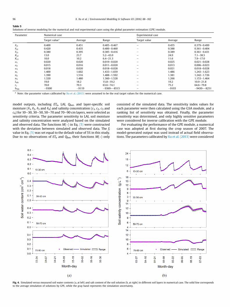
Table 5Solutions of inverse modeling for the numerical and real experimental cases using the global parameter estimation (GPE) module.

Parameter Numerical case Experimental case

Target valuea Average Range Target value Average Range

qs1 0.400 0.451 0.405e0.467 e 0.455 0.379e0.499qs2 0.420 0.435 0.400e0.460 e 0.388 0.361e0.404qs3 0.380 0.395 0.385e0.416 e 0.389 0.361e0.431Ks2 13.0 23.7 5.2e43.0 e 24.9 7.1e38.5Ks3 10.0 10.2 6.4e21.3 e 11.6 7.9e17.0a1 0.020 0.020 0.019e0.020 e 0.025 0.021e0.028a2 0.015 0.016 0.011e0.020 e 0.013 0.006e0.023a3 0.018 0.020 0.018e0.028 e 0.021 0.018e0.028n1 1.400 1.602 1.433e1.659 e 1.486 1.243e1.623n2 1.390 1.516 1.488e1.592 e 1.381 1.242e1.726n3 1.320 1.480 1.360e1.528 e 1.266 1.153e1.464Ldis 19.0 18.2 15.8e19.2 e 19.2 10.9e21.8rs 70.0 70.3 63.6e74.1 e 75.2 64.6e79.8h50c �9300 �9119 �9369~e8515 e �9103 �9430~e8251

a Note: the parameter values calibrated by Xu et al. (2013) were assumed to be the real target values for the numerical case.

X. Xu et al. / Environmental Modelling & Software 83 (2016) 88e10296

model outputs, including ETa, LAI, Qbot, and layer-specific soilmoisture (q1, q2, q3 and q4) and salinity concentration (c1, c2, c3 andc4) for 10e30, 30e50, 50e70 and 70e90 cm layers, were selected assensitivity criteria. The parameter sensitivity to LAI, soil moistureand salinity concentration were analyzed based on the simulatedand observed data. The functions M(∙) in Eq. (5) were constructedwith the deviation between simulated and observed data. The fivalue in Eq. (5) was set equal to the default value of 5% in this study.Due to no observations of ETa and Qbot, their functions M(∙) only

Fig. 4. Simulated versus measured soil water contents (a, at left) and salt content of the soilto the average simulation of solutions by GPE, while the gray band represents the simulati

consisted of the simulated data. The sensitivity index values foreach parameter were then calculated using the GSA module, and aranking list of sensitivity was obtained. Finally, the parametersensitivity was determined, and only highly sensitive parameterswere considered for inverse calibration with the GPE module.

For evaluating the performance of the GPE module, a numericalcase was adopted at first during the crop season of 2007. Themodel-generated output was used instead of actual field observa-tions. The parameters calibrated by Xu et al. (2013) were considered

solution (b, at right) in different soil layers in numerical case. The solid line correspondson uncertainty.

X. Xu et al. / Environmental Modelling & Software 83 (2016) 88e102 97

for this numerical case as the real parameter values (Table 3).Running the SWAP-EPIC model with the above parameters, and thegenerated output was assumed as the “measured” values in theinverse modeling. The daily measured (hypothetical) ETa, layer-specific soil moisture (q1, q2, q3 and q4) and salinity concentration(c1, c2, c3 and c4) were used to construct the fitness function (Eq.(6)). The weighting factor was respectively set to 0.20, 0.50 and0.30. ETa was selected as an objective because it has become aroutine observation by various methods (e.g. lysimeter, eddycovariance and remote sensing).

Next, the real field measurements were used to test the appli-cability of GPE module (i.e. the experimental case). The fitnessfunction for the experimental case was composed by the observedLAI, layer-specific soil moisture, and salinity concentration. Theweighted factor was the same as in the numerical case with LAIinstead of ETa. The parameters were firstly calibrated though in-verse modeling using the experimental data in 2007 season. Thenthe inverse parameters were also validated by using the observeddata in 2008 season.

The mean relative error (MRE), the root mean square error(RMSE), the Nash and Sutcliffe model efficiency (NSE), the coeffi-cient of determination (R2) were used to quantify the model fittingperformance. These indicators were defined as follows:

MRE ¼ 1N

XNi¼1

ðPi � OiÞOi

� 100%; (8)

RMSE ¼ffiffiffiffiffiffiffiffiffiffiffiffiffiffiffiffiffiffiffiffiffiffiffiffiffiffiffiffiffiffiffiffiffiffi1N

XNi¼1

ðPi � OiÞ2vuut ; (9)

NSE ¼ 1�PN

i¼1ðPi � OiÞ2PNi¼1

�Oi � O

2 ; (10)

R2 ¼

266664

PNi¼1

�Oi � O

�Pi � P

�ffiffiffiffiffiffiffiffiffiffiffiffiffiffiffiffiffiffiffiffiffiffiffiffiffiffiffiffiffiffiffiffiffiffiffiffiffiffiffiffiffiffiffiffiffiffiffiffiffiffiffiffiffiffiffiffiffiffiffiffiffiffiffiffiffiffiPN

i¼1

�Oi � O

2PNi¼1�Pi � P

�2r377775

2

; (11)

where N is the total number of observations, Pi and Oi are respec-tively the ith model simulated and observed values (i ¼ 1, 2, …, N),and P and O are the simulated and observed mean values, respec-tively. NSE ¼ 1.0 represents a perfect fit, and negative NSE valuesindicate that the mean observed value is a better predictor than thesimulated value (Moriasi et al., 2007). Note that when calculatingthe above indicators, the simulated value (Pi) corresponded to theaverage of simulation results obtained by all probable solutions,both for the numerical and experimental cases.

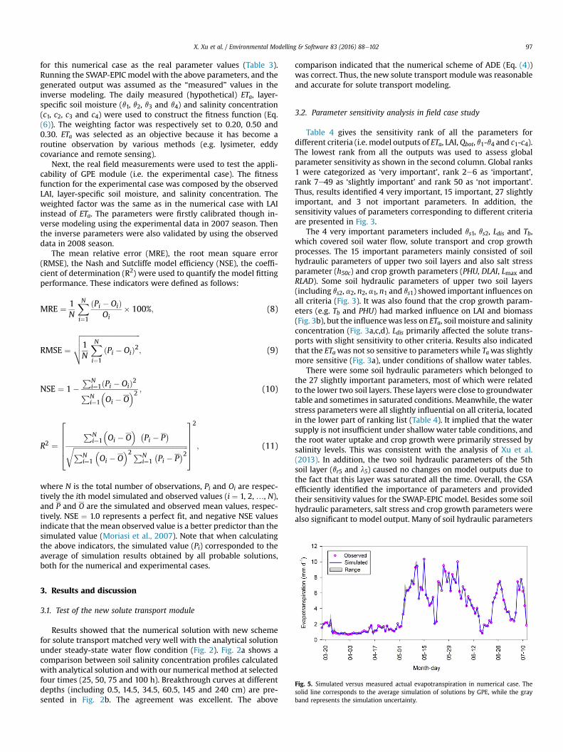
Fig. 5. Simulated versus measured actual evapotranspiration in numerical case. Thesolid line corresponds to the average simulation of solutions by GPE, while the grayband represents the simulation uncertainty.

3. Results and discussion

3.1. Test of the new solute transport module

Results showed that the numerical solution with new schemefor solute transport matched very well with the analytical solutionunder steady-state water flow condition (Fig. 2). Fig. 2a shows acomparison between soil salinity concentration profiles calculatedwith analytical solution and with our numerical method at selectedfour times (25, 50, 75 and 100 h). Breakthrough curves at differentdepths (including 0.5, 14.5, 34.5, 60.5, 145 and 240 cm) are pre-sented in Fig. 2b. The agreement was excellent. The above

comparison indicated that the numerical scheme of ADE (Eq. (4))was correct. Thus, the new solute transport module was reasonableand accurate for solute transport modeling.

3.2. Parameter sensitivity analysis in field case study

Table 4 gives the sensitivity rank of all the parameters fordifferent criteria (i.e. model outputs of ETa, LAI, Qbot, q1-q4 and c1-c4).The lowest rank from all the outputs was used to assess globalparameter sensitivity as shown in the second column. Global ranks1 were categorized as ‘very important’, rank 2e6 as ‘important’,rank 7e49 as ‘slightly important’ and rank 50 as ‘not important’.Thus, results identified 4 very important, 15 important, 27 slightlyimportant, and 3 not important parameters. In addition, thesensitivity values of parameters corresponding to different criteriaare presented in Fig. 3.

The 4 very important parameters included qs1, qs2, Ldis and Tb,which covered soil water flow, solute transport and crop growthprocesses. The 15 important parameters mainly consisted of soilhydraulic parameters of upper two soil layers and also salt stressparameter (h50c) and crop growth parameters (PHU, DLAI, Lmax andRLAD). Some soil hydraulic parameters of upper two soil layers(including qs2, a2, n2, a1, n1 and qs1) showed important influences onall criteria (Fig. 3). It was also found that the crop growth param-eters (e.g. Tb and PHU) had marked influence on LAI and biomass(Fig. 3b), but the influencewas less on ETa, soil moisture and salinityconcentration (Fig. 3a,c,d). Ldis primarily affected the solute trans-ports with slight sensitivity to other criteria. Results also indicatedthat the ETawas not so sensitive to parameters while Tawas slightlymore sensitive (Fig. 3a), under conditions of shallow water tables.

There were some soil hydraulic parameters which belonged tothe 27 slightly important parameters, most of which were relatedto the lower two soil layers. These layers were close to groundwatertable and sometimes in saturated conditions. Meanwhile, the waterstress parameters were all slightly influential on all criteria, locatedin the lower part of ranking list (Table 4). It implied that the watersupply is not insufficient under shallow water table conditions, andthe root water uptake and crop growth were primarily stressed bysalinity levels. This was consistent with the analysis of Xu et al.(2013). In addition, the two soil hydraulic parameters of the 5thsoil layer (qr5 and l5) caused no changes on model outputs due tothe fact that this layer was saturated all the time. Overall, the GSAefficiently identified the importance of parameters and providedtheir sensitivity values for the SWAP-EPIC model. Besides some soilhydraulic parameters, salt stress and crop growth parameters werealso significant to model output. Many of soil hydraulic parameters

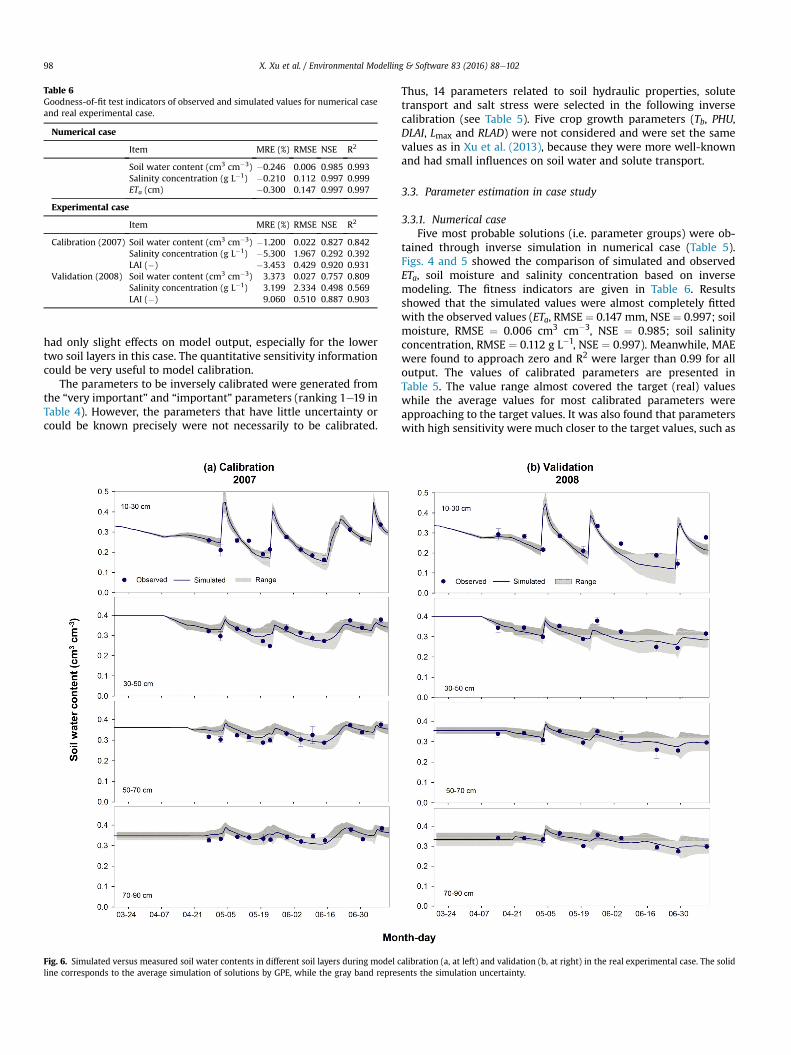
Table 6Goodness-of-fit test indicators of observed and simulated values for numerical caseand real experimental case.

Numerical case

Item MRE (%) RMSE NSE R2

Soil water content (cm3 cm�3) �0.246 0.006 0.985 0.993Salinity concentration (g L�1) �0.210 0.112 0.997 0.999ETa (cm) �0.300 0.147 0.997 0.997

Experimental case

Item MRE (%) RMSE NSE R2

Calibration (2007) Soil water content (cm3 cm�3) �1.200 0.022 0.827 0.842Salinity concentration (g L�1) �5.300 1.967 0.292 0.392LAI (�) �3.453 0.429 0.920 0.931

Validation (2008) Soil water content (cm3 cm�3) 3.373 0.027 0.757 0.809Salinity concentration (g L�1) 3.199 2.334 0.498 0.569LAI (�) 9.060 0.510 0.887 0.903

X. Xu et al. / Environmental Modelling & Software 83 (2016) 88e10298

had only slight effects on model output, especially for the lowertwo soil layers in this case. The quantitative sensitivity informationcould be very useful to model calibration.

The parameters to be inversely calibrated were generated fromthe “very important” and “important” parameters (ranking 1e19 inTable 4). However, the parameters that have little uncertainty orcould be known precisely were not necessarily to be calibrated.

Fig. 6. Simulated versus measured soil water contents in different soil layers during model cline corresponds to the average simulation of solutions by GPE, while the gray band repres

Thus, 14 parameters related to soil hydraulic properties, solutetransport and salt stress were selected in the following inversecalibration (see Table 5). Five crop growth parameters (Tb, PHU,DLAI, Lmax and RLAD) were not considered and were set the samevalues as in Xu et al. (2013), because they were more well-knownand had small influences on soil water and solute transport.

3.3. Parameter estimation in case study

3.3.1. Numerical caseFive most probable solutions (i.e. parameter groups) were ob-

tained through inverse simulation in numerical case (Table 5).Figs. 4 and 5 showed the comparison of simulated and observedETa, soil moisture and salinity concentration based on inversemodeling. The fitness indicators are given in Table 6. Resultsshowed that the simulated values were almost completely fittedwith the observed values (ETa, RMSE ¼ 0.147 mm, NSE ¼ 0.997; soilmoisture, RMSE ¼ 0.006 cm3 cm�3, NSE ¼ 0.985; soil salinityconcentration, RMSE ¼ 0.112 g L�1, NSE ¼ 0.997). Meanwhile, MAEwere found to approach zero and R2 were larger than 0.99 for alloutput. The values of calibrated parameters are presented inTable 5. The value range almost covered the target (real) valueswhile the average values for most calibrated parameters wereapproaching to the target values. It was also found that parameterswith high sensitivity were much closer to the target values, such as

alibration (a, at left) and validation (b, at right) in the real experimental case. The solidents the simulation uncertainty.

X. Xu et al. / Environmental Modelling & Software 83 (2016) 88e102 99

a1, a2 and Ldis. However, the parameter range might also have animpact on the accuracy of inverse estimation. For example, theaccuracy of inverse estimation for the most important parametersqs2 was not the highest. Some parameters were more uncertain anddifficult to estimate such as Ks2 that had relatively low sensitivity.The uncertainty bound for simulated ETa, soil moisture and salinityconcentration is presented in Figs. 4 and 5, respectively. There werevery small uncertainties for all model output. In summary, theestimated and targeted values for 14 selected parameters were veryclose with each other, and the simulated data matched very wellwith observed daily data with some small uncertainties. Thus, thenumerical case showed that the GPE module had a potential abilityfor inverse parameter estimation for agro-hydrological model.

3.3.2. Experimental caseEight probable solutions were obtained by inverse calibration

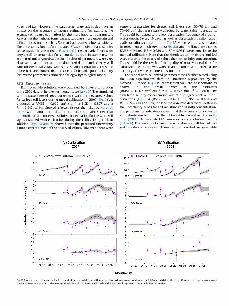
using 2007 data in field experimental case (Table 5). The simulatedsoil moisture showed good agreement with the measured valuesfor various soil layers during model calibration in 2007 (Fig. 6a). Itproduced a RMSE ¼ 0.022 cm3 cm�3, a NSE ¼ 0.827 and aR2 ¼ 0.842, which showed a better fitness than that by Xu et al.(2013) with manual try-and-error method. Fig. 7a also shows thatthe simulated and observed salinity concentration for the same soillayers matched with each other during the calibration period. Inaddition, Figs. 6a and 7a showed that the predicted uncertaintybounds covered most of the observed values. However, there were

Fig. 7. Simulated versus measured salt content of the soil solution in different soil layers duThe solid line corresponds to the average simulation of solutions by GPE, while the gray ba

some discrepancies for deeper soil layers (i.e. 50e70 cm and70e90 cm) that were partly affected by water table fluctuations.This could be related to the low observation frequency of ground-water depths (every 10 days) as well as observation quality (espe-cially for salinity concentration). The LAI values were also simulatedin agreement with observations (Fig. 8a), and the fitness results (i.e.RMSE ¼ 0.429, NSE ¼ 0.920 and R2 ¼ 0.931) were superior to themanual calibration. Note that the simulated soil moisture and LAIwere closer to the observed values than soil salinity concentration.This should be the result of the quality of observational data forsalinity concentration was worse than the other two. It affected theaccuracy of inverse parameter estimation.

The model with calibrated parameters was further tested usingthe 2008 experimental data. Soil moisture reproduced by theSWAP-EPIC model (Fig. 6b) represented well the observations asshown in the small errors of the estimates(RMSE ¼ 0.027 cm3 cm�3, NSE ¼ 0.757 and R2 ¼ 0.809). Thesimulated salinity concentration was also in agreement with ob-servations (Fig. 7b) (RMSE ¼ 2.334 g L�1, NSC ¼ 0.498 andR2 ¼ 0.569). In addition, most of the observed data were located inthe uncertainty bands for soil moisture and salinity concentration.The performance indicators showed that the accuracy for soil waterand salinity was better than that obtained by manual method in Xuet al. (2013). The simulated LAI was also closer to observed values(Table 6). The uncertainty bound was relatively small for LAI andsoil salinity concentration. These results indicated an acceptably

ring model calibration (a, left) and validation (b, at right) in the real experimental case.nd represents the simulation uncertainty.

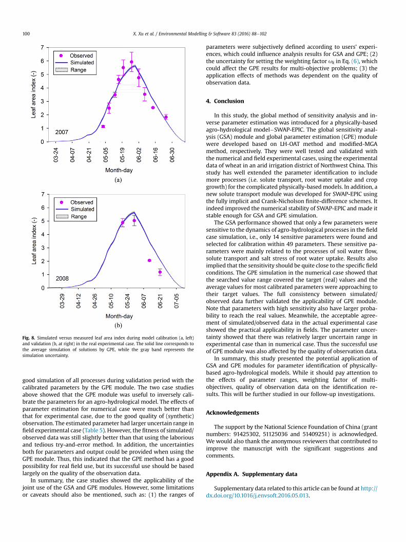
Fig. 8. Simulated versus measured leaf area index during model calibration (a, left)and validation (b, at right) in the real experimental case. The solid line corresponds tothe average simulation of solutions by GPE, while the gray band represents thesimulation uncertainty.

X. Xu et al. / Environmental Modelling & Software 83 (2016) 88e102100

good simulation of all processes during validation period with thecalibrated parameters by the GPE module. The two case studiesabove showed that the GPE module was useful to inversely cali-brate the parameters for an agro-hydrological model. The effects ofparameter estimation for numerical case were much better thanthat for experimental case, due to the good quality of (synthetic)observation. The estimated parameter had larger uncertain range infield experimental case (Table 5). However, the fitness of simulated/observed data was still slightly better than that using the laboriousand tedious try-and-error method. In addition, the uncertaintiesboth for parameters and output could be provided when using theGPE module. Thus, this indicated that the GPE method has a goodpossibility for real field use, but its successful use should be basedlargely on the quality of the observation data.

In summary, the case studies showed the applicability of thejoint use of the GSA and GPE modules. However, some limitationsor caveats should also be mentioned, such as: (1) the ranges of

parameters were subjectively defined according to users’ experi-ences, which could influence analysis results for GSA and GPE; (2)the uncertainty for setting the weighting factor uk in Eq. (6), whichcould affect the GPE results for multi-objective problems; (3) theapplication effects of methods was dependent on the quality ofobservation data.

4. Conclusion

In this study, the global method of sensitivity analysis and in-verse parameter estimation was introduced for a physically-basedagro-hydrological model�SWAP-EPIC. The global sensitivity anal-ysis (GSA) module and global parameter estimation (GPE) modulewere developed based on LH-OAT method and modified-MGAmethod, respectively. They were well tested and validated withthe numerical and field experimental cases, using the experimentaldata of wheat in an arid irrigation district of Northwest China. Thisstudy has well extended the parameter identification to includemore processes (i.e. solute transport, root water uptake and cropgrowth) for the complicated physically-basedmodels. In addition, anew solute transport module was developed for SWAP-EPIC usingthe fully implicit and Crank-Nicholson finite-difference schemes. Itindeed improved the numerical stability of SWAP-EPIC and made itstable enough for GSA and GPE simulation.

The GSA performance showed that only a few parameters weresensitive to the dynamics of agro-hydrological processes in the fieldcase simulation, i.e., only 14 sensitive parameters were found andselected for calibration within 49 parameters. These sensitive pa-rameters were mainly related to the processes of soil water flow,solute transport and salt stress of root water uptake. Results alsoimplied that the sensitivity should be quite close to the specific fieldconditions. The GPE simulation in the numerical case showed thatthe searched value range covered the target (real) values and theaverage values for most calibrated parameters were approaching totheir target values. The full consistency between simulated/observed data further validated the applicability of GPE module.Note that parameters with high sensitivity also have larger proba-bility to reach the real values. Meanwhile, the acceptable agree-ment of simulated/observed data in the actual experimental caseshowed the practical applicability in fields. The parameter uncer-tainty showed that there was relatively larger uncertain range inexperimental case than in numerical case. Thus the successful useof GPE module was also affected by the quality of observation data.

In summary, this study presented the potential application ofGSA and GPE modules for parameter identification of physically-based agro-hydrological models. While it should pay attention tothe effects of parameter ranges, weighting factor of multi-objectives, quality of observation data on the identification re-sults. This will be further studied in our follow-up investigations.

Acknowledgements

The support by the National Science Foundation of China (grantnumbers: 91425302, 51125036 and 51409251) is acknowledged.We would also thank the anonymous reviewers that contributed toimprove the manuscript with the significant suggestions andcomments.

Appendix A. Supplementary data

Supplementary data related to this article can be found at http://dx.doi.org/10.1016/j.envsoft.2016.05.013.

X. Xu et al. / Environmental Modelling & Software 83 (2016) 88e102 101

References

Abbaspour, K.C., Schulin, R., van Genuchten, M.T., 2001. Estimating unsaturated soilhydraulic parameters using ant colony optimization. Adv. Water Resour. 24 (8),827e841.

Abbaspour, K.C., Johnson, C.A., van Genuchten, M.T., 2004. Estimating uncertainflow and transport parameters using a sequential uncertainty fitting procedure.Vadose Zone J. 3 (4), 1340e1352.

Allen, R.G., Pereira, L.S., Raes, D., Smith, M., 1998. Guidelines for Computing CropWater Requirements. Crop evapotranspiration, FAO, Rome, Italy. Irrigation andDrainage Paper ¼56.

Batu, V., 2005. Applied Flow and Solute Transport Modeling in Aquifers: Funda-mental Principles and Analytical and Numerical Methods. CRC Press.

Black, T.A., Gardner, W.R., Thurtell, G.W., 1969. The prediction of evaporation,drainage, and soil water storage for a bare soil. Soil Sci. Soc. Am. J. 33 (5),655e660.

Boesten, J., Stroosnijder, L., 1986. Simple model for daily evaporation from fallowtilled soil under spring conditions in a temperate climate. Neth J. Agric. Sci. 34,75e90.

Boesten, J.J.T.I., van der Linden, A.M.A., 1991. Modeling the influence of sorption andtransformation on pesticide leaching and persistence. J. Environ. Qual. 20 (2),425e435.

Borg, H., Grimes, D.W., 1986. Depth development of roots with time: an empiricaldescription. Trans. ASAE 29 (1), 194e197.

Campolongo, F., Cariboni, J., Saltelli, A., 2007. An effective screening design forsensitivity analysis of large models. Environ. Modell. Softw. 22 (10), 1509e1518.

Cariboni, J., Gatelli, D., Liska, R., Saltelli, A., 2007. The role of sensitivity analysis inecological modeling. Ecol. Modell. 203 (1e2), 167e182.

Carroll, D.L., 1998. GA Fortran Driver Version 1.7 [EB/OL]. http://www.cuaerospace.com/carroll/ga.html.

DeJonge, K.C., Ascough II, J.C., Ahmadi, M., Andales, A.A., Arabi, M., 2012. Globalsensitivity and uncertainty analysis of a dynamic agroecosystem model underdifferent irrigation treatments. Ecol. Modell. 231, 113e125.

Della Peruta, R., Keller, A., Schulin, R., 2014. Sensitivity analysis, calibration andvalidation of EPIC for modelling soil phosphorus dynamics in Swiss agro-eco-systems. Environ. Modell. Softw. 62, 97e111.

Dirksen, C., Augustijn, D.C., 1988. Root Water Uptake Function for NonuniformPressure and Osmotic Potentials. ASA, Madison, WI, 185. Agronomy Abstract.

Duan, Q., Sorooshian, S., Gupta, V.K., 1994. Optimal use of the SCE-UA global opti-mization method for calibrating watershed models. J. Hydrol. 158 (3e4),265e284.

Easterling, W.E., Rosenberg, N.J., McKenney, M.S., Jones, C.A., Dyke, P.T.,Williams, J.R., 1992. Preparing the erosion productivity impact calculator (EPIC)model to simulate crop response to climate change and the direct effects of CO2.Agric. Meteorol. 59 (1e2), 17e34.

Evensen, G., 2003. The Ensemble Kalman filter: theoretical formulation and prac-tical implementation. Ocean. Dyn. 53 (4), 343e367.

Goldberg, D.E., 1989. Genetic Algorithms in Search, Optimization and MachineLearning. Addison-Wesley, Reading, Mass.

Goldberg, D.E., 2002. The Design of Innovation: Lessons from and for CompetentGenetic Algorithms. Springer Science & Business Media.

Hamby, D.M., 1994. A review of techniques for parameter sensitivity analysis ofenvironmental models. Environ. Monit. Assess. 32 (2), 135e154.

Holland, J.H., 1975. Adaptation in Natural and Artificial Systems, Edited. Universityof Michigan Press, Ann Arbor.

Hu, Y., Garcia-Cabrejo, O., Cai, X., Valocchi, A.J., DuPont, B., 2015. Global sensitivityanalysis for large-scale socio-hydrological models using Hadoop. Environ.Modell. Softw. 73, 231e243.

Hupet, F., Lambot, S., Feddes, R.A., van Dam, J.C., Vanclooster, M., 2003. Estimation ofroot water uptake parameters by inverse modeling with soil water contentdata. Water Resour. Res. 39 (11), 1312.

Ines, A.V., Mohanty, B.P., 2008. Near-surface soil moisture assimilation for quanti-fying effective soil hydraulic properties using genetic algorithm: 1. Conceptualmodeling. Water Resour. Res. 44, W06422. http://dx.doi.org/10.1029/2007WR005990.

Ines, A.V.M., Droogers, P., 2002. Inverse modelling in estimating soil hydraulicfunctions: a Genetic Algorithm approach. Hydrol. Earth Syst. Sci. 6 (1), 49e66.

Jacques, D., �Sim�unek, J., Timmerman, A., Feyen, J., 2002. Calibration of Richards' andconvectionedispersion equations to field-scale water flow and solute transportunder rainfall conditions. J. Hydrol. 259 (1e4), 15e31.

Jiang, Y., Xu, X., Huang, Q., Huo, Z., Huang, G., 2015. Assessment of irrigation per-formance and water productivity in irrigated areas of the middle Heihe Riverbasin using a distributed agro-hydrological model. Agric. Water Manage 147,67e81.

Jones, C.A., 1985. C4 Grasses and Cereals. John Wiley and Sons, Inc., New York,p. 412.

Kool, J.B., Parker, J.C., van Genuchten, M.T., 1987. Parameter estimation for unsatu-rated flow and transport modelsdA review. J. Hydrol. 91 (3e4), 255e293.

Kroes, J.G., van Dam, J.C., 2003. Reference Manual SWAP Version 3.0.3. Alterra,Green World Research, Wageningen, p. 211. Alterra-report 773.

Lindstrom, F.T., Haque, R., Freed, V.H., Boersma, L., 1967. The movement of someherbicides in soils. Linear diffusion and convection of chemicals in soils. Envi-ron. Sci. Technol. 1 (7), 561e565.

Malone, R.W., Jaynes, D.B., Ma, L., Nolan, B.T., Meek, D.W., Karlen, D.L., 2010. Soil-test

N recommendations augmented with PEST-optimized RZWQM simulations.J. Environ. Qual. 39 (5), 1711e1723.

Monsi, M., Saeki, T., 1953. Uber den Lictfaktor in den Pflanzengesellschaften undsein Bedeutung fur die Stoffproduktion. Jpn. J. Bot. 14, 22e52.

Monteith, J.L., 1965. Evaporation and the environment. In: The State and Movementof Water in Living Organisims. Cambridge University Press, Swansea,pp. 205e234.

Monteith, J.L., Moss, C.J., 1977. Climate and the efficiency of crop production inbritain [and discussion]. Philosophical transactions of the royal society ofLondon. B, Biol. Sci. 281 (980), 277e294.

Moriasi, D.N., Arnold, J.G., Van Liew, M.W., Bingner, R.L., Harmel, R.D., Veith, T.L.,2007. Model evaluation guidelines for systematic quantification of accuracy inwatershed simulations. Trans. ASABE 50 (3), 885e900.

Mualem, Y., 1976. A new model for predicting the hydraulic conductivity of un-saturated porous media. Water Resour. Res. 12 (3), 513e522.

Neelam, M., Mohanty, B.P., 2015. Global sensitivity analysis of the radiative transfermodel. Water Resour. Res. 51 (4), 2428e2443.

Nossent, J., Elsen, P., Bauwens, W., 2011. Sobol' sensitivity analysis of a complexenvironmental model. Environ. Modell. Softw. 26 (12), 1515e1525.

Paredes, P., Rodrigues, G.C., Alves, I., Pereira, L.S., 2014. Partitioning evapotranspi-ration, yield prediction and economic returns of maize under various irrigationmanagement strategies. Agric. Water Manage 135, 27e39.

Pianosi, F., Sarrazin, F., Wagener, T.A., 2015. Matlab toolbox for global sensitivityanalysis. Environ. Modell. Softw. 70, 80e85.

Ranatunga, K., Nation, E.R., Barratt, D.G., 2008. Review of soil water models andtheir applications in Australia. Environ. Modell. Softw. 23 (9), 1182e1206.

Saltelli, A., Tarantola, S., Chan, K., 1999. A quantitative model-independent methodfor global sensitivity analysis of model output. Technometrics 41 (1), 39e56.

Saltelli, A., Annoni, P., 2010. How to avoid a perfunctory sensitivity analysis. Environ.Modell. Softw. 25 (12), 1508e1517.

Sarrazin, F., Pianosi, F., Wagener, T., 2016. Global sensitivity analysis of environ-mental models: convergence and validation. Environ. Modell. Softw. 79,135e152.

Shafiei, M., Ghahraman, B., Saghafian, B., Davary, K., Pande, S., Vazifedoust, M., 2014.Uncertainty assessment of the agro-hydrological SWAP model application atfield scale: a case study in a dry region. Agric. Water Manage 146, 324e334.

Shin, Y., Mohanty, B.P., Ines, A.V.M., 2012. Soil hydraulic properties in one-dimensional layered soil profile using layer-specific soil moisture assimilationscheme. Water Resour. Res. 48, W06529. http://dx.doi.org/10.1029/2010WR009581.

�Sim�unek, J., van Genuchten, M.T., 1996. Estimating unsaturated soil hydraulicproperties from tension disc infiltrometer data by numerical inversion. WaterResour. Res. 32 (9), 2683e2696.

�Sim�unek, J., Huang, K., van Genuchten, M.T., 1997. The HYDRUS-et software packagefor simulating the one-dimensional movement of water, heat and multiplesolutes in variably-saturated media. In: Bratislava: Inst. Hydrology, Slovak Acad.Sci, p. 184. Version 1.1.

Stockle, C.O., Williams, J.R., Rosenberg, N.J., Jones, C.A., 1992. A method for esti-mating the direct and climatic effects of rising atmospheric carbon dioxide ongrowth and yield of crops: Part IdModification of the EPIC model for climatechange analysis. Agric. Syst. 38 (3), 225e238.

van Dam, J.C., Huygen, J., Wesseling, J.G., Feddes, R.A., Kabat, P., van Walsum, P.E.V.,Groenendijk, P., van Diepen, C.A., 1997. Theory of SWAP Version 2.0. Simulationof Water Flow, Solute Transport and Plant Growth in theSoilewatereatmosphereeplant Environment. DLOWinand Staring Centre-DLO,p. 167. Department of water resources, WAU, Report 71, technical Document 45.

van Dam, J.C., Groenendijk, P., Hendriks, R.F.A., Kroes, J.G., 2008. Advances ofmodeling water flow in variably saturated soils with SWAP. Vadose Zone J. 7 (2),640e653.

van Genuchten, M.T., Wierenga, P.J., 1974. Simulation of One-dimensional SoluteTransfer in Porous Media. New Mexico Agricultural Experiment Station Bulletin628, Las Cruces, N.M.

van Genuchten, M.T., 1980. A closed-form equation for predicting the hydraulicconductivity of unsaturated soils. Soil Sci. Soc. Am. J. 44 (5), 892e898.

van Griensven, A., Meixner, T., Grunwald, S., Bishop, T., Diluzio, M., Srinivasan, R.,2006. A global sensitivity analysis tool for the parameters of multi-variablecatchment models. J. Hydrol. 324 (1e4), 10e23.

Varella, H., Gu�erif, M., Buis, S., 2010. Global sensitivity analysis measures the qualityof parameter estimation: the case of soil parameters and a crop model. Environ.Modell. Softw. 25 (3), 310e319.

Wesseling, J.G., Kroes, J.G., Metselaar, K., 1998. Global Sensitivity Analysis of theSoil-water-atmosphere-plant (SWAP) Model. DLO-Staring Centre, p. 70. Report160.

Williams, J.R., Jones, C.A., Kiniry, J.R., Spanel, D.A., 1989. The EPIC crop growthmodel. Trans. ASAE 32 (2), 497e511.

W€ohling, T., Vrugt, J.A., Barkle, G.F., 2008. Comparison of three multiobjectiveoptimization algorithms for inverse modeling of vadose zone hydraulic prop-erties. Soil Sci. Soc. Am. J. 72 (2), 305e319.

Xu, X., Qu, Z., Huang, G., 2012. Optimization of soil hydraulic and solute transportparameters using genetic algorithms at field scale. Shuili Xuebao J. Hydraul.Eng. 43 (7), 808e815.

Xu, X., Huang, G., Sun, C., Pereira, L.S., Ramos, T.B., Huang, Q., Hao, Y., 2013. Assessingthe effects of water table depth on water use, soil salinity and wheat yield:searching for a target depth for irrigated areas in the upper Yellow River basin.Agric. Water Manage 125, 46e60.

X. Xu et al. / Environmental Modelling & Software 83 (2016) 88e102102

Xu, X., Sun, C., Qu, Z., Huang, Q., Ramos, T.B., Huang, G., 2015. Groundwater rechargeand capillary rise in irrigated areas of the upper Yellow River basin assessed byan agro-Hydrological model. Irrig. Drain. http://dx.doi.org/10.1002/ird.1928.

Yang, J., 2011. Convergence and uncertainty analyses in Monte-Carlo based sensi-tivity analysis. Environ. Modell. Softw. 26 (4), 444e457.

Yang, J., Reichert, P., Abbaspour, K.C., Xia, J., Yang, H., 2008. Comparing uncertaintyanalysis techniques for a SWAT application to the Chaohe Basin in China.

J. Hydrol. 358 (1), 1e23.Zhao, G., Bryan, B.A., Song, X., 2014. Sensitivity and uncertainty analysis of the

APSIM-wheat model: interactions between cultivar, environmental, and man-agement parameters. Ecol. Modell. 279, 1e11.

Zheng, C., Bennett, G.D., 2002. Applied Contaminant Transport Modeling. Wiley-Interscience, New York.