ready or not: predicting high and low levels of school
TRANSCRIPT

1
WORKING PAPER
Ready or Not: Predicting High and Low Levels of School Readiness among Teenage Parents’ Children Stefanie Mollborn Jeff A. Dennis August 2010 Health and Society Program HS2010-02 ____________________________________________________________________________
1
Ready or Not: Predicting High and Low Levels of School Readiness among Teenage
Parents’ Children*
Stefanie Mollborn
University of Colorado at Boulder
Jeff A. Dennis
University of Texas of the Permian Basin
RUNNING HEAD: School Readiness among Teenage Parents’ Children
WORD COUNT: 7,326 (main text)
* This research is based on work supported by a grant from the Department of Health and Human Services,
Office of Public Health Service (#1 APRPA006015-01-00). The authors thank Professor Richard Jessor and
Casey Blalock for their contributions to this project. Direct correspondence to Stefanie Mollborn, Sociology
and Institute of Behavioral Science, 483 UCB, Boulder, CO 80309-0483. E-mail: [email protected].
2
Abstract
Past research has documented compromised development for teenage mothers’ children
compared to others, but less is known about predictors of school readiness among these children or
about teenage fathers’ children. Using parent interviews and direct assessments from the Early
Childhood Longitudinal Study-Birth Cohort, we identify factors associated with unusually high and
low math, reading, and behavior scores, and unusually good or bad health, shortly before
kindergarten. The sizeable sample of children born to a teenage mother and/or father facilitates the
inclusion of factors from five structural and interpersonal domains based on the School Transition
Model. Multinomial logistic regression models predict the likelihood of scoring in the highest, and
lowest, quintile compared to the middle quintile for math, reading, and behavior. Excellent, and
poor/fair/good, health are compared to very good health. Many children of teenage parents score
highly in one or more domains. The models strongly predict which children have unusually high or
low math and reading scores, and to a lesser degree behavior and health. Both relational and
structural factors are important for predicting variation in preschool outcomes among teenage
parents’ children. Important predictors differ depending on the domain being considered. Most
significant factors matter either for predicting unusually high or low scores, but not both. Policies
that improve families’ socioeconomic status and financial stability, as well as those that encourage
low-conflict, positive relationships and coresidence with fathers and grandparents, seem promising.
Encouraging relationship stability at any cost is not likely to benefit these children.
3
Ready or Not: Predicting High and Low Levels of School Readiness among Teenage Parents’ Children
Teenage childbearing is common in the United States today, with 18% of all girls expected to
give birth before age 20 (Perper & Manlove, 2009). After a long decline, the teenage birth rate has
stalled (Hamilton, Martin, & Ventura, 2010). Decades of research has addressed this issue, including
both its causes and its consequences for young parents and their children. Much of the research on
the consequences of teenage parenthood for children has compared the children of teenage mothers
to other children (e.g., Geronimus, Korenman, & Hillemeier, 1994; Levine, Pollack, & Comfort,
2001; Mollborn & Dennis, 2009; Moore & Snyder, 1991; Turley, 2003), while a smaller body of work
has focused on understanding differences in outcomes among children of teenage parents (Dubow &
Luster, 1990; Furstenberg, Brooks-Gunn, & Morgan, 1987a; Hubbs-Tait, Osofsky, Hann, & Culp,
1994; Luster, Bates, Fitzgerald, Vandenbelt, & Key, 2000; Luster, Lekskul, & Oh, 2004b). Asking
why some preschool-aged children of teenage parents end up well prepared to start school and
others do not is an important question with clear policy implications. This study uses data from the
Early Childhood Longitudinal Study-Birth Cohort to identify children who are likely to be at risk at
the start of the transition to school, as well as those who are likely to be quite successful. By
understanding social structural and interpersonal factors associated with belonging in one of these
groups, policymakers can better understand which children to target for interventions and which
factors have potential for protecting them.
This study focuses on three domains of child development that have been shown to be
important for children’s successful transitions to school and long-term outcomes (Entwisle,
Alexander, & Olson, 2004; Halonen, Aunola, Ahonen, & Nurmi, 2006; Weller, Schnittjer, & Tuten,
1992): academic preparedness, behavior, and health. They are all critical components of success in
the transition to school, which determines a large part of children’s academic outcomes throughout

4
compulsory schooling (Baydar, Brooks-Gunn, & Furstenberg, 1993). Health and education in
childhood work hand in hand to influence socioeconomic attainment and health in adulthood (Haas,
2007; Hayward & Gorman, 2004; Palloni, 2006; Ross & Wu, 1996). Crosnoe (2006) has identified
children’s health as a key component of the transition to school.
From past research, we know that on average, children of teenage mothers approach the
start of school at a disadvantage on each of these three dimensions (Geronimus et al., 1994; Levine
et al., 2001; Mollborn & Dennis, 2009; Moore & Snyder, 1991; Turley, 2003). Some research on the
causes of this disadvantage pinpoints preexisting factors, while other work identifies factors directly
related to early childbearing. Much less is known about children of teenage fathers, though several of
their preschool outcomes are also compromised (Mollborn & Dennis, 2009). But what factors are
associated with children doing unusually well or unusually poorly? This question requires a different
kind of approach than a typical mean-based regression analysis. Using a relatively large subsample of
children of teenage mothers and fathers on the cusp of the school transition (4½ years old), we
compare high-scoring and low-scoring children to those near the median on each dimension of
development. Previous studies each examine part of the puzzle in understanding variation in the
preschool outcomes of teenage mothers’ children, but none include children of teenage fathers, and
all use older or local data sources. We located one study that has compared unusually high- and low-
scoring preschool-aged children of teenage mothers (Luster et al., 2000). Although it explored a
variety of potential predictors in a nuanced, multi-method analysis, Luster and colleagues’ study was
based on a small (N=44) local sample, did not differentiate processes related to scoring particularly
low versus particularly high, and did not examine child outcomes beyond vocabulary scores.
THEORETICAL FRAMEWORK
In general, the preschool period is critical for children’s futures (Chase-Lansdale, Gordon,
Brooks-Gunn, & Klebanov, 1997; Mulligan & Flanagan, 2006). Cognitive, verbal, and behavioral
5
outcomes from early childhood predict success when children start school (Baydar et al., 1993). In
turn, children who start off doing well in elementary school tend to do better on later assessments of
achievement, are more likely to complete high school, and attain higher levels of education than
those who struggle at first (for a review, see Entwisle et al., 2004). Early language development has
important influences on later reading, spelling, and language, and its influence remains stable
throughout the first years of elementary school (Walker, Greenwood, Hart, & Carta, 1994) and for
years afterwards (Baydar et al., 1993). For all of these reasons, children’s readiness for the transition
to school is critical, laying the groundwork for long-term socioeconomic and health inequalities (see
Entwisle et al., 2004 for a review).
A variety of studies have shown that the children of teenage parents are at risk for
compromised development and health (Geronimus et al., 1994; Levine et al., 2001; Moore & Snyder,
1991; Turley, 2003). Teenagers are still developing psychologically and may not have the maturity
that older parents have, so there may be disparities between teenagers’ and adults’ parenting styles
and skills, home environments, and emotional resources that have developmental implications for
their children (Furstenberg, Brooks-Gunn, & Chase-Lansdale, 1989). Adolescents are more likely
than adults to engage in risky behaviors such as smoking, binge drinking, and delinquency that may
endanger their children as well as themselves (Jessor, Donovan, & Costa, 1991). Teenage parents are
also tackling the difficult task of parenting at the same time that they are working to build human
capital by completing schooling or starting a career, which may put them at risk of being less
successful in both these domains. They are in a life phase when many adolescents enter into and
terminate relationships with various partners as they gain experience with intimacy, potentially
resulting in higher levels of partner instability that can negatively affect their children (Fomby &
Cherlin, 2007; Osborne & McLanahan, 2007). These explanations deal with average differences
between teenagers and older parents, but it is easy to imagine that teenage parents differ in the

6
degree to which these factors are present and negatively impact their children. Indeed, Vandenbelt,
Luster, and Bates (2001) found that differences among low-income teenage mothers in home
environments and parenting at age 4 predicted children’s achievement in first grade.
The School Transition Model (Alexander, Entwisle, Blyth, & McAdoo, 1988; further articulated
by Crosnoe, 2006) provides a useful theoretical framework for organizing a variety of influences on
children’s school preparedness. In this model, children’s social structural circumstances, such as
socioeconomic resources, influence three sets of more proximate factors: social psychological factors
(interpersonal relationships), experiential factors (experiences outside of family relationships), and
personal factors (children’s attributes such as personality). All of these factors influence children’s
cognitive achievement in the transition to school. We extend the model to encompass health and
behavior. Crosnoe (2006) found that social structural factors influenced children’s health, which in
turn affected cognitive achievement. The same is true for behavior: Behavior problems indicate
compromised social and/or emotional development, and such problems in early childhood are
highly correlated with behavior problems and academic problems at school age (Halonen et al.,
2006). While the School Transition Model predicts children’s outcomes at the start of school, our
study assesses them shortly before, at age 4½. Luster, Lekskul, and Oh (2004b) found that children’s
language scores at this age predicted achievement test scores and teachers’ assessments of children’s
academic motivation in first grade.
One of the benefits of the School Transition Model is that it considers both structural and
relational factors to be important for understanding children’s chances of success. Although many
studies focus on one of these dimensions at the expense of the other, there is empirical support for
taking a broader perspective. For example, Jaffee and colleagues (2001) found in a sample of New
Zealanders that family circumstances and maternal characteristics mattered about equally for
predicting the long-term outcomes of children of teenage mothers. Oxford and Spieker (2006)
7
found in a local convenience sample that maternal characteristics interacted with the home
environment to influence children’s preschool language scores.
HYPOTHESES
Our hypotheses group potential influences on the reading and math scores, behavior, and
health of teenage parents’ children into categories, linking them with various facets of the School
Transition Model. Social structural hypotheses are followed by more proximate influences that the
model expects to be shaped by social structure. We cite past research justifying the inclusion of each
set of factors.
Hypothesis 1 (current socioeconomic resources): Children of teenage parents whose households have more
socioeconomic resources will be more likely to have positive health and developmental outcomes and less likely to have
negative outcomes. These are considered social structural factors in the School Transition Model.
Cooley and Unger (1991) used the National Longitudinal Survey of Youth, an older survey of
children born around 1980 and their mothers, to estimate the effects of “family factors,” including
several resource measures, on the academic and behavioral outcomes of teenage mothers’ children at
ages 6 to 7. They found that these resources had important positive associations with development.
In particular, family income is related to children’s cognitive outcomes and behavior problems at age
3 to 5 (see Yeung, Linver, & Brooks-Gunn, 2002 for a review). Income has been linked to children’s
intellectual development through cognitive stimulation in the home, parenting styles, the home’s
physical environment, and children’s health status at birth (Guo & Harris, 2000). Maternal education
is another socioeconomic resource that influences the development of teenage mothers’ children
(Cooley & Unger, 1991; Dubow & Luster, 1990; Luster et al., 2000; Luster, Bates, Vandenbelt, &
Nievar, 2004a). Extreme deprivation also matters for children’s development. For example,
experiencing hunger has been linked to compromised behavioral and cognitive development in
children (Kleinman et al., 1998).
8
Hypothesis 2 (maternal characteristics): Children of teenage parents whose mothers are working, enrolled in
school, have reached age 18, and have better mental health will be more likely to have positive outcomes and less likely
to have negative outcomes. In the School Transition Model, the first three of these factors fall into the
social structural category but have direct implications for children’s interactions with their mothers,
who are almost always the primary parent. Mothers’ mental health is considered a social
psychological factor. Luster and colleagues (2000) found that children whose teenage mothers
worked for pay were more likely to score very high than very low on vocabulary tests at age 4½. Past
research has also shown that younger teenage mothers and their children sometimes experience
worse outcomes than older teenage mothers (Hoffman, Foster, & Furstenberg, 1993; Levine et al.,
2001). Teenage mothers’ depression is another important predictor of young children’s behavior
(Black et al., 2002a; Hubbs-Tait et al., 1994) and cognitive outcomes (Rosman & Yoshikawa, 2001).
Hypothesis 3 (parenting): Children experiencing higher-quality parenting and home environments will be more
likely to have positive outcomes and less likely to have negative outcomes. These are considered social
psychological factors in the School Transition Model. The quality of teenage mothers’ parenting has
been linked to the language development of their children at ages 2½ (Luster & Vandenbelt, 1999)
and 4½ (Luster et al., 2000). The same two studies found home environment factors to be important
predictors, as did Oxford and Spieker (2006). A factor related to parenting, the attachment bond
between parent and child, has been associated with preschool behavior ratings by Hubbs-Tait
(1994).
Hypothesis 4 (parental relationships): Children of teenage parents whose mothers’ intimate relationships are
more stable and happier will be more likely to have positive outcomes and less likely to have negative outcomes. The
School Transition Model considers these to be social psychological factors. Both positive and
negative aspects of parent figures’ interactions have been found to be consequential for children’s
development. Black and colleagues (2002a) found that when teenage mothers assessed their partner

9
interactions more negatively, their children were more likely to experience externalizing behavior
problems at ages 4 to 5. Teenage mothers’ reports of relationship strain with their child’s father have
been associated with higher levels of their depression and anxiety (Gee & Rhodes, 2003), which are
linked to children’s outcomes above. Beyond the dynamics within the parent figures’ relationships,
their stability also matters for children. The repeated entry and exit of a parent’s romantic partners
from a child’s household has deleterious consequences for children’s development, including their
school readiness (Fomby & Cherlin, 2007; Osborne & McLanahan, 2007). Research on the effects of
union stability has rarely addressed the children of teen parents in particular, but Cooley and Unger
(1991) found that relationship stability was positively associated with the development of teenage
mothers’ children at 6 to 7 years old.
Hypothesis 5 (care provided by other adults): Children living with more adults and fewer other children and
those in child care are expected to interact more with adult caregivers and will therefore be more likely to have positive
outcomes and less likely to have negative outcomes. These are considered social psychological factors in the
School Transition Model, except for nonparental child care, which is an experiential factor because it
often occurs outside the family. Brooks-Gunn and Furstenberg (1986) reported that much of the
relationship between teenage motherhood and child outcomes was mediated by their higher
likelihood of living in single-parent households, which lack the resources that extra adults in the
household can provide. Although evidence is mixed, support from the child’s father has generally
been found to be beneficial for teenage mothers (Gee & Rhodes, 2003; see Roye & Balk, 1996 for a
review) and their children (Black et al., 2002a; Cooley & Unger, 1991; Coren, Barlow, & Stewart-
Brown, 2003; Luster et al., 2000). Living with parents potentially provides housing, child care, and
financial resources, and it improves teenage parents’ educational outcomes (Furstenberg &
Crawford, 1978; Trent & Harlan, 1994). Although some evidence is mixed (Black et al., 2002b), living
in a three-generation household with the child’s maternal grandmother is generally thought to be

10
beneficial for teenage mothers’ children’s development, at least early in the child’s life (Black et al.,
2002b; Pope et al., 1993). Even if a grandmother does not live with the child, her involvement in
child care in the child’s first couple of years is positive for development at age 6 to 7 (Cooley &
Unger, 1991). While additional adults may be beneficial for children, the presence of other children
can be problematic (Luster et al., 2000). More children means a greater need for resources of time,
money, and energy, and multiple teenage births have linked to greater levels of subsequent
disadvantage (Furstenberg, Brooks-Gunn, & Morgan, 1987b).
METHOD
Data
The Early Childhood Longitudinal Study-Birth Cohort (ECLS-B) selected a nationally
representative sample of about 14,000 children born in 2001 and followed families from infancy
through the start of kindergarten (U.S. Department of Education, 2007). It is the first U.S. nationally
representative survey to track children throughout this period of early life using parent interviews
and reputable direct assessments. The ECLS-B also includes unusually large numbers of children
with teenage mothers and fathers. The sample was drawn from births registered in the National
Center for Health Statistics vital statistics system based on a clustered, list frame sampling design.
Children were sampled from 96 core primary sampling units, which were counties and county
groups. Births to mothers younger than 15 were excluded for reasons of confidentiality and
sensitivity, so our findings are not representative of children with very young teenage mothers.
This study uses data from the first three waves of the survey, conducted when the children
were about 9, 24, and 52 months old. The primary parent, who almost always was the biological
mother, was interviewed in person. The weighted response rates for the parent interview were 74%,
93%, and 91% for Waves 1, 2, and 3. Stata software accounted for complex survey design using
replication weights that made findings representative of U.S. children born in 2001. The primary
11
analysis sample for this study was restricted to children who had at least one parent under age 20 at
their birth, whose biological mothers participated in the interview at all three waves, and who
completed child assessments at all three waves, resulting in about 950 eligible cases.1 After listwise
deletion of missing data, our main analysis samples for the various child outcomes ranged from
approximately 750 (for math and reading) to 800 (for behavior and health).2 Additional analyses for
specific hypotheses were restricted to: (1) cases that included direct parent assessments at Wave 2,
resulting in a sample of about 600 children for analyses of math scores, (2) children whose mothers
answered the mental health questions in the separate self-administered questionnaire (N≈700), and
(3) children whose mothers answered the questionnaire and were married or cohabiting at Wave 2
((N≈450).
Measures
Child preschool outcomes. We examined four measures of health and development at
Wave 3 (about age 4½), drawn from in-person child assessments and parent interviews (see Snow et
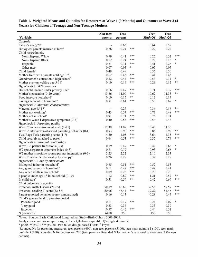
al., 2007 for more information). Table 1 presents descriptive information for all variables. Two
measures reflect direct assessments. Children’s reading scores were calculated based on a 35-item test
covering areas appropriate for pre-kindergarten learning such as phonological awareness, letter
sound knowledge, letter recognition, print conventions, and word recognition. Math scores were
calculated using a two-stage assessment routed after the first stage depending on the child’s score,
involving number sense, counting, operations, geometry, pattern understanding, and measurement.
1 Because of ECLS-B confidentiality requirements, all Ns are rounded to the nearest 50. We compared Wave 1 maternal education, poverty, and maternal age at birth for eligible cases to the 350 children of teenage parents who did not meet the eligibility requirements. The non-eligible cases exhibited 0.25 years lower Wave 1 maternal education (p<.05) but did not differ from eligible cases for maternal or paternal age or household poverty. 2 A substantial proportion of deleted cases were due to a lack of math and reading scores. Eligible children without math scores were compared to those with math scores on Wave 1 maternal characteristics, and the comparison indicates that children without math scores had mothers with less education at Wave 1 (p<.01) but had similar maternal ages and household poverty levels. Finally, we compared eligible children with math scores, but who were listwise deleted for other non-response, to the analysis sample. The listwise deleted children had mothers with significantly higher education at Wave 1 than those in the analysis sample (p<.001) and had a lower prevalence of being below the poverty line at Wave 1 (p<.01), but did not differ by maternal age.

12
Parent reports were the source of the two other measures. Children’s behavior is represented by a
standardized continuous variable, averaged from 24 items in which the parent was asked how
frequently the child exhibited specific behaviors, using a 5-point scale ranging from “never” to “very
often” (Cronbach alpha=0.86). For example, parents were asked how often the child shares
belongings or volunteers to help other children, how often the child is physically aggressive or acts
impulsively, and how well the child pays attention. Child health status was recoded into three
categories from the parent’s 5-category report, comparing very good to excellent and to
good/fair/poor. Small proportions of parents reporting child health in the three lower categories
necessitated combining them.
INSERT TABLE 1 ABOUT HERE
Current socioeconomic resources. All independent variables in this study were measured at
Wave 1 (9 months old) except where indicated. Our indicator of a household income below the
poverty line was calculated as an income-to-needs ratio using 2001 federal poverty guidelines, which
account for household size and income. In 14% of cases, household income was imputed by ECLS-
B using hot deck imputation. Maternal education was based on an ECLS-B constructed variable, with
highest degrees recoded into approximate years and logical adjustments made to correct
inconsistencies across waves. Household food security was constructed by ECLS-B, comparing food
secure to food insecure households. A final variable indicated whether someone in the household
had a checking or savings account.
Care provided by adults. Several variables measured the presence of potential caregivers in
the household, as well as other children who might reduce the amount of attention received from
adults. The biological father’s coresidence at Wave 1 was included as a dichotomous variable.
Dichotomous variables indicated whether any grandparent or any other adult, excluding parents or their
partners, lived in the household. Another variable counted the number of coresident children under
13
age 18 besides the study child. Finally, a dichotomous variable measured whether the study child
received any nonparental child care at Wave 1.
Maternal characteristics. Four variables measured characteristics of the child’s mother. An
indicator of very young maternal age was scored as 1 if the mother was under 18 at birth and 0
otherwise. Mothers’ paid work and school enrollment at Wave 1 were captured by dichotomous variables
for none versus any. Finally, mothers’ depressive symptoms were measured using a 12-item subset of
questions from the Center for Epidemiologic Studies-Distress Scale (CES-D; Radloff, 1977).
Mothers reported the frequency of experiencing specific symptoms in the last week, ranging from
never or rarely to most or all of the time. To retain cases with missing data on a few items, we
calculated the mean of available items, ranging from 0 to 3 (Cronbach alpha=0.87).
Parenting measures. Four measures captured aspects of the parent-child relationship and
the mother’s parenting at Wave 2 (age 2). Counts of positive versus negative or dangerous factors in
children’s home environments included 21 items ranging from the presence of books in the household,
to a consistent bedtime routine, to playing together. Interviewer-observed parenting behaviors during the
assessment counted mothers’ display of behaviors such as smacking, kissing/hugging, ensuring a
safe play environment, responding verbally to the child, and interfering with the child’s actions.
Eight items were coded as 0 for “negative” and 1 for “positive” parenting behaviors and averaged.
The Two Bags Task, a modification of the Three Bags Task used in prior research (Love et al., 2002),
is a videotaped problem-solving task in which parent and child played for 10 minutes with a set of
dishes and a picture book. For the parent score, coders rated mothers’ sensitivity, positive regard,
and stimulation of cognitive development of their child (Nord, Edwards, Andreassen, Green, &
Wallner-Allen, 2006). The Toddler Attachment Sort – 45, which modified the Attachment Q-Sort
(Nord et al., 2006), assessed the child’s attachment to the mother. Interviewers scored the child on

14
behaviors such as “seeks and enjoys being hugged” and “shows no fear, into everything.” The
child’s attachment relationship was coded as secure or not.
Mother’s marriage/cohabiting relationship. For all children in the sample, the number of
partner transitions experienced by the mother between Waves 1 and 3 was calculated. Based on
partners/spouses listed in the household roster at the time of each wave, this variable ranged from 0
to 3. The other measures were limited to children whose mothers completed the Wave 2 self-
administered questionnaire and who were married or cohabiting at Wave 2. An argument index was
created as the average of mothers’ reports that they and their coresident partner/spouse often,
sometimes, hardly ever, or never argued about 10 topics such as children, sex, and chores. A
measure of positive relationship interaction was calculated from mothers’ reports about how frequently
(ranging from less than once a month to almost every day) they and their coresident partner/spouse
talked about their days or their interests, laughed together, and calmly discussed things, worked
together on a project. Mothers’ relationship satisfaction with their spouse or coresident partner was
coded as 1 for “very happy” and 0 for “fairly happy” or “not too happy.”
Control variables. Demographic controls in this study’s multivariate analyses included the
child’s centered age in months at the Wave 3 assessment (which is necessary for correctly analyzing
the age-sensitive raw scores for math and reading, so it was included in all analyses that use these
raw scores), gender, and race/ethnicity (constructed by ECLS-B), the mother’s marital status at birth
(obtained from the birth certificate and coded as married versus other), and the father’s age at birth
(<20 years versus older). The ECLS-B survey also included maternal background factors that have
been found to influence both selection into teenage childbearing and its consequences (Oxford &
Spieker, 2006; SmithBattle, 2007): whether the mother’s household received welfare assistance
between ages 5 and 16, whether she lived with both parents until age 16, and her mother’s education
(less than a high school diploma versus higher).
15
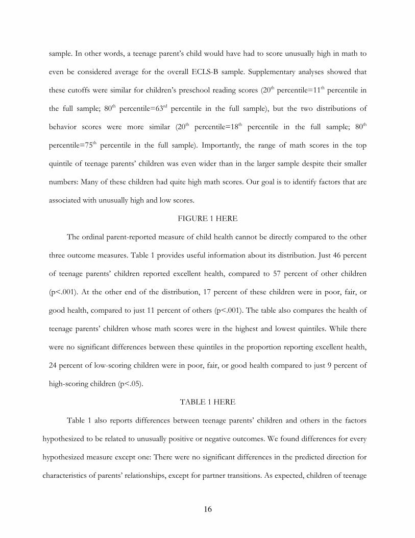
Analysis Plan
Rather than focusing on means as typical regression analyses do, this study predicted
particularly high or low scores on various measures of development and health. To this end, we
worked with quintiles of the distribution of math, reading, and behavior scores. Health was coded
into three categories (excellent, very good, and good/fair/poor) because of very small numbers of
parents reporting good, fair, and poor child health and a modal category of excellent. All analyses
were weighted to represent children born in the U.S. in 2001. Descriptive analyses display quintiles
of math scores for teenage parents’ children compared to all children, then compare children of
teenage parents who scored in the top versus the bottom quintile on math at Wave 3. Multinomial
logistic regression analyses compare children in the bottom quintile of math, reading, and behavior
to those in the middle quintile, as well as comparing the top quintile to the middle quintile. Using
similar logic, multivariate analyses of health compare good/fair/poor to very good and excellent to
very good. These multinomial logit models test our hypotheses. While our longitudinal data allowed
us to establish time order because the independent variables are measured years before the child
outcomes, the observational nature of the data did not permit us to establish causality.
RESULTS
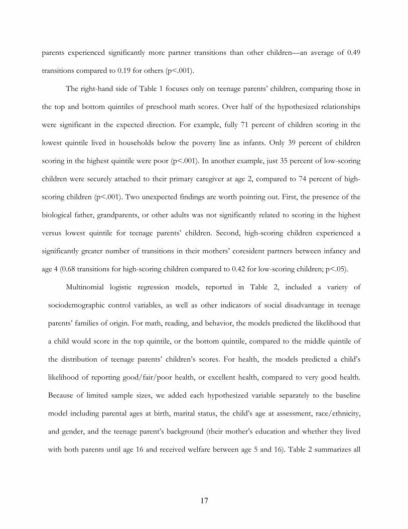
Descriptive analyses
Figure 1 displays the weighted quintile distribution of preschool (age 4) math scores for
children who had valid scores, comparing all children and for teenage parents’ children. The figure
shows that children in the bottom quintile had a wide range of scores, but the minimum score was
similar across the two groups. Teenage parents’ quintile cutoffs were lower than those of the full
sample. For example, the 20th percentile cutoff among teenage parents’ children fell below the 12th
percentile for the full sample. These differences accumulated across the distribution, resulting in the
80th percentile cutoff among teenage parents’ children falling below the 62nd percentile for the full
16
sample. In other words, a teenage parent’s child would have had to score unusually high in math to
even be considered average for the overall ECLS-B sample. Supplementary analyses showed that
these cutoffs were similar for children’s preschool reading scores (20th percentile=11th percentile in
the full sample; 80th percentile=63rd percentile in the full sample), but the two distributions of
behavior scores were more similar (20th percentile=18th percentile in the full sample; 80th
percentile=75th percentile in the full sample). Importantly, the range of math scores in the top
quintile of teenage parents’ children was even wider than in the larger sample despite their smaller
numbers: Many of these children had quite high math scores. Our goal is to identify factors that are
associated with unusually high and low scores.
FIGURE 1 HERE
The ordinal parent-reported measure of child health cannot be directly compared to the other
three outcome measures. Table 1 provides useful information about its distribution. Just 46 percent
of teenage parents’ children reported excellent health, compared to 57 percent of other children
(p<.001). At the other end of the distribution, 17 percent of these children were in poor, fair, or
good health, compared to just 11 percent of others (p<.001). The table also compares the health of
teenage parents’ children whose math scores were in the highest and lowest quintiles. While there
were no significant differences between these quintiles in the proportion reporting excellent health,
24 percent of low-scoring children were in poor, fair, or good health compared to just 9 percent of
high-scoring children (p<.05).
TABLE 1 HERE
Table 1 also reports differences between teenage parents’ children and others in the factors
hypothesized to be related to unusually positive or negative outcomes. We found differences for every
hypothesized measure except one: There were no significant differences in the predicted direction for
characteristics of parents’ relationships, except for partner transitions. As expected, children of teenage
17
parents experienced significantly more partner transitions than other children—an average of 0.49
transitions compared to 0.19 for others (p<.001).
The right-hand side of Table 1 focuses only on teenage parents’ children, comparing those in
the top and bottom quintiles of preschool math scores. Over half of the hypothesized relationships
were significant in the expected direction. For example, fully 71 percent of children scoring in the
lowest quintile lived in households below the poverty line as infants. Only 39 percent of children
scoring in the highest quintile were poor (p<.001). In another example, just 35 percent of low-scoring
children were securely attached to their primary caregiver at age 2, compared to 74 percent of high-
scoring children (p<.001). Two unexpected findings are worth pointing out. First, the presence of the
biological father, grandparents, or other adults was not significantly related to scoring in the highest
versus lowest quintile for teenage parents’ children. Second, high-scoring children experienced a
significantly greater number of transitions in their mothers’ coresident partners between infancy and
age 4 (0.68 transitions for high-scoring children compared to 0.42 for low-scoring children; p<.05).
Multinomial logistic regression models, reported in Table 2, included a variety of
sociodemographic control variables, as well as other indicators of social disadvantage in teenage
parents’ families of origin. For math, reading, and behavior, the models predicted the likelihood that
a child would score in the top quintile, or the bottom quintile, compared to the middle quintile of
the distribution of teenage parents’ children’s scores. For health, the models predicted a child’s
likelihood of reporting good/fair/poor health, or excellent health, compared to very good health.
Because of limited sample sizes, we added each hypothesized variable separately to the baseline
model including parental ages at birth, marital status, the child’s age at assessment, race/ethnicity,
and gender, and the teenage parent’s background (their mother’s education and whether they lived
with both parents until age 16 and received welfare between age 5 and 16). Table 2 summarizes all
18
significant results from this wide variety of models, highlighting findings that were significant in the
hypothesized direction.
TABLE 2 HERE
Children’s unusually high or low math scores were particularly strongly associated with the
variables in our models. Several relationships were significant in the hypothesized direction for
reading scores, compared to just a few relationships for behavior and health. More variables
significantly predicted children’s likelihood of scoring unusually high than unusually low. It is also
important to note that perhaps because of limited sample size, the significant relationships were
nearly all quite large in magnitude, suggesting that many variables we focused on are quite important
for understanding children’s outcomes. Eleven hypothesized factors predicted the likelihood that a
child would have unusually negative preschool outcomes, all in the hypothesized direction. These
significant relationships were split fairly evenly between math and reading, and fewer predicted
unusually low-scoring health. Fourteen factors predicted unusually positive outcomes, twelve in the
hypothesized direction. Two findings were significant in unexpected directions: the number of
partner transitions was positively associated with children’s likelihood of high-scoring behavior, and
young maternal age was positively related to children’s odds of excellent health (see below).
Seventeen of the 21 variables that we hypothesized would be related to children’s health and
development were indeed significant for one or more outcomes.
Each of the four socioeconomic resource variables addressed in Hypothesis 1 was associated
with at least one of the children’s outcomes (primarily math scores) as predicted. Children whose
household incomes were below the poverty line in infancy had a 116% higher likelihood than
nonpoor children of scoring in the bottom quintile in math at age 4.3 A one-year increase in maternal
education in infancy was associated with a 29% decrease in a child’s likelihood of scoring in the
3 Percentages and odds reported here and elsewhere come from odds ratios calculated by exponentiating the coefficients reported in Table 2.
19
bottom quintile in reading. Children from households that experienced food insecurity at Wave 1 had a
56% lower chance of scoring in the top quintile in math compared to those from food-secure
households. Children whose households had savings at Wave 1 were 110% more likely to score in the
top quintile for math, 52% less likely to score in the bottom quintile in reading, and 50% less likely
to score in the bottom quintile for behavior.
Each of the maternal characteristics addressed in Hypothesis 2 was related to children’s
outcomes as expected, except for mothers’ school enrollment. Young maternal age (15-17 years) was
associated with a 67% decrease in the likelihood of scoring in the top quintile for reading and a 64%
decrease for math. In an unexpected finding, children of the youngest mothers were 67% more likely
to report excellent compared to very good health than those with older teenage mothers. Children
whose mothers worked for pay at Wave 1 were 66% less likely to score in the bottom quintile in math.
Mothers who reported a higher level of depressive symptoms at Wave 1 were 51% less likely to score in
the top quintile for math and were 118% more likely to report that their child was in good, fair, or
poor health compared to very good health at age 4.
With the exception of the home environment measure, each of the parenting-related factors
from Hypothesis 3 was significantly associated with children’s outcomes as predicted. Moving from
the lowest to the highest possible score for interviewer-observed parenting behaviors at Wave 1 was
associated with 94% lower odds of the child scoring in the bottom quintile in reading. A one-point
increase in mothers’ Two Bags Task parenting scores at age 2 lowered children’s likelihood of scoring in
the bottom quintile on math at age 4 by 51%. Children who were securely attached to their primary
caregiver at age 2 were 344% more likely to score in the top quintile in math and 72% less likely to
score in the bottom quintile in reading.
The factors related to parents’ marriages/cohabiting relationships in Hypothesis 4 received more
limited support. Mothers’ happiness with their marriage/cohabiting relationship was not related to

20
children’s outcomes. In a finding that was actually significant in the opposite direction from the
hypothesis, each additional partner transition experienced by mothers between Waves 1 and 3 was
associated with a 79% higher likelihood of a child scoring in the top quintile for behavior. The other
two measures supported the hypothesis. More frequent arguments with the mother’s spouse or
cohabiting partner at age 2 were associated with a 57% lower likelihood of children scoring in the
top quintile for behavior at age 4 and a 75% greater likelihood of reporting the child as having good,
fair, or poor health compared to very good health. More frequent positive interactions between
spouses/partners at age 2 almost tripled a child’s odds of scoring in the top quintile for math at age 4.
Finally, most of the measures included in Hypothesis 5 were related to one or more of children’s
preschool outcomes as expected. Children who lived with their biological fathers as infants were over
2.5 times as likely to score in the top quintile in math at age 4 as those who did not. Those who lived
with at least one grandparent were twice as likely to score in the highest quintile in behavior. Each
additional child in the household was associated with a 28% lower likelihood of scoring in the top
quintile for math. Children of teenage parents who received nonparental child care as infants were
56% less likely to score in the bottom quintile for math than those without child care, and 173%
more likely to score in the top quintile in reading. The hypothesis was not supported for coresidence
with nonparent, nongrandparent adults.
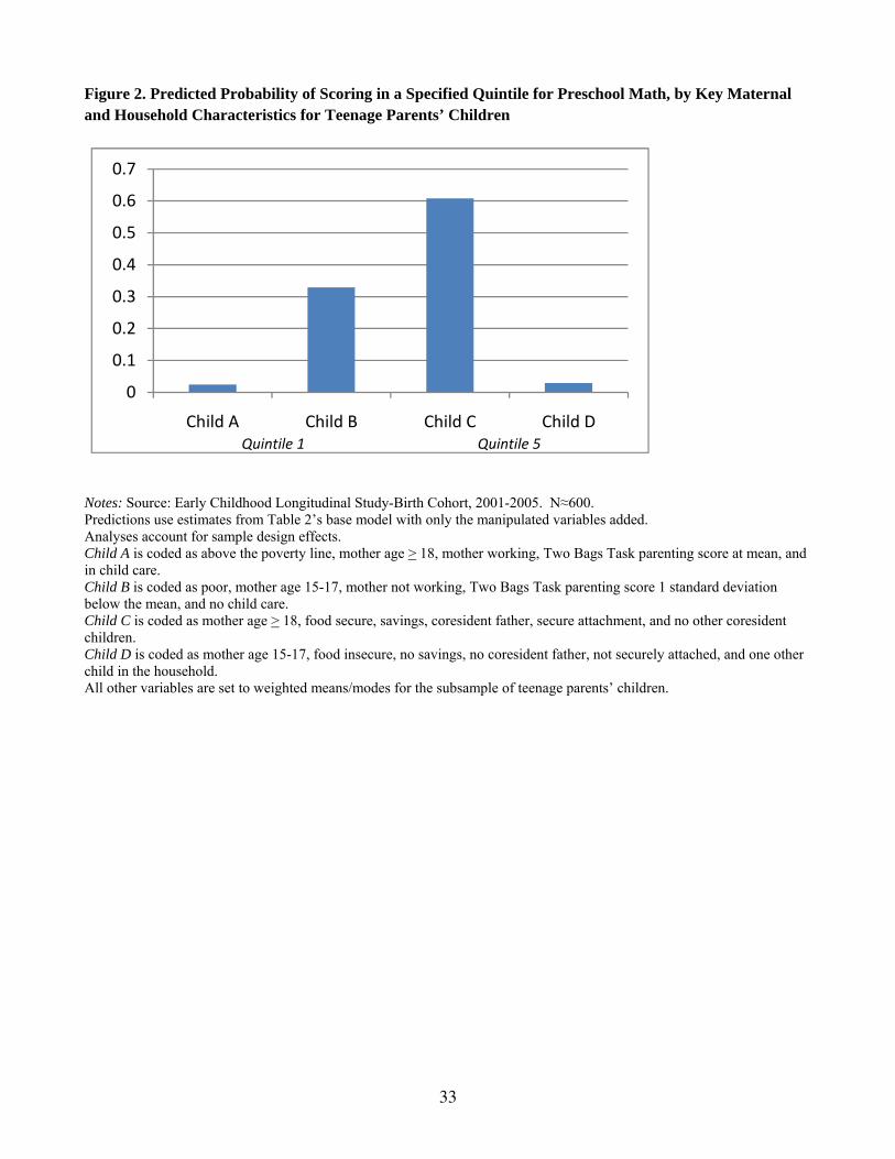
The importance of the factors we have identified for understanding a child’s preschool
outcomes can be illustrated using predicted probabilities of scoring in the top and bottom quintiles
for math. Using the parenting subsample to estimate models that include the baseline variables from
Table 2 and the hypothesized variables that are being manipulated for each pair, we compare
hypothetical children who have average (for continuous variables) or modal (for categorical
variables) values for the sample of teenage parents’ children on all variables except those we
manipulate (see Figure 2). The first comparison manipulates the factors that were found to predict
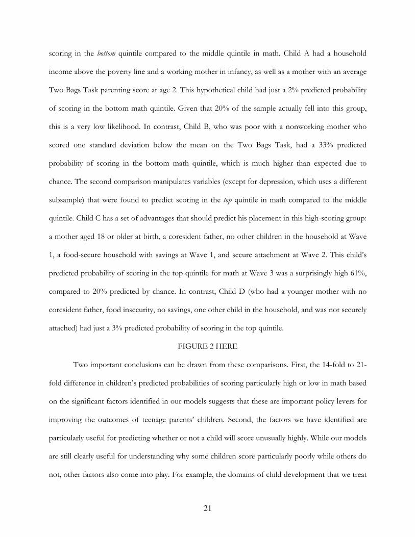
21
scoring in the bottom quintile compared to the middle quintile in math. Child A had a household
income above the poverty line and a working mother in infancy, as well as a mother with an average
Two Bags Task parenting score at age 2. This hypothetical child had just a 2% predicted probability
of scoring in the bottom math quintile. Given that 20% of the sample actually fell into this group,
this is a very low likelihood. In contrast, Child B, who was poor with a nonworking mother who
scored one standard deviation below the mean on the Two Bags Task, had a 33% predicted
probability of scoring in the bottom math quintile, which is much higher than expected due to
chance. The second comparison manipulates variables (except for depression, which uses a different
subsample) that were found to predict scoring in the top quintile in math compared to the middle
quintile. Child C has a set of advantages that should predict his placement in this high-scoring group:
a mother aged 18 or older at birth, a coresident father, no other children in the household at Wave
1, a food-secure household with savings at Wave 1, and secure attachment at Wave 2. This child’s
predicted probability of scoring in the top quintile for math at Wave 3 was a surprisingly high 61%,
compared to 20% predicted by chance. In contrast, Child D (who had a younger mother with no
coresident father, food insecurity, no savings, one other child in the household, and was not securely
attached) had just a 3% predicted probability of scoring in the top quintile.
FIGURE 2 HERE
Two important conclusions can be drawn from these comparisons. First, the 14-fold to 21-
fold difference in children’s predicted probabilities of scoring particularly high or low in math based
on the significant factors identified in our models suggests that these are important policy levers for
improving the outcomes of teenage parents’ children. Second, the factors we have identified are
particularly useful for predicting whether or not a child will score unusually highly. While our models
are still clearly useful for understanding why some children score particularly poorly while others do
not, other factors also come into play. For example, the domains of child development that we treat
22
as outcomes are intertwined and most often predict lower scores. Supplemental analyses show that
higher interviewer-observed behavior scores at age 2 predict a lower likelihood of scoring in the
bottom quintile for math and reading at age 4½.
DISCUSSION
The goal of this study was to identify factors associated with unusually positive or negative
health and development just prior to the start of kindergarten among children of teenage parents.
Grounded in the School Transition Model, our hypotheses suggested that socioeconomic resources,
care provided by adults, maternal characteristics such as age and depressive symptoms, parenting
quality, and parental relationship characteristics would all matter for these children’s outcomes. We
found that despite mean differences that disadvantaged teenage parents’ children compared to other
children for most of these factors in their first two years of life, many of these children scored quite
highly on math, reading, behavior, and health at age 4½. The hypothesized categories of factors
identified in this study did a good job predicting which children would score unusually poorly and a
better job predicting who would score unusually highly. Each of the five hypothesized domains was
important, and two measures (very young maternal age and household savings) were associated with
very high or low scores across three of the four outcomes we examined.
Several shortcomings of our study should be addressed in future research. First, confidentiality
restrictions precluded an investigation of children with mothers younger than 15, who are an
extremely small (Hamilton et al., 2010) but interesting population. Second, it would be useful to
understand the processes through which social structural and interpersonal factors are related to the
development and health of teenage parents’ children. Our ongoing quantitative and qualitative
research is working to address this question. Third, including more objective measures of behavior
and health in addition to parent reports would be an improvement. Because most health measures in
the ECLS-B study were contingent on diagnosis by a medical professional, they conflated health

23
status with access to health care. Therefore, we relied on parent reports. Finally, our data are
longitudinal but cannot firmly establish causality. Randomized interventions are needed to assess the
effectiveness of the factors identified here for improving the school readiness of teenage parents’
children.
While this study’s longitudinal observational data cannot establish causal relationships, we
identified many strong associations between children’s situations in their first two years of life and
their development and health two to four years later. These findings provide important suggestive
evidence that policy interventions might be able to keep some children of teenage parents from
having problematically low outcomes and spur others to perform quite highly. We identify four key
suggestions for policymakers to consider based on this study’s findings. First, to keep children from
scoring particularly poorly in math, reading, and behavior, high-quality parenting, child care, and
financial stability (especially the stability provided by having household savings) were important.
Therefore, providing child care that allows young parents to pursue education and work to improve
their financial situation, together with supporting high-quality parenting, are promising routes for
policy to ensure that children are not underprepared for the start of school. Investments in a basic
level of financial security for teenage parents’ families (including income levels above poverty, food
security, and a modest amount of money in the bank) may pay off in terms of children’s cognitive
achievements at age 4. Concerns that the mother should be with the child, instead of working or
attending school and using child care, were not borne out by this study. Second, the relatively poorer
academic (but not behavioral or health) outcomes experienced by children of very young teenage
mothers and those with less education have implications for teenage pregnancy prevention
programs. Rather than focusing on reducing overall rates of teenage pregnancy, targeting prevention
among school-age girls while supporting those who do become pregnant could yield the best results
for the children. Third, it appears to be academically beneficial for children to live with their

24
biological fathers and with grandparents, but at the same time it improves their behavior and health
when partner transitions occur. This latter finding is not the typical pattern in the general population
(Fomby & Cherlin, 2007; Osborne & McLanahan, 2007), but Fomby and Osborne (n.d.) have found
that mothers who start out in unusually low-quality unions and experience multiple transitions tend
to end up in higher-quality unions in terms of interpersonal dynamics. If this experience is common
among teenage mothers, that may explain our findings. For policymakers, these findings imply that
teenage parents’ children should not be discouraged from living with fathers or grandparents, but
policies that try to enforce lifelong marriage or partner stability may not benefit children. Fourth,
family relationships matter a lot for understanding unusually positive or negative development
among teenage parents’ children. Several aspects of the parent-child relationship were important for
understanding particularly positive or negative outcomes, as were aspects of the parent-partner
relationship. Reduced spouse/partner relationship conflict and increased positive interaction were
important predictors in this study, which may be why mothers’ transitions out of at least some
partner relationships and into others were beneficial for children. Our findings suggest that
successful policies aimed at teenage parents and their children should consider both family processes
and structural influences.

25
REFERENCES
Alexander, K. L., Entwisle, D. R., Blyth, D. A., & McAdoo, H. P. (1988). Achievement in the first 2
years of school: Patterns and processes. Monographs of the Society for Research in Child
Development, 53(2), i-157.
Baydar, N., Brooks-Gunn, J., & Furstenberg, F. F. (1993). Early warning signs of functional
illiteracy: Predictors in childhood and adolescence. Child Development, 64(3), 815-829.
Black, M. M., Papas, M. A., Hussey, J. M., Dubowitz, H., Kotch, J. B., & Starr, R. H., Jr. (2002a).
Behavior problems among preschool children born to adolescent mothers: Effects of
maternal depression and perceptions of partner relationships. Journal of Clinical Child and
Adolescent Psychology, 31(1), 16-26.
Black, M. M., Papas, M. A., Hussey, J. M., Hunter, W., Dubowitz, H., Kotch, J. B., et al. (2002b).
Behavior and development of preschool children born to adolescent mothers: Risk and 3-
generation households. Pediatrics, 109(4), 573-580.
Brooks-Gunn, J., & Furstenberg, F. F., Jr. (1986). The children of adolescent mothers: Physical,
academic, and psychological outcomes. Developmental Review, 6(3), 224-251.
Chase-Lansdale, P. L., Gordon, R. A., Brooks-Gunn, J., & Klebanov, P. K. (1997). Neighborhood
and family influences on the intellectual and behavioral competence of preschool and early
school-age children. In J. Brooks-Gunn, G. J. Duncan & J. L. Aber (Eds.), Neighborhood
poverty (pp. 79-118). New York: Russell Sage Foundation.
Cooley, M. L., & Unger, D. G. (1991). The role of family support in determining developmental
outcomes in children of teen mothers. Child Psychiatry & Human Development, 21(3), 217-234.
Coren, E., Barlow, J., & Stewart-Brown, S. (2003). The effectiveness of individual and group-based
parenting programmes in improving outcomes for teenage mothers and their children: A
systematic review. Journal of Adolescence, 26(1), 79-103.
26
Crosnoe, R. (2006). Health and the education of children from racial/ethnic minority and immigrant
families. Journal of Health and Social Behavior, 47(1), 77-93.
Dubow, E. F., & Luster, T. (1990). Adjustment of children born to teenage mothers: The
contribution of risk and protective factors. Journal of Marriage and the Family, 52(2), 393-404.
Entwisle, D. R., Alexander, K. L., & Olson, L. S. (2004). The first-grade transition in life course
perspective. In J. T. Mortimer & M. J. Shanahan (Eds.), Handbook of the life course. New York:
Springer.
Fomby, P., & Cherlin, A. J. (2007). Family instability and child well-being. American Sociological Review,
72(2), 181-204.
Fomby, P., & Osborne, C. (n.d.). The influence of union instability and union quality on children’s
aggressive behavior.
Furstenberg, F. F., Jr., Brooks-Gunn, J., & Morgan, S. P. (1987a). Adolescent mothers in later life.
Cambridge: Cambridge University Press.
Furstenberg, F. F., Jr., Brooks-Gunn, J., & Chase-Lansdale, P. L. (1989). Teenaged pregnancy and
childbearing. American Psychologist, 44(2), 313-320.
Furstenberg, F. F., Jr., Brooks-Gunn, J., & Morgan, S. P. (1987b). Adolescent mothers and their
children in later life. Family Planning Perspectives, 19(4), 142-151.
Furstenberg, F. F., Jr., & Crawford, A. G. (1978). Family support: Helping teenage mothers to cope.
Family Planning Perspectives, 10(6), 322-333.
Gee, C. B., & Rhodes, J. E. (2003). Adolescent mothers' relationship with their children's biological
fathers: Social support, social strain, and relationship continuity. Journal of Family Psychology,
17(3), 370-383.

27
Geronimus, A. T., Korenman, S., & Hillemeier, M. M. (1994). Does young maternal age adversely
affect child development? Evidence from cousin comparisons in the United States. Population
and Development Review, 20(3), 585-609.
Guo, G., & Harris, K. M. (2000). The mechanisms mediating the effect of poverty on children's
intellectual development. Demography, 37(4), 431-447.
Haas, S. A. (2007). The long-term effects of poor childhood health: An assessment and application
of retrospective reports. Demography, 44(1), 113-135.
Halonen, A., Aunola, K., Ahonen, T., & Nurmi, J.-E. (2006). The role of learning to read in the
development of problem behaviour: A cross-lagged longitudinal study. British Journal of
Educational Psychology, 76(3), 517-534.
Hamilton, B. E., Martin, J. A., & Ventura, S. J. (2010). Births: Preliminary data for 2008. National
Vital Statistics Reports, 58(16).
Hayward, M. D., & Gorman, B. K. (2004). The long arm of childhood: The influence of early-life
social conditions on men's mortality. Demography, 41(1), 87-107.
Hoffman, S. D., Foster, E. M., & Furstenberg, F. F., Jr. (1993). Reevaluating the costs of teenage
childbearing. Demography, 30(1), 1-13.
Hubbs-Tait, L., Osofsky, J. D., Hann, D. M., & Culp, A. M. (1994). Predicting behavior problems
and social competence in children of adolescent mothers. Family Relations, 43(4), 439-446.
Jaffee, S., Caspi, A., Moffitt, T. E., Belsky, J., & Silva, P. (2001). Why are children born to teen
mothers at risk for adverse outcomes in young adulthood? Results from a 20-year
longitudinal study. Development and Psychopathology, 13(2), 377-397.
Jessor, R., Donovan, J. E., & Costa, F. M. (1991). Beyond adolescence: Problem behavior and young adult
development. New York: Cambridge University Press.

28
Kleinman, R. E., Murphy, J. M., Little, M., Pagano, M., Wehler, C. A., Regal, K., et al. (1998).
Hunger in children in the United States: Potential behavioral and emotional correlates.
Pediatrics, 101(1), 6 pages.
Levine, J. A., Pollack, H., & Comfort, M. E. (2001). Academic and behavioral outcomes among the
children of young mothers. Journal of Marriage and the Family, 63(2), 355-369.
Love, J. M., Kisker, E. E., Ross, C. M., Schochet, P. Z., Brooks-Gunn, J., Paulsell, D., et al. (2002).
Making a difference in the lives of infants and toddlers and their families: The impacts of Early Head Start.
Executive summary. Washington, DC: U.S. Department of Health and Human Services.
Luster, T., Bates, L., Fitzgerald, H., Vandenbelt, M., & Key, J. P. (2000). Factors related to successful
outcomes among preschool children born to low-income adolescent mothers. Journal of
Marriage and the Family, 62(1), 133-146.
Luster, T., Bates, L., Vandenbelt, M., & Nievar, M. A. (2004a). Family advocates' perspectives on the
early academic success of children born to low-income adolescent mothers. Family Relations,
53(1), 68-77.
Luster, T., Lekskul, K., & Oh, S. M. (2004b). Predictors of academic motivation in first grade among
children born to low-income adolescent mothers. Early Childhood Research Quarterly, 19(2),
337-353.
Luster, T., & Vandenbelt, M. (1999). Caregiving by low-income adolescent mothers and the
language abilities of their 30-month-old children. Infant Mental Health Journal, 20(2), 148-165.
Mollborn, S., & Dennis, J. A. (2009). Social disadvantage and the early development of teenage
parents' children, Population Association of America annual meeting. Detroit, MI.
Moore, K. A., & Snyder, N. O. (1991). Cognitive attainment among firstborn children of adolescent
mothers. American Sociological Review, 56(5), 612-624.
29
Mulligan, G. M., & Flanagan, K. D. (2006). Age 2: Findings from the 2-year-old follow-up of the
early childhood longitudinal study, birth cohort (ecls-b). from
http://nces.ed.gov/pubs2006/2006043.pdf
Nord, C., Edwards, B., Andreassen, C., Green, J. L., & Wallner-Allen, K. (2006). Early Childhood
Longitudinal Study, Birth Cohort (ECLS-B), user's manual for the ECLS-B longitudinal 9-month-2-year
data file and electronic codebook (NCES 2006-046). Washington, DC: U.S. Department of
Education, National Center for Education Statistics.
Osborne, C., & McLanahan, S. (2007). Partnership instability and child well-being. Journal of Marriage
and the Family, 69(4), 1065-1083.
Oxford, M., & Spieker, S. (2006). Preschool language development among children of adolescent
mothers. Journal of Applied Developmental Psychology, 27(2), 165-182.
Palloni, A. (2006). Reproducing inequalities: Luck, wallets, and the enduring effects of childhood
health. Demography, 43(4), 587-615.
Perper, K., & Manlove, J. (2009). Estimated percentage of females who will become teen mothers:
Differences across states. Retrieved August 17, 2009, from http://www.childtrends.org
Pope, S. K., Whiteside, L., Brooks-Gunn, J., Kelleher, K. J., Rickert, V. I., Bradley, R. H., et al.
(1993). Low-birth-weight infants born to adolescent mothers: Effects of coresidency with
grandmother on child development. JAMA-Journal of the American Medical Association, 269(11),
1396-1400.
Radloff, L. S. (1977). The CES-D scale: A self-report depression scale for research in the general
population. Applied Psychological Measurement, 1(3), 385-401.
Rosman, E. A., & Yoshikawa, H. (2001). Effects of welfare reform on children of adolescent
mothers: Moderation by maternal depression, father involvement, and grandmother
involvement. Women & Health, 32(3), 253-290.
30
Ross, C. E., & Wu, C.-L. (1996). Education, age, and the cumulative advantage in health. Journal of
Health and Social Behavior, 37(1), 104-120.
Roye, C. F., & Balk, S. J. (1996). The relationship of partner support to outcomes for teenage
mothers and their children: A review. Journal of Adolescent Health, 19(2), 86-93.
SmithBattle, L. (2007). "I wanna have a good future" - Teen mothers' rise in educational aspirations,
competing demands, and limited school support. Youth & Society, 38(3), 348-371.
Snow, K., Thalji, L., Derecho, A., Wheeless, S., Lennon, J., Kinsey, S., et al. (2007). Early Childhood
Longitudinal Study, Birth Cohort (ECLS-B), preschool year data file user's manual (2005-
2006). (NCES 2008-024). National Center for Education Statistics, U.S. Department of
Education. Washington, DC.
Trent, K., & Harlan, S. L. (1994). Teenage mothers in nuclear and extended households: Differences
by marital status and race/ethnicity. Journal of Family Issues, 15(2), 309-337.
Turley, R. N. L. (2003). Are children of young mothers disadvantaged because of their mother's age
or family background? Child Development, 74(2), 465-474.
U.S. Department of Education, N. C. E. S. (2007). Early Childhood Longitudinal Study, Birth
Cohort (ECLS-B), longitudinal 9-month/preschool restricted-use data file (NES 2008-024):
U.S. Department of Education, National Center for Education Statistics.
Vandenbelt, M., Luster, T., & Bates, L. (2001). Caregiving practices of low-income adolescent
mothers and the academic competence of their first-grade children. Parenting, 1(3), 185-215.
Walker, D., Greenwood, C., Hart, B., & Carta, J. (1994). Prediction of school outcomes based on
early language production and socioeconomic factors. Child Development, 65(2), 606-621.
Weller, L. D., Schnittjer, C. J., & Tuten, B. A. (1992). Predicting achievement in grades three
through ten using the metropolitan readiness test. Journal of Research in Childhood Education,
6(2), 121-129.

31
Yeung, W. J., Linver, M. R., & Brooks-Gunn, J. (2002). How money matters for young children's
development: Parental investment and family processes. Child Development, 73(6), 1861-1879.

32
Figure 1. Minimum, Maximum, and Quintiles for Preschool Math Scores
0
5
10
15
20
25
30
35
40
45
All mothers Teen mothers
Preschool Math raw score
Quintile 5
Quintile 4
Quintile 3
Quintile 2
Quintile 1
Notes: Source: Early Childhood Longitudinal Study-Birth Cohort, 2001-2005. Includes all children with Wave 3 math scores (see text). N≈8300 for all children, 950 for teen parents’ children.
33
Figure 2. Predicted Probability of Scoring in a Specified Quintile for Preschool Math, by Key Maternal and Household Characteristics for Teenage Parents’ Children
0
0.1
0.2
0.3
0.4
0.5
0.6
0.7
Child A Child B Child C Child D
Notes: Source: Early Childhood Longitudinal Study-Birth Cohort, 2001-2005. N≈600. Predictions use estimates from Table 2’s base model with only the manipulated variables added. Analyses account for sample design effects. Child A is coded as above the poverty line, mother age > 18, mother working, Two Bags Task parenting score at mean, and in child care. Child B is coded as poor, mother age 15-17, mother not working, Two Bags Task parenting score 1 standard deviation below the mean, and no child care. Child C is coded as mother age > 18, food secure, savings, coresident father, secure attachment, and no other coresident children. Child D is coded as mother age 15-17, food insecure, no savings, no coresident father, not securely attached, and one other child in the household. All other variables are set to weighted means/modes for the subsample of teenage parents’ children.
Quintile 1 Quintile 5
34
Table 1. Weighted Means and Quintiles for Resources at Wave 1 (9 Months) and Outcomes at Wave 3 (4 Years) for Children of Teenage and Non-Teenage Mothers
Variable Non-teen
parents Teen
parents Teen
Math Q1 Teen
Math Q5 Controls Father’s age >20a - 0.63 0.64 0.59 Biological parents married at birtha 0.76 0.24 *** 0.22 0.22 Child race/ethnicity
Non-Hispanic White 0.59 0.41 *** 0.26 0.52 *** Non-Hispanic Black 0.12 0.24 *** 0.29 0.16 * Hispanic 0.21 0.31 *** 0.41 0.26 * Other race 0.07 0.05 * 0.05 0.07
Child femalea 0.49 0.49 0.36 0.50 Mother lived with parents until age 16a 0.62 0.43 *** 0.44 0.43 Grandmother’s education < high schoola 0.32 0.44 *** 0.53 0.34 * Mother ever on welfare age 5-16a 0.10 0.19 *** 0.29 0.12 ** Hypothesis 1: SES resources Household income under poverty linea 0.16 0.47 *** 0.71 0.39 *** Mother’s education (0-20 years) 13.36 11.00 *** 10.62 11.33 ** Food insecure householda 0.10 0.15 ** 0.13 0.14 Savings account in householda 0.81 0.61 *** 0.53 0.69 * Hypothesis 2: Maternal characteristics Maternal age 15-17a - 0.27 0.36 0.16 ** Mother not workinga 0.43 0.57 *** 0.73 0.48 *** Mother not in schoola 0.91 0.71 *** 0.75 0.74 Mother’s Wave 1 depressive symptoms (0-3) 0.40 0.53 *** 0.54 0.46 Hypothesis 3: Parenting quality Wave 2 home environment scale (1-21) 12.39 11.08 *** 10.40 11.30 Wave 2 interviewer-observed parenting behavior (0-1) 0.93 0.90 *** 0.86 0.92 ** Two Bags Task parenting score (1-7) 4.50 4.05 *** 3.64 4.35 *** Child securely attached to parenta 0.64 0.53 *** 0.35 0.74 *** Hypothesis 4: Parental relationships Wave 1-3 partner transitions (0-3) 0.19 0.49 *** 0.42 0.68 * W2 spouse/partner argument index (0-3) 0.81 0.79 0.93 0.66 * W2 mother’s positive spouse/partner interactions (0-3) 2.25 2.22 2.10 2.33 Wave 2 mother’s relationship less happya 0.26 0.28 0.32 0.28 Hypothesis 5: Care by other adults Biological father in householda 0.85 0.51 *** 0.52 0.55 Any grandparents in householda 0.11 0.49 *** 0.49 0.41 Any other adults in householda 0.09 0.25 *** 0.29 0.20 # people under age 18 in household (0-10) 1.12 0.82 *** 1.21 0.57 ** In child carea 0.51 0.59 ** 0.42 0.69 *** Child outcomes at age 4½ Preschool math T-score (21-85) 50.89 46.62 *** 32.56 59.59 *** Preschool reading T-score (32-87) 50.96 46.44 *** 39.29 54.46 *** Parent-reported behavior score (standardized) 0.16 0.13 -0.28 0.47 *** Child’s general health, parent-reported Poor/fair/good 0.11 0.17 *** 0.24 0.09 * Very good 0.33 0.36 0.33 0.39 Excellent 0.57 0.46 *** 0.44 0.51 N (rounded)1 6400 750 150 150 Notes: Source: Early Childhood Longitudinal Study-Birth Cohort, 2001-2005. Analyses account for sample design effects. Q1=lowest quintile. Q5=highest quintile. * p<.05 ** p<.01 *** p<.001; two-tailed design-based F tests a 1=yes 1Rounded Ns for parenting measures: teen parents (600), non-teen parents (5100), teen math quintile 1 (100), teen math quintile 5 (150). Rounded N for depression: 700 (teen parents). Rounded N for mother’s relationship measures: 450 (teen parents).

35
Table 2. Coefficients from Multinomial Logistic Regression Models Predicting Children’s Outcomes at Age 4
Compared to middle quintile (Q3) Compared to
very good Variable Math Reading Behavior Health Base model, teenage father ns ns ns ns Base model, married at birth ns ns ns E (-0.60*) Base model, child black ns Q1 (1.00*) ns GFP (0.73*) Base model child Hispanic ns Q1 (1.40**) ns ns Base model, child other race ns Q5 (1.04*) ns ns Base model, child female ns ns Q5 (0.76**) ns Base model, live with parents until age 16 Q5 (-0.84*) ns ns ns Base model, grandmother educ <HS ns Q5 (-1.45***) ns ns Base model, mother’s welfare history ns ns Q5 (-0.87*) ns Hypothesis 1: SES resources Under poverty line Q1 (0.77*) ns ns ns Mother’s education (years) ns Q1 (-0.34**) ns ns Food insecure Q5 (-0.81*) ns ns ns Savings Q5 (0.74*) Q1 (-0.73*) Q1 (-0.69*) ns Hypothesis 2: Maternal characteristics Young maternal agea Q5 (-1.02**) Q5 (-1.10**) ns E (0.51*) Mother not working Q1 (1.08**) ns ns ns Mother not in school ns ns ns ns Mother’s W1 depression Q5 (-0.72*) ns ns GFP (0.78**) Hypothesis 3: Parenting quality W2 Home environment scale ns ns ns ns W2 interviewer-observed parenting ns Q1 (-2.90*) ns ns Two Bags Task parenting score Q1 (-0.71**) ns ns ns Secure child-parent attachment Q5 (1.49***) Q1 (-1.29**) ns ns Hypothesis 4: Parental relationships W1-3 partner transitions ns ns Q5 (0.58*) ns W2 spouse/partner argument index ns ns Q5 (-0.85*) GFP (0.56*) W2 positive spouse/partner interactions Q5 (1.09**) ns ns ns W2 marriage/cohabitation less happy ns ns ns ns Hypothesis 5: Care by other adults Bio dad in household Q5 (0.94*) ns ns ns Any grandparents ns ns Q5 (0.70*) ns Any other adults ns ns ns ns # under 18 in HH Q5 (-0.33*) ns ns ns In child care Q1 (-0.82*) Q5 (1.00**) ns ns Notes: Source: Early Childhood Longitudinal Study-Birth Cohort, 2001-2005. N for base model≈750 for math and reading, N≈800 for behavior and health. All variables designated “base model” report coefficients from a model including “base model” variables and no others. All variables not designated “base model” were added one at a time to the base model. Q1=lowest quintile; Q5=highest quintile; PFG=poor/fair/good; E=excellent Shaded cells indicate significant findings that supported hypotheses. Analyses account for sample design effects. * p<.05 ** p<.01 *** p<.001 ns=not significant; two-tailed tests a Because it is a key demographic control, maternal age is part of the base model and included in all models summarized here.