real options and signaling in strategic investment games
TRANSCRIPT

Real Options and Signaling in Strategic Investment Games
Takahiro Watanabe∗
Ver. 2.6 November, 12
Abstract
A game in which an incumbent and an entrant decide the timings of entries into a new
market is investigated. The profit flows involve two uncertain factors: (1) the basic level of
the demand of the market observed only by the incumbent and (2) the fluctuation of the
profit flow described by a geometric Brownian motion that is common to both firms. The
optimal timing for the incumbent, who privately knows the high demand, is earlier than that
for the low-demand incumbent. This earlier entrance, however, reveals the information of
the high demand to the entrant, so that the entrant observing the timing of the incumbent
would accelerate the its own timing of the investment that reduces the monopolistic profit
of the incumbent. Therefore, the high-demand incumbent may delay the timing of the
investment in order to hide the information strategically. The equilibria of this signaling
game are characterized, and the conditions for the manipulative revelation are investigated.
The values of both firms are compared with the case of complete information.
JEL Classification Numbers: G31, D81, C73.
Keywords: Real Option, Investment Timing, Signaling, Asymmetric Information,
Game Theory.
∗I thank the participants of the 14th Annual International Conference of Real Option and EURO 2010 that
were held at Lisbon for their helpful comments. I am responsible for any remaining errors. This work was
supported by a Grant-in-Aid for Scientific Research (C), No. 21530169. Address for correspondence: Tokyo
Metropolitan University, Department of Business Administration, Minamiosawa 1-1, Hachiouji, Tokyo, JAPAN.
e-mail: contact nabe10 “at” nabenavi.net.
1

1 Introduction
The timings of investments of firms are affected by the uncertainty of a market. In contrast to
the traditional net present value (NPV) model, the concept of real options clarifies the nature
of the strategic delay of the irreversible investment under uncertainty. Previous studies, for
example, Brennan and Schwartz (1985) and McDonald and Siegel (1985), assert that a firm
should wait for an investment even if the net present value is positive and the optimal timing of
the investment is delayed beyond the traditional Marshallian threshold. This concept has been
developed into the real option approach which is analogous to American call options. The real
option approach, which has been summarized by Dixit and Pindyck (1994), has been examined
in a number of studies.
On the other hand, the timings of investments are also affected by market competition.
Thus, the real option approach has recently been extended to investments under competition by
combining the real option approach with the game theory. A typical model incorporating the
real option approach into game theory is sometimes referred to as an investment game, in which
two firms decide the timings of option exercises in a duopolistic market. Previous studies, such
as Smets (1991), Grenadier (1996), Kulatilaka and Perotti (1998), Huisman and Kort (1999),
and Smit and Trigeorgis (2002), investigated competition by symmetric firms. An important
implication about the previous studies about the real option under competition is that the threat
of preemption by the advantage of the first mover and a negative externality of the investment
reduce the value for the options of the firms and accelerate the timing of the investment. Pawlina
and Kort (2006) and Kong and Kwok (2007) obtained the results for two asymmetric firms, but
the information for the two firms was assumed to be identical.
Asymmetry of information in an investment game also influences the timing of the exercise.
Lambrecht and Perraudin (2003) modeled an investment game using incomplete information for
2

the optimal decisions of the investments of two competitive firms, in which the investment cost
of each firm is different and is the private information of the firms. In this setting, two firms
are assumed to be identical ex ante and the prior probabilities of the costs are followed by an
identical probability distribution. Hsu and Lambrecht (2007) consider the situation in which
one firm has complete information about the investment cost of its rival, whereas the rival firm
has incomplete information about the investment cost of the first firm.
These studies examined investment games based on asymmetric information in which the
options exercised by one firm do not influence the beliefs of the other firm. However, in the
presence of asymmetric information, the behavior of a firm that acts earlier reveals information
to the firms that act later. Hence, the firm that acts earlier considers the strategic exercise of
the option to hide the information that conflicts with the optimal timing of the exercise. In
the present paper, the influence of the strategic transmission of information called signaling on
investments is examined under uncertainty and competition. In order to consider the applica-
bility of this concept, a model of an investment game with two asymmetric firms, an incumbent,
and an entrant, who have the option to enter a new product market, is specified. The profit
flow of each firm has two uncertainty factors. One factor is the potential size of the market,
which is referred to as the level of demand that is determined at the beginning of the game.
The level of demand is assumed to take one of two possible values, i.e., high or low. The level
of demand can be observed only by the incumbent as private information due to the experience
of the incumbent, whereas the entrant cannot obtain the information. The other factor is the
fluctuation of the profit flow given by a stochastic process that is common to both firms. Hence,
there exist two types of incumbent. These incumbents know that the demand is high or low and
are referred to hereinafter as high-demand and low-demand incumbents, respectively. In the
framework of the present study, the incumbent invests earlier than the entrant for any market
3

level because the market share of the incumbent is assumed to be sufficiently larger than that of
the entrant and the investment cost of the incumbent is assumed to be sufficiently smaller than
that of the entrant. If both the high- and low-demand incumbents enter the market at the opti-
mal timing truthfully, information of the level of the demand would be revealed to the entrant
by observing the timing. Then, the entrant who observes the earlier entry of the incumbent
would accelerate the timing of the investment. Since this would reduce the monopolistic profit
of the high-demand incumbent, the high-demand incumbent may strategically delay the timing
of the investment to hide the information and enter the market at the timing of the low-demand
incumbent.
The present study answers three important questions. (1) What conditions cause this ma-
nipulative revelation. (2) How are the values of the firms affected in the presence of asymmetric
information as compared to complete information. (3) Which factors influence the causes of
strategic information revelation.
With regard to question (1), since the low-demand incumbent does not have an incentive to
mimic the high-demand incumbent, which may accelerate the timing of the entrant, only the
high-demand incumbent has an incentive to mimic the low-demand incumbent strategically by
delaying the investment. This derives the conditions for strategic and truthful revelations in an
equilibrium. In addition, it is also shown that there exists no pure strategy equilibrium in a
certain range, in which there exists an equilibrium in which the high-demand incumbent uses a
mixed strategy. Finally, the probability of the mixed strategy for the high-demand incumbent
is identified.
With regard to question (2), under the condition in which truthful revelation occurs, neither
the entrant nor either the high-demand incumbent nor low-demand incumbent have loss or
gain as compared to the case of complete information. In contrast, under the condition for
4
manipulative revelation, the high-demand incumbent increases the values so as to mimic the low-
demand incumbent as compared to the case of complete information, whereas the low-demand
incumbent decreases the values. The entrant cannot distinguish the level of the demand and
enters the market at the expected level of demand. This decreases the value of the entrant for
both levels of demand by distorting the optimal timing of the exercise of the option. Under a
mixed strategy equilibrium, it is shown that the ex ante value of the high-demand incumbent is
identical to that of complete information, whereas the values of the low-demand incumbent and
the entrant decrease.
With regard to question (3), the initial condition of the fluctuation of the profit flow is shown
not to affect whether the option of the incumbent operates strategically or truthfully. The
causes of manipulative revelation depends on the profit flows of both firms. In particular, the
smaller duopoly profit of the high-demand incumbent causes the incumbent to act strategically.
When the duopoly profit of the high-demand incumbent is sufficiently small, the high-demand
incumbent delays market entry in order to hide the information and to enjoy the advantages of
the monopoly for a longer period of time. Thus, in this case, the high-demand incumbent enters
the market at the optimal timing of the low-demand incumbent. In contrast, when the duopoly
profit is sufficiently large, the high-demand incumbent enters the market at the optimal timing
truthfully, even if the information of the high demand is revealed.
Similarly, the smaller investment cost of the incumbent is show to result in acting strategi-
cally. Note that the profit and cost of the entrant also affect whether the incumbent enters the
market strategically or truthfully. The larger investment cost of the entrant is shown to cause
strategic operation by the incumbent, due to the strategic interaction between the two firms.
The above results are obtained analytically, but the effect of volatility, which is important in
a dynamic model under uncertainty, could not be obtained in the present study. However, a
5

numerical example reveals that the larger volatility causes the manipulative revelation.
Whereas the proposed model focuses on an investment game with two competitive firms, the
presence of asymmetric information between an owner and a manager or between an investor and
a manager also affect investment decisions. Grenadier and Wang (2005) investigated conflicts
between managers and owners and presented a model of the investment timing by managers by
combining real options with contract theory. Shibata (2009) and Shibata and Nishihara (2010)
also examined manager-shareholder conflicts arising from asymmetric information in the context
of the real option approach. Note that, recently, signaling and manipulative revelation in this
context have been investigated in a few studies. Morellec and Schurhoff (2011) investigated a
signaling game between an informed firm and an outside investor, in which the firm decides
both the timing of investment and the debt-equity mix. In Morellec and Schurhoff (2011), the
presence of asymmetric information and the signaling effect erode the option value of the firm.
Grenadier and Malenko (2010) investigated a similar model that considers the conflicts between
continuum types of an informed agent and an outsider. Although these models are a signaling
game of real options, the present study considers a different situation in that the model of the
present study focuses on signaling and timings between competitive firms in a duopoly market.
Information revelation involving several firms was investigated by Grenadier (1999), where
each firm has private information about the payoff uncertainty and updates the belief for the
payoff by observing the strategies exercised by other firms. Grenadier (1999) focused on infor-
mational cascades and projects in which firms are not in competition with each other. Thus,
the firms reveal their private information truthfully.
The remainder of the present paper is organized as follows. Section 2 describes the nota-
tion used herein and presents a description of the model used herein. Section 3 presents the
value of the entrant and non-strategic values of the incumbents, which implies a benchmark of
6
the analysis. In Section 4, a solution of the game achieved through a perfect Bayesian equi-
librium and two candidate solutions, Truthful Revelation and Manipulative Revelation, which
correspond to a separating equilibrium and a pooling equilibrium, respectively, are presented.
Conditions that specify either of the two candidate solutions to the equilibrium are also pre-
sented. Although these conditions characterize an equilibrium in pure strategies, in some cases,
there is no equilibrium in pure strategies. Section 5 deals with mixed strategies and presents
the conditions of the equilibria. Since these equilibria in mixed strategies include the case of
equilibria in pure strategies examined in the previous section, the conditions characterize the
equilibrium comprehensively. In Section 6, the manner in which the values of firms are affected
by the presence of asymmetric information is examines. The gains and losses of the values for
both high-demand and low-demand incumbents and the entrant are compared with the case
of full information. The conditions of the manipulative revelation for the duopoly profit and
the costs of the incumbent and the entrant are also examined. Section 7 presents numerical
examples, and Section 8 presents conclusions and discusses future research.
2 The Model
Two asymmetric firms, an incumbent and an entrant, each of which has the option to wait for
optimal entry into the market of a new product are considered. The incumbent and the entrant
are denoted as firm I and firm E, respectively. The investments for the entry of both firms
are assumed to be irreversible, and the sunk cost of the investment of firm i is denoted as Ki
for i = I, E. The revenue flow of each firm after the entry depends on the market structure
(monopoly or duopoly) and two uncertain factors of the profit.
One uncertain factor of the profit represents a stochastic process, denoted by Xs, as a
standard real option setting. Here, Xs is interpreted as the unsystematic shocks of the demand
7
over time and is common to both firms.
Suppose that Xs follows a geometric Brownian motion:
dXs = µXsdt+ σXsdz
where µ is the drift parameter, σ is the volatility parameter, and dz is the increment of a
standard Winner process. Both firms are assumed to be risk neutral, with risk free rate of
interest r. Finally, r > µ is assumed for convergence.
The other uncertain factor of the profit represents a systematic risk and is assumed to be
constant over time. This factor is denoted by θ, where θ = H and θ = L indicate that the basic
level of demand is high and low, respectively. The prior probabilities of drawing θ = H and
θ = L are denoted as p and 1− p, respectively.
When only firm i enters the market, the monopoly profit flow of firm i becomes πθi1Xs. On
the other hand, when both firms enter the market, the duopoly profit flow of firm i becomes
πθi2Xs. The profit flow of any firm that has not entered the market is assumed to be zero. Here,
πθi1 > πθ
i2 > 0 is assumed for the case in which i = I, E and θ = H,L. The monopoly profit is
always greater than the duopoly profit for each firm and each level of demand at the same Xs.
Moreover, πHij > πL
ij > 0 is assumed for i = I, E and θ = H,L, which indicate that the profit at
a high level of demand is always greater than that at a low level of demand.
The incumbent has several advantages over the entrant due to the experience the incumbent
gains through past activities. The incumbent has more information, a greater share of the
products, and a lower investment cost than the entrant. In detail, the incumbent has the
following two advantages. First, while Xs is observable by two firms, the uncertain factor θ can
be observed only by the incumbent, i.e., θ is the private information of the incumbent. Second,
KI/πLI2 is assumed to be smaller than KE/π
HE1. This assumption holds if the monopoly profit
of the incumbent is sufficiently larger than that of the entrant and/or the cost of the investment
8

KI is sufficiently smaller than KE .
3 Value Functions of a Benchmark Case
The proposed model is one of an option exercise game that is investigated under the joint
framework of real options and game theory. A number of studies, including Smets (1991),
Grenadier (1996), Kijima and Shibata (2002), Kulatilaka and Perotti (1998), Huisman and Kort
(1999), Huisman (2001), and Smit and Trigeorgis (2002), have considered symmetric firms in
order to examine the preemptive behavior of competition. In these models, if the value of the
optimal entry of the leader is greater than the value of the entry for the best reply of the follower,
then both firms want to become a leader. In this case, the optimal threshold of the leader is
obtained solving a system of equations of equilibria, and the value of the leader is not determined
by maximizing the expected profit of either firm. Huisman (2001), Kong and Kwok (2007) and
Pawlina and Kort (2006) demonstrated that this preemptive behavior and simultaneous entry
would occur under asymmetry of costs and profits. In this case, obtaining the equilibrium values
is complicated.
However, if the asymmetry is sufficiently large and the initial value of both firms are suffi-
ciently small to wait for the investment, the lower-cost firm must be the leader, (see Kong and
Kwok (2007) and Pawlina and Kort (2006)). Based on the results of Kong and Kwok (2007),
the two assumptions, i.e., KI/πLI2 > KE/π
HE1 and sufficiently small Xt = x, imply that the
incumbent must be the leader and that the entrant must be the follower.
Due to this setting, the decisions and the values of both firms are analyzed under the condi-
tion in which the incumbent is the leader and the entrant is the follower. In following subsections,
the benchmark case is solved by backward induction, i.e., the value of the entrant is solved first
and the value of the incumbent as the leader is discussed later.
9

3.1 Value of the Entrant
In the settings of the present study, the entrant must be the follower, and the entrant is shown
later herein to exercise the option at the optimal timing based on the belief of the level of the
demand. Thus, it is necessary to consider only the optimal expected payoff of the entrant, which
is derived from a standard real option approach. Let u∗E(q) be the value of the entrant under the
condition in which the entrant invests later than the incumbent and believes that high demand
will occur with probability q.
The entrant value is given by
u∗E(q) = maxtE
E[
∫ ∞
tE
e−r(s−t)(qπHE2 + (1− q)πL
E2)Xsds− e−r(tE−t)KE |Xt = x].
In this problem, a threshold strategy is sufficient to give the optimal stopping time. Hence
the problem is written by deciding the optimal threshold xE , as follows:
u∗E(q) = maxxE
E[
∫ ∞
τ(xE)e−r(s−t)(qπH
E2 + (1− q)πLE2)Xsds− e−r(τ(xE)−t)KE |Xt = x].
where τ(x) denote the first hitting time at threshold x, i.e., τ(x) = inf{s ≥ t|Xs ≥ x}. Let
x∗E(q) be the optimal threshold for the belief q. The usual calculation of real option analysis
(e.g., Dixit and Pindyck (1994) ) implies that
x∗E(q) =β
β − 1
r − µ
qπHE2 + (1− q)πL
E2
KE (1)
where β is defined by
β =1
2− µ
σ2+
√(1
2− µ
σ2)2 +
2r
σ2. (2)
Let xHE = x∗E(1), xLE = x∗E(0), and let xME = x∗E(p). Here, xHE and xLE are the thresholds
when the entrant believes that the demands are high and low, respectively. In addition, xME is
the threshold when the entrant predicts high demand with prior probability p.
10
We easily find that
xHE ≤ xME ≤ xLE , (3)
because πHE2 ≥ πL
E2.
3.2 Value of the Incumbent
In contrast to the entrant, the incumbent is the leader and may not enter the market at the
optimal timing due to the strategic revelation of the information. Since the incumbent taking
into account the strategic exercise chooses the timing of the investment that may not be optimal,
the value of the incumbent explicitly expressed by a function of the threshold of the investment
by the incumbent. The value of the incumbent also depends on the timing of the entrant and
the private information of the level of the demand observed by the incumbent. Let uI(xI , xE , θ)
be the expected profit of the incumbent with the level of the demand θ, when the incumbent
invests at the threshold xI and the entrant invests at xE under the condition xI < xE .
Here, uI(xI , xE , θ) is given by
uI(xI , xE , θ) = E[
∫ τ(xE)
τ(xI)e−r(s−t)πθ
I1Xsds− e−r(τ(xI)−t)KI +
∫ ∞
τ(xE)e−r(s−t)πθ
I2Xsds|Xt = x].
uI(xI , xE , θ) can be rewritten as
uI(xI , xE , θ) = vI(xI , θ)− wI(xE , θ),
where
vI(xI , θ) = E[
∫ ∞
τ(xI)e−r(s−t)πθ
I1Xsds− e−r(τ(xI)−t)KI |Xt = x],
and
wI(xE , θ) = E[
∫ ∞
τ(xE)e−r(s−t)(πθ
I1 − πθI2)Xsds|Xt = x].
In the following, in order to simplify the analysis, the initial condition x is assumed to be
sufficiently small, indicating that the incumbent for any demand has not yet invested at the
11
initial time. Hence, only the case in which x ≤ xI is examined. Since xI < xE , x is also
less than xE . Under these assumptions, vI(xI , θ) and wI(xE , θ) are expressed as the following
proposition, which can be derived by the strong Markov property of the geometric Brownian
motion and the calculation for the hitting time.
Proposition 3.1. uI(xI , xE , θ) is given by
uI(xI , xE , θ) = vI(xI , θ)− wI(xE , θ). (4)
where
vI(xI , θ) =(
πθI1
r−µxI −KI
)(xxI
)βx ≤ xI (5)
and
wI(xE , θ) =πθI1−πθ
I2r−µ xE
(xxE
)β, x < xE . (6)
Proof. See Appendix.
Note that (3) yields
wI(xHE , θ) ≥ wI(x
ME , θ) ≥ wI(x
LE , θ) (7)
because wI(xE , θ) is the decrease in the threshold xE .
If xE is independent of the incumbent decision xI , then wI(xE , θ) does not depend on xI .
Then, the incumbent can maximize the expected profit only by vI(xI , θ).
The threshold xE of the entrant in the signaling equilibrium, which is examined in the next
section, depends on the threshold of the incumbent xI . In the remainder of this section, however,
the case in which xE is independent of xI is examined as a benchmark of the analysis. Let xθI
be the optimal threshold of the incumbent with the private information θ under the condition
that xE is independent of xI . Then, vI(xθI , θ) is given by
vI(xθI , θ) = max
xI
vI(xI , θ) = maxtI
Ex[
∫ ∞
tI
e−r(s−t)πθI1Xsds− e−r(s−tI)KE ].
12

Standard calculation of the real option approach1 implies that
xθI =β
β − 1
r − µ
πθI1
KI , (8)
and
vI(xθI , θ) =
KIβ−1
(x
x∗I (θ)
)βx ≤ xθI ,
πθI1
r−µx−KI x > xθI .
4 Equilibrium in Pure Strategies
4.1 Definitions of the Solution
For the analysis of the signaling effect, a perfect Bayesian equilibrium is applied as the solution
concept. In this model, a solution concept is specified not only by a threshold for each of the
players, but also by the entrant belief regarding the level of demand.
An assessment consisting of three components {(aI(H), aI(L)), aE(·), q(·)} is called, where:
• aI(H) and aI(L) are the threshold of the incumbent for private information H and L,
respectively,
• aE(xI) is the threshold of the entrant for the threshold xI of the observed incumbent, and
• q(xI) is the belief of the entrant for the threshold xI of the observed incumbent.
An assessment {(a∗I(H), a∗I(L)), a∗E(·), q∗(·)} is said to be an equilibrium if the assessment
satisfies the following three conditions.
First, a∗I(θ) is the optimal threshold of the incumbent for θ = H,L, such that
uI(a∗I(θ), a
∗E(a
∗I(θ)), θ) = max
xI
uI(xI , a∗E(xI), θ). (9)
1Both x∗I(θ) and vI(x
∗I(θ), θ) are calculated based on the smooth pasting condition and the value matching
condition of real option approach. These conditions can also be derived from the first-order condition to maximize
vI(xI , θ), which is obtained by differentiating (5).
13

Second, a∗E(·) is the threshold of the entrant observing the entry of the incumbent at xI with
belief q∗(·), such that
a∗E(xI) = x∗E(q∗(xI)). (10)
Finally, q∗(xI) is the belief of the entrant for the high demand, when the entrant has observed
the thresholds of the incumbent xI , which should be consistent with the equilibrium strategy
of the incumbent (aI(H), aI(L)) in the sense of Bayes rule. The consistent belief q∗(xI) is
calculated as follows. Then q∗(xI) = Prob[θ = H|xI ]. According to Bayes ’rule,
Prob[θ = H|xI ] =Prob[xI |θ = H]Prob[θ = H]
Prob[θ = H]Prob[xI |θ = H] + Prob[θ = L]Prob[xI |θ = L].
Substituting Prob[θ = H] = p and Prob[θ = L] = 1− p, the consistent belief is expressed by
q∗(xI) =pProb[xI |θ = H]
pProb[xI |θ = H] + (1− p)Prob[xI |θ = L]. (11)
In Section 5, the mixed strategies of the incumbent are investigated, so that Prob[xI |θ = H]
and Prob[xI |θ = L] would follow some probability distributions derived from a mixed strategy
of the incumbent. However, in this section, since the analysis is restricted to pure strategies,
Prob[xI |θ = H] and Prob[xI |θ = L] can be explicitly written as
Prob[xI |θ = H] =
1 xI = a∗I(H)
0 xI = a∗I(H),
P rob[xI |θ = L] =
1 xI = a∗I(L)
0 xI = a∗I(L).
(12)
Equations (11) and (12) imply that
q∗(xI) =
p xI = a∗I(H) and xI = a∗I(L),
1 xI = a∗I(H) and xI = a∗I(L),
0 xI = a∗I(H) and xI = a∗I(L).
(13)
If a∗I(H) = xI and a∗I(L) = xI , then any belief q∗(xI) is consistent.
Thus, in pure strategies, an perfect Bayesian equilibrium is formally defined as follows.
14

Definition 4.1. An assessment is said to be a perfect Bayesian equilibrium in pure strategies if
the assessment satisfies (9), (10), and (13).
A perfect Bayesian equilibrium in pure strategies is said to be a pooling equilibrium if a∗I(H) =
a∗I(L). Equation (13) implies that
q∗(a∗I(H)) = q∗(a∗I(L)) = p.
A pooling equilibrium corresponds to the case in which the actions of the incumbent do not
convey information about the demand, and the entrant predicts high demand with prior prob-
ability p. Therefore, in the pooling equilibrium, the threshold of the entrant in the equilibrium
is
a∗E(a∗I(H)) = a∗E(a
∗I(L)) = xMI
because xMI = x∗I(p).
A perfect Bayesian equilibrium in pure strategies is said to be a separating equilibrium if
a∗I(H) = a∗I(L). In the separating equilibrium, Eq. (13) implies that
q∗(a∗I(H)) = 1, q∗(a∗I(L)) = 0.
This means that the entrant determines the level of the demand exactly by observing the actions
of the incumbent. Hence, the threshold of the entrant in the separating equilibrium is
a∗E(a∗I(H)) = xHE , a∗E(a
∗I(L)) = xLE .
4.2 Two Assessments: Truthful Revelation and Manipulative Revelation
In this section, the following two assessments , Truthful Revelation and Manipulative Revelation,
are defined. In next section, it is found that either of them can be an equilibrium exclusively.
15

The assessment is said to be Truthful Revelation if it satisfies
a∗I(H) = xHI , a∗I(L) = xLI
a∗E(xI) =
xHE xI = xLI ,
xLE xI = xLI ,
q∗(xI) =
1 xI = xLI ,
0 xI = xLI .
If Truthful Revelation is an equilibrium, it is a separating equilibrium. In Truthful Revelation,
the incumbent for any demand truthfully enters the market at the optimal threshold with respect
to the demand. This truthful behavior reveals the information of the demand that the incumbent
possesses. The entrant obtains the information about the demand by observing the behavior of
the incumbent and enters the market optimally with full information. If the entrant observes
that the incumbent enters the market at neither xHI nor xLI , then any belief of the entrant is
consistent. In other words, the belief of the entrant is assigned arbitrarily in the observation of
the entrant in this off-equilibrium path. For this unexpected deviation of the equilibrium for
the incumbent, the entrant is assumed to believe that the demand is high.
The second assessment is referred to as Manipulative Revelation
a∗I(H) = a∗I(L) = xLI
a∗E(xI) =
xHE xI = xLI ,
xME xI = xLI ,
q∗(xI) =
1 xI = xLI ,
p xI = xLI
If Manipulative Revelation is an equilibrium, it is a pooling equilibrium. In Manipulative Reve-
lation, the high-demand incumbent does not enters at the optimal threshold of the high demand
but rather invests at the threshold of the low demand. This delay of the investment hides the
16

information about the high demand, and the entrant cannot distinguish the demand by observ-
ing the behavior of the incumbent. Thus, the entrant predicts the level of the demand according
to the prior probability and enters at the threshold for the expectation of the demand. The
entrant is assumed to believe that high demand occurs in the off-equilibrium path, as well as
Truthful Revelation.
4.3 Conditions for Equilibrium in Strategies
In this subsection, the conditions in which either of the candidates, Truthful Revelation or
Manipulative Revelation, is a perfect Bayesian equilibrium in pure strategies is analyzed. Since
both candidates are constructed by satisfying the optimality of the entrant and the consistency
of the belief of the entrant, it remains to consider the optimality of the incumbent for the
strategy a∗E(·) and belief q∗(·) of a given entrant. Moreover, the low-demand incumbent does
not have an incentive to deviate from the optimal timing xLI because pretending the high-demand
incumbent only accelerates the timing of the investment of the entrant and reduces the value of
the incumbent. Hence, only the timing of the high-demand incumbent should be considered.
Consider the necessary conditions for both candidates being equilibria. First, assume that
Truthful Revelation is an equilibrium in pure strategies. In Truthful Revelation, the entrant
observing the investment of the incumbent at xθI for any θ = H,L invests at xθE . Since the
high-demand incumbent does not have an incentive to hide information in order to delay the
investment of the entrant, the following condition holds:
uI(xHI , xHE ,H) ≥ uI(x
LI , x
LE ,H). (14)
Next, suppose that Manipulative Revelation is an equilibrium in pure strategies. In Manip-
ulative Revelation, the incumbent with information of the high demand strategically delays the
investment until the optimal timing for the low demand, and the entrant cannot obtain infor-
17

mation about the demand. The entrant observing the investment of the incumbent at xL then
predicts the level of the demand by prior probability p, so that the expectation of the profit flow
is πME2. The entrant then enters the market at xME , which is optimal for πM
E2. The incumbent
with information of the high demand has an incentive to hide information if the expected value
for this delayed entrance at xLI exceeds that of the optimal entrance at the threshold of the high
demand xHI . This condition is expressed by
uI(xHI , xHE ,H) ≤ uI(x
LI , x
ME ,H). (15)
Equations (14) and (15) are not only necessary conditions. The following proposition asserts
that Eqs. (14) and (15) are also sufficient conditions of the equilibrium.
Proposition 4.2. (a) Equation (14) holds if and only if Truthful Revelation is a perfect Bayesian
equilibrium in pure strategies.
(b) Equation (15) holds if and only if Manipulative Revelation is a perfect Bayesian equilibrium
in pure strategies.
Proof. First, it is shown that if assessment {(a∗I(H), a∗I(L)), a∗E(·), q∗(·)} is Truthful Revelation,
then it is a perfect Bayesian equilibrium in pure strategies. In order to prove this relationship, it
is sufficient to show that the assessment satisfies three conditions, namely, the optimality of the
incumbent given by Eq. (9), the optimality of the entrant given by Eq. (10), and the consistency
of the belief of the entrant given by Eq. (13). By definition, Truthful Revelation always satisfies
the optimality of the entrant given by Eq. (10) and the consistency of the belief given by Eq.
(13). However, Truthful Revelation must be formally demonstrated to satisfy the optimality of
the incumbent given by Eq. (9) for θ = H,L,
uI(a∗I(θ), a
∗E(a
∗I(θ)), θ) ≥ uI(xI , a
∗E(xI), θ). (16)
18

and for any xI = a∗I(θ).
Let θ = L. Since, in Truthful Revelation, a∗I(L) = xLI , a∗E(x
LI ) = xLE , and a∗E(xI) = xHE for
any xI = xLI , we need only show that uI(xLI , x
LE , L) ≥ uI(xI , x
HE , L) for any xI = xLI . Since xLI
is the optimal threshold of the incumbent, vI(xLI , L) ≥ vI(xI , L). Hence,
uI(xLI , x
LE , L) = vI(x
LI , L)− w(xLE , L) ≥ vI(xI , L)− wI(x
HE , L) = uI(xI , x
HE , L)
because Eq. (7) yields wI(xHE , L) ≥ wI(x
LE , L). Hence, Eq. (16) holds for θ = L.
Second, let θ = H. Then, we have to prove uI(xHI , xHE ,H) ≥ uI(xI , x
HE ,H) for any xI =
xLI and uI(xHI , xHE ,H) ≥ uI(x
LI , x
LE ,H). Since xHI is the optimal threshold of the incumbent,
vI(xHI ,H) ≥ vI(xI , H) for any xI . Hence,
uI(xHI , xHE ,H) = vI(x
HI ,H)− w(xHE ,H) ≥ vI(xI ,H)− wI(x
HE ,H) = uI(xI , x
HE ,H).
uI(xHI , xHE , H) ≥ uI(x
LI , x
LE ,H) holds because of Eq. (14). Then, Truthful Revelation is a perfect
Bayesian equilibrium in pure strategies.
Conversely, it is herein proven that if Truthful Revelation is a perfect Bayesian equilibrium
in pure strategies, then Eq. (14) holds. Otherwise, assume that uI(xHI , xHE ,H) < uI(x
LI , x
LE ,H).
Then, the high-demand incumbent strictly increases the payoff by deviating xLI from a∗I(H) = xHI
in Truthful Revelation, which means that Truthful Revelation is not an equilibrium. This
completes the proof of (a).
The proof of (b) is obtained in a similar manner.
Since uI(xLI , x
ME ,H) ≤ uI(x
LI , x
LE , H), it is found that neither Truthful Revelation nor Ma-
nipulative Revelation is a perfect Bayesian equilibrium in pure strategies for uI(xLI , x
ME , H) <
uI(xHI , xHE , H) < uI(x
LI , x
ME ,H). In this interval, the mixed strategy of the incumbent should
be considered in order to ensure the existence of the equilibrium. In Section 5, the equilibria in
the mixed strategies are investigated.
19

5 Equilibria in Mixed Strategies
In order to examine mixed strategies of the incumbent, the notation is extended for actions and
a payoff function of the incumbent. Let xI(λ) be a mixed action of the incumbent, where the
incumbent chooses xHI with probability λ and xLI with probability 1− λ for 0 ≤ λ ≤ 1. Even if
the incumbent uses the mixed action, the entrant observes only a realized action, either xHI or
xLI , in the equilibrium and takes an action, either aE(xHI ) or aE(x
LI ). Here, uI is extended to
the set of mixed actions xI(λ) for 0 ≤ λ ≤ 1, as defined by
uI(xI(λ), aE(·), θ) = λuI(xHI , aE(x
HI ), θ) + (1− λ)uI(x
LI , aE(x
LI ), θ)
for any xE and θ = H,L. Here, uI(xI(λ), aE(·), θ) denotes the expected payoff of the incumbent,
where the incumbent uses mixed action xI(λ), and the entrant follows aE(·).
The incumbent strategy a∗I(H) = xI(λ) and a∗I(L) = xLI is considered because the low-
demand incumbent in the equilibrium does not have an incentive to deviate from the optimal
timing, which is analogous to the discussion of pure strategies. The consistent belief of the
entrant q∗(·) for a∗I(H) = xI(λ) and a∗I(L) = xLI is derived by Bayes rule, given by Eq. (11).
Here, Prob[xI |θ = H] and Prob[xI |θ = L] are given by
Prob[xI |θ = H] =
λ xI = xHI
1− λ xI = xLI
0 xI = xHI , xLI ,
P rob[xI |θ = L] =
1 xI = xLI
0 xI = xLI ,
(17)
Equations (11) and (17) imply the consistent belief q∗(·), as follows:
q∗(xHI ) =pλ
pλ+ (1− p)× 0= 1
and
q∗(xLI ) =p(1− λ)
p(1− λ) + (1− p)× 1=
p(1− λ)
1− pλ.
20

The consistent belief q∗(·) indicates that the entrant observing the investment at xHI completely
learns the high demand with probability one, because only the incumbent with information
of the high demand invests at xHI . Hence, the optimal timing of investment of the entrant
observing the investment of the incumbent at xHI is xHE . On the other hand, since both types
of the incumbents have positive probabilities of the investment at xLI , the entrant observing
that the incumbent acted at xLI predicts the high demand according to probability q∗(xLI ). The
optimal timing of the investment of the entrant observing the investment of the incumbent at
xLI is x∗E(q∗(xLI )). For simplicity, let x∗E(q
∗(xLI )) be xλE .
The following assessment {(a∗I(H), a∗I(L)), a∗E(·), q∗(·)}, referred to as λ-Hybrid Revelation,
is a candidate solution, which satisfies the optimality of the entrant and the consistence of the
belief.
a∗I(H) = xI(λ), a∗I(L) = xLI
a∗E(xI) =
xHE xI = xLI ,
xλE xI = xLI ,
q∗(xI) =
1 xI = xLI ,
p(1−λ)1−pλ xI = xLI ,
Note that λ-Hybrid Revelations for λ = 1 and λ = 0 are identical to Truthful Revelation
and Manipulative Revelation, respectively. Hence, the condition in which λ-Hybrid Revelation
is an equilibrium characterizes any equilibrium comprehensively.
Next, the probability λ in the equilibrium strategies for uI(xLI , x
ME ,H) < uI(x
HI , xHE ,H) <
uI(xLI , x
LE ,H) is solved. Let {(a∗I(H), a∗I(L)), a
∗E(·), q∗(·)} be λ-Hybrid Revelation. The high-
demand incumbent does not have an incentive to deviate from mixed strategy xI(λ) to any
strategy for the strategy of the given entrant a∗E(xHI ), uI(x
HI , xHE ,H) = uI(x
LI , x
λE ,H) should be
21

hold. Otherwise, assume that uI(xHI , xHE ,H) > uI(x
LI , x
λE ,H). Then,
uI(xHI , a∗E(·), H) = uI(x
HI , xHE ,H)
> λuI(xHI , xHE ,H) + (1− λ)uI(x
LI , x
λE ,H)
= uI(xI(λ), a∗E(·), H),
so that the incumbent has an incentive to deviate from mixed strategy xI(λ) to pure strategy xHI .
Conversely, assume that uI(xHI , xHE ,H) < uI(x
LI , x
λE , H). Similarly, in this case, the incumbent
has an incentive to deviate from mixed strategy xI(λ) to pure strategy xLI . Hence, the mixed
strategy of the equilibrium of the incumbent xI(λ) satisfies uI(xHI , xHE ,H) = uI(x
LI , x
λE ,H), and
solving this equation yields λ in the equilibrium. The results can be summarized as the following
proposition.
Proposition 5.1. The following three cases occur depending on the conditions in which uI(xHI , xHE ,H)
is greater than or less than uI(xLI , x
LE ,H) and uI(x
LI , x
ME ,H).
Case (a) uI(xHI , xHE , H) ≥ uI(x
LI , x
LE , H) if and only if λ-Hybrid Revelation for λ = 1, which
is identical to Truthful Revelation, is a perfect Bayesian equilibrium,
Case (b) uI(xLI , x
ME ,H) < uI(x
HI , xHE ,H) < uI(x
LI , x
LE ,H) if and only if λ-Hybrid Revelation
for 0 < λ < 1, such that λ that satisfies uI(xHI , xHE ,H) = uI(x
LI , x
λE ,H) is a perfect
Bayesian equilibrium, and,
Case (c) uI(xHI , xHE ,H) ≤ uI(x
LI , x
ME ,H) if and only if λ-Hybrid Revelation for λ = 0, which
is identical to Manipulative Revelation, is a perfect Bayesian equilibrium.
22

6 Values of the Incumbents and Comparative Statics
6.1 Values in an Equilibrium
In this subsection, the distortion of the values of firms by the presence of asymmetric information
is examined. The gains and losses of the values for both types of incumbent and entrant are
compared with the case of full information.
In Case (a), Truthful Revelation is an equilibrium. The value of the incumbent for each
demand level θ = H,L is given by uI(xθI , x
θE , θ). The values of the entrant for demand levels
θ = H and θ = L are given by u∗E(1) and u∗E(0), respectively. The entrant for any demand
level is completely informed by signaling in this case, so that none of the firms have gain or loss
compared with the case of full information.
In Case (b), λ-Hybrid Revelation is an equilibrium. For the high demand θ = H, the
value of the incumbent is uI(xI(λ), a∗E(·),H). Since λ is set as uI(x
HI , xHE , H) = uI(x
LI , x
λE ,H),
uI(xI(λ), a∗E(·),H) is equal to uI(x
HI , xHE ,H) for any λ. This is derived as follows:
uI(xI(λ), a∗E(·),H) = λuI(x
HI , xHE ,H) + (1− λ)uI(x
LI , x
λE ,H)
= λuI(xHI , xHE ,H) + (1− λ)uI(x
HI , xHE ,H)
= uI(xHI , xHE ,H).
Hence, the ex ante expected value of the high-demand incumbent is uI(xHI , xHE ,H), and no loss
exists compared with the case of full information. In contrast, the low-demand incumbent losses
are uI(xLI , x
LE , L)−uI(x
LI , x
λE , L) compared with the case of full information, because the entrant
observing that the incumbent enters the market at xLI invests at xλE , which is earlier than xLE .
Since, the entrant also losses the value by distorting the optimal timing of the exercise of the
option for both levels of demand. Consequently, the values of all firms in Case (b) are less than
or equal to the values in the case of full information.
23

Note that the high-demand incumbent has no loss for either the ex ante value or the ex post
value, as compared to the case of complete information. The mixed strategy realizes trigger xHI
with probability λ and trigger xLI with probability 1− λ. Given the realization of the timing at
xHI , the entrant enters the market at xHE , so that the ex post value of the high-demand incumbent
is uI(xHI , xHE ,H), which is identical to the value in complete information. If the realization of the
timing is xLI , then the entrant enters the market at xλE , and the ex post value of the high-demand
incumbent is uI(xLI , x
λE ,H). Since uI(x
HI , xHE ,H) = uI(x
LI , x
λE ,H), the value is also same as that
in complete information.
Finally, we consider Case (c), in which Manipulative Revelation is an equilibrium. The values
of the high- and low-demand incumbents are given by uI(xLI , x
ME ,H) and uI(x
LI , x
ME , L), respec-
tively. Since uI(xLI , x
ME ,H) ≥ uI(x
HI , xHE ,H) holds in Case (c), the high-demand incumbent
achieves a positive value for uI(xLI , x
ME ,H)−uI(x
HI , xHE ,H), as compared to full information by
mimicking the low-demand incumbent and letting the entrant delay investment. In contrast,
the low-demand incumbent losses are uI(xLI , x
LE , L)− uI(x
LI , x
ME , L), as compared with the case
of full information, because the entrant cannot obtain the information of demand and puts the
entrance ahead xME from xLE . Thus, similarly to Case (b), the entrant losses the value by dis-
torting the optimal timing for both demand levels. Only the high-demand incumbent gains by
manipulative revelation, where the low-demand incumbent and the entrant are harmed by the
strategic behavior of the high-demand incumbent.
6.2 Comparative Statics
In this subsection, the influences of various factors on strategic information revelation are ex-
amined. First, the manipulative revelation is shown to depend on the duopoly profit flow of the
high-demand incumbent by solving Eqs. (14) and (15) for duopoly profit flow of the high-demand
24

incumbent πHI2.
In order to simplify the notation, we define ξ(πE2) by
ξ(πE2) =(πH
I1)β − (πL
I1)βϕ
(πHE2)
β−1 − (πE2)β−1.
where
ϕ =βπH
I1 − (β − 1)πLI1
πLI1
. (18)
Proposition 5.1 implies the conditions of manipulative revelation for πHI2.
Proposition 6.1. Case (a) Truthful Revelation is an equilibrium if and only if
πHI2 ≥ πH
I1 −ξ(πL
E2)
β
(KE
KI
)β−1
,
Case (b) λ-Hybrid Revelation for 0 < λ < 1 is an equilibrium if and only if
πHI1 −
ξ(πLE2)
β
(KE
KI
)β−1
> πHI2 > πH
I1 −ξ(πM
E2)
β
(KE
KI
)β−1
,
and
Case (c) Manipulative Revelation is an equilibrium if and only if
πHI2 ≤ πH
I1 −ξ(πM
E2)
β
(KE
KI
)β−1
.
Proof. See Appendix.
Proposition 6.1 states that larger duopoly profit flow at high demand ensures that the high-
demand incumbent truthfully enters the market at the optimal timing because the high-demand
incumbent has less incentive to prevent earlier investment of the entrant. In contrast, less
duopoly profit flow at the high demand makes the high-demand incumbent to hide information
and take advantage of the monopoly for a longer time. Hence, in this case, strategically, the
high-demand incumbent enters the market at the optimal timing of the low-demand incumbent
25

in order to hide the information. In the mid-range of the duopoly profit flow, the high-demand
incumbent uses a mixed strategy.
Proposition 6.2 is obtained by solving the equations in 6.1 to the ratio between the incumbent
and the entrant of costs.
Proposition 6.2. Case (a) Truthful Revelation is an equilibrium if and only if
KE
KI≥
{β
ξ(πLE2)
(πHI1 − πH
I2)
} 1β−1
,
Case (b) λ-Hybrid Revelation for 0 < λ < 1 is an equilibrium if and only if
{β
ξ(πLE2)
(πHI1 − πH
I2)
} 1β−1
>KE
KI>
{β
ξ(πME2)
(πHI1 − πH
I2)
} 1β−1
,
and
Case (c) Manipulative Revelation is an equilibrium if and only if
KE
KI≥
{β
ξ(πME2)
(πHI1 − πH
I2)
} 1β−1
.
Proposition 6.2 asserts that a sufficiently lower cost of the incumbent or a sufficiently larger
cost of the entrant causes the high-demand incumbent enter the market at the optimal timing
truthfully. In contrast, under a larger cost of the incumbent or a lower cost of the entrant, the
high-demand incumbent has the incentive of the strategic entrance.
7 Numerical Examples for Equilibrium Strategies and Values
In this section, results of comparative statics for equilibrium strategies and the values of the
incumbent are presented through numerical examples. Parameters in examples are basically set
as µ = 0.03, r = 0.07, p = 0.5, σ = 0.2, x = 0.05, πHI1 = 12, πL
I1 = 7, πHI2 = 4, πL
I2 = 4, πHE2 = 4,
πHE2 = 1, KI = 50, and KE = 100.
26

First, the relationship between values uI(·, ·,H) and the duopoly profit incumbent πHI2
of the high-demand incumbent is examined. Figure 1 illustrates the values uI(xHI , xHE ,H),
uI(xLI , x
ME , H), and uI(x
LI , x
LE ,H). For πH
I2 ≥ 8.0, uI(xHI , xHE ,H) is greater than uI(x
LI , x
LE ,H).
As explained in Proposition 6.1, the high-demand incumbent does not deviate the optimal timing
of the investment truthfully, because the duopoly profit of the incumbent is sufficiently large and
the incumbent does not have a strong incentive to make the delay the investment of the entrant.
Hence, the high-demand incumbent enters the market at the optimal timing, and reveals his in-
formation truthfully. In contrast, for πHI2 ≤ 2.9, uI(x
HI , xHE ,H) is less than uI(x
LI , x
ME ,H). In this
range, the high-demand incumbent invests at the optimal timing of the low demand to hide infor-
mation for high demand because the duopoly profit of the incumbent is small and the decrement
of the profit of the incumbent by the investment of the entrant is critical. For 2.9 ≤ πHI2 ≤ 8.0,
uI(xLI , x
ME , H) ≤ uI(x
HI , xHE ,H) ≤ uI(x
LI , x
LE ,H), the incumbent uses a mixed strategy as λ−
Hybrid Revelation. In this interval, the value of the incumbent is the same as uI(xHI , xHE ,H)
because the mixed strategy should satisfy the condition uI(xHI , xHE ,H) = uI(x
LI , x
λE ,H). There-
fore, the value of the high-demand incumbent in the equilibrium strategy is uI(xHI , xHE ,H) for
πHI2 ≤ 2.9 and is uI(x
LI , x
ME ,H) for πH
I2 ≥ 2.9.
Figure 2 illustrates the probability λ that the high-demand incumbent invests at the optimal
timing for the high demand in the equilibrium strategy, i.e., the incumbent enters to the market
truthfully. For πHI2 ≤ 2.9, Manipulative Revelation is a perfect Bayesian equilibrium so that
λ = 0, while for πHI2 ≥ 8.0, Truthful Revelation is a perfect Bayesian equilibrium so that λ = 1.
For 2.9 < πHI2 < 8.0, the incumbent uses a completely mixed strategy, and λ has a positive value,
which increases in πHI2.
Next, the effect of volatility is examined. Figure 3 illustrates the relationship between the
values of the high-demand incumbent and the volatility. If the volatility is small, the incumbent
27
invests truthfully, whereas if the volatility is large, the incumbent invests strategically. If the
volatility is moderate, the incumbent uses a mixed strategy.
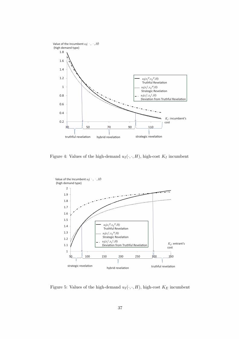
The relationship between the investment cost and the value of the incumbent is then inves-
tigated. Figure 4 depicts the relationship between the values of the high-demand incumbent
and its cost of the investment. As explained in Proposition 6.2, the values decrease non-linearly
with investment cost and increase with profit flow. If the cost is small, Truthful Revelation
occurs, whereas if the cost is large, Manipulative Revelation occurs. If the cost is moderate, the
incumbent uses a complete mixed strategy, in which λ− Hybrid Revelation for some 0 < λ < 1
is an equilibrium.
Finally, the impact of the value of the incumbent on the investment cost of the entrant
is investigated. Note that the value of the incumbent is affected not only by the own cost of
the incumbent, but also by the cost of the rival because the smaller cost of the entrant, which
pushes forward the investment of the entrant, reduces the value of the incumbent. Figure 5
depicts the relationship between the values of the high-demand incumbent and the cost of the
entrant. As shown shown in Proposition 6.2, if the cost of the entrant is large, then the timing
of the investment of the entrant is late. Since the effect of the investment of the entrant on
the value of the incumbent is negligible, the high-demand incumbent invests truthfully. On the
other hand, the incumbent invests strategically for the case in which the cost of the entrant is
small. For a moderate interval of the cost of the entrant, the incumbent uses a mixed strategy.
8 Conclusion
The present paper examines an investment game for an incumbent and an entrant for optimal
entries into a new market in which only the incumbent has the information of whether the
demand, is high or low, and the entrant predicts the demand by observing the investment timing
28

of the incumbent. Whether the incumbent reveals the information truthfully is investigated while
taking into account the signaling effect by using the concept of a perfect Bayesian equilibrium.
A condition in which the incumbent with information of high demand invests strategically in
the equilibrium is characterized. A condition in which the incumbent to use a mixed strategy
in the equilibrium is also demonstrated.
If the duopoly profit for the high-demand incumbent is small, then the incumbent invests
strategically, whereas the incumbent invests truthfully if the duopoly profit is sufficiently large.
The incumbent also invests strategically, if the volatility or the cost of the incumbent is large,
or if the cost of the entrant is small.
Since this is the first study of signaling model for an investment game under real option
approach, extension of the model would be interesting in future research. Preemptive behavior
should be considered by eliminating the assumption in which the incumbent is the leader and the
entrant is the follower. Other stochastic processes could also be considered in order to extend
the model.
Appendix
Proof of Proposition 3.1: This proposition is derived by a standard calculation of the first
hitting time (see for example Dixit and Pindyck (1994), pp. 315?316). Let t be the first hitting
time at which Xs reaches a fixed threshold x, where X0 = x. Dixit and Pindyck (1994, pp.
315–316) reported that
E[e−rt] =(xx
)β(19)
and
E[
∫ T
0Xse
−rsds] =x
r − µ− x
r − µ
(xx
)β(20)
29

where β is given by Eq. (2). Equation (20) implies that
E[
∫ +∞
TXse
−rsds] = E[
∫ +∞
0Xse
−rsds]− E[
∫ +∞
TXse
−rsds] =x
r − µ
(xx
)β(21)
First, we consider vI(xI , θ). If x > xI , then the incumbent immediately enters the market,
i.e., tI = t. Hence, by the Markov property of the geometric Brownian motion, we have
vI(xI , θ) = E[
∫ ∞
tI
e−r(s−t)πθI1Xsds− e−r(tI−t)KI |Xt = x]
= E[
∫ ∞
te−r(s−t)πθ
I1Xsds−KI |Xt = x]
= E[
∫ ∞
0e−rsπθ
I1Xsds|X0 = x]−KI
=πθI1
r − µx−KI .
If x ≤ xI , then tI is the first hitting time of the stochastic process reaches a fixed threshold
xI . Then, according to the Markov property of the geometric Brownian motion,
vI(xI , θ) = E[
∫ ∞
tI
e−r(s−t)πθI1Xsds− e−r(tI−t)KI |Xt = x]
= E[
∫ ∞
tI
e−rsπθI1Xsds− e−rtIKI |X0 = x]
= E[
∫ ∞
tI
e−rsπθI1Xsds|X0 = x]−KIE[−e−rtI |X0 = x].
Equations (19) and (21) imply that vI(xI , θ) =(
πθI1
r−µxI −KI
)(xxI
)β
Similarly, wI(xE , θ) for x < xE is
wI(xE , θ) = E[
∫ ∞
tE
e−r(s−t)(πθI1 − πθ
I2)Xsds|Xt = x]
= E[
∫ ∞
tE
e−rs(πθI1 − πθ
I2)Xsds|X0 = x]
=πθI1 − πθ
I2
r − µxE
(x
xE
)β
.
Proof of Proposition 3.1:
30

This proposition is derived by solving Eqs. (14) and (15) for πHI2. In this proof, the condition
of Case (a) is shown to be obtainable by solving Eq. (14). The conditions of Case (b) and Case
(c) are obtained in a similar manner.
According to Eq. (4), the inequality (14) is expressed by
vI(xHI ,H)− wI(x
HE ,H) ≥ vI(x
LI ,H)− wI(x
LE ,H),
which can be rewritten as
vI(xHI ,H)− vI(x
LI ,H) ≥ wI(x
HE ,H)− wI(x
LE ,H). (22)
Then, Eq. (5) implies
vI(xHI , H)− vI(x
LI ,H) =
(πHI1
r − µxHI −KI
)(x
xHI
)β
−(
πHI1
r − µxLI −KI
)(x
xLI
)β
.
Substituting Eq. (8) into the above expression, we obtain
vI(xHI ,H)− vI(x
LI , H) = β−β(β − 1)β−1xβK1−β
I (r − µ)−β{(πHI1)
β − ϕ(πLI1)
β}, (23)
where ϕ is defined by Eq. (18). Equation (6) also implies that
wI(xHE ,H)− wI(x
LE ,H) =
πHI1 − πH
I2
r − µxHE
(x
xHE
)β
−πHI1 − πH
I2
r − µxLE
(x
xLE
)β
(24)
According to Eq. (1), xHE and xLE are given by
xHE = x∗E(1) =β
β−1r−µπHE2
KE , xLE = x∗E(0) =β
β−1r−µπLE2
KE .
Hence, by substituting these expressions into Eq. (25), we obtain
wI(xHE ,H)−wI(x
LE ,H) = β1−β(β−1)β−1xβK1−β
E (r−µ)−β(πHI1−πH
I2){(πHI1)
β−1−(πLI1)
β−1}. (25)
According to Eqs. (23) and (25), inequality (22) implies that
K1−βI {(πH
I1)β − ϕ(πL
I1)β} ≥ βK1−β
E (πHI1 − πH
I2){(πHI1)
β−1 − (πLI1)
β−1}.
31
Consequently, this yields
πHI2 ≥ πH
I1 −1
β
{(πH
I1)β − ϕ(πL
I1)β
(πHI1)
β−1 − (πLI1)
β−1
}(KE
KI
)β−1
,
which completes the proof.
References
Brennan, M. J., and E. S. Schwartz (1985): “Evaluating Natural Resource Investments,”
The Journal of Business, 58(2), 135–157.
Dixit, A. K., and R. S. Pindyck (1994): Investment under Uncertainty. Princeton University
Press.
Grenadier, S. R. (1996): “The Strategic Exercise of Options: Development Cascades and
Overbuilding in Real Estate Markets,” Journal of Finance, 51(5), 1653–1679.
(1999): “Information Revelation Through Option Exercise,” The Review of Financial
Studies, 12(1), 95–130.
Grenadier, S. R., and A. Malenko (2010): “Real Options Signaling Games with Applica-
tions to Corporate Finance,” Discussion Paper.
Grenadier, S. R., and N. Wang (2005): “Investment Timing, Agency and Information,”
Journal of Financial Economics, 75, 493–533.
Hsu, Y.-W., and B. M. Lambrecht (2007): “Preemptive Patenting under Uncertainty and
Asymmetric Information,” Annals of Operations Research, 151, 5–28.
Huisman, K. J. M. (2001): Technology and Investment: A Game Theoretic Real Options
Approach. Kluwer Academic Publishers.
32

Huisman, K. J. M., and P. M. Kort (1999): “Effect of Strategic Interactions on the Option
Value of Waiting,” Tilburg University.
Kijima, M., and T. Shibata (2002): “Real Options in a Duopoly Market with General Volatil-
ity Structure,” 2002.
Kong, J. J., and Y. K. Kwok (2007): “Real Options in Strategic Investment Games between
two Asymmetric Firms,” European Journal of Operational Research, 181, 967–985.
Kulatilaka, N., and E. C. Perotti (1998): “Strategic Growth Options,” Management
Science, 44(8), 1021–1031.
Lambrecht, B., and W. Perraudin (2003): “Real Options and Preemption under Incomplete
Information,” Journal of Economic Dynamics and Control, 27, 619–643.
McDonald, R. L., and D. R. Siegel (1985): “Investment and the Valuation of Firms When
There Is An Option to Shut Down,” International Economic Review, 26(2), 331–349.
Morellec, E., and N. Schurhoff (2011): “Corporate investment and financing under asym-
metric information,” Journal of Financial Economics, 99(2), 262–288.
Pawlina, G., and P. Kort (2006): “Real Options in an Asymmetric Duopoly: Who Benefits
from Your Competitive Disadvantage?,” Journal of Economics and Management, 15, 1–35.
Shibata, T. (2009): “Investment timing, asymmetric information, and audit structure: a real
options framework,” Journal of Economic Dynamics and Control, 33, 903–921.
Shibata, T., and M. Nishihara (2010): “Dynamic investment and capital structure under
manager-shareholder conflict,” Journal of Economic Dynamics and Control, 34, 158–178.
Smets, F. (1991): “Exporting versus FDI: The effect of uncertainty, irreversibilities and strate-
gic interactions,” Working Paper, Yale University.
33

Smit, H. T. J., and L. Trigeorgis (2002): “Strategic Delay in a Real Options Model of R &
D Competition,” The Review of Economic Studies, 69, 729–747.
34

Figure 1: Values of the high-demand incumbent uI(·, ·,H) and the duopoly profit of the high-
demand incumbent πHI2
35

0
0.1
0.2
0.3
0.4
0.5
0.6
0.7
0.8
0.9
1
0 2 4 6 8 10 12
strategic revela on truthful revela onhybrid revela on
I2H : incumbent’s profit
for duopoly (high demand)
Figure 2: Probability of investment of the high-demand incumbent at the optimal timing for
the high demand and the duopoly profit of the high-demand incumbent πHI2
volatility0.4
0.8
1.2
1.6
2
2.4
2.8
3.2
0 0.05 0.1 0.15 0.2 0.25 0.3 0.35 0.4
strategic revela ontruthful revela on hybrid revela on
Value of the Incumbent uI( · , · , H)(high demand type)
uI(xIH,xE
H,H)
Truthful Revela on
uI(xIL,xE
M,H)
Strategic Revela on
uI(xIL,xE
L,H)
Devia on from Truthful Revela on
Figure 3: Values of the high-demand uI(·, ·,H), high-volatility σincumbent
36
0.2
0.4
0.6
0.8
1
1.2
1.4
1.6
1.8
30 50 70 90 110
strategic revela ontruthful revela on hybrid revela on
Value of the Incumbent uI( · , · , H)(high demand type)
uI(xIH,xE
H,H)
Truthful Revela on
uI(xIL,xE
M,H)
Strategic Revela on
uI(xIL,xE
L,H)
Devia on from Truthful Revela on
KI : incumbent’s
cost
Figure 4: Values of the high-demand uI(·, ·,H), high-cost KI incumbent
1
1.1
1.2
1.3
1.4
1.5
1.6
1.7
1.8
1.9
2
50 100 150 200 250 300 350
strategic revela on truthful revela onhybrid revela on
Value of the Incumbent uI( · , · , H)(high demand type)
uI(xIH,xE
H,H)
Truthful Revela on
uI(xIL,xE
M,H)
Strategic Revela on
uI(xIL,xE
L,H)
Devia on from Truthful Revela onKE: entrant’s
cost
Figure 5: Values of the high-demand uI(·, ·,H), high-cost KE incumbent
37