Real options

Part of material is borrowed from Aswath Damodaran’s website

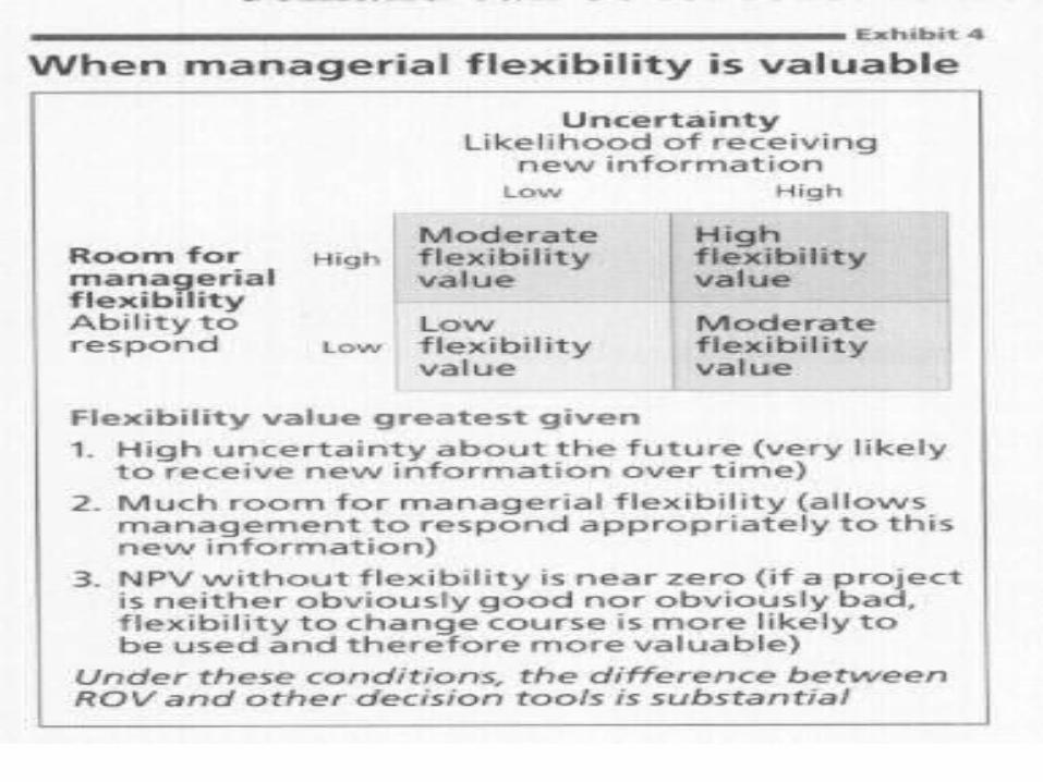
There are three areas in particular where traditional DCF, most widely articulated as the net present value rule (NPV), comes up short versus options theory: Flexibility. Flexibility is the ability to defer, abandon,

expand, or contract an investment. Contingency. This is a situation when future

investments are contingent on the success of today’s investment. Managers may make investments today—even those deemed to be NPV negative—to access future investment opportunities.

Volatility. In options theory, higher volatility —because of asymmetric payoff schemes—leads to higher option value.

Some examples of business situations that can be modeled as real options: Waiting to invest options, as in the case of a tradeoff

between immediate plant expansion (and possible losses from decreased demand) and delayed expansion (and possible lost revenues) 

Growth options, as in the decision to invest in entry into a new market 

Flexibility options, as in the choice between building a single centrally located facility or building two facilities in different locations 

Exit options, as in the decision to develop a new product in an uncertain market 

Learning options, as in a staged investment in advertising.

Advantages of using real options

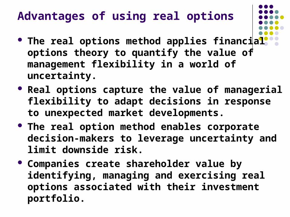
The real options method applies financial options theory to quantify the value of management flexibility in a world of uncertainty.

Real options capture the value of managerial flexibility to adapt decisions in response to unexpected market developments.

The real option method enables corporate decision-makers to leverage uncertainty and limit downside risk.

Companies create shareholder value by identifying, managing and exercising real options associated with their investment portfolio.

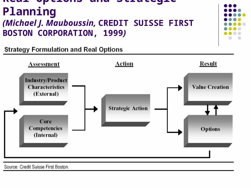
Real Options and Strategic Planning (Michael J. Mauboussin, CREDIT SUISSE FIRST BOSTON CORPORATION, 1999)

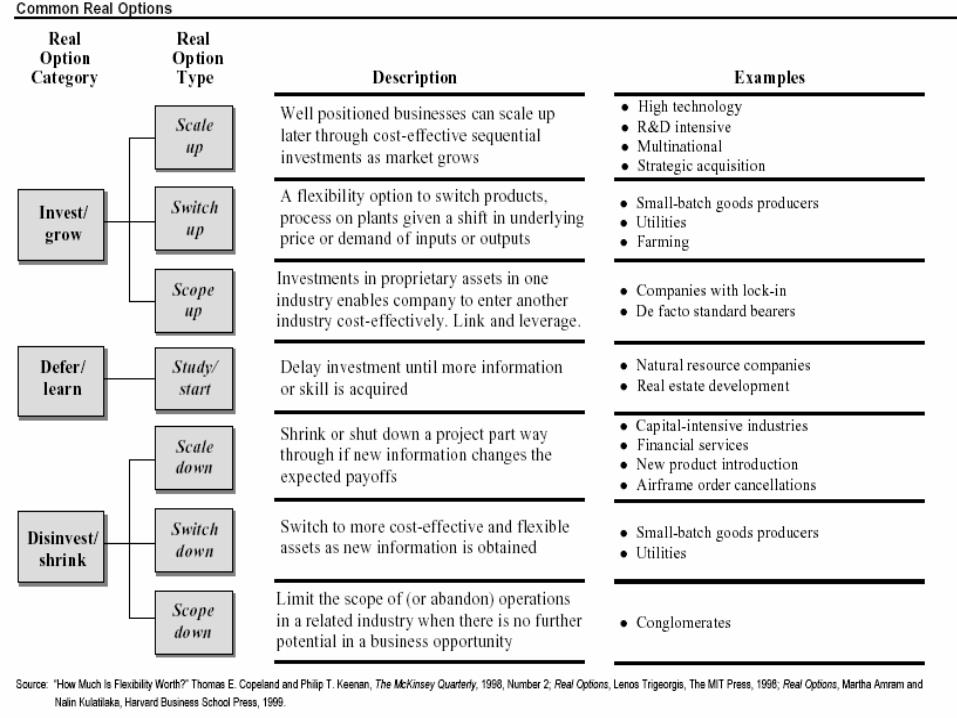
Invest/Grow Options Scale up. The initial investments scale up to future value-

creating opportunities. Scale-up options require prerequisite investments. For example, a distribution company may have valuable scale-up options if the served market grows.

Switch up. A switch( flexibility) option values an opportunity to switch products, process, or plants given a shift in the underlying price or demand of inputs or outputs. A utility company that has the choice between three boilers: natural gas, fuel oil, and dual-fuel. Although the dual-fuel boiler may cost the most, it may be the most valuable, as it allows the company to always use the cheapest fuel.

Scope up. This option values the opportunity to leverage an investment made in one industry into another, related industry. This is also known as link-and-leverage. A company that dominates one sector of e-commerce and leverages that success into a neighboring sector is exercising a scope-up option.

Defer/Learn Options

Study/start. This is a case where management has an opportunity to invest in a particular project, but can wait some period before investing. The ability to wait allows for a reduction in uncertainty, and can hence be valuable. For example, a real estate investor may acquire an option on a parcel of land and exercise it only if the contiguous area is developed.

Disinvest/Shrink Options Scale down. Here, a company can shrink or

downsize a project in midstream as new information changes the payoff scheme. An example would be an airline’s option to abandon a non-profitable route.

Switch down. This option places value on a company’s ability to switch to more cost-effective and flexible assets as it receives new information.

Scope down. A scope-down option is valuable when operations in a related industry can be limited or abandoned based on poor market conditions and some value salvaged. A conglomerate exiting a sector is an example.

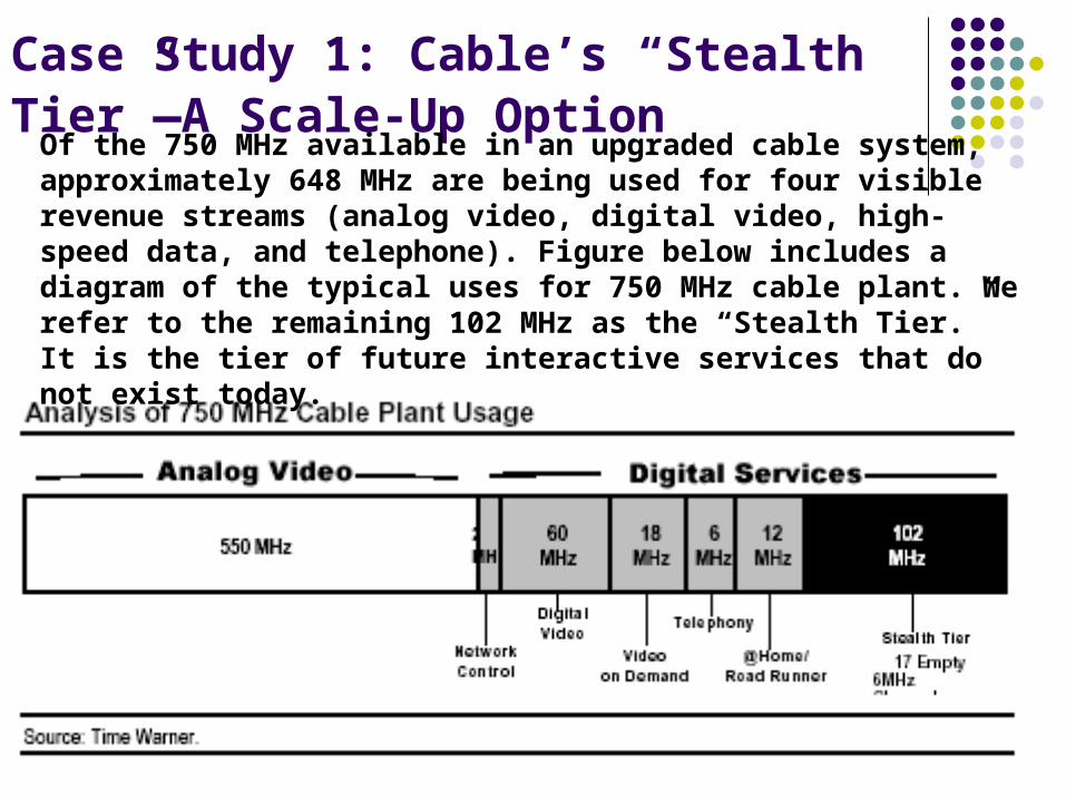
Case Study 1: Cable’s “Stealth Tier”—A Scale-Up Option

Of the 750 MHz available in an upgraded cable system, approximately 648 MHz are being used for four visible revenue streams (analog video, digital video, high-speed data, and telephone). Figure below includes a diagram of the typical uses for 750 MHz cable plant. We refer to the remaining 102 MHz as the “Stealth Tier.” It is the tier of future interactive services that do not exist today.

A Scale-Up Option Lack of visibility does not mean a lack of value. The

Stealth Tier could include services such as video telephone, interactive ecommerce, interactive games, and any other application that requires enormous amounts of bandwidth.

The present value of the four visible revenue streams equals the current public trading value per home passed by cable wire. Accordingly, investors are attributing no value to the 17 empty 6 MHz channels on the interactive tier.

Embedded in the upgrade of the cable plant is a growth option—or scale-up option —that is being overlooked. We know that the additional 102 MHz will be used, we just do not know when or how.

Real options valuation We consider five potential NPV outcomes in our

analysis. To minimize analytical complexity, we hold four

of the five option inputs constant, making the valuation impact of the various NPV assumptions transparent.

We hold volatility (s2) constant at 45% per year (the midpoint of the volatility range), time (t) constant at ten years (cable plant’s life), the risk-free rate (Rf) constant at 5.2%, and the marginal cost (X) per proposed project at 50% of the project’s value.

Real options valuation

Using these variables for each 6 MHz channel in the Stealth Tier, we can determine a range of values. Using just the 17 empty 6 MHz channels available today implies a call option value per home passed of $197-1,979 for the Stealth Tier. The midpoint of this range is $1,088, representing approximately 50% of today’s trading value per home passed.

Case Study 2: Enron—Flexibility Options

In 1998, the electricity prices briefly surged from $40 to an unprecedented $7,000 per megawatt hour in parts of the Midwest. Although the magnitude of this jump was unusual, a combination of capital intensity, transmission constraints, a lack of storage capability, deregulation, and always-uncertain weather has led to a secular increase in electricity price volatility.

Enron learned from the events of 1998. Management realized that its diverse skills and meaningful resources made it uniquely positioned to capitalize on this volatility and immediately began work on a “peaker” plant strategy.

This summer, Enron is slated to open three “peaker” plants—gas-fired electricity generating facilities that have production costs 50-70% higher than the industry’s finest.

The plants, situated at strategic intersections between gas pipelines and the electric grid, are licensed to run only 1,200 hours per year but are much cheaper to build than a normal facility.

In effect, they serve as the equivalent of underground storage in the gas business: they start up when electricity prices reach peak prices.

Real options analysis demonstrated that the flexibility of the peakers is more valuable than their relative inefficiency, given ENE’s wholesale businesses and risk management capabilities.

Case Study 3: Merck and Biogen Contingent Options

In late 1997, Biogen announced that it had signed an agreement with Merck to help it develop and bring to market an asthma drug. Merck paid Biogen $15 million up front, plus the potential of $130 million of milestone payments over several years.

Before the drug becomes commercially viable, Biogen has to shepherd it through the development process. Along the way, Biogen could face expanded tests, a changing asthma drug market, and the risk of abandonment for safety reasons.

Contingent Options

In this case, Merck purchased a stream of options, including scale-up and scale-down (abandonment) options. Drug development represents “options on options,” or a series of contingent options. And Merck’s abandonment option must also be considered. The result is that Merck’s upside is unlimited, while its downside is capped by the payments.

Real options analysis revealed that the deal was worth more than the $145 million of up-front and milestone payments that Merck pledged.

From Biogen’s perspective, the value of the joint venture is the up-front payment plus the expected value of the milestone payments. In effect, Biogen transferred options to Merck that cannot be valued using traditional methods.

Case Study 4: Amazon.comAn Options Smorgasbord

Scope-up options. Amazon has leveraged its position in key markets to launch into similar businesses. For example, it used it market-leading bookselling platform to move into the music business. These can be considered contingency options.

Scale-up options. Flexibility options are part of Amazon’s announced growth in distribution capabilities. The company is adding capacity that will support significantly higher sales volumes in current businesses as well as capacity in potential new ventures. Management believes the cost of this option is attractive when weighed against the potential of disappointing a customer.

Learning options. The company has made a number of acquisitions that may provide the platform for meaningful value creation in the future. The recently acquired business Alexa is an example. Alexa offers Web users a valuable service, suggesting useful alternative Web sites. It also tracks user patterns. Amazon may be able to use this information to better serve its customers in the future.

Equity stakes. Amazon has taken equity stakes in a number of promising businesses, including drugstore.com and pets.com. These new ventures are best valued using options models. Figure below shows a conceptual diagram of how value has been created at Amazon.

The company started by selling books. So there was a DCF value for the book business plus out-of-the-money contingent options on other offerings.

As the book business proved successful, the contingent option on music went from out-of-the-money to in-the-money, spurring the music investment.

As the music business thrived, the company exercised an option to get into videos.

As time has passed, Amazon’s real options portfolio has become more valuable. For example, the recent foray into the auction business, unimaginable one year ago, was contingent on a large base of qualified users.

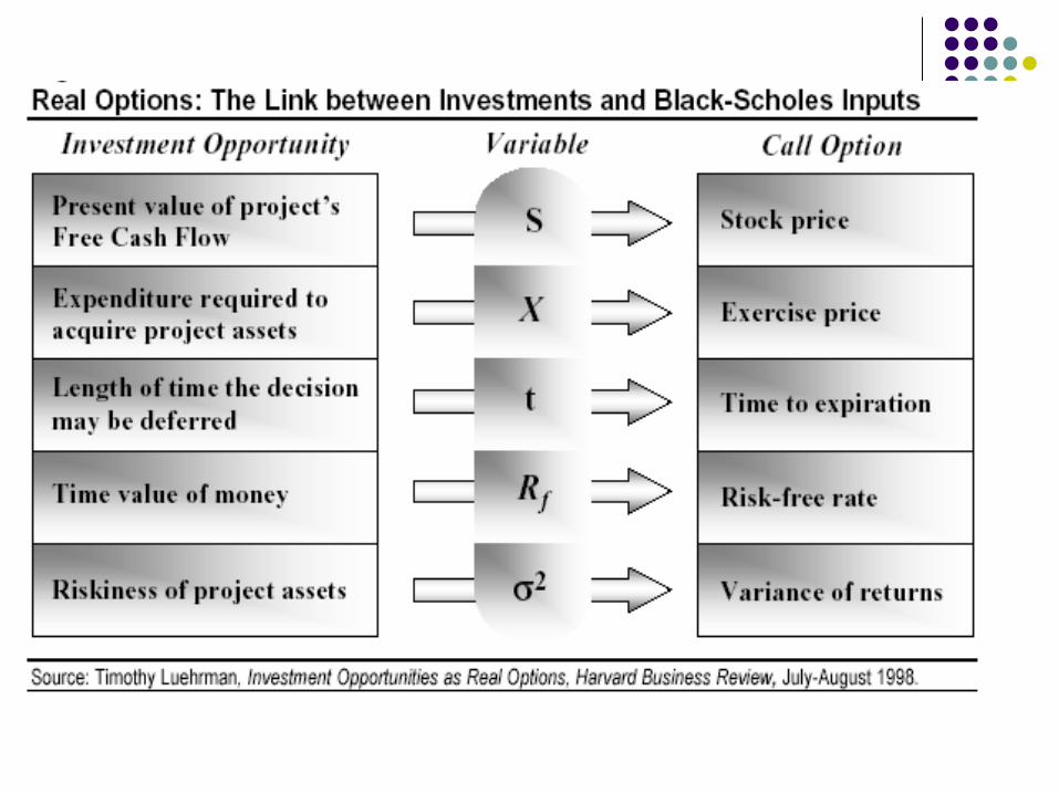
APPLICATIONS OF OPTION PRICING THEORY

TO EQUITY VALUATION

A few caveats on applying option pricing models

1. The underlying asset is not traded. 2. The price of the asset follows a continuous

process. 3. The variance is known and does not

change over the life of the option 4. Exercise is instantaneous

Valuing Equity as an option

Payoff Diagram for Equity as a Call Option. Equity can thus be viewed as a call option the firm, where exercising the option requires that the firm be liquidated and the face value of the debt (which corresponds to the exercise price) paid off.

Application to valuation: A simple example

Assume that a firm whose assets are currently valued at $100 million and that the standard deviation in this asset value is 40%.

Further, assume that the face value of debt is $80 million (It is zero coupon debt with 10 years left to maturity).

If the ten-year treasury bond rate is 10%, how much is the equity worth? What should the

interest rate on debt be?

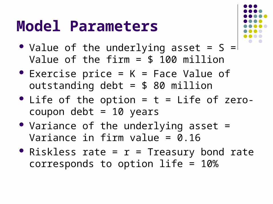
Model Parameters Value of the underlying asset = S = Value of the firm

= $ 100 million Exercise price = K = Face Value of outstanding debt

= $ 80 million Life of the option = t = Life of zero-coupon debt = 10

years Variance of the underlying asset = Variance in firm

value = 0.16 Riskless rate = r = Treasury bond rate corresponds

to option life = 10%

Valuing Equity as a Call Option

)()(C 21 dkNedSN Trf

Tdd

T

Trk

S

df

12

2

1

)5.0()ln(

d1 = 1.5994 N(d1) = 0.9451 d2 = 0.3345 N(d2) = 0.6310 Value of the call = 100 (0.9451) - 80 exp(-0.10)(10)(0.6310) = $75.94MValue of the outstanding debt = $100 - $75.94 = $24.06 millionInterest rate on debt = ($ 80 / $24.06)**1/10 -1 = 12.77%

Valuing equity in a troubled firm:

The parameters of equity as a call option are as follows: Value of the underlying asset = S = Value of the firm =

$ 50 million Exercise price = K = Face Value of outstanding debt =

$ 80 million Life of the option = t = Life of zero-coupon debt = 10

years Variance in the value of the underlying asset = 0.16 Riskless rate = r = Treasury bond rate corresponding to

option life = 10%

d1 = 1.0515 N(d1) = 0.8534 d2 = -0.2135 N(d2) = 0.4155

Value of the call = 50 (0.8534) - 80 exp(-0.10) (10) (0.4155) = $30.44

Value of the bond= $50 - $30.44 = $19.56 million The equity in this firm has substantial value,

because of the option characteristics of equity. This might explain why stock in firms, which are in

Chapter 11 and essentially bankrupt, still has value.

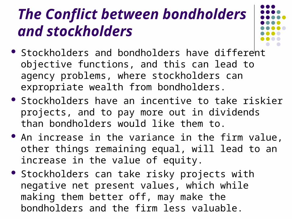
The Conflict between bondholders and stockholders

Stockholders and bondholders have different objective functions, and this can lead to agency problems, where stockholders can expropriate wealth from bondholders.

Stockholders have an incentive to take riskier projects, and to pay more out in dividends than bondholders would like them to.

An increase in the variance in the firm value, other things remaining equal, will lead to an increase in the value of equity.

Stockholders can take risky projects with negative net present values, which while making them better off, may make the bondholders and the firm less valuable.

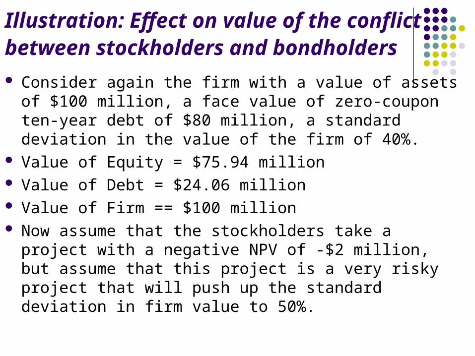
Illustration: Effect on value of the conflict between stockholders and bondholders Consider again the firm with a value of assets of $100

million, a face value of zero-coupon ten-year debt of $80 million, a standard deviation in the value of the firm of 40%.

Value of Equity = $75.94 million Value of Debt = $24.06 million Value of Firm == $100 million Now assume that the stockholders take a project with a

negative NPV of -$2 million, but assume that this project is a very risky project that will push up the standard deviation in firm value to 50%.

Valuing Equity after the Project Value of the firm = S = $ 100 million - $2 million = $ 98 million Exercise price = K = Face Value of debt = $ 80 million Life of the option = t = Life of zero-coupon debt = 10 years Variance in the value of the firm value= 0.25 Riskless rate = r = Treasury bond rate = 10%

Value of Equity = $77.71 Value of Debt = $20.29 Value of Firm = $98.00

The value of equity rises from $75.94 million to $ 77.71 million, even though the firm value declines by $2 million. The increase in equity value comes at the expense of bondholders, who find their wealth decline from $24.06 million to $20.19 million.

Illustration: Effects on equity of a

conglomerate merger

Firm A Firm B

Value of the firm $100 million $ 150 million Face Value of Debt $ 80 million $ 50 million (Zero-coupon debt) Maturity of debt 10 years 10 years Std. Dev. in firm value 40 % 50 % Correlation between firm cash flows 0.4 The ten-year bond rate is 10%.

Variance in combined firm value = (0.4)**2 (0.16) + (0.6)**2 (0.25) + 2 (0.4) (0.6) (0.4) (0.4) (0.5) = 0.154

Valuing the Combined Firm The values of equity and debt in the individual firms and

the combined firm can then be estimated using the option pricing model:

Firm A Firm B Combined Value of equity $75.94 $134.47 $ 207.43 Value of debt $24.06 $ 15.53 $ 42.57 Value of the firm $100.00 $150.00 $ 250.00

The combined value of the equity prior to the merger is $ 210.41 million and it declines to $207.43 million after. The wealth of the bondholders increases by an equal amount. There is a transfer of wealth from stockholders to bondholders, as a consequence of the merger. Thus, conglomerate mergers that are not followed by increases in leverage are likely to see this redistribution of wealth occur across claim holders in the firm

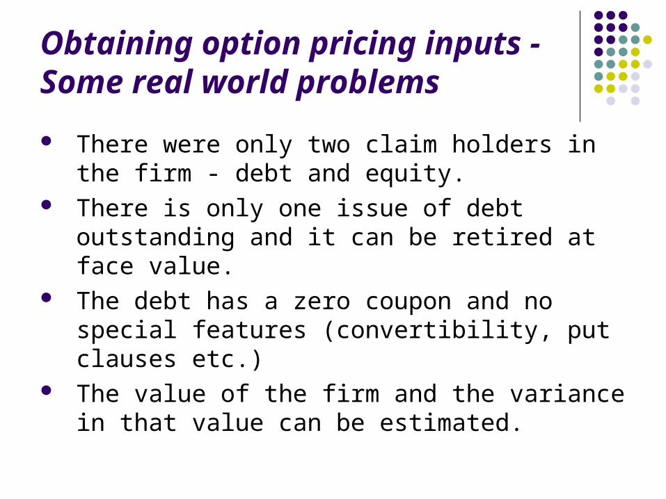
Obtaining option pricing inputs - Some real world problems

There were only two claim holders in the firm - debt and equity.

There is only one issue of debt outstanding and it can be retired at face value.

The debt has a zero coupon and no special features (convertibility, put clauses etc.)

The value of the firm and the variance in that value can be estimated.

Input Estimation Process

Value of the FirmCumulate market values of equity and debt (or) Value the firm using FCFF and WACC (or) Use cumulated market value of assets, if traded.

Variance in Firm Value

If stocks and bonds are traded,

If not traded, use variances of similarly rated bonds. Use average firm value variance from the industry in which company operates.

Maturity of the DebtFace value weighted duration of bonds outstanding (or) If not available, use weighted maturity

2 2 2 22firm e e d d e d e d ed

2 e

e

2d

d

= w + w + 2 w w

Where = variance in the stock price

w = MV weight of Equity

= the variance in the bond price

w = MV weight of debt

Valuing Equity as an option - The

example of an airline The airline owns routes in North America, Europe and South

America, with the following estimates of current market value:

North America $ 400 million Europe $ 500 million South America $ 100 million

It has four debt issues outstanding with the following characteristics:

Maturity Face Value Coupon Duration 20 year debt $ 100 mil 11% 14.1 years 15 year debt $ 100 mil 12% 10.2 years 10 year debt $ 200 mil 12% 7.5 years 1 year debt $ 800 mil 12.5% 1 year

Valuing Equity as an option - The example of an airline

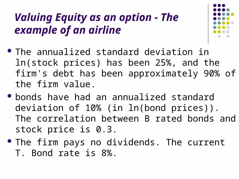
The annualized standard deviation in ln(stock prices) has been 25%, and the firm's debt has been approximately 90% of the firm value.

bonds have had an annualized standard deviation of 10% (in ln(bond prices)). The correlation between B rated bonds and stock price is 0.3.

The firm pays no dividends. The current T. Bond rate is 8%.

Valuing Equity as an option - The example of an airline

Step 1: Value of the firm = 400 + 500 + 100 = 1,000 million Step 2: Average duration = (100/1200) * 14.1 + (100/1200) *

10.2 + (200/1200) * 7.5 + (800/1200) * 1 = 3.9417 years Step 3: Value of debt = 100 + 100 + 200 + 800 = 1,200 million Step 4: Estimate the variance in the value of the firm =

Step 5: Value equity as an option

d1 = 0.7671 N(d1) = 0.7784

d2 = 0.5678 N(d2) = 0.7148

C=1000(0.7784)-1200exp(-0.08)(3.9417)(0.7148)= $ 152.63M

2 2 2 2(.1) (.25) + (.9) (.10) + 2 (.1)(.9)(.3) (.25)(.10) = 0.010075

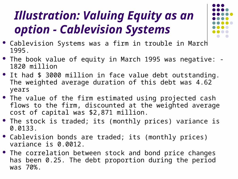
Illustration: Valuing Equity as an option - Cablevision Systems

Cablevision Systems was a firm in trouble in March 1995. The book value of equity in March 1995 was negative: - 1820

million It had $ 3000 million in face value debt outstanding. The

weighted average duration of this debt was 4.62 years The value of the firm estimated using projected cash flows to

the firm, discounted at the weighted average cost of capital was $2,871 million.

The stock is traded; its (monthly prices) variance is 0.0133. Cablevision bonds are traded; its (monthly prices) variance is

0.0012. The correlation between stock and bond price changes has

been 0.25. The debt proportion during the period was 70%.

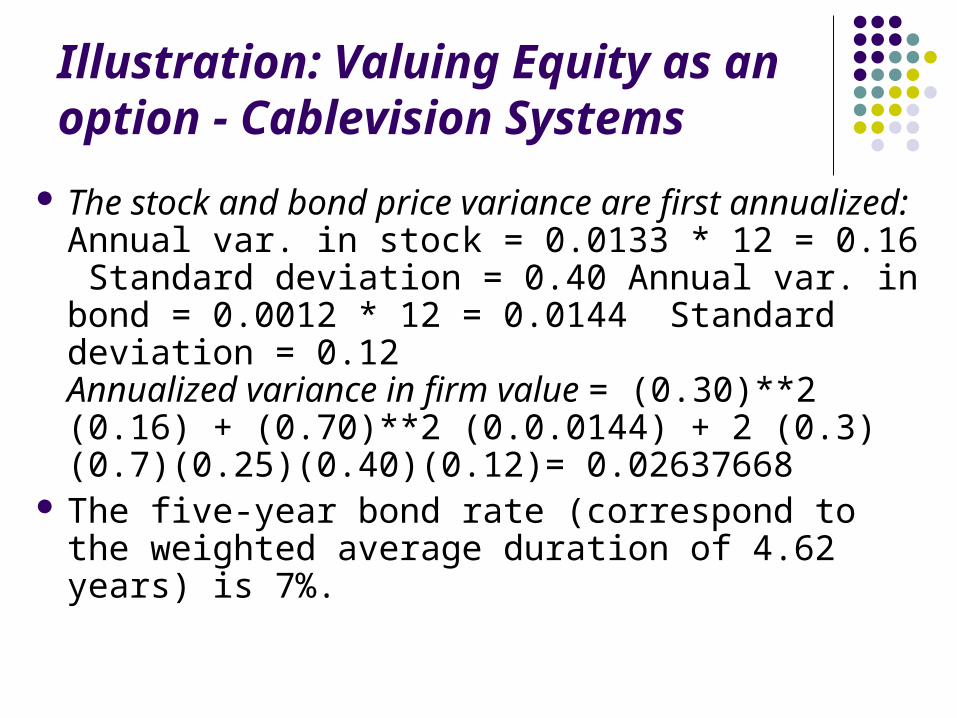
Illustration: Valuing Equity as an option - Cablevision Systems

The stock and bond price variance are first annualized: Annual var. in stock = 0.0133 * 12 = 0.16 Standard deviation = 0.40 Annual var. in bond = 0.0012 * 12 = 0.0144 Standard deviation = 0.12 Annualized variance in firm value = (0.30)**2 (0.16) + (0.70)**2 (0.0.0144) + 2 (0.3) (0.7)(0.25)(0.40)(0.12)= 0.02637668

The five-year bond rate (correspond to the weighted average duration of 4.62 years) is 7%.

Illustration: Valuing Equity as an option - Cablevision Systems

The parameters of equity as a call option are as follows: Value of the firm = S = Value of the firm = $ 2871 million Exercise price = K = Face Value of debt = $ 3000 million Life of the option = t = Weighted average duration of debt = 4.62 years Variance in the value of the underlying asset = 0.0264 Riskless rate = r = Treasury bond rate corresponding to option life = 7%

d1 = 0.9910 N(d1) = 0.8391 d2 = 0.6419 N(d2) = 0.7391

C= 2871(0.8391) - 3000 exp(-0.07)(4.62) (0.7395) = $ 817 million

Cablevision's equity was trading at $1100 million in March 1995.

Valuing Natural Resource

Options/ Firms

Valuing Natural Resource Options/ Firms

In a natural resource investment, the underlying asset is the resource and the value of the asset is based upon two variables - the quantity of the resource that is available in the investment and the price of the resource.

In most such investments, there is a cost associated with developing the resource, and the difference between the value of the asset extracted and the cost of the development is the profit to the owner of the resource.

Defining the cost of development as X, and the estimated value of the resource as V, the potential payoffs on a natural resource option can be written as follows: = V - X if V > X = 0 if V<X

Input Estimation Process

1. Value of Available Reserves of the Resource

Expert estimates; The present value of the after-tax cash flows from the resource are then estimated.

2. Cost of Developing Reserve (Strike Price)

Past costs and the specifics of the investment

3. Time to Expiration Relinquishment Period: if asset has to be relinquished at a point in time.

Time to exhaust inventory - based upon inventory and capacity output.

4. Variance in value of underlying asset

Based upon variability of the price of the resources and variability of available reserves

5. Net Production Revenue (Dividend Yield)

Net production revenue every year as percent of market value.

6. Development Lag Calculate present value of reserve based upon the lag.

Valuing Natural Resource Options/ Firms

*

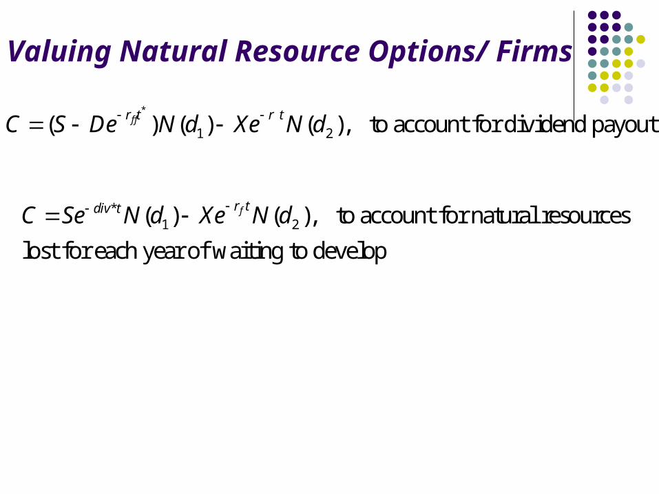
1 2( ) ( ) ( ), to account for dividend payoutf fr t r tC S De N d Xe N d

*1 2( ) ( ), to account for natural resources

lost for each year of waiting to develop

fr tdiv tC Se N d Xe N d

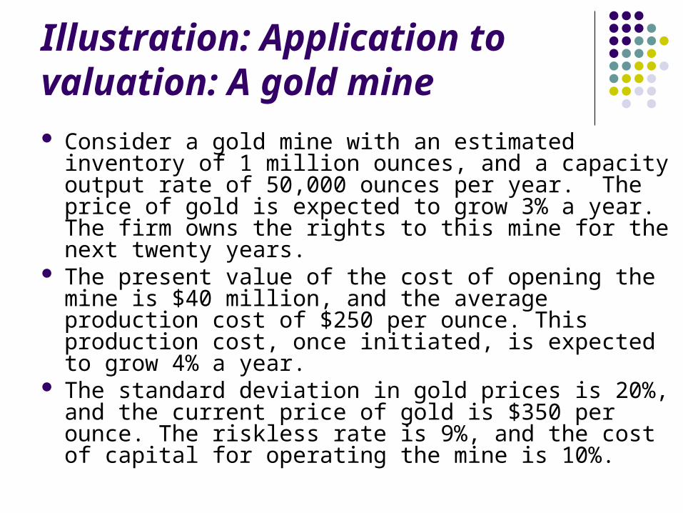
Illustration: Application to valuation: A gold mine Consider a gold mine with an estimated inventory of 1

million ounces, and a capacity output rate of 50,000 ounces per year. The price of gold is expected to grow 3% a year. The firm owns the rights to this mine for the next twenty years.

The present value of the cost of opening the mine is $40 million, and the average production cost of $250 per ounce. This production cost, once initiated, is expected to grow 4% a year.

The standard deviation in gold prices is 20%, and the current price of gold is $350 per ounce. The riskless rate is 9%, and the cost of capital for operating the mine is 10%.

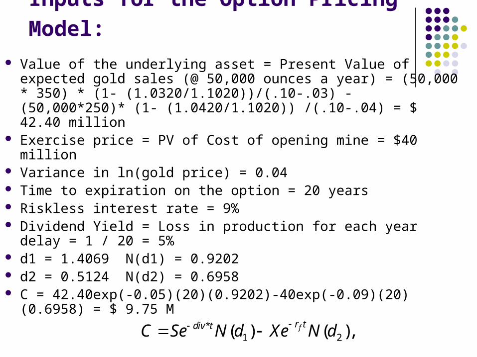
Inputs for the Option Pricing Model: Value of the underlying asset = Present Value of expected gold

sales (@ 50,000 ounces a year) = (50,000 * 350) * (1- (1.0320/1.1020))/(.10-.03) - (50,000*250)* (1- (1.0420/1.1020)) /(.10-.04) = $ 42.40 million

Exercise price = PV of Cost of opening mine = $40 million Variance in ln(gold price) = 0.04 Time to expiration on the option = 20 years Riskless interest rate = 9% Dividend Yield = Loss in production for each year delay = 1 /

20 = 5% d1 = 1.4069 N(d1) = 0.9202 d2 = 0.5124 N(d2) = 0.6958 C = 42.40exp(-0.05)(20)(0.9202)-40exp(-0.09)(20)(0.6958) = $

9.75 M *

1 2( ) ( ), fr tdiv tC Se N d Xe N d

Illustration 10: Valuing an oil reserve

Consider an offshore oil property with an estimated oil reserve of 50 million barrels of oil, where the present value of the development cost is $12 per barrel and the development lag is two years.

The firm has the rights to exploit this reserve for the next twenty years and the marginal value per barrel of oil is $12 per barrel currently (Price per barrel - marginal cost per barrel).

Once developed, the net production revenue each year will be 5% of the value of the reserves. The riskless rate is 8% and the variance in ln(oil prices) is 0.03.

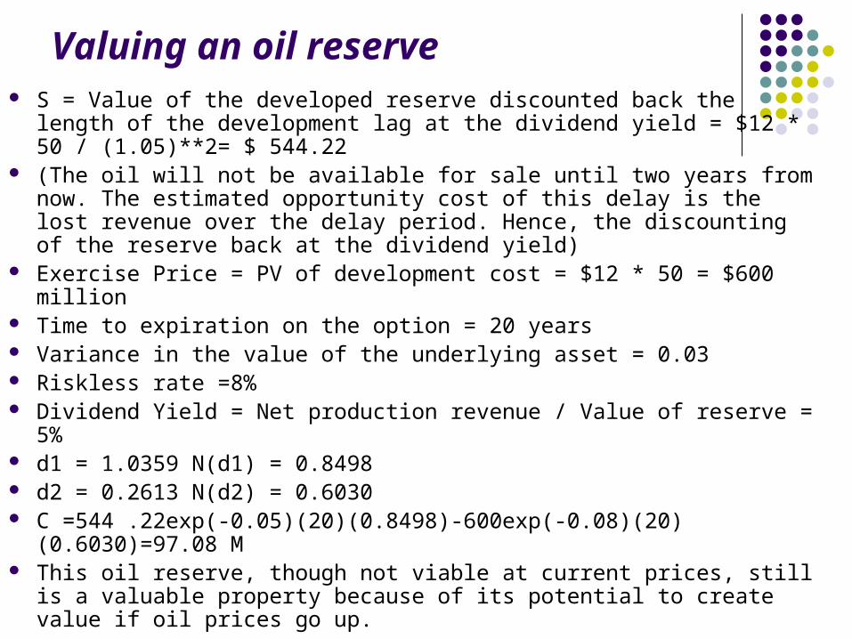
Valuing an oil reserve S = Value of the developed reserve discounted back the length of the

development lag at the dividend yield = $12 * 50 / (1.05)**2= $ 544.22 (The oil will not be available for sale until two years from now. The

estimated opportunity cost of this delay is the lost revenue over the delay period. Hence, the discounting of the reserve back at the dividend yield)

Exercise Price = PV of development cost = $12 * 50 = $600 million Time to expiration on the option = 20 years Variance in the value of the underlying asset = 0.03 Riskless rate =8% Dividend Yield = Net production revenue / Value of reserve = 5% d1 = 1.0359 N(d1) = 0.8498 d2 = 0.2613 N(d2) = 0.6030 C =544 .22exp(-0.05)(20)(0.8498)-600exp(-0.08)(20)(0.6030)=97.08 M This oil reserve, though not viable at current prices, still is a valuable

property because of its potential to create value if oil prices go up.

Valuing product patents as options A product patent provides the firm with the right to

develop the product and market it. It will do so only if the present value of the expected

cash flows from the product sales exceed the cost of development.

If this does not occur, the firm can shelve the patent and not incur any further costs.

If I is the present value of the costs of developing the product, and V is the present value of the expected cash flows from development, the payoffs from owning a product patent can be written as:

Payoff from owning a product patent = V - I if V> I = 0 if V<I

Obtaining the inputs for option valuation

Input Estimation Process

Value of the Underlying Asset

PV of Cash flows from taking project now

Variance in value of underlying asset

Variance in cash flows

Variance in present value from capital budgeting simulation.

Exercise Price on Option Cost of investment on the project.

Expiration of the Option Life of the patent

Dividend Yield Cost of delay, each year of delay translates into one less year of value-creating cashflows

Annual cost of delay = 1/n

Illustration: Valuing a product option

Assume that a firm has the patent rights, for the next twenty years, to a product which requires an initial investment of $ 1.5 billion to develop, and a present value, right now, of cash inflows of only $1 billion.

Assume that a simulation of the project under a variety of technological and competitive scenarios yields a variance in the present value of inflows of 0.03.

The current riskless twenty-year bond rate is 10%.

Valuing the Option Value of the underlying asset = Present value of inflows

(current) = $1,000 million Exercise price = PV of cost of developing product = $1,500 M Time to expiration = Life of the patent = 20 years Variance in underlying asset = Variance in PV of inflows = 0.03 Riskless rate = 10% d1 = 1.1548 N(d1) = 0.8759 d2 = 0.3802 N(d2) = 0.6481 Call Value= 1000 exp(-0.05)(20) (0.8759) -1500 (exp(-0.10)(20)

(0.6481)= $ 190.66 million This suggests that though this product has a negative net present value

currently, it is a valuable product when viewed as an option. This value can then be added to the value of the other assets that the firm possesses, and provides a useful framework for incorporating the value of product options and patents.

Illustration: Valuing a firm with only product options

Consider a bio-technology firm, which has no cash flow-producing assets currently, but has one product in the pipeline that has much promise in providing a treatment for diabetes. The product has not been approved by the FDA, and, even if approved, it could be faced with competition from similar products being worked on by other firms.

The firm, however, would hold the patent rights to this product for the next 25 years. After a series of simulations, the expected present value of the cash inflows is estimated to be $500 million, with a variance of 0.20 (signifying the uncertainty of the process).

The expected present value of the cost of developing the product is estimated to be $400 million. The annual cash flows, once developed, are expected to be 4% of the present value of the inflows. The twenty-five year bond rate is 7%.

Valuing the Option Value of underlying asset = PV of expected cash flows = $ 500

million Exercise price = PV of cost of commercial use = $400 mil Time to expiration on patent rights = 25 years Variance in value of underlying asset = 0.20 Riskless rate = 7% Dividend yield = Expected annual cash flow / PV of cash inflows

= 4% d1 = 1.5532 N(d1) = 0.9398 d2 = -0.6828 N(d2) = 0.2474 C= 500 exp(-0.04)(25)(0.9398)-400exp(-0.07) (25) (0.2474)

=155.66 M The estimated value of this firm is $155.66 million. This is a

more realistic measure of value than traditional discounted cash flow valuation (that would have provided a value of $100 million) because it reflects the underlying uncertainty in the technology and in competition.

Valuing Biogen

The firm is receiving royalties from Biogen discoveries (Hepatitis B and Intron) at pharmaceutical companies. These account for FCFE per share of $1.00 and are expected to grow 10% a year until the patent expires (in 15 years). Using a beta of 1.1 to value these cash flows (leading to a cost of equity of 13.05%), we arrive at a present value per share: Value of Existing Products = $ 12.14

The firm also has a patent on Avonex, a drug to treat multiple sclerosis, for the next 17 years, and it plans to produce and sell the drug by itself. The key inputs on the drug are as follows:

Valuing Biogen PV from Introducing the Drug Now = S = $ 3.422 billion Present Value of Cost of Developing Drug = K = $ 2.875 billion Patent Life = t = 17 years Riskless Rate = r = 6.7% (17-year T.Bond rate) Variance in Expected Present Values = 0.224 (Industry average

firm variance for bio-tech firms) Expected Cost of Delay = y = 1/17 = 5.89% d1 = 1.1362 N(d1) = 0.8720 d2 = -0.8512 N(d2) = 0.2076 Call = 3,422 exp(-0.0589)(17) (0.8720) - 2,875 (exp(-0.067)(17)

(0.2076)= $ 907 million Call from Avonex = $ 907 million/35.5 million = $ 25.55 Biogen Value Per Share = Value of Existing Assets + Value of

Patent = $ 12.14 + $ 25.55 = $37.69

Valuing an Option to Abandon; An Illustration

Assume that a firm is considering taking a 10-year project that requires an initial investment of $ 100 million in a real estate partnership, where the PV of expected cash flows is $110 million. While the NPV of $ 10 million is small, assume that the firm has the option to abandon this project anytime in the next 10 years, by selling its share of the ownership to the other partners for $ 50 million. The variance in the present value of the cash flows from being in the partnership is 0.09.

The value of the abandonment option can be estimated by determining the characteristics of the put option:

Value of the Underlying Asset (S) = $ 110 million Strike Price (K) = Salvage Value from Abandonment = $ 50

million Variance in Underlying Asset’s Value = 0.06 Time to expiration = Period for abandonment option = 10

years Assume that the ten-year riskless rate is 6%, and that the

property is not expected to lose value over the next 10 years. The value of the put option can be estimated as follows:

Call Value = 110 (0.9737) -50 (exp(-0.06)(10) (0.8387) = $ 84.09 million

Put Value= $ 84.09 - 110 + 50 exp(-0.06)(10) = $ 1.53 million The value of this abandonment option has to be added on to

the net present value of the project of $ 10 million, yielding a total net present value with the abandonment option of $11.53 million.

Valuing an Option to Expand: The Home Depot

Assume that The Home Depot is considering opening a small store in France. The store will cost 100 million FF to build, and the present value of the expected cash flows from the store is 80 million FF. Thus, by itself, the store has a NPV of -20 million FF.

By opening this store, the Home Depot acquires the option to expand into a much larger store any time over the next 5 years. The cost of expansion will be 200 million FF, and it will be undertaken only if PV of the expected cash flows exceeds 200 million FF. At the moment, PV of the expected cash flows from the expansion is only 150 million FF. If it were not, the Home Depot would have opened to larger store right away. The Home Depot still does not know much about the market for home improvement products in France, and there is considerable uncertainty about this estimate. The variance is 0.08.

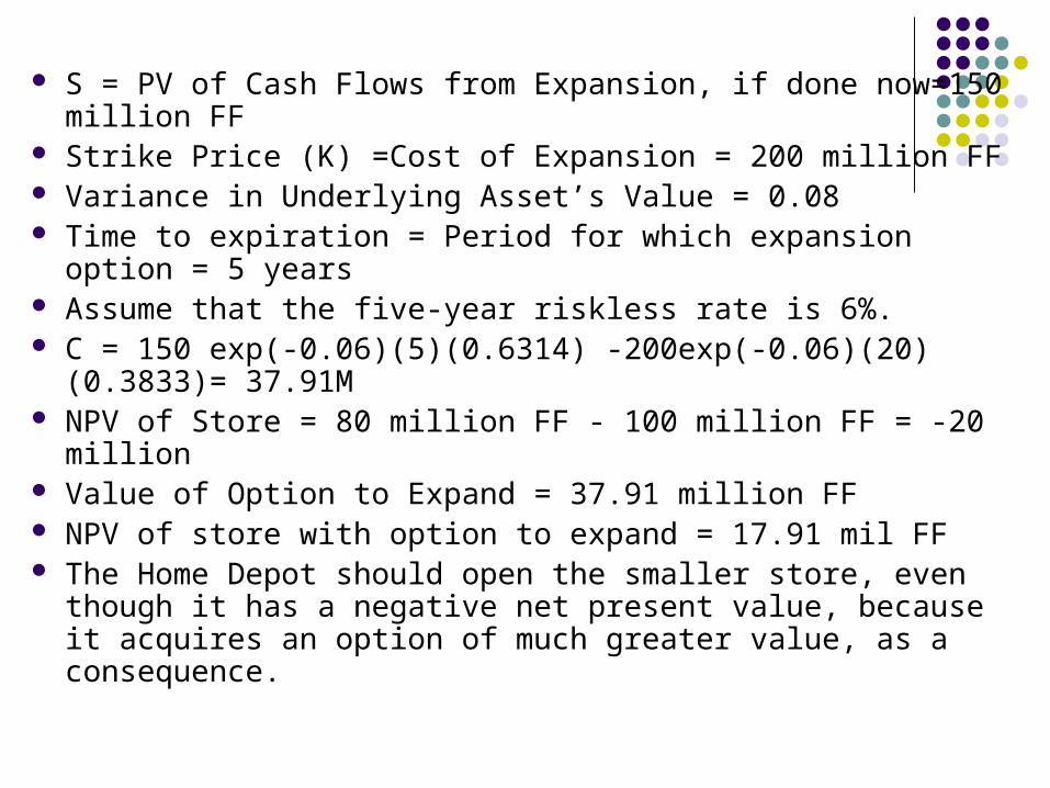
S = PV of Cash Flows from Expansion, if done now=150 million FF

Strike Price (K) =Cost of Expansion = 200 million FF Variance in Underlying Asset’s Value = 0.08 Time to expiration = Period for which expansion option = 5

years Assume that the five-year riskless rate is 6%. C = 150 exp(-0.06)(5)(0.6314) -200exp(-0.06)(20) (0.3833)=

37.91M NPV of Store = 80 million FF - 100 million FF = -20 million Value of Option to Expand = 37.91 million FF NPV of store with option to expand = 17.91 mil FF The Home Depot should open the smaller store, even though

it has a negative net present value, because it acquires an option of much greater value, as a consequence.