real projective iterated function systems - people · michael f. barnsley ·andrew vince ... real...

J Geom AnalDOI 10.1007/s12220-011-9232-x

Real Projective Iterated Function Systems

Michael F. Barnsley · Andrew Vince

Received: 17 March 2010© Mathematica Josephina, Inc. 2011

Abstract This paper contains four main results associated with an attractor of a pro-jective iterated function system (IFS). The first theorem characterizes when a projec-tive IFS has an attractor which avoids a hyperplane. The second theorem establishesthat a projective IFS has at most one attractor. In the third theorem the classical dual-ity between points and hyperplanes in projective space leads to connections betweenattractors that avoid hyperplanes and repellers that avoid points, as well as hyperplaneattractors that avoid points and repellers that avoid hyperplanes. Finally, an index isdefined for attractors which avoid a hyperplane. This index is shown to be a nontrivialprojective invariant.

Keywords Iterated function system · Attractor · Projective space

Mathematics Subject Classification (2000) 28A80

1 Introduction

This paper provides the foundations of a surprisingly rich mathematical theory asso-ciated with the attractor of a real projective iterated function system (IFS). (A realprojective IFS consists of a finite set of projective transformations {fm : P → P }Mm=1

Communicated by Jeffrey Diller.

M.F. Barnsley (�)Department of Mathematics, Australian National University, Canberra, ACT, Australiae-mail: [email protected]: http://www.superfractals.com

M.F. Barnsleye-mail: [email protected]

A. VinceDepartment of Mathematics, University of Florida, Gainesville, FL 32611-8105, USAe-mail: [email protected]

mailto:[email protected]

http://www.superfractals.com



M.F. Barnsley, A. Vince

where P is a real projective space. An attractor is a nonempty compact set A ⊂ Psuch that limk→∞ F k(B) = F (A) = A for all nonempty sets B in an open neighbor-hood of A, where F (B) = ⋃M

m=1 fm(B).) In addition to proving conditions whichguarantee the existence and uniqueness of an attractor for a projective IFS, we alsopresent several related concepts. The first connects an attractor which avoids a hyper-plane with a hyperplane repeller. The second uses information about the hyperplanerepeller to define a new index for an attractor. This index is both invariant under pro-jective transformations and nontrivial, which implies that it joins the cross ratio andHausdorff dimension as nontrivial invariants under the projective group. Thus, theseattractors belong in a natural way to the collection of geometrical objects of classicalprojective geometry.

The definitions that support expressions such as “iterated function system”, “at-tractor”, “basin of attraction” and “avoids a hyperplane”, used in this Introduction,are given in Sect. 3.

Iterated function systems are a standard framework for describing and analyzingself-referential sets such as deterministic fractals [2, 7, 22] and some types of ran-dom fractals [10]. Attractors of affine IFSs have many applications, including imagecompression [3, 8, 21] and geometric modeling [14]. They relate to the theory of thejoint spectral radius [12] and to wavelets [11]. Projective IFSs have more degrees offreedom than comparable affine IFSs [5] while the constituent functions share geo-metrical properties such as preservation of straight lines and cross ratios. ProjectiveIFSs have been used in digital imaging and computer graphics (see, for example, [6]),and they may have applications to image compression, as proposed in [4, p. 10]. Pro-jective IFSs can be designed so that their attractors are smooth objects such as arcsof circles and parabolas, and rough objects such as fractal interpolation functions.

The behavior of attractors of projective IFSs appears to be complicated. In com-puter experiments conducted by the authors, attractors seem to come and go in a mys-terious manner as parameters of the IFS are changed continuously. See Example 4 inSect. 4 for an example that illustrates such phenomena. The intuition developed foraffine IFSs regarding the control of attractors seems to be wrong in the projectivesetting. Our theorems provide insight into such behavior.

One key issue is the relationship between the existence of an attractor and the con-tractive properties of the functions of the IFS. In a previous paper [1] we investigatedthe relationship between the existence of attractors and the existence of contractivemetrics for IFSs consisting of affine maps on R

n. We established that an affine IFS Fhas an attractor if and only if F is contractive on all of R

n. In the present paper wefocus on the setting where X = P

n is real n-dimensional projective space and eachfunction in F is a projective transformation. In this case F is called a projective IFS.

Our first main result, Theorem 1, provides a set of equivalent characterizations of aprojective IFS that possesses an attractor that avoids a hyperplane. The adjoint F t ofa projective IFS F is defined in Sect. 11, and convex body is defined in Definition 5.An IFS F is contractive on S ⊂ X when F (S) ⊂ S and there is a metric on S withrespect to which all the functions of the IFS are contractive; see Definition 3. For aset X in a topological space, X denotes its closure, and int(X) denotes its interior.

Theorem 1 If F is a projective IFS on Pn, then the following statements are equiva-

lent.


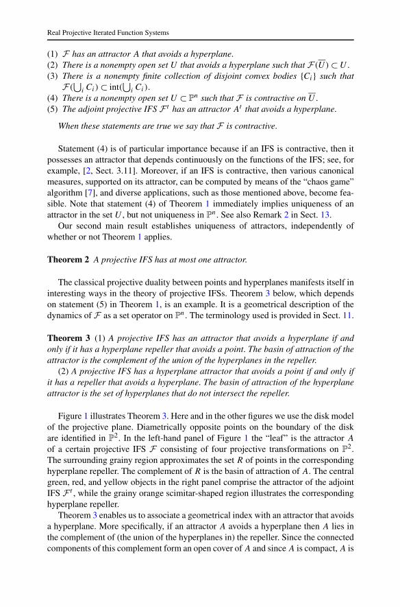
(1) F has an attractor A that avoids a hyperplane.(2) There is a nonempty open set U that avoids a hyperplane such that F (U) ⊂ U .(3) There is a nonempty finite collection of disjoint convex bodies {Ci} such that

F (⋃

i Ci) ⊂ int(⋃

i Ci).(4) There is a nonempty open set U ⊂ P

n such that F is contractive on U .(5) The adjoint projective IFS F t has an attractor At that avoids a hyperplane.

When these statements are true we say that F is contractive.

Statement (4) is of particular importance because if an IFS is contractive, then itpossesses an attractor that depends continuously on the functions of the IFS; see, forexample, [2, Sect. 3.11]. Moreover, if an IFS is contractive, then various canonicalmeasures, supported on its attractor, can be computed by means of the “chaos game”algorithm [7], and diverse applications, such as those mentioned above, become fea-sible. Note that statement (4) of Theorem 1 immediately implies uniqueness of anattractor in the set U , but not uniqueness in P

n. See also Remark 2 in Sect. 13.Our second main result establishes uniqueness of attractors, independently of

whether or not Theorem 1 applies.

Theorem 2 A projective IFS has at most one attractor.

The classical projective duality between points and hyperplanes manifests itself ininteresting ways in the theory of projective IFSs. Theorem 3 below, which dependson statement (5) in Theorem 1, is an example. It is a geometrical description of thedynamics of F as a set operator on P

n. The terminology used is provided in Sect. 11.

Theorem 3 (1) A projective IFS has an attractor that avoids a hyperplane if andonly if it has a hyperplane repeller that avoids a point. The basin of attraction of theattractor is the complement of the union of the hyperplanes in the repeller.

(2) A projective IFS has a hyperplane attractor that avoids a point if and only ifit has a repeller that avoids a hyperplane. The basin of attraction of the hyperplaneattractor is the set of hyperplanes that do not intersect the repeller.

Figure 1 illustrates Theorem 3. Here and in the other figures we use the disk modelof the projective plane. Diametrically opposite points on the boundary of the diskare identified in P

2. In the left-hand panel of Figure 1 the “leaf” is the attractor A

of a certain projective IFS F consisting of four projective transformations on P2.

The surrounding grainy region approximates the set R of points in the correspondinghyperplane repeller. The complement of R is the basin of attraction of A. The centralgreen, red, and yellow objects in the right panel comprise the attractor of the adjointIFS F t , while the grainy orange scimitar-shaped region illustrates the correspondinghyperplane repeller.

Theorem 3 enables us to associate a geometrical index with an attractor that avoidsa hyperplane. More specifically, if an attractor A avoids a hyperplane then A lies inthe complement of (the union of the hyperplanes in) the repeller. Since the connectedcomponents of this complement form an open cover of A and since A is compact, A is


Fig. 1 (Color online) The image on the left shows the attractor and hyperplane repeller of a projectiveIFS. The basin of attraction of the leaf-like attractor is the black convex region together with the leaf. Theimage on the right shows the attractor and repeller of the adjoint system

actually contained in a finite set of components of the complement. These observa-tions lead to the definition of a geometric index of A, index(A), as is made precise inDefinition 13. This index is an integer associated with an attractor A, not any partic-ular IFS that generates A. As shown in Sect. 12, as a consequence of Theorem 4, thisindex is nontrivial, in the sense that it can take positive integer values other than one.Moreover, it is invariant under PGL(n + 1,R), the group of real, dimension n, pro-jective transformations. That is, index(A) = index(g(A)) for all g ∈ PGL(n + 1,R).

See Remark 3 of Sect. 13 concerning attractors and repellers in the case of affineIFSs. See Remark 4 in Sect. 13 concerning the fact that the Hausdorff dimension ofthe attractor is also an invariant under the projective group.

2 Organization

Since the proofs of our results are quite complicated, this section describes the struc-ture of this paper, including an overview of the proof of Theorem 1.

Section 3 contains definitions and notation related to iterated function systems,and background information on projective space, convex sets in projective space, andthe Hilbert metric.

Section 4 provides examples that illustrate the intricacy of projective IFSs and thevalue of our results. These examples also illustrate the role of the avoided hyperplanein statements (1), (2), and (5) of Theorem 1.

The proof of Theorem 1 is achieved by showing that

(1) ⇒ (2) ⇒ (3) ⇒ (4) ⇒ (1) ⇔ (5).

Section 5 contains the proof that (1) ⇒ (2), by means of a topological argument.Statement (2) states that the IFS F is a “topological contraction” in the sense that itsends a nonempty compact set into its interior.


Section 6 contains the proof of Proposition 4, which describes the action of aprojective transformation on the convex hull of a connected set in terms of its actionon the connected set. This is a key result that is used subsequently.

Section 7 contains the proof that (2) ⇒ (3) by means of a geometrical argument,in Lemmas 2 and 3. Statement (3) states that the compact set, in statement (2), thatis sent into its interior can be chosen to be the disjoint union of finitely many convexbodies. What makes the proof somewhat subtle is that, in general, there is no singleconvex body that is mapped into its interior.

Sections 8 and 9 contain the proof that (3) ⇒ (4). Statement (4) states that, withrespect to an appropriate metric, each function in F is a contraction. The requisitemetric is constructed in two stages. On each of the convex bodies in statement (3),the metric is basically the Hilbert metric as discussed in Sect. 3. How to combinethese metrics into a single metric on the union of the convex bodies is what requiresthe two sections.

Section 10 contains both the proof that (4) ⇒ (1) and the proof of Theorem 2.Section 11 contains the proof that (1) ⇔ (5), namely that F has an attractor if and

only if F t has an attractor. The adjoint IFS F t consists of those projective transfor-mations which, when expressed as matrices, are the transposes of the matrices thatrepresent the functions of F . The proof relies on properties of an operation, calledthe complementary dual, that takes subsets of P

n to subsets of Pn.

Section 11 also contains the proof of Theorem 3, which concerns the relationshipbetween attractors and repellers. The proof relies on classical duality between P

n andits dual Pn, as well as the equivalence of statement (4) in Theorem 1. Note that, if Fhas an attractor A then the orbit under F of any compact set in the basin of attractionof A will converge to A in the Hausdorff metric. Theorem 3 tells us that if A avoidsa hyperplane, then there is also a set R of hyperplanes that repel, under the action ofF , hyperplanes “close” to R. The hyperplane repeller R is such that the IFS F −1,consisting of all inverses of functions in F , when applied to the dual space of P

n, hasR as an attractor. The relationship between the hyperplane repeller of an IFS F andthe attractor of the adjoint IFS F t is described in Proposition 10.

Section 12 considers properties of attractors that are invariant under the projectivegroup PGL(n + 1,R). In particular, we define index(A) of an attractor A that avoidsa hyperplane, and establish Theorem 4 which shows that this index is a nontrivialgroup invariant.

Section 13 contains various remarks that add germane information that could in-terrupt the flow on a first reading. In particular, the topic of non-contractive projectiveIFSs that, nevertheless, have attractors is mentioned. Other areas open to future re-search are also mentioned.

3 Iterated Function Systems, Projective Space, Convex Sets, and the HilbertMetric

3.1 Iterated Function Systems and Their Attractors

Definition 1 Let X be a complete metric space. If fm : X → X, m = 1,2, . . . ,M,

are continuous mappings, then F = (X;f1, f2, . . . , fM) is called an iterated functionsystem (IFS).


To define the attractor of an IFS, first define

F (B) =⋃

f ∈Ff (B)

for any B ⊂ X. By slight abuse of terminology we use the same symbol F for theIFS, the set of functions in the IFS, and for the above mapping. For B ⊂ X, let F k(B)

denote the k-fold composition of F , the union of fi1 ◦ fi2 ◦ · · · ◦ fik (B) over all finitewords i1i2 · · · ik of length k. Define F 0(B) = B.

Definition 2 A nonempty compact set A ⊂ X is said to be an attractor of the IFS Fif

(i) F (A) = A and(ii) there is an open set U ⊂ X such that A ⊂ U and limk→∞ F k(B) = A, for all

compact sets B ⊂ U , where the limit is with respect to the Hausdorff metric.

The largest open set U such that (ii) is true is called the basin of attraction [for theattractor A of the IFS F ].

See Remark 6 in Sect. 13 concerning a different definition of attractor.

Definition 3 A function f : X → X is called a contraction with respect to a metric d

if there is 0 ≤ α < 1 such that d(f (x), f (y)) ≤ α d(x, y) for all x, y ∈ Rn.

An IFS F = (X;f1, f2, . . . , fM) is said to be contractive on a set U ⊂ X ifF (U) ⊂ U and there is a metric d : U × U → [0,∞), giving the same topologyas on U , such that, for each f ∈ F the restriction f |U of f to U is a contraction onU with respect to d .

3.2 Projective Space

Let Rn+1 denote (n + 1)-dimensional Euclidean space and let P

n denote real projec-tive space. Specifically, P

n is the quotient of Rn+1\{0} by the equivalence relation

which identifies (x0, . . . , xn) with (λx0, . . . , λxn) for all nonzero λ ∈ R. Let

φ : Rn+1\{0} → P

n

denote the canonical quotient map. The set (x0, . . . , xn) of coordinates of somex ∈ R

n+1 such that φ(x) = p is referred to as homogeneous coordinates of p. Ifp,q ∈ P

n have homogeneous coordinates (p0, . . . , pn) and (q0, . . . , qn), respectively,and

∑ni=0 piqi = 0, then we say that p and q are orthogonal, and write p⊥q . A hy-

perplane in Pn is a set of the form

H = Hp = {q ∈ Pn : p⊥q = 0} ⊂ P

n,

for some p ∈ Pn.

Definition 4 A set X ⊂ Pn is said to avoid a hyperplane if there exists a hyperplane

H ⊂ Pn such that H ∩ X = ∅.


We define the “round” metric dP on Pn as follows. Each point p of P

n is repre-sented by a line in R

n+1 through the origin, or by the two points ap and bp wherethis line intersects the unit sphere centered at the origin. Then, in the obvious nota-tion, dP(p, q) = min{‖ap − aq‖,‖ap − bq‖} where ‖x − y‖ denotes the Euclideandistance between x and y in R

n+1. In terms of homogeneous coordinates, the metricis given by

dP(p, q) =√

2 − 2|〈p,q〉|‖p‖‖q‖ ,

where 〈·, ·〉 is the usual Euclidean inner product. The metric space (Pn, dP) is com-pact.

A projective transformation f is an element of PGL(n + 1,R), the quotient ofGL(n+ 1,R) by the multiples of the identity matrix. A mapping f : P

n → Pn is well

defined by f (φx) = φ(Lf x), where Lf : Rn+1 → R

n+1 is any matrix representingprojective transformation f . In other words, the following diagram commutes:

Rn+1

φ

Lf

Rn+1

φ

Pn

fP

n.

When no confusion arises we may designate an n-dimensional projective trans-formation f by a matrix Lf ∈ GL(n + 1,R) that represents it. An IFS F =(Pn;f1, f2, . . . , fM) is called a projective IFS if each f ∈ F is a projective trans-formation on P

n.

3.3 Convex Subsets of Pn

We now define the notions of convex set, convex body, and convex hull of a set withrespect to a hyperplane. In Proposition 4 we state an invariance property that plays akey role in the proof of Theorem 1.

If H ⊂ Pn is a hyperplane, then there is a unique hyperplane H ∈ R

n+1 such thatφ(H) = H . If p ∈ P

n\H , there is a unique 1-dimensional subspace p ∈ Rn+1 such

that φ(p) = p. Let u be a unit vector orthogonal to H and W = {x : 〈x,u〉 = 1} be thecorresponding affine subspace of R

n+1. Define a mapping θ : Pn\H → W by letting

θ(p) be the intersection of p with W . Now θ is a surjective mapping from Pn\H

onto the n-dimensional affine space W such that projective subspaces of Pn\H go to

affine subspaces of W . In light of the above, it makes sense to consider Pn\H as an

affine space.

Definition 5 A set S ⊂ Pn\H is said to be convex with respect to a hyperplane H

if S is a convex subset of Pn\H , considered as an affine space as described above.

Equivalently, with notation as in the above paragraph, S is convex with respect to H if


θ(S) is a convex subset of W . A closed set that is convex with respect to a hyperplaneand has nonempty interior is called a convex body.

It is important to distinguish this definition of “convex” from projective convex,which is the term often used to describe a set S ⊂ P

n with the property that if l is aline in P

n then S ∩ l is connected. (See [18, 19] for a discussion of related matters.)

Definition 6 Given a hyperplane H ⊂ Pn and two points x, y ∈ P

n\H , the uniqueline xy through x and y is divided into two closed line segments by x and y. Theone that does not intersect H will be called the line segment with respect to H anddenoted xyH .

Note that C is convex with respect to a hyperplane H if and only if xyH ⊂ C forall x, y ∈ C.

Definition 7 Let S ⊂ Pn and let H be a hyperplane such that S ∩H = ∅. The convex

hull of S with respect to H is

convH (S) = conv(S),

where conv(S) is the usual convex hull of S, treated as a subset of the affine spaceP

n\H . Equivalently, with notation as above, if S′ = conv(θ(S)), where conv denotesthe ordinary convex hull in W , then convH (S) = φ(S′).

We can also describe convH (S) as the smallest convex subset of Pn\H that con-

tains S, i.e., the intersection of all convex sets of Pn\H containing S. The key result

concerning convexity and projective transformations is Proposition 4 in Sect. 6.

3.4 The Hilbert Metric

In this section we define the Hilbert metric associated with a convex body.Let p,q ∈ P

n, with p �= q and with homogeneous coordinates p = (p0, . . . , pn)

and q = (q0, . . . , qn). Any point r on the line pq has homogeneous coordinates ri =α1 pi + α2qi, i = 0,1, . . . , n. The pair (α1, α2) is referred to as the homogeneousparameters of r with respect to p and q . Since the homogeneous coordinates of p andq are determined only up to a scalar multiple, the same is true of the homogeneousparameters (α1, α2).

Let a = (α1, α2), b = (β1, β2), c = (γ1, γ2), d = (δ1, δ2) be any four points onsuch a line in terms of homogeneous parameters. Their cross ratio R(a, b, c, d), interms of homogeneous parameters on the projective line, is defined to be

R(a, b, c, d) =∣∣ γ1 α1γ2 α2

∣∣

∣∣ γ1 β1γ2 β2

∣∣–

∣∣ δ1 α1δ2 α2

∣∣

∣∣ δ1 β1δ2 β2

∣∣. (3.1)

The key property of the cross ratio is that it is invariant under any projective transfor-mation and under any change of basis {p,q} for the line. If none of the four points


is the first base point p, then the homogeneous parameters of the points are (α,1),(β,1), (γ,1), (δ,1) and the cross ratio can be expressed as the ratio of (signed) dis-tances:

R(a, b, c, d) = (γ − α)(δ − β)

(γ − β)(δ − α).

Definition 8 Let K ⊂ Pn be a convex body. Let H ⊂ P

n be a hyperplane such thatH ∩ K = ∅. Let x and y be distinct points in int(K). Let a and b be two distinctpoints in the boundary of K such that xyH ⊂ abH , where the order of the pointsalong the line segment abH is a, x, y, b. The Hilbert metric dK on int(K) is definedby

dK(x, y) = logR(a, b, x, y) = log

( |ay| |bx||ax| |by|

)

.

Here |ay| = ‖a′ − y′‖, |bx| = ‖b′ − x′‖, |ax| = ‖a′ − x′‖, |by| = ‖b′ − y′‖ denoteEuclidean distances associated with any set of collinear points a′, x′, y′, b′ ∈ R

n+1

such that φ(a′) = a, φ(x′) = x, φ(y′) = y, and φ(b′) = b.

A basic property of the Hilbert metric is that it is a projective invariant. See [16,p. 105] for a more complete discussion of the properties of this metric. See Remark 4in Sect. 13 concerning the relationship between the metrics dP and dK and its rele-vance to the evaluation and projective invariance of the Hausdorff dimension.

4 Examples

Example 1 (IFSs with one transformation) Let F = (Pn;f ) be a projective IFS witha single transformation. By Theorem 1 such an IFS has an attractor if and only ifany matrix Lf representing f has a dominant eigenvalue. (The map Lf has a realeigenvalue λ0 with corresponding eigenspace of dimension 1, such that λ0 > |λ| forevery other eigenvalue λ.) For such an IFS the attractor is a single point whose ho-mogeneous coordinates are the coordinates of the eigenvector corresponding to λ0.The hyperplane repeller of F is the single hyperplane φ(E), where E is the span ofthe eigenspaces corresponding to all eigenvalues of Lf except λ0. The attractor ofthe adjoint IFS is also a single point, φ(E⊥), where E⊥ is the unique line throughthe origin in R

n+1 perpendicular to the hyperplane E.

Example 2 (Convex hull caveat) In Theorem 1 the implication (2) ⇒ (3) contains asubtle issue. It may seem, at first sight, to be trivial because surely one could chooseC simply to be the convex hull of U? The following example shows that this is nottrue. Let F = (P1;f1, f2) where

f1 =(

4 01 1

)

, f2 =(−4 0

1 1

)

.

In P1 a hyperplane is just a point. Let H0 = (0

1

)and H∞ = ( 1

0

)be two hyperplanes

and consider the four points p = (−91

), q = (−2

1

), r = (2

1

), and s = (9

1

)in P

1. Let


Fig. 2 (Color online) Projective attractor which includes a hyperplane, and a zoom. See Example 3

C1 be the line segment pqH0and let C2 = rsH0 . There are two possible convex

hulls of C1 ∪ C2, one with respect to the hyperplane H0, for example and the otherwith respect to H∞ for example. It is routine to check that F (C1 ∪ C2) ⊂ C1 ∪ C2but F (convH (C1 ∪ C2)) � convH (C1 ∪ C2), where H is either H0 or H∞. Thus thesituation is fundamentally different from the affine case; see [1].

Example 3 (A non-contractive IFS with an attractor) Theorem 1 leaves open thepossible existence of a non-contractive IFS that, nevertheless, has an attractor. Ac-cording to Theorem 1 such an attractor must have nonempty intersection with ev-ery hyperplane. The following example shows that such an IFS does exist. LetF = (P 2;f1, f2) where

f1 =⎛

⎝1 0 00 2 00 0 2

⎞

⎠ and f2 =⎛

⎝1 0 00 2 cos θ −2 sin θ

0 2 sin θ 2 cos θ

⎞

⎠ ,

and θ/π is irrational. In terms of homogeneous coordinates (x, y, z), the attractor ofF is the line x = 0.

Another example is illustrated in Figure 2, where

f1 =⎛

⎝41 −19 19

−19 41 1919 19 41

⎞

⎠ and f2 =⎛

⎝−10 −1 19−10 21 110 10 10

⎞

⎠ .

Neither function f1 nor f2 has an attractor, but the IFS consisting of both of themdoes. The union A of the points in the red and green lines is the attractor. Since anytwo lines in P

2 have nonempty intersection, the attractor A has nonempty intersec-tion with every hyperplane. Consequently, by Theorem 1 there exists no metric withrespect to which both functions are contractive. In the right panel a zoom is shownwhich displays the fractal structure of the set of lines that comprise the attractor. The


color red is used to indicate the image of the attractor under f1, while green indicatesits image under f2.

Example 4 (Attractor discontinuity) This example consists of a family F = {F (t) :t ∈ R} of projective IFSs that depend continuously on a real parameter t . The exampledemonstrates how behavior of a projective family F may be more complicated thanin the affine case. Let F (t) = (P2;f1, f2, f3) where

f1 =⎛

⎝198t + 199 198t + 198 −198t2 − 297t − 99

0 1 0198 198 −198t − 98

⎞

⎠ ,

f2 =⎛

⎝397 396 −594

0 1 0198 198 −296

⎞

⎠ , and f3 =⎛

⎝595 594 −1485

0 1 0198 198 −494

⎞

⎠ .

This family interpolates quadratically between three IFSs, F (0), F (1), and F (2),each of which has an attractor that avoids a hyperplane. But the IFSs F (0.5) andF (1.5) do not have an attractor. This contrasts with the affine case, where similarinterpolations yield IFSs that have an attractor at all intermediate values of the pa-rameter. For example, if hyperbolic affine IFSs F and G each have an attractor, thenso does the average IFS, (t F + (1 − t)G) for all t ∈ [0,1].

5 Proof that (1) ⇒ (2) in Theorem 1

Lemma 1 (i) If the projective IFS F has an attractor A then there is a nonempty openset U such that A ⊂ U , F (U) ⊂ U , and U is contained in the basin of attraction of A.

(ii) (Theorem 1 (1) ⇒ (2)) If the projective IFS F has an attractor A and there isa hyperplane H such that H ∩ A = ∅, then there is a nonempty open set U such thatA ⊂ U, U ∩ H = ∅, F (U) ⊂ U , and U is contained in the basin of attraction of A.

Proof We prove (ii) first. The proof will make use of the function F −1(X) ={x ∈ P

n : f (x) ∈ X for all f ∈ F }. Note that F −1 takes open sets to open sets, X ⊂(F −1 ◦ F )(X) and (F ◦ F −1)(X) ⊂ X for all X.

Since A is an attractor contained in Pn\H , there is an open set V containing A

such that V is compact, V ⊂ Pn\H , and A = limk→∞ F k(V ). Hence there is an

integer m such that F k(V ) ⊂ V for k ≥ m.Define Vk, k = 0,1, . . . ,m, recursively, going backwards from Vm to V0, as fol-

lows. Let Vm = V and for k = m−1, . . . ,2,1,0, let Vk = V ∩ F −1(Vk+1). If O = V0,then O has the following properties:

(1) O is open,(2) A ⊂ O ,(3) F k(O) ⊂ V for all k ≥ 0.

To check property (2) notice that F (A) = A implies A ⊂ (F −1 ◦ F )(A) =F −1(A). Then A ⊂ V = Vm implies that A ⊂ Vm for all m, in particular A ⊂


V0 = O . To check property (3) notice that Vk ⊂ F −1(Vk+1) implies F (Vk) ⊂(F ◦ F −1)(Vk+1) ⊂ Vk+1. It then follows that F k(O) ⊂ Vk ⊂ V for 0 ≤ k ≤ m. AlsoF k(O) ⊂ F k(V ) ⊂ V for all k > m.

Since A = limn→∞ F n(O), there is an integer K such that F K(O) ⊂ O . LetOk, k = 0,1, . . . ,K, be defined recursively, going backwards from OK to O0, asfollows. Let OK = O , and for k = K − 1, . . . ,2,1,0, let Ok be an open set suchthat

(4) F k(O) ⊂ Ok ,(5) Ok ⊂ P

n\H , and(6) F (Ok) ⊂ Ok+1.

To verify that a set Ok with these properties exists, first note that property (4)holds for k = K . To verify the properties for all k = K − 1, . . . ,2,1,0 induc-tively, assume that Ok, k ≥ 1, satisfies property (4). Using property (4) we haveF k−1(O) ⊂ F −1(F k(O)) ⊂ F −1(Ok) and using property (3) we have F k−1(O) ⊂V ⊂ P

n\H . Now choose Ok−1 to be an open set such that F k−1(O) ⊂ Ok−1 andOk−1 ⊂ F −1(Ok) ∩ (Pn\H). The last inclusion implies F (Ok−1) ⊂ Ok .

We claim that

U =K−1⋃

k=0

Ok

satisfies the properties in the statement of part (ii) of the lemma. (*) By property (5)we have U ∩ H = ∅. By properties (2) and (4) we have A = F k(A) ⊂ F k(O) ⊂ Ok

for each k, which implies A ⊂ U . Last,

F (U) =K−1⋃

k=0

F (Ok) ⊂K⋃

k=1

Ok =K−1⋃

k=1

Ok ∪ OK ⊂ U ∪ O ⊂ U ∪ O0 ⊂ U,

the first inclusion coming from property (6) and the second-to-last inclusion comingfrom property (4) applied to k = 0. This completes the proof that there is a nonemptyopen set U such that A ⊂ U . U ∩ H = ∅, and F (U) ⊂ U . Now note that, by con-struction, U is such that F K(U) ⊂ OK = O and that O lies in V which lies in thebasin of attraction of A, which implies that U is contained in the basin of attractionof A. This completes the proof of (ii).

The proof of (i) is the same as the above proof of (ii), except that Pn\H is replaced

by Pn throughout, and the sentence (*) is omitted. �

6 Projective Transformations of Convex Sets

This section describes the action of a projective transformation on a convex set. Wedevelop the key result, Proposition 4, that is used subsequently.

Proposition 1 states that the property of being a convex subset (with respect to ahyperplane) of a projective space is preserved under a projective transformation.


Proposition 1 Let f : Pn → P

n be a projective transformation. For any two hyper-planes H,H ′ with S ∩H = ∅ and f (S)∩H ′ = ∅, the set S ⊂ P

n is a convex set withrespect to H if and only if f (S) is convex with respect to H ′.

Proof Assume that S is convex with respect to H . To show that f (S) is convex withrespect to H ′ it is sufficient to show, given any two points x′, y′ ∈ f (S), that x′y′

H ′ ⊆f (S). If x = f −1(x′) and y = f −1(y′), then by the convexity of S and the fact thatS ∩ H = ∅, we know that xyH ⊆ S. Hence f (xyH ) ⊆ f (S). Since f (S) ∩ H ′ = ∅,and f takes lines to lines, x′y′

H ′ = f (xyH ) ⊆ f (S).The converse follows since f −1 is a projective transformation. �

Proposition 2 states that convH (S) behaves well under projective transformation.

Proposition 2 Let S ⊂ Pn and let H be a hyperplane such that S ∩ H = ∅. If f :

Pn → P

n is a projective transformation, then

convf (H) f (S) = f (convH (S)).

Proof Since S ⊆ convH (S), we know that f (S) ⊆ f (convH (S)). Moreover, byProposition 1, we know that f (convH (S)) is convex with respect to f (H). Toshow that convf (H) f (S) = f (convH (S)) it is sufficient to show that f (convH (S))

is the smallest convex subset containing f (S), i.e., there is no set C such that C

is convex with respect to f (H) and f (S) ⊆ C � f (convH (S)). However, if sucha set exists, then by applying the inverse f −1 to the above inclusion, we haveS ⊆ f −1(C) � convH (S). Since f −1(C) is convex by Proposition 1, we arrive ata contradiction to the fact that convH (S) is the smallest convex set containing S. �

In general, convH (S) depends on the avoided hyperplane H . But, as Proposition 3shows, it is independent of the avoided hyperplane when S is connected.

Proposition 3 If S ⊂ Pn is a connected set such that S ∩ H = S ∩ H ′ = ∅ for hyper-

planes H,H ′ of Pn, then

convH (S) = convH ′(S).

Proof The fact that S is connected and S ∩ H ′ = ∅ implies that convH (S) ∩ H ′ = ∅.

Therefore convH (S) is the ordinary convex hull of S in (Pn\H)\H ′, which is anaffine n-dimensional space with a hyperplane deleted. Likewise convH ′(S) is theordinary convex hull of S in (Pn\H ′)\H = (Pn\H)\H ′. Therefore, convH (S) =convH ′(S). �

The key result that will be needed, for example, in Sect. 7, is the following.

Proposition 4 Let S ⊂ Pn be a connected set and let H be a hyperplane. If S∩H = ∅

and f : Pn → P

n is a projective transformation such that f (S) ∩ H = ∅, then

convH f (S) = f (convH (S)).

Proof This follows at once from Propositions 2 and 3. �


7 Proof that (2)⇒(3) in Theorem 1

The implication (2)⇒(3) in Theorem 1 is proved in two steps. We show that(2)⇒(2.5)⇒(3) where (2.5) is the following statement.

(2.5) There is a hyperplane H and a nonempty finite collection of nonempty dis-joint connected open sets {Oi} such that F (

⋃i Oi) ⊂ ∪iOi and

⋃i Oi ∩ H = ∅.

Lemma 2 ((2)⇒(2.5)) If there is a nonempty open set U and a hyperplane H

with U ∩ H = ∅ such that F (U) ⊂ U , then there is a nonempty finite collectionof nonempty disjoint connected open sets {Oi} such that F (

⋃i Oi) ⊂ ∪iOi and⋃

i Oi ∩ H = ∅.

Proof Let U = ⋃α Uα , where the Uα are the connected components of U . Let A =

⋂k F k(U) and let {Oi} be the set of Uα that have nonempty intersection with A.

This set is finite because the sets in {Oi} are pairwise disjoint and A is compact.Since F (A) ⊂ A and F (U) ⊂ U , we find that F (

⋃Oi) ⊂ ⋃

i Oi . Since⋃

i Oi ⊂ U

and U ∩ H = ∅, we have⋃

i Oi ∩ H = ∅. �

Lemma 3 ((2.5)⇒(3)): If there is a nonempty finite collection of nonempty disjointconnected open sets {Oi} and a hyperplane H such that F (

⋃i Oi) ⊂ ⋃

i Oi and⋃i Oi ∩ H = ∅, then there is a nonempty finite collection of disjoint convex bodies

{Ci} such that F (⋃

i Ci) ⊂ int(⋃

i Ci).

Proof Assume that there is a nonempty finite collection of nonempty disjoint con-nected open sets {Oi} such that F (

⋃i Oi) ⊂ ⋃

i Oi and⋃

i Oi avoids a hyperplane.Let O = ⋃

i Oi . Since F (O) ⊂ O , it must be the case that, for each f ∈ F and each i,there is an index that we denote by f (i), such that f (Oi) ⊂ Of (i). Since Oi is con-nected and both Oi and f (Oi) avoid the hyperplane H it follows from Proposition 4that

f (convH (Oi)) = convH (f (Oi)) ⊂ convH (Of (i)) ⊂ int(convH (Of (i))).

For each i, let Ci = convH (Oi), so that each Ci is a convex body. Then we have

f (Ci) ⊂ int(Cf (i)).

However, it may occur, for some i �= j , that Ci ∩ Cj �= ∅. In this case Ci ∪ Cj is aconnected set that avoids the hyperplane H , and is such that f (Ci ∪ Cj) also avoidsH. It follows again by Proposition 4 that

convH (f (Ci ∪ Cj )) = f (convH (Ci ∪ Cj )) ⊂ int(conv(Cf (i) ∪ Cf (j)).

Define Ci and Cj to be related if Ci ∩ Cj �= ∅, and let ∼ denote the transitiveclosure of this relation. (That is, if Ci is related to Cj and Cj is related to Ck , thenCi is related to Ck .) From the set {Ci} define a new set U ′ whose elements are

U ′ ={

conv

( ⋃

C∈Z

C

)

: Z is an equivalence class with respect to ∼}

.


By abuse of language, let {Ci} be the set of convex sets in U ′. It may again occur,for some i �= j , that Ci ∩ Cj �= ∅. In this case we repeat the equivalence process. Ina finite number of such steps we arrive at a finite set of disjoint convex bodies {Ci}such that F (∪Ci) ⊂ int(∪Ci). �

Lemmas 2 and 3 taken together imply that (2) ⇒ (3) in Theorem 1.

8 Part 1 of the Proof that (3) ⇒ (4) in Theorem 1

The standing assumption in this section is that statement (3) of Theorem 1 is true.We begin to develop a metric with respect to which F is contractive. The final metricis defined in the next section.

Let U := {C1,C2, . . . ,Cq} be the set of nonempty convex connected componentsin statement (3) of Theorem 1. Define a directed graph (digraph) G as follows. Thenodes of G are the elements of U . For each f ∈ F , there is an edge colored f

directed from node U to node V if f (U) ⊂ int(V ). Note that, for each node U in G,there is exactly one edge of each color emanating from U . Note also that G may havemultiple edges from one node to another and may have loops. (A loop is an edge froma node to itself.)

A directed path in a digraph is a sequence of nodes U0,U1, . . . ,Uk such that thereis an edge directed from Ui−1 to Ui for i = 1,2, . . . , k. Note that a directed path isallowed to have repeated nodes and edges. Let p = U0,U1, . . . ,Uk be a directed path.If f1, f2, . . . , fk are the colors of the successive edges, then we will say that p hastype f1 f2 · · ·fk .

Lemma 4 The graph G cannot have two directed cycles of the same type starting atdifferent nodes.

Proof By way of contradiction assume that U �= U ′ are the starting nodes of twopaths p and p′ of the same type f1 f2 · · ·fk . Recall that the colors are functions ofthe IFS F . If g = fk ◦ fk−1 ◦ · · · ◦ f1 ◦ f0, then the composition g takes the convexset U into int(U) and the convex set U ′ into int(U ′). By the Krein–Rutman theorem[23] this is impossible. More specifically, the Krein–Rutman theorem tells us that ifK is a closed convex cone in R

n+1 and L : Rn+1 → R

n+1 is a linear transformationsuch that L(K) ⊂ int(K), then the spectral radius r(L) > 0 is a simple eigenvalue ofL with an eigenvector v ∈ int(K). �

Each function f ∈ F acts on the set of nodes of G in this way: f (U) = V where(U,V ) is the unique edge of color f starting at U .

Lemma 5 There exists a metric dG on the set of nodes of G such that

(1) dG(U,V ) ≥ 2 for all U �= V and(2) each f ∈ F is a contraction with respect to dG.


Proof Starting from the graph G, construct a directed graph G2 whose set of nodesconsists of all unordered pairs {U,V } of distinct nodes of G. In G2 there is an edgefrom {U,V } to {f (U),f (V )} for all nodes {U,V } in G2 and for each f ∈ F . SinceG has no two directed cycles of the same type starting at different nodes, we knowby Lemma 4 that G2 has no directed cycle. Because of this, a partial order ≺ can bedefined on the node set of G2 by declaring that {U ′,V ′} ≺ {U,V } if there is an edgefrom {U,V } to {U ′,V ′} and then taking the transitive closure. Every finite partiallyordered set has a linear extension (see [15], for example), i.e., there is an ordering <

of the nodes of G2:

{U1,V1} < {U2,V2} < · · · < {Um,Vm}such that if {U,V } ≺ {U ′,V ′} then {U,V } < {U ′,V ′}. Using N(G) to denote the setof nodes of G, define a map dG : N(G) × N(G) → [0,∞) in any way satisfying

(1) dG(U,U) = 0 for all U ∈ N(G),

(2) dG(U,V ) = dG(V,U) for all U,V ∈ N(G), and(3) 2 ≤ dG(U1,V1) < dG(U2,V2) < · · · < dG(Um,Vm) ≤ 4.

Properties (1), (2), and (3) guarantee that dG is a metric on N(G). The fact that2 ≤ dG(Ui,Vi) ≤ 4 for all i guarantees the triangle inequality. If

s = min1≤i<m

dG(Ui,Vi)

dG(Ui+1,Vi+1),

then 0 < s < 1 and, for any f ∈ F , we have

dG(f (U),f (V )) ≤ s dG(U,V )

because {f (U),f (V )} ≺ {U,V } by the definition of the partial order and {f (U),

f (V )} < {U,V } by the definition of linear extension. Hence f is a contraction withrespect to dG for any f ∈ F . �

9 Part 2 of the Proof that (3)⇒(4) in Theorem 1

In this section we construct a metric di on each component Ci of the collection {Ci} ={Ci : i = 1,2, . . . , q} in statement (3) of Theorem 1. We will then combine the metricsdi with the graph metric dG in Sect. 8 to build a metric on

⋃i Ci such that statement

(4) in Theorem 1 is true. Proofs that a projective transformation is contractive withrespect to the Hilbert metric go back to G. Birkhoff [13]; also see P.J. Bushell [17].The next lemma is used to compute the contraction factor for projective maps underthe Hilbert metric.

Lemma 6 If r ≥ α ≥ 0, t ≥ α, and h,h′, s, s′ ∈ (0,1), where s′ = 1 − s, h′ = 1 − h,

and s ≤ h, then log((r+h)(t+s′)(r+s)(t+h′) ) ≤ log(

(α+h)(α+s′)(α+s)(α+h′) ) ≤ 1

α+1 log(hs′sh′ ).

Proof Since we are assuming that s ≤ h, s(1 − h) > 0, and α ≥ 0, it is an easyexercise to show that (α+h)(α+s′)

(α+s)(α+h′) ≥ 1. A bit of algebra can be used to show that N :=


(α+h)(α+s′)(α+s)(α+h′) = (1− h′

α+1 )(1− sα+1 )

(1− s′α+1 )(1− h

α+1 ). If we let α = 0 in the above expression, we observe

that D := hs′sh′ = (1−h′)(1−s)

(1−s′)(1−h).

Since ln(1 − x) = loge(1 − x) = −∑∞j=1

xj

j, whenever |x| < 1, for a logarithm

of any base we see that

log(N)

log(D)= log(1 − h′

α+1 ) + log(1 − sα+1 ) − log(1 − s′

α+1 ) − log(1 − hα+1 )

log(1 − h′) + log(1 − s) − log(1 − s′) − log(1 − h)

=−∑∞

j=1

[h′j

j (α+1)j+ sj

j (α+1)j− s′j

j (α+1)j− hj

j (α+1)j

]

−∑∞j=1

[h′jj

+ sj

j− s′j

j− hj

j

]

= 1

α + 1

∑∞j=1

1(α+1)j−1

[s′jj

+ hj

j− h′j

j− sj

j

]

∑∞j=1

[s′jj

+ hj

j− h′j

j− sj

j

] ≤ 1

α + 1.

Note that the above inequality holds because the assumption s ≤ h implies s′ = 1 −s ≥ 1 − h = h′ and (1 − s)j + hj ≥ (1 − h)j + sj , for all positive integers j. Thus,the series in the numerator and denominator can be compared term by term. Finally,it is a straightforward argument to show the numerator N(α) has the property thatif r ≥ α ≥ 0 and t ≥ α ≥ 0, then (r+h)(t+s′)

(r+s)(t+h′) ≤ (α+h)(α+s′)(α+s)(α+h′) . Thus, log(

(r+h)(t+s′)(r+s)(t+h′) ) ≤

log((α+h)(α+s′)(α+s)(α+h′) ). �

Proposition 5 Let F be a projective IFS and let there be a nonempty finite collectionof disjoint convex bodies {Ci : i = 1,2, . . . , q} such that F (

⋃i Ci) ⊂ int(

⋃i Ci) as in

statement (3) of Theorem 1. For i ∈ {1,2, . . . , q} and f ∈ F , let f (i) ∈ {1,2, . . . , q}be defined by f (Ci) ⊂ Cf (i). Then there is a metric di on Ci , giving the same topol-ogy on Ci as dP, such that

1. (Ci, di) is a complete metric space, for all i = 1,2, . . . , q;2. there is a real 0 ≤ α < 1 such that

df (i)(f (x), f (y)) ≤ αdi(x, y)

for all x, y ∈ Ci , for all i = 1,2, . . . , q, for all f ∈ F ; and3. di(x, y) ≤ 1 for all x, y ∈ Ci and all i = 1,2, . . . , q .

Proof For each Ci there exists a hyperplane Hi such that Hi ∩ Ci = ∅. Let Ci ={x ∈ P

n : dP(x, y) ≤ ε, y ∈ Ci} where ε is chosen so small that (i) Hi ∩ Ci = ∅; and(ii) f (Ci) ⊂ int(Cf (i)) ∀f ∈ F ,∀i ∈ {1,2, . . . , q}.

Given arbitrary x, y ∈ int(Ci), let a, b be the points where the line xy intersects∂Ci and let af , bf be the points where the line f (x)f (y) intersects ∂Cf (i). Let di

denote the Hilbert metric on the interior of Ci for each i, and define

βf,i = min{|xy| : x ∈ ∂Cf (i), y ∈ f (Ci)} > 0, for f ∈ F ,i ∈ {1,2, . . . , q}.


We claim that

df (i)(f (x), f (y)) = ln

( |af f (y)| |f (x)bf ||af f (x)| |f (y)bf |

)

≤ 1

βf,i + 1ln

( |f (a)f (y)| |f (x)f (b)||f (a)f (x)| |f (y)f (b)|

)

= 1

βf,i + 1ln

( |a y| |x b||a x| |y b|

)

= 1

βf,i + 1di (x, y), (9.1)

for all x, y ∈ int(Ci), for all f ∈ F , and all i = 1,2, . . . . Here | · | denotes Euclideandistance as discussed in Sect. 3. The second-to-last equality is the invariance of thecross ratio under a projective transformation. Concerning the inequality, without lossof generality, let |f (a)f (b)| = 1, h := |f (a)f (y)|, and s := |f (a)f (x)|. Moreover,let r := |af f (x)| and t := |f (y)bf |. Finally, let s′ = 1 − s and h′ = 1 −h. Note thats ≤ h < 1. The inequality is now the inequality of Lemma 6.

Now let α = max{ 11+βf,i

: f ∈ F , ∀i = 1,2, . . . , q} < 1. It follows that

df (i)(f (x), f (y)) ≤ αdi(x, y)

for all x, y ∈ Ci , for all i = 1,2, . . . , q, for all f ∈ F . Since Ci ⊂ int(Ci) it followsthat statement (2) in Proposition 5 is true.

Statement (1) follows at once from the fact that the topology generated by theHilbert metric di on Ci as defined above is bi-Lipschitz equivalent to dP; see Re-mark 4.

Since di : Ci ×Ci → R is continuous and Ci ×Ci is compact, it follows that thereis a constant Ji such that di (x, y) ≤ Ji for all x, y ∈ Ci . Let J = maxi Ji , and definea new metric di by di(x, y) = di (x, y)/J for all x, y ∈ Ci . We have that di satisfies(1), (2), and (3) in the statement of Proposition 5. �

Lemma 7 (Theorem 1 (3)⇒(4)) If there is a nonempty finite collection of disjointconvex bodies {Ci} such that F (

⋃i Ci) ⊂ int(

⋃i Ci), as in statement (3) of Theo-

rem 1, then there is a nonempty open set U ⊂ Pn and a metric d : U → [0,∞),

generating the same topology as dP on U , such that F is contractive on U .

Proof Let U = ⋃i int(Ci). Define d : U × U by

d(x, y) ={

di(x, y) if (x, y) ∈ Ci × Ci for some i,

dG(Ci,Cj ) if (x, y) ∈ Ci × Cj for some i �= j,

where the metrics di and dG are defined in Lemma 5 and Proposition 5.First we show that d is a metric on U . We only need to check the triangle inequal-

ity. If x, y and z lie in the same connected component of Ci , the triangle inequalityfollows from Proposition 5. If x, y, and z lie in three distinct components, the triangleinequality follows from Lemma 5. If x, y ∈ Ci and z ∈ Cj for some i �= j , then

d(x, y) + d(y, z) = di(x, y) + dG(Ci,Cj ) ≥ dG(Ci,Cj ) = d(x, z),


d(x, z) + d(z, y) = dG(Ci,Cj ) + dG(Cj ,Ci) ≥ 2 ≥ di(x, y) = d(x, y).

Second we show that F is contractive with respect to d . By Proposition 5 there is0 ≤ α < 1 such that, if x and y lie in the same connected component of U and f ∈ F ,then

d(f (x), f (y)) ≤ α d(x, y).

If x and y lie in different connected components of U , then there are two cases. Iff (x) and f (y) lie in different connected components, then by Lemma 5,

d(f (x), f (y)) = dG(f (x), f (y)) ≤ αG dG(x, y) = d(x, y),

where αG is the constant guaranteed by Lemma 5. If f (x) and f (y) lie in the sameconnected component Ui , then

d(f (x), f (y)) = di(f (x), f (y)) ≤ 1 ≤ 1

2dG(x, y) = 1

2d(x, y).

Third, and last, the metric d generates the same topology on U as the metric dP,because, for any convex body K , the Hilbert metric dK and the metric dP are bi-Lipschitz equivalent on any compact subset of the interior of K ; see Remark 4 inSect. 13. �

10 Proof that (4)⇒(1) in Theorem 1 and the Proof of the Uniqueness ofAttractors

This section contains a proof that statement (4) implies statement (1) in Theorem 1and a proof of Theorem 2 on the uniqueness of the attractor.

A point pf ∈ Pn is said to be an attractive fixed point of the projective transfor-

mation f if f (pf ) = pf , and f is a contraction with respect to the round metric onsome open ball centered at pf . If f has an attractive fixed point, then the real Jordancanonical form [26] can be used to show that any matrix Lf : R

n+1 → Rn+1 repre-

senting f has a dominant eigenvalue. In the case that f has an attractive fixed point,let Ef denote the n-dimensional Lf -invariant subspace of R

n+1 that is the span ofthe eigenspaces corresponding to all the other eigenvalues. Let Hf := φ(Ef ) be thecorresponding hyperplane in P

n. Note that Hf is invariant under f and pf /∈ Hf .Moreover, the basin of attraction of pf for f is P

n\Hf .

Lemma 8 (Theorem 1 (4)⇒(1)) If there is a nonempty open set U ⊂ Pn such that F

is contractive on U , then F has an attractor A that avoids a hyperplane.

Proof We are assuming statement (4) in Theorem 1 that the IFS F is contractive onU with respect to some metric d . Since U is compact and (Pn, dP) is a completemetric space, (U,d) is a complete metric space. It is well known in this case [22] thatF has an attractor A ⊂ U . It only remains to show that there is a hyperplane H suchthat A ⊂ P

n\H .


Let f be any function in F . Since f is a contraction on U , we know by the Banachcontraction mapping theorem that f has an attractive fixed point xf . We claim thatxf ∈ A. If x ∈ P

n\Hf lies in the basin of attraction of A, then xf = limk→∞ f k(x) ∈A. It now suffices to show that A ∩ Hf = ∅. By way of contradiction, assume thatx ∈ A ∩ Hf . Since F is contractive on U , it is contractive on A. Since xf ∈ A, wehave d(f k(x), xf ) = d(f k(x), f k(xf )) → 0 as k → ∞, which is impossible sincef k(x) ∈ Hf and xf /∈ Hf . �

So now we have that Statements (1), (2), (3), and (4) in Theorem 1 are equivalent.The proof of Lemma 8 also shows the following.

Corollary 1 If F is a contractive IFS, then each f ∈ F has an attractive fixed pointxf and an invariant hyperplane Hf .

Proposition 6 Let F be a projective IFS containing at least one map that has anattractive fixed point. If F has an attractor A, then A is the unique attractor in P

n.

Proof Assume that there are two distinct attractors A, A′, and let U, U ′ be theirrespective basins of attraction. If U ∩U ′ �= ∅, then A = A′, because if there is x ∈ U ∩U ′ then A′ = limk→∞ F k(x) = A, where the limit is with respect to the Hausdorffmetric. Therefore U ∩ U ′ = ∅ and A ∩ A′ = ∅.

If f ∈ F has an attractive fixed point pf and p ∈ U\Hf , and p′ ∈ U ′\Hf , thenboth

pf = limk→∞f k(p) ⊆ lim F k(p) = A, and

pf = limk→∞f k(p′) ⊆ lim F k(p′) = A′.

But this is impossible since A ∩ A′ = ∅. So Proposition 6 is proved. �

We can now prove Theorem 2—that a projective IFS has at most one attractor.

Proof of Theorem 2 Assume, by way of contradiction, that A and A′ are distinctattractors of F in P

n. As in the proof of Proposition 6, it must be the case that A ∩A′ = ∅ and hence that their respective basins of attraction are disjoint.

By Lemma 1 there exist open sets U and U ′ such that A ⊂ U, A′ ⊂ U ′, andF (U) ⊂ U and F (U ′) ⊂ U ′. Since U belongs to the basin of attraction of A and U ′belongs to the basin of attraction of A′, we have U ∩ U ′ = ∅. If f ∈ F and x ∈ U ,then in the Hausdorff topology

A(x) := limk→∞

⋃

m≥k

f m(x) ⊂ A

and A(x) is nonempty. Similarly, if x′ ∈ U ′, then

A(x′) := limk→∞

⋃

m≥k

f m(x′) ⊂ A′


and A(x′) is nonempty.Let Lf be a matrix for f ∈ F in real Jordan canonical form and such that the

largest modulus of an eigenvalue is 1. Let W denote the Lf -invariant subspace ofR

n+1 corresponding to the eigenvalues of modulus 1, and let L denote the restrictionof Lf to W . If E is the subspace of P

n corresponding to the subspace W of Rn+1,

then, by use of the Jordan canonical form, A(x) ⊂ E and A(x′) ⊂ E. Together withthe inclusions above, this implies that A ∩ E �= ∅ and A′ ∩ E �= ∅. Hence UE :=U ∩ E �= ∅ and U ′

E := U ′ ∩ E �= ∅ and if f |E denotes the restriction of f to E, then

f |E(UE) = f (U ∩ E) = f (U) ∩ E ⊂ U ∩ E = UE, (10.1)

and similarly f |E(U ′E) ⊂ U ′

E.

Each Jordan block of L can have one of the following forms

(a)

⎛

⎜⎜⎜⎝

λ 0 · · · 00 λ · · · 0

. . .

0 0 · · · λ

⎞

⎟⎟⎟⎠

, (b)

⎛

⎜⎜⎜⎝

R 0 · · · 00 R · · · 0

. . .

0 0 · · · R

⎞

⎟⎟⎟⎠

,

(c)

⎛

⎜⎜⎜⎝

λ 1 0 · · · 00 λ 1 · · · 0

. . .

0 0 0 · · · λ

⎞

⎟⎟⎟⎠

, (d)

⎛

⎜⎜⎜⎝

R I 0 · · · 00 R I · · · 0

. . .

0 0 0 · · · R

⎞

⎟⎟⎟⎠

,

where R is a rotation matrix of the form( cos θ − sin θ

sin θ cos θ

), 0 denotes the 2×2 zero matrix,

and I denotes the 2 × 2 identity matrix. Let VW = φ−1(UE) and V ′ = φ−1(U ′).Case 1. L : W → W is an isometry. This is equivalent to saying that each Jordan

block of L is of type (a) or (b). The fact that |detL| = 1, and regarding L as acting onthe unit sphere in W , implies that L(VW) ⊂ VW is not possible unless VW = E, whichin turn implies that f |E(UE) ⊂ UE is not possible unless UE = E. Therefore, byequation (10.1) we have UE = E and similarly U ′

E = E, which implies that U ∩U ′ �=∅, contradicting what was stated above.

Case 2. There is at least one Jordan block in LE of the form (c) or (d). Define thesize of an m × m Jordan block B as m if B is of type (c) and m/2 if B is of type (d).Let s be the maximum of the sizes of all (c) and (d) type Jordan blocks. Let W be thesubspace of R

n+1 consisting of all points (x0x1, . . . , xn) in homogeneous coordinateswith xi = 0 for all i not corresponding to the first row of a Jordan block of type (c)and size s or to the first two rows of a Jordan block of type (d) and size s. Let E

be the projective subspace corresponding to W . If x ∈ U , then it is routine to check,by iterating the Jordan canonical form and scaling so that the maximum modulus ofan eigenvalue is 1, that A(x) ⊂ E. Similarly, if x′ ∈ U ′, then A(x′) ⊂ E. ThereforeUE := U ∩ E �= ∅ and U ′

E:= U ′ ∩ E �= ∅. As done above for E, if f |E denotes the

restriction of f to E, then f |E(UE) ⊂ UE, and f |E(U ′E) ⊂ U ′

E. But W is invariant

under L and, if L is the restriction of L to W , then L is an isometry. We now arriveat a contradiction exactly as was done in Case 1. �


11 Duals and Adjoints

Recall that dP(·, ·) is the metric on Pn defined in Sect. 3.2. The hyperplane orthogonal

to p ∈ P is defined and denoted by

p⊥ = {q ∈ Pn : q⊥p}.

If (X, dX) denotes a compact metric space X with metric dX, then (H(X), hX) de-notes the corresponding compact metric space that consists of the nonempty compactsubsets of X with the Hausdorff metric hX derived from dX, defined by

hX(B,C) = max{

supb∈B

infc∈C

dX(b, c), supc∈C

infb∈B

dX(b, c)}

for all B,C ∈ H. It is a standard result that if F = (X;f1, f2, . . . , fM) is a contractiveIFS, then F : H(X) → H(X) is a contraction with respect to the Hausdorff metric.

Definition 9 The dual space Pn of Pn is the set of all hyperplanes of P

n, equivalentlyPn = {p⊥ : p ∈ P

n}. The dual space is endowed with a metric dP

defined by

dP(p⊥, q⊥) = dP(p, q)

for all p⊥, q⊥ ∈ P. The map D : Pn→ Pn defined by

D(p) = p⊥

is called the duality map. The duality map can be extended to a map D : H(Pn) →H(Pn) between compact subsets of P

n and Pn in the usual way.

Given a projective transformation f and any matrix Lf representing it, the matrixLf −1 := L−1

f represents the projective transformation f −1 that is the inverse of f . Ina similar fashion, define the adjoint f t and the adjoint inverse transformation f −t asthe projective transformations represented by the matrices

Lf t := Ltf and Lf −t := (L−1

f )t = (Ltf )−1,

respectively, where t denotes the transpose matrix. It is easy to check that the adjointand adjoint inverse are well defined. For a projective IFS F , the following relatediterated function systems will be used in this section.

(1) The adjoint of the projective IFS F is denoted by F t and defined to be

F t = (Pn;f t1 , f t

2 , . . . , f tM).

(2) The inverse of the projective IFS F is the projective IFS

F −1 = (Pn;f −11 , f −1

2 , . . . , f −1M ).


(3) If F = (Pn;f1, f2, . . . , fM) is a projective IFS then the corresponding hyper-plane IFS is

F = (Pn;f1, f2, . . . , fM),

where fm : Pn → Pn is defined by fm(H) = {fm(q) |q ∈ H }. Notice that,whereas F is associated with the compact metric space (Pn, dP), the hyperplaneIFS F is associated with the compact metric space (Pn, d

P).

(4) The corresponding inverse hyperplane IFS is

F −1 = (Pn;f −11 , f −1

2 , . . . , f −1M ),

where f −1m : Pn → Pn is defined by f −1

m (H) = {f −1m (q) |q ∈ H }.

Proposition 7 The duality map D is a continuous, bijective, inclusion preservingisometry between compact metric spaces (Pn, dP) and (Pn, d

P) and also a continu-

ous, bijective, inclusion preserving isometry between (H(Pn), hP) and (H(Pn), hP).

Moreover, the following diagrams commute for any projective transformation f andany projective IFS F :

Pn

f t↓

DPn

f −1

Pn

DPn

H(Pn)

F t

DH(Pn)

F −1

H(Pn)D

H(Pn).

Proof Clearly D maps Pn bijectively onto Pn and H(Pn) bijectively onto H(Pn). The

continuity of D and the inclusion preserving property are also clear. The definitionof d

Pin terms of dP implies that D is an isometry from P

n onto Pn. The definitionof h

Pin terms of d

Pand the definition of hPn in terms of dP implies that D is an

isometry from H(Pn) onto H(Pn). The compactness of (Pn, dP) implies that (Pn, dP)

is a compact metric space.To verify that the diagrams commute it is sufficient to show that, for all x ∈ P

n

and any projective transformation f , we have L−1f (x⊥) = [Lt

f (x)]⊥. But, using theordinary Euclidean inner product,

L−1f (x⊥) = {L−1

f y : 〈x, y〉 = 0} = {z : 〈x,Lf z〉 = 0}= {z : 〈Lt

f x, z〉 = 0} = [Ltf (x)]⊥. �

Let S(Pn) denote the set of all subsets of Pn (including the empty set).

Definition 10 The complementary dual of a set X ⊂ Pn is

X∗ = {q ∈ Pn : q⊥x for no x ∈ X}.


For an IFS F define the operator F : S(Pn) → S(Pn) by

F (X) =⋂

f ∈Ff −t (X),

for any X ∈ S(Pn).

Proposition 8 The map ∗ : S(Pn) → S(Pn) is an inclusion reversing function withthese properties:

1. The following diagram commutes

S(Pn)

F

∗S(Pn)

F

S(Pn)∗

S(Pn).

2. If F (X) ⊂ Y , then F t (Y ∗) ⊂ X∗.3. If X is open, then X∗ is closed. If X is closed, then X∗ is open.

4. X∗ ⊂ X∗.

Proof The fact that the diagrams commute is easy to verify. Since the other assertionsare also easy to check, we prove only statement (3). Since ∗ is inclusion reversing,F (X) ⊂ Y implies that Y ∗ ⊂ [F (X)]∗ = F (X∗), the equality coming from the com-muting diagram. The definition of F then yields F t (Y ∗) ⊂ X∗. �

Proposition 9 If F is a projective IFS, U ⊂ Pn is open, and F (U) ⊂ U, then V = U

∗

is open and F t (V ) ⊂ V .

Proof From statement (3) of Proposition 8 it follows that V is open. From F (U) ⊂ U

and from statement (2) of Proposition 8 it follows that F t (U∗) ⊂ U∗. By statement

(4) we have F t (V ) = F t (U∗) ⊂ F t (U∗) ⊂ U

∗ = V . �

Lemma 9 (Theorem 1 (1)⇔(5)) A projective IFS F has an attractor A that avoidsa hyperplane if and only if F t has an attractor At that avoids a hyperplane.

Proof Suppose statement (1) of Theorem 1 is true. By statement (2) of Theorem 1there is a nonempty open set U and a hyperplane H such that F (U) ⊂ U andH ∩ U = ∅. By Proposition 9 we have F t (V ) ⊂ V where V = U

∗is open. More-

over, there is a hyperplane Ht such that Ht ∩ V = ∅: simply choose Ht = a⊥ forany a ∈ A ⊂ U , where A is the attractor of F . By the definition of the dual comple-ment, a⊥ ∩ U∗ = ∅ which, by statement (4) of Proposition 8, implies that a⊥ ∩ V =a⊥ ∩ U

∗ = ∅. So, as long as V �= ∅, F t also satisfies statement (2) of Theorem 1. Inthis case it follows that statement (1) of Theorem 1 is true for F t , and hence statement(5) is true.


We show that V �= ∅ by way of contradiction. If V = ∅, then by the definition ofthe dual complement, every y ∈ P

n is orthogonal to some point in U, i.e.,

U⊥ := {y : y ⊥ x for some x ∈ U} = P

n.

On the other hand, since U avoids some hyperplane y⊥, we arrive at the contradiction

y /∈ U⊥

.The converse in Lemma 9 is immediate because (F t )t = F . �

Definition 11 A set A ⊂ Pn is called a hyperplane attractor of the projective IFSF if it is an attractor of the IFS F . A set R ⊂ P

n is said to be a repeller of theprojective IFS F if R is an attractor of the inverse IFS F −1. A set R ⊂ Pn is said tobe a hyperplane repeller of the projective IFS F if it is a hyperplane attractor of theinverse hyperplane IFS F −1.

Proposition 10 The compact set A ⊂ Pn is an attractor of the projective IFS F t that

avoids a hyperplane if and only if D(A) is a hyperplane repeller of F that avoids apoint.

Proof Concerning the first of the two conditions in the definition of an attractor, wehave from the commuting diagram in Proposition 7 that F t (A) = A if and only ifF −1(D(A)) = D(F t (A)) = D(A).

Concerning the second of the two conditions in the definition of an attractor, letB be an arbitrary subset contained in the basin of attraction U of F t . With respect tothe Hausdorff metric, limk→∞(F t )k(B) = A if and only if

limk→∞ F −1k

(D(B)) = limk→∞ D((F t )k(B)) = D( lim

k→∞(F t )k(B)) = D(A).

Also, the attractor D(A) of F −1 avoids the point p if and only if the attractor A ofF t avoids the hyperplane p⊥. �

Lemma 10 Let f : Pn → P

n be a projective transformation with attractive fixedpoint pf and corresponding invariant hyperplane Hf . If f −1 : Pn → Pn has an at-tractive fixed point Hf , then Hf = Hf .

Proof There is some basis with respect to which f has matrix(

L 00 1

). If f is rep-

resented by matrix Lf with respect to the standard basis, then there is an invertiblematrix M such that

Lf = M

(L 00 1

)

M−1,

where L is a non-singular n × n matrix whose eigenvalues λ satisfy |λ| < 1. Then

L−1f = M

(L−1 0

0 1

)

M−1 and Ltf = M−t

(Lt 00 1

)

Mt.


If x = (0,0, . . . ,0,1), then by Proposition 7

Hf = (M−t x)⊥ = M(x⊥) = Hf . �

Proposition 11 If F is a projective IFS and U is an open set such that U avoids ahyperplane and F (U) ⊂ U , then F has an attractor A and U is contained in thebasin of attraction of A.

Proof We begin by noting that F (U) ⊂ U implies that {F k(U)}∞k=1 is a nested se-quence of nonempty compact sets. So

A :=∞⋂

k=1

F k(U)

is also a nonempty compact set. Using the continuity of F : H(Pn) → H(Pn), wehave F (A) = A.

If B ∈ H(P n) is such that B ⊂ U, then, given any ε > 0, there is a positive integerK := K(ε) such that F K(ε)(B) ⊂ Aε , the set A dilated by an open ball of radius ε.

In the next paragraph we are going to show that, for sufficiently small ε > 0,

there is a metric on Aε such that F is contractive on Aε. For now, assume that F iscontractive on Aε . This implies, by Theorems 1 and 2, that F has a unique attractorA and it is contained in Aε . We now show that A = A. That F is contractive on Aε

implies that F , considered as a mapping on H(Aε), is a contraction with respect to theHausdorff metric. By the contraction mapping theorem, F has a unique fixed point,so A = A. By choosing ε small enough that Aε = Aε lies in the basin of attractionof A, the fact that F K(B) ⊂ Aε implies that limk→∞ F k(B) = A. Hence U lies inthe basin of attraction of A, which concludes the proof of Proposition 11.

To prove that F is contractive on Aε for sufficiently small ε > 0, we follow thesteps in the construction of the metric in statement (4) of Theorem 1, starting fromthe proof of Lemma 2. As in the proof of Lemma 2, let U = ⋃

α Uα , where the Uα

are the connected components of U . Let {Oi} be the set of Uα that have nonemptyintersection with A. Since A is compact and nonempty, we must have

Aε ⊂⋃

i

Oi

for all ε sufficiently small. We now follow the steps in the proof of Lemmas 2, 3,up to and including Lemma 7, to construct a metric on a finite set of convex bodies{Ci} such that

⋃i Oi ⊂ ⋃

i Ci and such that F is contractive on⋃

i Ci . Note thatthe metric is constructed on a set containing

⋃i Oi, which in turn contains Aε . This

completes the proof. �

We can now prove Theorem 3.

Proof of Theorem 3 We prove the first statement of the theorem. The proof of thesecond statement is identical with F replaced by F −1.


Assume that projective IFS F has an attractor that avoids a hyperplane. By state-ment (4) of Theorem 1, the IFS F t has an attractor that avoids a hyperplane. Then,according to Proposition 10, F −1 has an attractor that avoids a point. By the defini-tion of hyperplane repeller, F has a hyperplane repeller that avoids a point.

Concerning the basin of attraction, let R denote the union of the hyperplanes in Rand let Q = P

n\R. We must show that Q = O, where O is the basin of attraction ofthe attractor A of F .

First we show that O ⊂ Q, i.e., O ∩ R = ∅. Consider any f : Pn → P

n withf ∈ F and f −1 : Pn → Pn. Since we have already shown that F −1 has an attractor,it satisfies all statements of Theorem 1. It then follows, exactly as in the proof ofLemma 8, that f −1 : Pn → Pn has an attractive fixed point, a hyperplane Hf ∈ R ⊂Pn. Let

B =∞⋃

k=1

⋃

f ∈F(F −1)k(Hf ) ⊂ Pn and B =

⋃

H∈BH.

The fact that Hf = Hf (Lemma 10) and Hf ∩ O = ∅ for all f ∈ F implies thatO ∩ B = ∅. We claim that B = R and hence B = R, which would complete theproof that O ∩ R = ∅. Concerning the claim, because R is the attractor of F −1, wehave that

R = limk→∞(F −1)k

( ⋃

f ∈FHf

)

⊂ B.

Since Hf ∈ R for all f ∈ F, also B ⊂ R, which completes the proof of the claim.Finally we show that Q ⊂ O . By statements (2) and (5) of Theorem 1, F t has an

attractor At that avoids a hyperplane. Consequently there is an open neighborhoodV of At and a metric such that F t is contractive on V , and V avoids a hyperplane.In particular F t is a contraction on H(V ) with respect to the Hausdorff metric. Let λ

denote a contractivity factor for F t |V . Let ε > 0 be small enough that the closed setAt

ε (the dilation of At by a closed ball of radius ε, namely the set of all points whosedistance from At is less than or equal to ε) is contained in V . If hP(At

ε,At ) = ε, then

hP(F t (Atε),A

t ) = hP(F t (Atε), F t (At )) ≤ λhP(At

ε,At )) = λε.

It follows that F t (Atε) ⊂ int(At

ε) and from Proposition 8 (2,3) that

F ((Atε)

∗) ⊆ F (int((Atε)

∗)) ⊂ (Atε)

∗.

Let Qε := (Atε)

∗. It follows from F (Qε) ⊂ Qε and Proposition 11 that Qε ⊂ O .Let Rε = D(At

ε) and let Rε ⊂ Pn be the union of the hyperplanes in Rε. By Propo-

sition 10 and the definition of the dual complement, Qε = Pn\Rε and Q = P

n\R.Since Qε ⊂ O it follows that Rε ⊂ P

n\O . Since D is continuous (Proposition 7)and At

ε → At as ε → 0, it follows that Rε = D(Atε) → D(At ) = R. Consequently

R ⊂ Pn\O, and therefore Q = P

n\R ⊂ O . �


12 Geometrical Properties of Attractors

The Hausdorff dimension of the attractor of a projective IFS is invariant under theprojective group PGL(n + 1,R). This is so because any projective transformation isbi-Lipschitz with respect to dP, that is, if f : P

n → Pn is a projective transformation,

then there exist two constants 0 < λ1 < λ2 < ∞ such that

λ1dP(x, y) ≤ dP(f (x), f (y)) ≤ λ2dP(x, y).

We omit the proof as it is a straightforward geometrical estimate.The main focus of this section is another type of invariant that depends both on

the attractor and on a corresponding hyperplane repeller. It is a type of Conley in-dex and is relevant to the study of parameter dependent families of projective IFSsand the question of when there exists a continuous family of IFS’s whose attractorsinterpolate a given set of projective attractors, as discussed in Example 4 in Sect. 4.Ongoing studies suggest that this index has stability properties with respect to smallperturbations and that there does not exist a family of projective IFSs whose attractorscontinuously interpolate between attractors with different indices.

Definition 12 Let F be a projective IFS with attractor A that avoids a hyperplaneand let R denote the union of the hyperplanes in the hyperplane repeller of F . Theindex of F is

index(F ) = # connected components O of Pn\R such that A ∩ O �= ∅.

Namely, the index of a contractive projective IFS is the number of components ofthe open set P

n\R which have nonempty intersection with its attractor. By statement(1) of Theorem 3, we know that index(F ) will always equal a positive integer.

Definition 13 Let A denote a nonempty compact subset of Pn that avoids a hyper-

plane. If FA denotes the collection of all projective IFSs for which A is an attractor,then the index of A is defined by the rule

index(A) = minF ∈FA

{index(F )}.

If the collection FA is empty, then define index(A) = 0.

Note that an attractor A not only has a multitude of projective IFSs associated withit, but it may also have a multitude of repellers associated with it. Clearly index(A)

is invariant under PGL(n + 1,R), the group of real projective transformations. Thefollowing lemma shows that, for any positive integer, there exists a projective IFS Fthat has that integer as index.

Proposition 12 Let F = (P1;f1, f2, f3, . . . , fM) be a projective IFS where, foreach m, the projective transformation fm is represented by the matrix

Lm :=(

2mλ − 2m + 1 2m(m − 12 ) − mλ(2m − 1)

2λ − 2 2m − λ(2m − 1)

)

.


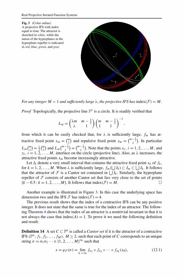
Fig. 3 (Color online)A projective IFS with indexequal to four. The attractor issketched in white, while theunion of the hyperplanes in thehyperplane repeller is indicatedin red, blue, green, and gray

For any integer M > 1 and sufficiently large λ, the projective IFS has index(F ) = M.

Proof Topologically, the projective line P1 is a circle. It is readily verified that

Lm =(

λm m − 12

λ 1

)(m m − 1

21 1

)−1

,

from which it can be easily checked that, for λ is sufficiently large, fm has at-

tractive fixed point xm = (m1

)and repulsive fixed point ym = (m− 1

21

). In particular

Lm

(m1

) = λ2

(m1

)and Lm

(m− 12

1

) = (m− 12

1

). Note that the points xi, i = 1,2, . . . ,M, and

yi, i = 1,2, . . . ,M, interlace on the circle (projective line). Also, as λ increases, theattractive fixed points xm become increasingly attractive.

Let Ik denote a very small interval that contains the attractive fixed point xk of fk ,for k = 1,2, . . . ,M. When λ is sufficiently large, fm(

⋃Ik) ⊂ Im ⊂ ⋃

Ik. It followsthat the attractor of F is a Cantor set contained in

⋃Ik . Similarly, the hyperplane

repeller of F consists of another Cantor set that lies very close to the set of points{k − 0.5 : k = 1,2, . . . ,M}. It follows that index(F ) = M . �

Another example is illustrated in Figure 3. In this case the underlying space hasdimension two and the IFS F has index(F ) = 4.

The previous result shows that the index of a contractive IFS can be any positiveinteger. It does not state that the same is true for the index of an attractor. The follow-ing Theorem 4 shows that the index of an attractor is a nontrivial invariant in that it isnot always the case that index(A) = 1. To prove it we need the following definitionand result.

Definition 14 A set C ⊂ Pn is called a Cantor set if it is the attractor of a contractive

IFS (Pn;f1, f2, . . . , fM), M ≥ 2, such that each point of C corresponds to an uniquestring σ = σ1σ2 · · · ∈ {1,2, . . . ,M}∞ such that

x = ϕF (σ ) = limk→∞fσ1 ◦ fσ2 ◦ · · · ◦ fσk

(x0), (12.1)


where x0 is any point in C.

Lemma 11 Let F = (P n;f1, f2, . . . , fM) be a projective IFS whose attractor is aCantor set C. Let the projective IFS

G = (Pn;fω1, fω2, . . . , fωL)

have the same attractor C, where each fωlis a finite composition of functions in F ,

i.e.,

fωl= fσ l

1◦ fσ l

2◦ · · · ◦ fσ l

jl

in the obvious notation. Then F and G have the same hyperplane repeller andindex(F ) = index(G).

Proof We must show that RG = RF , where RF is the hyperplane repeller of F andRG is the hyperplane repeller of G . Let σ = σ1σ2 · · · and ωl1ωl2 · · · be strings ofsymbols in {1,2, . . . ,M}∞ and {ω1,ω2, . . . ,ωL}∞, respectively. Define

ψ : {ω1,ω2, . . . ,ωL}∞ → {1,2, . . . ,M}∞

by

ψ(ωl1ωl2 · · · ) = ζ(ωl1) ζ(ωl2) · · · where ζ(ωl) = σ l1 σ l

2 · · ·σ ljl.

We claim that ψ is surjective. It is well known that the mapping ϕF :{1,2, . . . ,M}∞ → C in (12.1) is a continuous bijection; see, for example, [2,Chap. 4]. Let σ = σ1σ2 · · · ∈ {1,2, . . . ,M}∞ and let x = limk→∞ fσ1

◦ fσ2 ◦ · · · ◦fσk

(x0). Since C is also the attractor of G it is likewise true that there is at least onestring ω = ωl1ωl2 · · · ∈ {ω1,ω2, . . . ,ωL}∞ such that

x = limk→∞fωl1

◦ fωl2◦ · · · ◦ fωlk

(x0)

= limk→∞(f

σl11

◦ · · · ◦ fσ

l1jl1

) ◦ (fσ

l21

◦ · · · ◦ fσ

l2jl2

) ◦ · · · ◦ (fσ

lk1

◦ · · · ◦ fσ

lkjlk

)(x0).

By the uniqueness of σ in (12.1), we have ψ(ω) = σ , showing that ψ is surjective.We are now going to show that RF ⊆ RG . Let r ∈ RF . Note that the hyperplanes

of P are simply the points of P. Moreover, the hyperplane repeller RF of F is simplythe attractor of the IFS F −1 := (Pn;f −1

1 , f −12 , . . . , f −1

M ) and the hyperplane repeller

RG of G is the attractor of G−1 := (Pn;f −1ω1

, f −1ω2

, . . . , f −1ωL

). Let r0 be the attractivefixed point of f −1

ω1. Note that r0 lies in both RG and in RF . According to Theorems 1

and 3, both F −1 and G−1 are contractive. Therefore

r = limk→∞f −1

σ1◦ f −1

σ2◦ · · · ◦ f −1

σk(r0)

for some σ = σ1σ2 · · · ∈ {1,2, . . . ,M}∞. Since ψ is surjective, there is a stringωl1ωl2 · · · ∈ {ω1,ω2, . . . ,ωL}∞ such that

r = limk→∞f −1

σ1◦ f −1

σ2◦ · · · ◦ f −1

σk(r0)


= limk→∞(f −1

σk◦ fσk−1 ◦ · · · ◦ fσ1)

−1(r0)

= limm→∞(fωlm

◦ fωlm−1◦ · · · ◦ fωl1

)−1(r0)

= limk→∞f −1

ωl1◦ f −1

ωl2◦ · · · ◦ f −1

ωlk(r0) ∈ lim

k→∞(G−1)k(r0) = RG .

A similar, but easier, argument shows that RG ⊆ RF . Hence F and G have the samehyperplane repeller. Since the attractors and hyperplane repellers of both are the samewe have index(F ) = index(G) by the definition of the index. �

Theorem 4 If F = (P1;f1, f2) is the projective IFS in Proposition 12 with M = 2,

λ = 10, and A is the attractor of F , then index(A) = 2.

Proof Let F = (P1; f1, f2), where

f1 =(

110 00 1

)

, f2 =(

37 −1854 −26

)

.

It is easy to check that f1 = f ◦ f1 ◦ f −1 and f2 = f ◦ f2 ◦ f −1 where f1 and f2 arethe functions in Proposition 12 when λ = 10, and f is the projective transformation

represented by the matrix Lf = ( 1 −11 − 1

2

). It is sufficient to show that if A is the attractor

of F , then index(A) = 2. From here on the IFS F is not used, so we drop the “hat”from F , f1, f2, A. Also to simplify notation, the set of points of the projective line aretaken to be P = R ∪ {∞}, where

(x1

)is denoted as the fraction x and

(10

)is denoted

as ∞. In this notation f1(x) = 110x and f2(x) = 37x−18

54x−26 when restricted to R. Thefollowing are properties of F .

(1) The attractor C of F is a Cantor set.(2) index(F ) = 2.(3) The origin a = 0 is the attractive fixed point of f1 while its repulsive hyperplane

is ∞.(4) The attractive fixed point of f2 is at c = 2/3 and its repulsive hyperplane is at

1/2.(5) C ⊂ [a, b] ∪ [c, d], where b = 11

40 − 1120

√609 (= 0.069351) and d = 11

4 −112

√609 (= 0.69351) are the attractive fixed points of f1 ◦ f2 and f2 ◦ f1, re-

spectively.(6) If h is any projective transformation taking C into itself, then h([a, b] ∪ [c, d]) ⊂

[a, b] ∪ [c, d].(7) The symmetry group of C is trivial, i.e., the only projective transformation h such

that h(C) = C is the identity.

Property (1) is in the proof of Proposition 12, and property (2) is a consequenceof Proposition 12. Properties (3) and (4) are easily verified by direct calculation.Property (5) can be verified by checking that F ([a, b] ∪ [c, d]) ⊂ [a, b] ∪ [c, d].

To prove property (6), let I denote a closed interval (on the projective line,topologically a circle) that contains C. Its image h−1(I ) is also a closed inter-val. Since h(C) ⊂ C, it follows that C ⊂ h−1(C). Since C contains {a, b, c, d}


and some points between a and b, h−1(I ) must contain a, b and some points be-tween a and b. It follows that h−1(I ) ⊃ [a, b]. Similarly h−1(I ) ⊃ [c, d]. There-fore h−1(I ) ⊃ [a, b] ∪ [c, d], and hence h([a, b] ∪ [c, d]) ⊂ I . Now choose I tobe [a, d] to get (A) h([a, b] ∪ [c, d]) ⊂ [a, d]. Choose I to be [c, b] (by which wemean the line segment that goes from c through d then ∞ = −∞ then through a toend at b) to obtain (B) h([a, b] ∪ [c, d]) ⊂ [c, b]. It follows from (A) and (B) thath([a, b] ∪ [c, d]) ⊂ [a, d] ∩ [c, b] = [a, b] ∪ [c, d].

To prove property (7), assume that h(C) = C. We will show that h must be theidentity. By property (6) h([a, b] ∪ [c, d]) = [a, b] ∪ [c, d]. Taking the complement,we have h((b, c)∪ (d, a)) = (b, c)∪ (d, a), and so h([b, c] ∪ [d, a]) = [b, c] ∪ [d, a].Hence

h([a, b] ∪ [c, d]) ∩ h([b, c] ∪ [d, a])= ([a, b] ∪ [c, d]) ∩ ([b, c] ∪ [d, a]).

It follows that h({a, b, c, d}) = {a, b, c, d}. Any projective transformation that maps{a, b, c, d} to itself must preserve the cross ratio of the four points, so the only possi-bilities are (i) h(a) = a, h(b) = b, h(c) = c, h(d) = d , in which case h is the identitymap; (ii) h(a) = b, h(b) = a, h(c) = d , h(d) = c; (iii) h(a) = c, h(b) = d , h(c) = a,h(d) = b, and (iv) h(a) = d , h(b) = c, h(c) = b, h(d) = a. In each case one can writedown the specific projective transformation, for example, (iii) is achieved by

h(x) = (d − c)(b − c)(x − a)

(b − a + d − c)(x − c) − (d − c)(b − c)+ c.

The other two specific transformations can be deduced by permuting the symbols a,b, c, d . In each of the cases (ii), (iii), and (iv) it is straightforward to check numericallythat h(x) does not map C into C. (One compares the union of closed intervals

[f1(a), f1(b)] ∪ [f1(c), f1(d)] ∪ [f2(a), f2(b)] ∪ [f2(c), f2(d)],whose endpoints belong to C and which contains C, with the union

[h(f1(a)), h(f1(b))] ∪ [h(f1(c)), h(f1(d))]∪[h(f2(a)), h(f2(b))] ∪ [h(f2(c)), h(f2(d))]).

It follows that h must be the identity map, as claimed.Let G = (P1;g1, g2, . . . , gL) be any projective IFS with attractor equal to C. The

proof proceeds by showing the following: (‡) for any g ∈ G we have g = fσ1 ◦ fσ2 ◦· · · ◦ fσk

, for some k, where each σi is either 1 or 2. Then, by Lemma 11, G has thesame hyperplane repeller as F , and hence index(G) = index(F ) = 2. So any IFS withattractor C has index 2. This completes the proof of Theorem 4 because it shows thatany IFS with attractor C has index 2, i.e., index(C) = 2.

To prove claim (‡), consider the IFS H = ([a, b]∪ [c, d];f1, f2, g) where g is anyfunction in IFS G . By property (6) g([a, b]∪[c, d]) ⊂ [a, b]∪[c, d]. So H is indeed awell-defined IFS. It follows immediately from the fact that both F and G have attrac-tor equal to C that H also has attractor C. It cannot be the case that g([a, b]) ⊂ [a, b]


and g([c, d]) ⊂ [c, d]) since then g would have two attractive fixed points, which isimpossible. Similarly, it cannot occur that g([c, d]) ⊂ [a, b] and g([a, b]) ⊂ [c, d]for then g2 would have two attractive fixed points, which is also impossible. It cannotoccur that g(a) ⊂ [a, b] and g(b) ⊂ [c, d] for then g([a, b] ∪ [c, d]) would not becontained in [a, b] ∪ [c, d], contrary to property (6). Similarly, we rule out the pos-sibilities that g(a) ⊂ [c, d] and g(b) ⊂ [a, b]; that g(c) ⊂ [a, b] and g(d) ⊂ [c, d];and that g(d) ⊂ [a, b] and g(c) ⊂ [c, d]. It follows that either g([a, b] ∪ [c, d]) ⊂[a, b] ⊂ f1([a, d]), or g([a, b]∪ [c, d]) ⊂ [c, d] ⊂ f2([c, b]) where [c, b] denotes theinterval from c to ∞ then from −∞ to b. (Here, the containments [a, b] ⊂ f2([c, b])and [c, d] ⊂ f2([c, b]) are readily verified by direct calculation.) It now follows thateither g(C) ⊂ C ∩ f1([a, d]) = f1(C) or g(C) ⊂ C ∩ f2([c, b]) = f2(C). Hence

g(C) ⊂ Cσ1 := fσ1(C)

for σ1 ∈ {1,2}. If g(C) = Cσ1 then h(C) = C where h is the projective transformationf −1

σ1◦ g. In this case property (7) implies that h must be the identity map. Therefore

g = fσ1 .

If, on the other hand, g(C) � fσ1(C), then we consider the IFS

Hσ1 = (fσ1([a, b] ∪ [c, d]);fσ1 ◦ f1 ◦ f −1σ1

, fσ1 ◦ f2 ◦ f −1σ1

, g ◦ f −1σ1

).

It is readily checked that the functions that comprise this IFS indeed map fσ1([a, b]∪[c, d]) into itself. The attractor of Hσ1 is Cσ1 = fσ1(C) because

Hσ1(Cσ1) = fσ1 ◦ f1 ◦ f −1σ1

(fσ1(C)) ∪ fσ1 ◦ f2 ◦ f −1σ1

(fσ1(C)) ∪ g ◦ f −1σ1

(fσ1(C))

= fσ1(f1(C) ∪ f2(C)) ∪ g(C) = fσ1(C) ∪ g(C)

= Cσ1 (because g(C) ⊂ fσ1(C)).

Let

aσ1 < bσ1 < cσ1 < dσ1

denote the endpoints of the two intervals fσ1([a, b]) and fσ1([c, d]), and write ournew IFS as

Hσ1 = ([aσ1, bσ1] ∪ [cσ1, dσ1];f(σ1)1, f(σ1)2, gσ1),

where

f(σ1)σ2 = fσ1 ◦ fσ2 ◦ f −1σ1

, and gσ1 = g ◦ f −1σ1

.

Repeat our earlier argument to obtain

gσ1([aσ1 , bσ1] ∪ [cσ1, dσ1]) ⊂ fσ2([aσ1, bσ1] ∪ [cσ1, dσ1]),and in particular that

gσ1(Cσ1) ⊂ Cσ1σ2 := f(σ1)σ2(Cσ1) = fσ1 ◦ fσ2 ◦ f −1σ1

◦ fσ1(C) = fσ1 ◦ fσ2(C)


for some σ2 ∈ {1,2}. If gσ1(Cσ1) = Cσ1σ2 then gσ1(fσ1(C)) = fσ1 ◦ fσ2(C) whichimplies g ◦ f −1

σ1◦ fσ1(C) = fσ1 ◦ fσ2(C) which implies, as above, that

g = fσ1 ◦ fσ2 .

If gσ1(Cσ1) � Cσ1σ2 then we construct a new projective IFS Hσ1σ2 in the obvious wayand continue the argument. If the process does not terminate with

g = fσ1 ◦ fσ2 ◦ · · · ◦ fσk

for some k, then g(C) is a singleton, which is impossible because g is invertible. Weconclude that

G = (P;fω1, fω2, . . . , fωL)

where

fωl= fσ l

1◦ fσ l

2◦ · · · ◦ fσ l

kl

in the obvious notation. This concludes the proof of claim (‡).Now Lemma 11 implies index(G) = index(F ). So the index of any projective IFS

that has C as its attractor is 2. It follows that index(A) = 2. �

13 Remarks

Various remarks are placed in this section so as to avoid interrupting the flow of themain development.

Remark 1 Example 3 in Sect. 4 illustrates that there exist non-contractive projectiveIFSs that, nevertheless, have attractors. Such IFSs are not well understood and invitefurther research.

Remark 2 It is well known [27] that if each function of an IFS is a contraction on acomplete metric space X, then F has a unique attractor in X. So statement (4) of theTheorem 1 immediately implies the existence of an attractor A, but not that there is ahyperplane H such that A ∩ H = ∅.

Remark 3 Let F be a contractive IFS. By Corollary 1, each f ∈ F has an invarianthyperplane Hf . If all these invariant hyperplanes are identical, say Hf = H for allf ∈ F , then the projective IFS F is equivalent to an affine IFS acting on the embed-ded affine space P

n\H . More specifically, let G = (Rn;g1, g2, . . . , gM) be an affineIFS where gi(x) = L′

i (x) + ti and where L′i is the linear part and ti the translational

part. A corresponding projective IFS is F = (Pn;f1, f2, . . . , fM) where, for each i

the projective transformation fi is represented by the matrix Lfi:

Lfi

⎛

⎜⎜⎝

x0x1.

xn

⎞

⎟⎟⎠ =

(1 0ti L

′i

)⎛

⎜⎜⎝

x0x1.

xn

⎞

⎟⎟⎠ .


Here Rn corresponds to P\H with H the hyperplane x0 = 0. In this case the hyper-

plane repeller of F is H.

Remark 4 Straightforward geometrical comparisons between dK(x, y) and dP(x, y)

show that (i) the two metrics are bi-Lipschitz equivalent on any convex body con-tained in int(K) and (ii) if f is any projective transformation on P

n then the metricdf (P) defined by df (P)(x, y) = dP(f (x), f (y)) for all x, y ∈ P

n is bi-Lipschitz equiv-alent to dP. A consequence of assertions (i) and (ii) is that the value of the Hausdorffdimension of any compact subset of int(K) is the same if it is computed using theround metric dP or the Hilbert metric dK ; see [20, Corollary 2.4, p. 30], and its valueis invariant under the group of projective transformations on P

n. In particular, theHausdorff dimension of an attractor of a projective IFS is a projective invariant.

Remark 5 Theorem 1 provides conditions for the existence of a metric with respectto which a projective IFS is contractive. In so doing, it invites other directions ofdevelopment, including IFS with place-dependent probabilities [9], graph-directedIFS theory [24], projective fractal interpolation, and so on. In subsequent papers wehope to describe a natural generalization of the joint spectral radius and applicationsto digital imaging.

Remark 6 Definition 2 of the attractor of an IFS is a natural generalization of thedefinition [2, p. 82] of the attractor of a contractive IFS. Another general definition,in the context of iterated closed relations on a compact Hausdorff space, has beengiven by McGehee [25]. He proves that his definition is equivalent to Definition 2,for the case of contractive iterated function systems. However, readily constructedexamples show that McGehee’s definition of attractor is weaker than Definition 2.

Acknowledgements We thank David C. Wilson for many helpful discussions; he influenced the styleand contents of this paper and drew our attention to the Krein–Rutman theorem.

References

1. Atkins, R., Barnsley, M.F., Wilson, D.C., Vince, A.: A characterization of point-fibred affine iteratedfunction systems. Topol. Proc. 38, 189–211 (2010)

2. Barnsley, M.F.: Fractals Everywhere. Academic Press, Boston (1988)3. Barnsley, M.F.: Fractal image compression. Not. Am. Math. Soc. 43, 657–662 (1996)4. Barnsley, M.F.: Introduction to IMA fractal proceedings. In: Fractals in Multimedia, Minneapolis,

MN, 2001. IMA Vol. Math. Appl., vol. 132, pp. 1–12. Springer, New York (2002)5. Barnsley, M.F.: Superfractals. Cambridge University Press, Cambridge (2006)6. Barnsley, M.F.: The life and survival of mathematical ideas. Not. Am. Math. Soc. 57, 12–24 (2010)7. Barnsley, M.F., Demko, S.G.: Iterated function systems and the global construction of fractals. Proc.

R. Soc. Lond., Ser. A 399, 243–275 (1985)8. Barnsley, M.F., Hurd, L.P.: Fractal Image Compression. AK Peters, Wellesley (1993). Illustrations by

Louisa F. Anson9. Barnsley, M.F., Demko, S.G., Elton, J.H., Elton, J.S.: Invariant measures for Markov processes arising

from iterated function systems with place-dependent probabilities. Ann. Inst. Henri Poincaré Probab.Stat. 24, 367–394 (1988)

10. Barnsley, M.F., Hutchinson, J., Stenflo, Ö.: V-variable fractals: fractals with partial self similarity.Adv. Math. 218, 2051–2088 (2008)


11. Berger, M.A.: Random affine iterated function systems: curve generation and wavelets. SIAM Rev.34, 361–385 (1992)

12. Berger, M.A., Wang, Y.: Bounded semigroups of matrices. Linear Algebra Appl. 166, 21–27 (1992)13. Birkhoff, G.: Extensions of Jentzsch’s theorem. Trans. Am. Math. Soc. 85, 219–227 (1957)14. Blanc-Talon, J.: Self-controlled fractal splines for terrain reconstruction. IMACS World Congr. Sci.

Comput. Model. Appl. Math. 114, 185–204 (1997)15. Brualdi, R.A.: Introductory Combinatorics, 4th edn. Elsevier, New York (1997)16. Buseman, H.: The Geometry of Geodesics. Academic Press, New York (1955)17. Bushell, P.J.: Hilbert’s metric and positive contraction mappings in Banach space. Arch. Ration. Mech.

Anal. 52, 330–338.G (1973)18. de Groot, J., de Vries, H.: Convex sets in projective space. Compos. Math. 13, 113–118 (1957)19. Dekker, D.: Convex regions in projective N-space. Am. Math. Mon. 62, 430–431 (1955)20. Falconer, K.: Fractal Geometry: Mathematical Foundations and Applications. Wiley, Chichester

(1990)21. Fisher, Y.: Fractal Image Compression: Theory and Application. Springer, New York (1995)22. Hutchinson, J.E.: Fractals and self-similarity. Indiana Univ. Math. J. 30, 713–747 (1981)23. Krein, M.G., Rutman, M.A.: Linear operators leaving invariant a cone in a Banach space. Translations

American Mathematical Society 26 (1950). Translated from Usp. Mat. Nauk (N.S.) 3(1(23)), 3–95(1948)

24. Mauldin, R.D., Williams, S.C.: Random recursive constructions: asymptotic geometrical and topolog-ical properties. Trans. Am. Math. Soc. 295, 325–346 (1986)

25. McGehee, R.: Attractors for closed relations on compact Hausdorff spaces. Indiana Univ. Math. J. 41,1165–1209 (1992)

26. Shilov, G.E.: Linear Algebra. Dover, Minneola (1997)27. Williams, R.F.: Composition of contractions. Bol. Soc. Bras. Mat. 2, 55–59 (1971)

real projective iterated function systems - people · michael f. barnsley ·andrew vince ... real...

Documents