1

Real-Time Accurate Stereo Matching using

Modified Two-Pass Aggregation and Winner-Take-

All Guided Dynamic Programming

Xuefeng Chang

Beihang University

2011.5.15

2

Back ground

Global Methods

Minimize a certain energy function

Graph-cut，Belief propagation

High accuracy ,Low speed

Local Methods

Aggregate matching cost in a local support window

Winner-Take-All (WTA) Strategy

Fast but inaccurate

Stereo Algorithms

3

Back ground

Locally Adaptive Support-Weight Approach

(Yoon and Kweon CVPR 2005)

A fixed-size support window with per-pixel varying support weight.

The support weight is computed based on color similarity and

geometric distance to the center pixel of interest.

Very good results (Avg. Error 6.67%).

Computationally expensive, off-line.

( , ) exp( ( ))pq pq

c g

C gS p q

r r

,

,

'

,

'

,

( , ) ( , )) ( , )( )

( , ) ( , ))

i ip q

i ip q

i i

d x yp q

d i i

p q

S p p S q q C p pW p

S p p S q q

{ , , }

( , ) | ( , ) ( , ) |x y x y x yccdc r g b

C p p I p p I p d p

4

Back ground

Real-Time Stereo using Adaptive Weight

(Liang Wang 3dpvt2006)

The per-pixel matching cost is only aggregated in a one dimensional vertical window.

The Adaptive weight scheme is integrated into a DP framework.

Achieves over 50 million disparity evaluations per second (MDE/s) when using the graphics hardware.

The quality is not quite satisfactory (Avg. Error 9.82%).

5

Our approach

Framework

Two-Pass Aggregation

Disparity Computation with

WTA guided DP

Maching Cost Computation

6

Weight computation by color similarity

Our Approach

2

{ , , }

( ( , ) ( , )) )(pq c x y c x y

c r g b

C sqrt p p I q qI

( , ) exp( )pq

c

CS p q

r

Only color similarity is used to calculate support weight.

Color Only Color And Distance

7

Our Approach

Two-Pass Aggregation

...

...

computes once,

uses many times

Simplifies the matching cost aggregation process

by multi-use of computational results

O(N2) O(N)

8

Our Approach

( , , , ) ( , , )( , , )

( , , , )

r

r x r

r

x r

w u v u x v C u x v dH u v d

w u v u x v

( , , , ) ( , , )( , , )

( , , , )

r r

y rr

r

x r

w u v u v y H u v y dV u v d

w u v u v y

'( , ) ( ', ) ( , ')S c p S c p S c c' '

'( , ) exp( )pc cc

c

c cS c p

r

( , ) exp( )pc

c

cS c p

r

ApproximateWeight

OriginalWeight

Accuracy loss during two-pass aggregation

p

c

c’

9

c c’

p

c c’

p

c c’ p

c’ cpc c’

p

Our Approach

maxmin

b

..

.c’

c

p

r

g

We can have a clear view of the difference between

S(c,p) and S’(c,p) in Color Space

' ' ' '0 2 min( , )pc cc pc pc ccc c c c

The larger and ,

the larger the possible accuracy loss.'pcc

'cc

10

Our Approach Credibility estimation mechanism

' '

1

2

( , ) (exp( )) (exp( )

0,

( ) 0.5,

1,

pc cc

w

w

c cR c p T T

K K

x T

T x x T

else

Aggregates in a fixed support window(35×35)

Excludes points which may be unreliable

from two-pass aggregation.

Computes a credibility value for each pixel

Without credibility estimation

With credibility estimation

11

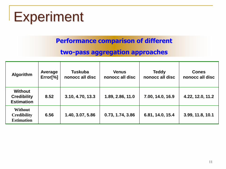
Experiment

Performance comparison of different

two-pass aggregation approaches

AlgorithmAverage

Error[%]

Tuskuba

nonocc all disc

Venus

nonocc all disc

Teddy

nonocc all disc

Cones

nonocc all disc

Without

Credibility

Estimation

8.52 3.10, 4.70, 13.3 1.89, 2.86, 11.0 7.00, 14.0, 16.9 4.22, 12.0, 11.2

Without

Credibility

Estimation

6.56 1.40, 3.07, 5.86 0.73, 1.74, 3.86 6.81, 14.0, 15.4 3.99, 11.8, 10.1

12

Our Approach

Disparity computation with Scan-line DP

Energy Function

Depth

DP

Y

X

D

Width

( ) ( ) ( )data smoothE d E d E d

Smooth

Matching Cost

1

| ( ) ( 1) | *Width

smooth

x

E d x d x

( )data dE W p

For , we only need to consider d(p)-1, d(p), d(p)+1 as

disparity smoothness constrain.

( )[ ( ) 1, ( ), ( ) 1]

( , ( )) ( ) min { ( ', ) * ( ( ) )}d pd d p d p d p

F p d p W p F p d abs d p d

' ( 1, )x yp p p

13

Our Approach

So we adopt a winner-take-all guided dynamic programming.

The 4th candidate disparity

But disparities computed by this method change slowly at

depth discontinue areas, and may blur the borders.

1( )

[ ( ) 1, ( ), ( ) 1, ]( , ( )) ( ) min { ( ', ) * ( ( ) )}

xd p

d d p d p d p dF p d p W p F p d abs d p d

1arg min '( ', )

xd

d C p d

+

DP WTA DP+WTA

14

Experiment

Performance comparison of different

disparity computation method

AlgorithmAverage

Error[%]

Tuskuba

nonocc all disc

Venus

nonocc all disc

Teddy

nonocc all disc

Cones

nonocc all disc

DP 7.27 1.54, 3.30, 6.68 0.79, 1.95, 5.15 6.89, 14.2, 15.6 5.02, 13.1, 13.0

WTA 9.32 3.20, 5.21, 7.04 2.49, 3.93, 9.66 10.3, 18.0, 18.5 5.92, 15.4, 12.2

DP+WTA 6.56 1.40, 3.07, 5.86 0.73, 1.74, 3.86 6.81, 14.0, 15.4 3.99, 11.8, 10.1

15

Experiment

Resulting depth maps from Middlebury stereo data set

AlgorithmAverage

Error[%]

Tuskuba

nonocc all disc

Venus

nonocc all disc

Teddy

nonocc all disc

Cones

nonocc all disc

Our approach 6.56 1.40, 3.07, 5.86 0.73, 1.74, 3.86 6.81, 14.0, 15.4 3.99, 11.8, 10.1

Adaptive Weight 6.67 1.38, 1.85, 6.90 0.71, 1.19, 6.13 7.88, 13.3, 18.6 3.97, 9.79, 8.26

RealTimeABW 7.90 1.26, 1.67, 6.83 0.33, 0.65, 3.56 10.7, 18.3, 23.3 4.81, 12.6, 10.7

RealTimeBP 7.69 1.49, 3.40, 7.87 0.77, 1.90, 9.00 7.78, 14.9, 17.3, 4.58, 12.4, 10.7

RTCensus 9.73 5.08, 6.25, 19.2 1.58, 2.42, 14.2 7.96, 13.8, 20.3 4.10, 9.54, 12.2

Real-Time GPU 9.82 2.05, 4.22, 10.6 1.92, 2.98, 20.3 7.23, 14.4, 17.6 6.41, 13.7, 16.5

16

ExperimentExperiment on dynamic scene

Speed: 20 fps on 320×240 video with GPU acceleration

(disparity search range =24)

17

Thank you!

Q&A