San Jose State University San Jose State University

SJSU ScholarWorks SJSU ScholarWorks

Master's Projects Master's Theses and Graduate Research

Spring 5-18-2020

REAL-TIME AD CLICK FRAUD DETECTION REAL-TIME AD CLICK FRAUD DETECTION

Apoorva Srivastava San Jose State University

Follow this and additional works at: https://scholarworks.sjsu.edu/etd_projects

Part of the Artificial Intelligence and Robotics Commons, and the Information Security Commons

Recommended Citation Recommended Citation Srivastava, Apoorva, "REAL-TIME AD CLICK FRAUD DETECTION" (2020). Master's Projects. 916. DOI: https://doi.org/10.31979/etd.gthc-k85g https://scholarworks.sjsu.edu/etd_projects/916

This Master's Project is brought to you for free and open access by the Master's Theses and Graduate Research at SJSU ScholarWorks. It has been accepted for inclusion in Master's Projects by an authorized administrator of SJSU ScholarWorks. For more information, please contact scholarworks@sjsu.edu.

REAL-TIME AD CLICK FRAUD DETECTION

A Thesis

Presented to

The Faculty of the Department of Computer Science

San Jose State University

In Partial Fulfillment

of the Requirements for the Degree

Master of Science

by

Apoorva Srivastava

May 2020

© 2020

Apoorva Srivastava

ALL RIGHTS RESERVED

The Designated Thesis Committee Approves the Thesis Titled

REAL-TIME AD CLICK FRAUD DETECTION

by

Apoorva Srivastava

APPROVED FOR THE DEPARTMENT OF COMPUTER SCIENCE

SAN JOSE STATE UNIVERSITY

May 2020

Dr. Robert Chun, Ph.D. Department of Computer Science

Dr. Thomas Austin, Ph.D. Department of Computer Science

Shobhit Saxena Google LLC

ABSTRACT

REAL-TIME AD CLICK FRAUD DETECTION

by Apoorva Srivastava

With the increase in Internet usage, it is now considered a very important platform for

advertising and marketing. Digital marketing has become very important to the economy:

some of the major Internet services available publicly to users are free, thanks to digital

advertising. It has also allowed the publisher ecosystem to flourish, ensuring significant

monetary incentives for creating quality public content, helping to usher in the

information age. Digital advertising, however, comes with its own set of challenges. One

of the biggest challenges is ad fraud. There is a proliferation of malicious parties and

software seeking to undermine the ecosystem and causing monetary harm to digital

advertisers and ad networks. Pay-per-click advertising is especially susceptible to click

fraud, where each click is highly valuable. This leads advertisers to lose money and ad

networks to lose their credibility, hurting the overall ecosystem. Much of the fraud

detection is done in offline data pipelines, which compute fraud/non-fraud labels on clicks

long after they happened. This is because click fraud detection usually depends on

complex machine learning models using a large number of features on huge datasets,

which can be very costly to train and lookup. In this thesis, the existence of low-cost ad

click fraud classifiers with reasonable precision and recall is hypothesized. A set of

simple heuristics as well as basic machine learning models (with associated simplified

feature spaces) are compared with complex machine learning models, on performance and

classification accuracy. Through research and experimentation, a performant classifier is

discovered which can be deployed for real-time fraud detection.

Keywords – Digital marketing, Online advertising, Click fraud detection, Ad

Spam, Real-time fraud detection

ACKNOWLEDGMENTS

I would like to thank my advisor, Prof. Chun for providing critical advice and helped

me navigate through this complex project. Without his guidance and blessings, this

project and thesis would not have been possible.

I would also like to thank my family. Without their support, I would have never been

able to complete this thesis or pursue my dreams.

v

TABLE OF CONTENTS

List of Tables . . . . . . . . . . . . . . . . . . . . . . . . . . . . . . . . . . . . . . . . . . . . . . . . . . . . . . . . . . . . . . . . . . . . . . . . . . viii

List of Figures . . . . . . . . . . . . . . . . . . . . . . . . . . . . . . . . . . . . . . . . . . . . . . . . . . . . . . . . . . . . . . . . . . . . . . . . . ix

1 Introduction. . . . . . . . . . . . . . . . . . . . . . . . . . . . . . . . . . . . . . . . . . . . . . . . . . . . . . . . . . . . . . . . . . . . . . . . 1

2 Literature Survey . . . . . . . . . . . . . . . . . . . . . . . . . . . . . . . . . . . . . . . . . . . . . . . . . . . . . . . . . . . . . . . . . . 62.1 Logged-events Based Approaches . . . . . . . . . . . . . . . . . . . . . . . . . . . . . . . . . . . . . . . 62.2 Client-based Approaches . . . . . . . . . . . . . . . . . . . . . . . . . . . . . . . . . . . . . . . . . . . . . . . . . 14

3 Datasets . . . . . . . . . . . . . . . . . . . . . . . . . . . . . . . . . . . . . . . . . . . . . . . . . . . . . . . . . . . . . . . . . . . . . . . . . . . . 163.1 Original datasets . . . . . . . . . . . . . . . . . . . . . . . . . . . . . . . . . . . . . . . . . . . . . . . . . . . . . . . . . . 163.2 Construction. . . . . . . . . . . . . . . . . . . . . . . . . . . . . . . . . . . . . . . . . . . . . . . . . . . . . . . . . . . . . . . 163.3 Dataset hosting . . . . . . . . . . . . . . . . . . . . . . . . . . . . . . . . . . . . . . . . . . . . . . . . . . . . . . . . . . . . 17

4 Exploratory Data Analysis . . . . . . . . . . . . . . . . . . . . . . . . . . . . . . . . . . . . . . . . . . . . . . . . . . . . . . . 204.1 Conversion Sparsity . . . . . . . . . . . . . . . . . . . . . . . . . . . . . . . . . . . . . . . . . . . . . . . . . . . . . . 204.2 Clicky IPs . . . . . . . . . . . . . . . . . . . . . . . . . . . . . . . . . . . . . . . . . . . . . . . . . . . . . . . . . . . . . . . . . 214.3 Relationship between #Clicks and Conversion Rates. . . . . . . . . . . . . . . . . . . 214.4 Apps and Conversion Rates . . . . . . . . . . . . . . . . . . . . . . . . . . . . . . . . . . . . . . . . . . . . . . 224.5 Conversion Rates by Device Types . . . . . . . . . . . . . . . . . . . . . . . . . . . . . . . . . . . . . . 234.6 Channel Conversion Rates . . . . . . . . . . . . . . . . . . . . . . . . . . . . . . . . . . . . . . . . . . . . . . . 254.7 Conversion Rate Time Series . . . . . . . . . . . . . . . . . . . . . . . . . . . . . . . . . . . . . . . . . . . . 25

5 System Design . . . . . . . . . . . . . . . . . . . . . . . . . . . . . . . . . . . . . . . . . . . . . . . . . . . . . . . . . . . . . . . . . . . . 27

6 Multi-Level Perceptrons . . . . . . . . . . . . . . . . . . . . . . . . . . . . . . . . . . . . . . . . . . . . . . . . . . . . . . . . . . 296.1 MLP Construction . . . . . . . . . . . . . . . . . . . . . . . . . . . . . . . . . . . . . . . . . . . . . . . . . . . . . . . . 296.2 Performance . . . . . . . . . . . . . . . . . . . . . . . . . . . . . . . . . . . . . . . . . . . . . . . . . . . . . . . . . . . . . . . 30

7 Heuristics . . . . . . . . . . . . . . . . . . . . . . . . . . . . . . . . . . . . . . . . . . . . . . . . . . . . . . . . . . . . . . . . . . . . . . . . . . 327.1 Sessionization . . . . . . . . . . . . . . . . . . . . . . . . . . . . . . . . . . . . . . . . . . . . . . . . . . . . . . . . . . . . . 327.2 Heuristics Explored . . . . . . . . . . . . . . . . . . . . . . . . . . . . . . . . . . . . . . . . . . . . . . . . . . . . . . . 33

7.2.1 High attribute conversion rate . . . . . . . . . . . . . . . . . . . . . . . . . . . . . . . . . . . . . . 337.2.2 IP's clicks too high in an hour. . . . . . . . . . . . . . . . . . . . . . . . . . . . . . . . . . . . . . 337.2.3 Session's last click is convertible. . . . . . . . . . . . . . . . . . . . . . . . . . . . . . . . . . . 34

7.3 Heuristic Combination . . . . . . . . . . . . . . . . . . . . . . . . . . . . . . . . . . . . . . . . . . . . . . . . . . . 347.4 Heuristic Results . . . . . . . . . . . . . . . . . . . . . . . . . . . . . . . . . . . . . . . . . . . . . . . . . . . . . . . . . . 34

8 Machine Learning Models . . . . . . . . . . . . . . . . . . . . . . . . . . . . . . . . . . . . . . . . . . . . . . . . . . . . . . . . 37

vi

8.1 Features. . . . . . . . . . . . . . . . . . . . . . . . . . . . . . . . . . . . . . . . . . . . . . . . . . . . . . . . . . . . . . . . . . . . 378.1.1 Feature Descriptions . . . . . . . . . . . . . . . . . . . . . . . . . . . . . . . . . . . . . . . . . . . . . . . . 37

8.2 Base Models . . . . . . . . . . . . . . . . . . . . . . . . . . . . . . . . . . . . . . . . . . . . . . . . . . . . . . . . . . . . . . 398.3 One-hot Encoded Feature Space . . . . . . . . . . . . . . . . . . . . . . . . . . . . . . . . . . . . . . . . . 408.4 CvR Space . . . . . . . . . . . . . . . . . . . . . . . . . . . . . . . . . . . . . . . . . . . . . . . . . . . . . . . . . . . . . . . . 438.5 IP Aggregate Features . . . . . . . . . . . . . . . . . . . . . . . . . . . . . . . . . . . . . . . . . . . . . . . . . . . . 45

9 Results . . . . . . . . . . . . . . . . . . . . . . . . . . . . . . . . . . . . . . . . . . . . . . . . . . . . . . . . . . . . . . . . . . . . . . . . . . . . . 47

10 Conclusions and Future Work . . . . . . . . . . . . . . . . . . . . . . . . . . . . . . . . . . . . . . . . . . . . . . . . . . . . 49

Literature Cited . . . . . . . . . . . . . . . . . . . . . . . . . . . . . . . . . . . . . . . . . . . . . . . . . . . . . . . . . . . . . . . . . . . . . . . . 51

vii

viii

LIST OF TABLES

Table 1. Performance Characteristics in Surveyed Literature . . . . . . . . . . . . . . . . . . 13

Table 2. TalkingData Training Data CSV Schema . . . . . . . . . . . . . . . . . . . . . . . . . . . . . . 16

Table 3. Clicky IP Addresses (with #clicks≥ 100) vs. Non-Clicky IPs . . . . . . . 21

Table 4. Multi-Level Perceptrons’ Performance . . . . . . . . . . . . . . . . . . . . . . . . . . . . . . . . . 30

Table 5. Heuristics’ Performance. . . . . . . . . . . . . . . . . . . . . . . . . . . . . . . . . . . . . . . . . . . . . . . . . 35

Table 6. Machine Learning Model Features . . . . . . . . . . . . . . . . . . . . . . . . . . . . . . . . . . . . . 38

Table 7. Base Models’ Performance . . . . . . . . . . . . . . . . . . . . . . . . . . . . . . . . . . . . . . . . . . . . . 39

Table 8. One-hot Models’ Performance . . . . . . . . . . . . . . . . . . . . . . . . . . . . . . . . . . . . . . . . . . 41

Table 9. Models’ Performance in Conversion-Rate Space . . . . . . . . . . . . . . . . . . . . . . 44

Table 10. Models’ Performance with IP Aggregate Features . . . . . . . . . . . . . . . . . . . . 46

ix

LIST OF FIGURES

Fig. 1. The Advertising Ecosystem [2] . . . . . . . . . . . . . . . . . . . . . . . . . . . . . . . . . . . . . . . . . . 2

Fig. 2. Survey Section Organization . . . . . . . . . . . . . . . . . . . . . . . . . . . . . . . . . . . . . . . . . . . . . 6

Fig. 3. Click Concentricity helping identify Ad Fraud [3]. . . . . . . . . . . . . . . . . . . . . . 7

Fig. 4. Data Collection Setup from Kantardzic et. al. [15]. . . . . . . . . . . . . . . . . . . . . . 15

Fig. 5. Dataset Construction. . . . . . . . . . . . . . . . . . . . . . . . . . . . . . . . . . . . . . . . . . . . . . . . . . . . . . 17

Fig. 6. IPs’ Conversion Rates by Number of Clicks.. . . . . . . . . . . . . . . . . . . . . . . . . . . . 22

Fig. 7. Conversion Rates for Various App Ids. . . . . . . . . . . . . . . . . . . . . . . . . . . . . . . . . . . 23

Fig. 8. Conversion Rates for Various OS Ids. . . . . . . . . . . . . . . . . . . . . . . . . . . . . . . . . . . . 24

Fig. 9. Histogram of Conversion Rates Across Various Devices (with clicks≥100) . . . . . . . . . . . . . . . . . . . . . . . . . . . . . . . . . . . . . . . . . . . . . . . . . . . . . . . . . . . . . . . . . . . . . . . . 24

Fig. 10. % of Conversions in Channels Against the Channel CvRs . . . . . . . . . . . . . 25

Fig. 11. Conversion Rate Time Series . . . . . . . . . . . . . . . . . . . . . . . . . . . . . . . . . . . . . . . . . . . . . 26

Fig. 12. System Design. . . . . . . . . . . . . . . . . . . . . . . . . . . . . . . . . . . . . . . . . . . . . . . . . . . . . . . . . . . . . 27

1 INTRODUCTION

In the past few decades, the use of the Internet has grown exponentially. The growth

of the web-based online advertising industry has created many new opportunities for lead

generation, brand awareness, and electronic commerce for advertisers. A large volume of

this content is offered for free. This is true even for content that we used to pay for, such

as newspapers, blogs, advertiser's site (Macy's etc.). Naturally, content creators need to

make up for the absence of income by finding a new revenue stream. This revenue stream

is Internet advertising. By showing relevant ads to their visitors, and having them click on

those ads, content creators are able to convert traffic into an effective revenue stream,

while also delivering value to the users. In the online marketplace, page views, forms

submissions and clicks often result in money changing hands between advertisers, ad

networks, and web site publishers. Figure 1 shows an advertising ecosystem, with various

entities and their relationships. Online advertising has become the greatest source of

revenue for many Internet giants such as Google, Yahoo!, Bing, Facebook, Twitter, etc [1].

These search engines and content destinations make revenue by selling ad views and ad

clicks, which are generated along with the search results or presented alongside their

content.

Digital advertising can be broadly categorized into two types: brand advertising and

performance advertising. In brand advertising, a marketer is essentially looking to

promote their brand by reaching a broad audience. Even before the advent of digital

marketing, brand advertising has been the dominant form of advertising on non-digital

channels, such as Television, Print Media, billboards and hoardings. In this form of

advertising, the views matter, as the advertisers are trying to reach as many users as

possible in their given marketing budget. The pricing models for brand advertising are

predominantly pay-per-view, where the advertisers are charged each time a user views

their ad online. Facebook Ads is a great example of a brand advertising ad network.

1

Fig. 1: The Advertising Ecosystem [2]

In performance advertising, a marketer is trying to drive an outcome: such as online

shopping purchases from their website or offline purchases from their physical stores,

lead generation to create a pool of high-value users, mobile App downloads, etc.

Performance advertising tends to be highly targeted and relatively more contextually

useful to the users. In this form of advertising, the advertisers are typically unwilling to

pay for each ad view, since brand creation and propagation is not the intent, performance

is. Thus, performance advertising tends to use a pay-per-click (PPC) model for pricing,

where advertisers pay for each ad click on the publishers'websites. Google Search Ads is

a great example of a performance advertising network. Other search engines such as

Yahooand Bing also offer performance advertising and pay-per-click pricing. These

search engines take the mantle of matching a user's search terms to the right ads (aka

relevance), and then charge for each ad click.

2

Both these forms of digital advertising are susceptible to ad fraud. In brand

advertising, the predominant ad fraud that occurs is the impression fraud. This is

particularly true of ad networks such as Facebook Ad Network (FAN) or Google Display

Network which place ads on third-party publisher websites (say random

blog.blogwebsite.com). Here, malicious publishers try to garner fraudulent ad

impressions.

In performance advertising, the predominant ad fraud is the click fraud. In this fraud,

malicious players try to generate fraudulent ad clicks, thereby leading the ad network to

charge the advertiser incorrectly. Fraudsters also seek to take advantage of new

opportunities to conduct fraud against these parties with the hope of having some money

illegitimately change into their own hands. Generation of such invalid clicks, either by

humans or software with the intention to make money or to deplete a competitor's budget,

is known as click fraud. This ultimately threatens the fundamental economics of online

advertising, as advertisers are forced off of auctions, and in general, good content can no

longer be supported by advertising. Combating Click Fraud requires significant

investment in resources and large-scale detection systems, as click fraud bots constantly

change and evolve in response to detection.

Click fraud is very demotivating for advertisers. Click fraud drives up advertising

costs for the businesses [2]. It skews the statistics and analytical data the advertisers rely

on to make effective marketing decisions. These decisions could include things such as

which search keywords to bid for ads on, which campaigns to run longer due to a better

return on investment, how much marketing budget should be spent on digital marketing.

The vast majority of click fraud originates from an advertiser's competitors. Click

fraud can help the competitors waste an advertiser's pay-per-click marketing budget, thus

3

driving up their marketing costs (cost per sale / acquisition – CPA). Many ad networks

allow setting daily ad budget upper limits and caps, which means that click fraud can lead

to the daily budget being exhausted and the advertiser's ads stopping altogether. In an

auction scenario, this can in turn reduce the advertising costs for the competitors, as they

do not need to outbid the advertiser in question. Webmasters and publishers are the next

big source of origin for ad click fraud. These publishers have an incentive to click on ads

on their website to generate short-term income, at the cost of advertisers. Fraud rings are

also an important and growing source of ad click fraud. These large groups of people

specifically target certain ad networks to generate large amounts of revenue for themselves.

They might use human click farms, or a huge array of automated programs and botnets.

A wide variety of research has been carried out on this highly sensitive and lucrative

topic. Major ad networks have dedicated research teams which have looked into this

problem. Broadly speaking, the approaches can be classified as logged-event-based (prior

activity information) and client-side based (blocking malware on legitimate

users'machines).

Most of the approaches in use today perform an offline classification of ad click fraud.

Fraud detection usually relies on complex machine learning models, working in

high-dimensional feature spaces. Additionally, the data sets tend to be massive. Big ad

companies might see multiple hundreds of millions of ad clicks per day. Thus, training

these models and using these models for lookups tends to be quite costly. As a result, ad

click fraud is predominantly done offline. This, however, limits the ad networks’ or

advertisers’ response. If the fraud could be detected in real-time, ad networks and

advertisers could be better positioned to investigate the perpetrators and take active

measures.

4

In addition, there is a bigger set of raw features available in real-time. Most ad

companies limit the amount and nature of data they log for each click. This has to do with

their users’ privacy and data retention policies. For instance, many HTTP headers might

not be logged, or IP addresses anonymized before logging. As a result, machine learning

models that could be built offline work with a subset of available data. If the fraud model

training and lookups could be done in real-time, while processing the clicks, there is a

greater possibility of detecting fraud clicks which might be undiscoverable offline.

Unfortunately, most techniques used today typically do not have this level of performance.

There is also a trade-off between fraud model performance versus precision and recall.

It is easy to build models with very low cost, but these would typically suffer from poor

precision and/or recall. A fraud detection system which appropriately optimizes for low

cost, while delivering good precision and recall is highly desirable. This is the subject of

this thesis.

This report details the research and analysis work for real-time ad click fraud

detection. It starts with a literature survey of the state-of-the-art of ad fraud detection, in

section 2. The survey provides an overview of the techniques used for detecting fraud,

along with the performance, wherever mentioned in the associated literature. This is

followed by a description of datasets used for research and experimentation, as well as the

associated dataset construction in section 3. A detailed exploratory data analysis has been

carried out and articulated in section 4. The training and testing system design has been

discussed in section 5. A state of the art model based on multi-level perceptrons is

presented in section 6 as the baseline. Heuristic rules have been explored in section 7.

Following that, machine learning models and associated features are presented in

section 8. The results of various models are presented in section 9. Finally, conclusions

and potential future work have been discussed in section 10.

5

2 LITERATURE SURVEY

This section presents a survey of published papers in reputed journals and conference

proceedings on the topic of ad click fraud detection. There are a wide variety of ad click

fraud detection methods proposed in prior work. This section examines the results and

success these methods have exhibited.

The section is organized as shown in Fig 2. Section 2.1 will analyze the research done

for logged data-based approach. This will consider logged event activity related to ad

network events, advertiser website events and publisher events. Section 2.2 will describe

the studies done on client-based mitigation.

Fig. 2: Survey Section Organization

2.1 Logged-events Based Approaches

A large number of published works use what could be broadly characterized as

logged-events based approaches. The basic idea here is to keep detailed ad impressions,

ad clicks and advertiser website visit logs, and identify or learn patterns signifying

malicious ad clicks.

As one of the earliest works on ad click fraud detection, Li Chen et. al. [3] focused on

crowd-sourcing click fraud attacks. In this scheme, a malicious party sources a set of bad

actors who could be paid to click on ads on a given publisher website, or ads of a

6

particular advertiser across publishers. Li Chen et. al. performed a clustering analysis to

detect crowdsourcing click frauds. Their approach uses multiple click descriptors such as

ClickID, UserIP, SearchQuery, Cookies, AdvertiserID, ClickTime and

so on. They concluded that specific advertisers get predominantly targeted by such

attackers. They also found out that IP addresses are a good identity mechanism to identify

malicious clickers. They defined crowdsourcing fraud click behavior based on 1)

Denseness, 2) Moderateness and 3) Concentricity.

Fig. 3: Click Concentricity helping identify Ad Fraud [3].

Denseness pertains to the entropy between AdvertiserId and UserIP. If, for

example, few IP addresses account for a large share of a given advertiser’s clicks, there’s

a denseness concern indicative of ad click fraud. Similarly, fraudulent ad clicks from

crowdsourcing tend to occur during short time periods, as opposed to regular users’ traffic.

Thus, if the data shows a large number of clicks in a short time duration out of the

ordinary, the data demonstrates a concentricity pattern and is indicative of ad click fraud.

7

Based on these features, the study uses clustering analysis to detect click fraud. For this

clustering, Li Chen et. al. [3] used a bipartite graph between AdvertiserId and

UserIP, and detected groups of IPs deemed to pertain to the fraud operation. Members

in a malicious group click the same advertisers’ ads over a short time period. The model

leveraged this property and can effectively detect the these malicious cliques. On

simulated data sets, Li Chen et. al. have demonstrated 65% to nearly 100% recall, along

with 82% precision on detecting crowdsourcing click fraud on simulated data sets [3].

Additionally, their technique could label 398 million records in 61 minutes, thus incurring

a cost of 9.196 µs per classification.

Matthieu Faou et. al. [4] used a remarkably different approach to combat ad click

spam. They monitored the activities of an ad clicking malware over multiple months, and

created a map of fraudulent actors involved in the malicious activity. They identified these

actors using social network analysis, and then asserted these actors could be pressured

and influenced to disrupt the click fraud emanating from them. To identify these actors,

Faou et. al. analyzed the ad click redirect chains deeply, looking at referrer URLs. They

studied the redirection chains emanating from infected computers, to understand the value

chains and actors’ relationships in real world. With this analysis, they were able to create

a social graph among the actors and to determine the key actors ripe for disrupting the

malware. The study shows that fraud perpetration tends to be concentrated to a few actors.

As such, if these actors could be disrupted, their impact could be significantly curtailed.

Such an approach is good from a long-term perspective. Referral URLs and request

origins, however, could be good signals useful for real-time fraud detection.

Brendan Kitts et. al. [5] proposed a different approach. They used bot signatures for

click fraud detection. They mention that typical ecosystem measures such as Spiders List,

IAB Robots and public domain IP blacklists are insufficient to combat sophisticated bots

perpetrating ad click fraud. Their work recommends creating a common pool of bot

8

signatures. A bot signature is defined as a set of logged HTTP headers corresponding to

the weblog (sequence of requests received) of a service under attack where the bot has

been identified positively, along with the probability of each request originating from that

bot.

According to the study, bot signatures have multiple benefits: (a) They are readily

sharable between security organizations, enabling quicker mitigation of click fraud threats.

(b) They create a good dataset for Ad Networks to test and evaluate their safety systems,

and (c) They allow companies to use labeled data to ensure that their system is accurately

detecting fraudulent traffic. Brendan Kitts et. al. [5] used techniques for creating 8

simulated bots, which create simulated fraudulent traffic of various kinds. They used

different algorithms, such as user click frequency, presence of cookie, IP blacklist, cluster

of users, user ad clicks sequence count, user keyword clicks count for bot filtration.

Frequency capping as a mitigation mechanism (and correspondingly, number of clicks per

IP as a feature) works well. Mature bots, however, were able to circumvent detection and

prevention despite these frequency capping filters. Hence, they trained a decision tree to

utilize multiple features in order to determine whether the traffic is from a bot or from a

human.

The approach by Mehmed Kantardzic et. al. [6] uses multi-model evidence fusion for

detecting click fraud in real-time. The basic idea is to rely on multiple sensors indicative

of ad click fraud, and then fuse the signals from them to make a higher accuracy

detection. The paper identifies each independent sensor component as a data mining

module. Each of these sensors yield identification signals of low precision. The output of

these sensors is then fused and correlated, to achieve better precision. Fusing the data lets

it provide complete and timely assessments of situations and threats, as well as their

significance. They’ve termed their system as a collaborative click fraud detection and

prevention (CCFDP) system. Three modules have been used to find fraudulent clicks.

9

There is (1) a rule/heuristics based module, (2) a click map module, and (3) an outlier

detection module. The sensors span across server as well as client side. Each click is first

scored independently by each module. Scores are later combined using the

Dempster-Shafer evidence theory [7]. The results of the analysis estimated the average

precision of identifying click fraud as 64%. This is despite the fact that there was only

53% highest average precision among the individual modules. The paper has not

discussed performance characteristics associated with the CCFDP system. Given that it is

combining scores across a few weak classifiers, it is expected that the CPU-time would be

reasonably low.

Haitao Xu et. al. [8] have proposed an approach that enables advertisers to detect the

ad click spam at their end, instead of relying on ad networks to filter out such information.

This helps the advertisers evaluate the ad campaign ROI better. In their system, each click

is classified as either fraudulent, casual, or valid. The technical basis of their work is

passively scrutinizing user engagement on the advertisers’ websites and identifying

visiting clients as true users. Haitao Xu et. al. [8] recommended a click fraud detection

system with two components: (1) a proactive functionality test and (2) a passive

examination of browsing behavior. The functionality test is used to check if the client is

authentic (a browser or a bot). It assumes that most clickbots have limited capabilities and

functionality, when compared to regular browsers. For instance, a bot might not be able to

set some cookie, or a value in browswer local-storage. When a device fails the

functionality test, all the clicks originating from that device would be considered

fraudulent. The second component uses browsing behavior to identify if the user is human

or bot. For instance, a bot would likely not engage in a human-like behavior of checking

out various products on an e-marketing website after an ad click. When both these checks

pass, the corresponding click is validated. They have also proposed the concept of a

“casual click”. A casual click is defined as a click done by a real user, with no intention of

10

making a transaction on the advertiser website. If the device passes the functionality test,

but doesn’t show much engagement on the advertiser website, it is marked as a “casual

click”. To test the proposed system, they built a prototype and deployed it on a large

production web server at an advertiser. They ran ad campaigns at a major ad network for

10 days. Their experimental results show that the approach can detect much more

fraudulent clicks than the ad network’s in-house detection system. On an independent

dataset, they demonstrated a 93.9% precision and 94.6% recall. The detection is based on

firing an ajax request with a challenge code for Javascript. Theey observed an average

round-trip time of 200 ms at the clients’ end to facilitate this.

Research done by D. Antoniou et. al. [9] extends the concept of click fraud. They

characterized ad click fraud as a pattern or sequence of ad clicks aimed towards changing

the regular function of a website, with a goal to produce some specific results. The paper

focuses on two types of ad click frauds: 1) Inflationary click fraud: publishers clicking on

ads on their own websites, and 2) Competitive click fraud: advertisers clicking on

competitors’ ads to exhaust their budgets and bring their ROI down. The paper proposed

an algorithm that uses splay trees for: a) tracking publisher web pages, to detect which

web pages encounter bursts using visit frequency, and b) tracking actors’ IPs, to determine

which ones might be malicious, based on their click frequency. The proposed solution in

the paper attempts an real-time click fraud detection using efficient data structures. Their

paper hasn’t discussed the performance characteristics, however, aside from asymptotic

complexities.

One of the first works on an advanced malicious CloudBot detection is done by Yu

Guo et. al. [10]. They used raw traffic analysis to study the CloudBot traffic. Their

detection approach is based on using machine learning techniques with multi-layer

features. They divided the work into three segments. Firstly, a sampling method is

followed to sample across IP and time, and arrive at a more practically viable smaller

11

dataset sample. With this, they were able to extract user characteristics over a significantly

large period of time, while making sure there is sufficient information to identify

cloudbots. Secondly, they used multi-layer traffic features, to encompass the primary

differences between human traffic and cloudbots. Lastly, a method is used for detecting

CloudBots accurately in close to real-time. The feature set suggested in the paper includes

basic features, such as the #peer nodes, #packets, #bytes, #flows, their statistical

characteristics, OS fingerprint information, network packet TTL related features, port

related and application layer features. The models are then evaluated by measuring the

precision (P) and recall (R) rates of identifying IPs belonging to cloud bots. Based on the

experiments, Random Forest models outperform other algorithms, with a high precision

of 93.3%, along with a 94.3% recall. Decision-tree gives the second best results and

logistic regression is the next best algorithm. The results show that Random Forest based

detection methods can provide good classification characteristics. The performance

characteristics haven’t been discussed in the paper.

Riwa Mouawi et. al. [11] proposed a profoundly different approach. The fraud

detection is typically carried out by trust services managed either by the ad networks or

by the advertisers. Typically, there is no collaboration between the two sides. Both the

parties have different interests, sometimes at loggerheads with each other. Riwa Mouawi

et. al. [11] recommend a neutral third party, trusted by both sides, to overcome this

problem. They crowd-sourced data from various (network, publisher, advertiser) triplets

and combined the data across these. 1) Per-publisher % of duration-suspicious clicks, 2)

Per-publisher #Clicks, 3) Per-publisher #UniqueIPs / #Clicks, 4) #Conversions/#Clicks

per-publisher, 5) Time-Variance of #Clicks.

Multiple different machine learning classifiers were tried out: Artificial Neural

Network (ANN) classification, K-nearest Neighbours (KNN) classification and Support

Vector Machine (SVM) classification. In their evaluations, KNN performed the best with

12

98% precision. SVM was the next best classifier, with nearly 96% precision, and it was

followed by ANN with nearly 93% accuracy. Their fraud detection classifiers had a small

false positive rate.

Leyi Song et. al. [12] developed a three stage click detection / click spam filtration

system, on large scale data. The stage-wise filtering system architecture described in this

paper has three major components of the research: 1) Stage 1 consists of heuristics-based

filters to detect the most obvious invalid clicks with very high confidence. These filters

identify the most obvious malicious players: heavy hitters and frequent clickers; 2) Stage

2 consists of classification-based filters. It determines more complex clicks and uses a

labeled training set, and 3) Stage 3 consists of a clustering-based filter, to identify groups

of similar publisher websites involved in malicious behavior. The research analyzed

distance between cluster centroids and diversity in queries to segment malicious groups.

They observed that there is a greater diversity in queries from normal clicks, compared to

the ones originating in malicious groups. Song et. al. [12] presented their results to a

group of ad click fraud experts, and claimed a 97% click-fraud prediction precision.

Table 1: Performance Characteristics in Surveyed Literature

Reference Precision Recall Prediction Time[3] 0.82 9.1959 µs[6] 0.64[8] 0.939 0.946 200 ms (client-side)[11] 0.98[12] 0.976 337 µs

Table 1 summarizes the performance characteristics from reviewed literature. This

summary establishes that machine learning approaches tend to have better precision

characteristics. Additionally, the CPU-time for classification varies widely, depending on

the technique. Even for server-side approaches, the fraud classification could easily

consume upto hundreds of microseconds. While per-request this might look small, this

13

adds up to a lot of compute cost and resources in real-world scenarios, which might deal

with huge number of queries per second. As a result, much of the practical deployments

tend to be offline.

2.2 Client-based Approaches

There are other researchers who have taken the route of identifying the ad-click fraud

right at the source, as opposed to looking through logged events at the ad service, or the

advertiser website. The overall approach is to identify and mitigate automatically

operating malicious programs (malware, bots, etc) operating on users’ machines and

clicking ads maliciously.

The research paper by Iqbal et. al. [13] explores a fraud detection technique, termed

FCFraud, which could be included in an operating system’s anti-malware software. It is

based on correlating HTTP traffic and input hardware events, such as from mouse and

keyboard. With these inputs, they claim to be able to detect the fraudulent processes in

user machines which automatically click on ads silently in background mode. To prevent

click-fraud, they look for programs running in background which mimic browser

functions and send click traffic. They also utilize URL and network features to

differentiate ad-click versus non-ad-click traffic. They use a RandomForest algorithm on

features put across hardware events and click urls to automatically classify the ad requests.

In experimental evaluations, their system successfully detected all the malicious processes

running in the background. The authors engineered FCFraud to blocked these programs

from accessing the network and hence stymied the botnets. The FCFraud system is able to

classify 99.6% ad requests correctly from all user processes and was 100% successful in

finding the fraudulent processes.

Another study by Rodrigo Alves Costa et. al. [14] explores mitigating click fraud

based on the use of clickable CAPTCHAs. They proposed that a Certifier entity should

provide credentials/certificates to users after they have passed a CAPTCHA test. It

14

enables the network advertiser to distinguish valid clicks, performed by humans, from

ordinary clicks originated in overall traffic. The certifier can then attest to the validity of

clicks from this user later on, which can then strengthen the probability of identifying

click fraud. It has two main factors: a) Certifier can be either cookie based authentication

method or a service which acts as an authentication authority, and b) Ticket

authentications. To distinguish humans and computers, clickable Class II CAPTCHAs

seem to have the best performance.

Kantardzici et. al. [15] analyzed the user activity by combining information from both

client and server side. The paper utilizes various data fusion techniques such from 1)

Direct sources 2) Indirect sources, and 3) History data. These sources are merged to

record all events about the click traffic. This way, they provide a fraud-score in real-time,

and are able to thwart malicious ad clicks at their source.

Fig. 4: Data Collection Setup from Kantardzic et. al. [15].

They discovered a high percentage of ad click fraud even with the most popular

search services such as Google. The approach still needs more work, however. In

particular, there were security, scalability and privacy concerns that need to be addressed.

15

3 DATASETS

In this section, we describe how we construct the datasets to use for analysis, training

and evaluation. The dataset construction is based on the original TalkingData datasets [16]

hosted on Kaggle. This dataset has been widely used by various research papers to study

ad click fraud [TODO: add citations]. In the competition posted at Kaggle, the objective

was to predict whether a given set of click ids each converted or not, based on the training

data. Low-probability of conversion for a click can be a great basis to qualify a click as a

spammy/fraudulent click.

3.1 Original datasets

The original datasets on Kaggle have test and train CSV files. The columns contained

in the training CSV are as follows:

Table 2: TalkingData Training Data CSV Schema

Column Descriptionip IP address of the click (obfuscated)

app app id for marketingdevice device type id of user mobile phone

os os version id of mobile phonechannel channel id of mobile ad publisher

click time timestamp of click (UTC)attributed time timestamp of app download following the click, if any

is attributed prediction target, indicating if the app was downloaded

The test CSV doesn’t have attributed_time and is_attributed columns.

Instead, it contains another column: click_id, to hold a click identifier.

3.2 Construction

To enable data evaluation, the original test dataset cannot be used as it is. This is

because it doesn’t have the labeled outcome column is_attributed. Therefore, the

train CSV file in the original dataset is split into a test and train dataset. This is what is

16

used for all data analysis, training and evaluation. The original train CSV is split 3/4th

into a new training dataset, and 1/4th into a new testing dataset.

This, however, has another problem. The clicks with conversions are too sparse. As

mentioned in section 4.1, the conversion rate of clicks is very low. If a random predictor

is used to predict conversions based on the conversion probability, the resulting classifier

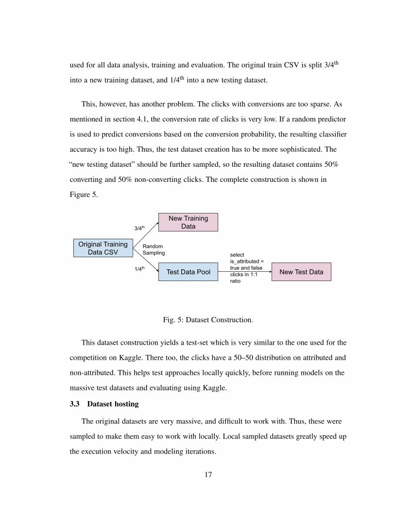
accuracy is too high. Thus, the test dataset creation has to be more sophisticated. The

“new testing dataset” should be further sampled, so the resulting dataset contains 50%

converting and 50% non-converting clicks. The complete construction is shown in

Figure 5.

Original Training Data CSV

New Training Data

Test Data Pool New Test Data

3/4th

1/4th

select is_attributed = true and false clicks in 1:1 ratio

Random Sampling

Fig. 5: Dataset Construction.

This dataset construction yields a test-set which is very similar to the one used for the

competition on Kaggle. There too, the clicks have a 50–50 distribution on attributed and

non-attributed. This helps test approaches locally quickly, before running models on the

massive test datasets and evaluating using Kaggle.

3.3 Dataset hosting

The original datasets are very massive, and difficult to work with. Thus, these were

sampled to make them easy to work with locally. Local sampled datasets greatly speed up

the execution velocity and modeling iterations.

17

At the same time, certain nuances can only be captured by looking at the entire data.

For instance, in section 7.2.3, the heuristic uses the notion of a session. Session-based

rules can only be effective if sessions can be accurately identified in their entirety.

Sampling, however, prevents that from happening, and yields much smaller sessions. In

such cases, some jobs were run in a cloud environment, to allow pulling data based on

database queries close to the source of data.

The datasets were thus, additionally, hosted in a Google Cloud Platform project, using

BigQuery. BigQuery is a big-data analysis solution available on Google Cloud Platform.

It allows automatically parsing the CSV datafiles from the original TalkingData datasets,

and creating tables. The tables can be queried using a GUI interface provided by the

BigQuery UI, enabling running analysis quickly. It also provides SQL-like query interface

on the data, to perform complex queries.

The BigQuery interface is also useful for splitting the data into component sub-tables.

As described in section 3.2, it is important to split the original training dataset into the

real test and training datasets used by the project. Through BigQuery, it is very easy to

perform the splits. For instance, if we wanted to split a table tablename into two tables,

one with 3/4th and the other with 1/4th of data randomly:

SELECT *FROM ‘ad_fraud.Fraud.orig_train_dataset‘ WHEREMOD(FARM_FINGERPRINT(CAST(click_time AS STRING)), 4)in (0, 1, 2) -> new_train_dataset

SELECT *FROM ‘ad_fraud.Fraud.orig_train_dataset‘ WHEREMOD(FARM_FINGERPRINT(CAST(click_time AS STRING)), 4) = 3-> new_test_dataset

18

Similarly, for creating the final test set with 1:1 attributed and unattributed clicks, a

query similar to the following could be done:

SELECT *FROM ‘Fraud.new_test_dataset‘WHERE is_attributed = 1

UNION ALL

SELECT *FROM ‘Fraud.new_test_dataset‘WHERE is_attributed = 0 and RAND() < 0.00247-> final_test_dataset

19

4 EXPLORATORY DATA ANALYSIS

In this section, we describe the exploratory data analysis (EDA) carried out on the

TalkingData dataset [16].

4.1 Conversion Sparsity

Conversions are very sparse in the TalkingData datasets [16]. In fact, only 0.2479% of

ad clicks in the training dataset have attributed conversions. Thus, even a random

predictor, using 0.2479% as the prediction probability for conversion, shows high

precision. On the test dataset, this predictor had an accuracy of 98.1805%. Similarly, on

such a dataset, a predictor which always predicts a click as “not converted” would achieve

an over 99% precision. This is why the test dataset has to be crafted more carefully. The

actual test dataset will include a significant percentage of clicks which were attributed.

This would help in measuring the deltas between models much better and provide a better

prediction accuracy baseline.

As mentioned in section 3.2, finally a test dataset consisting of 1:1 attributed and

unattributed ad clicks is used. On running the aforementioned random predictor on this

dataset, the accuracy is 49.49%. In fact, if the predictor always predicted “fraud” or “not

fraud”, the theoretical accuracy would be 50%. This accuracy should be considered

baseline for all the models. Each legitimate model is expected to have a better than a 50%

prediction accuracy.

Note that this has a side-effect of understating the precision. In real-world traffic, one

would not expect to see conversions on most clicks. In this case, however, the converting

clicks have been amplified. Additionally, in the real-world traffic, it is easier to identify

the non-converting clicks. Thus, a 90% precision on the modified test set might actually

translate to a much higher precision on a real-world traffic dataset. As such, the precision

numbers stated in the experiments to follow should be treated as under-estimates.

20

4.2 Clicky IPs

In the dataset, ‘clicky’ IPs are quite common. There are many IPs with a large number

of clicks. At the same time, many of these IPs with a large number of clicks have abysmal

conversion rates (see Table 3).

Table 3: Clicky IP Addresses (with #clicks≥ 100) vs. Non-Clicky IPs

Clicky Non-Clicky IPs# Clicks 90196132 2283967

# Conversions 117040 112208Conversion Rates 0.13% 4.91%

As is evident from the data, there is a substantial difference in conversion rates

between clicky and non-clicky IPs. Non-clicky IPs have a conversion rate close to 5%,

which is quite practical [17]. Clicky-ness is a major indicator of conversion rates.

Therefore, clicky-ness should be considered as an important feature in model training.

Heuristic models can rely on this to identify IPs which are more likely to convert.

At the same time, the clicky IPs contribute more than 50% of conversions, hence can’t

be all considered fully spammy. This is partly because at least some of these clicky IPs

represent scenarios where a single IP spans across a large number of users. For instance,

the IP could be that of a router in a workspace with many dozens of users. In such

scenarios, it is completely possible to have a large number of clicks and a substantial

volume of conversions. The challenge is in being able to separate out these two kinds of

IPs.

4.3 Relationship between #Clicks and Conversion Rates

While highly clicky users convert at a far lower rate, in general there is also a

relationship between number of clicks and the observed conversion rate. For legitimate

21

users, it is expected that the conversion rate would go down as the number of clicks

increase. For instance, a user might click on an app download ad multiple times, but

might ultimately download the app only once. Figure 6 shows the average conversion

rates observed in the training data set for IPs with the corresponding number of clicks.

Note that there are many users (IPs) which only have a single click, but have a very high

(96%) probability of a conversion. This is again something a heuristic model could utilize

in its rules. Similarly, this points to the number of clicks being a significant estimator of

conversion rates for other kinds of models as well.

Fig. 6: IPs’ Conversion Rates by Number of Clicks.

4.4 Apps and Conversion Rates

There are 700+ app ids in the dataset, numbered starting from 1. Apps conversion

rates across these ids vary very significantly. Figure 7 shows a visual representation of

conversion rates by app ids. There are certain apps which have a nearly 100% conversion

rate, whereas certain other apps which have a close to 0% conversion rate. This indicates

that app is an important feature. For rate-based models, app_cvr can also be used as a

22

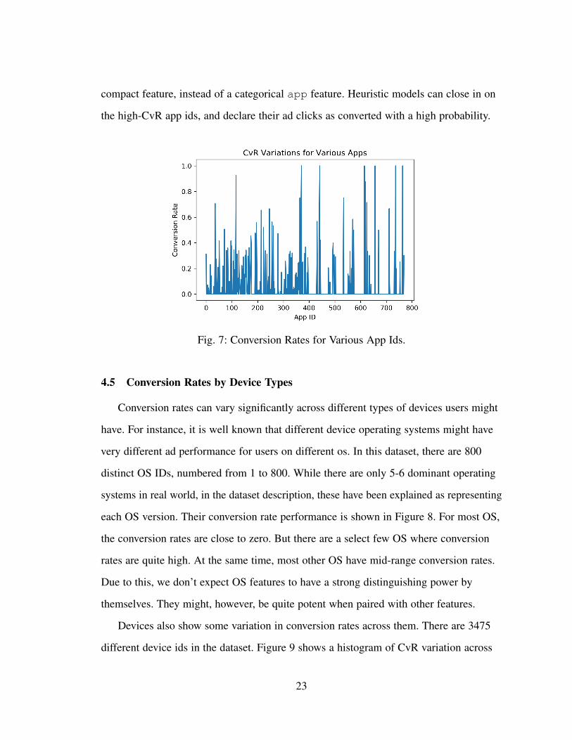
compact feature, instead of a categorical app feature. Heuristic models can close in on

the high-CvR app ids, and declare their ad clicks as converted with a high probability.

Fig. 7: Conversion Rates for Various App Ids.

4.5 Conversion Rates by Device Types

Conversion rates can vary significantly across different types of devices users might

have. For instance, it is well known that different device operating systems might have

very different ad performance for users on different os. In this dataset, there are 800

distinct OS IDs, numbered from 1 to 800. While there are only 5-6 dominant operating

systems in real world, in the dataset description, these have been explained as representing

each OS version. Their conversion rate performance is shown in Figure 8. For most OS,

the conversion rates are close to zero. But there are a select few OS where conversion

rates are quite high. At the same time, most other OS have mid-range conversion rates.

Due to this, we don’t expect OS features to have a strong distinguishing power by

themselves. They might, however, be quite potent when paired with other features.

Devices also show some variation in conversion rates across them. There are 3475

different device ids in the dataset. Figure 9 shows a histogram of CvR variation across

23

Fig. 8: Conversion Rates for Various OS Ids.

these devices. Here again, the differences in conversion rates is lower, with most

conversion rates well away from 1.0. Therefore, it is expected that device features, by

themselves, won’t have a high distinguishing power, unless they are paired with other

features.

Fig. 9: Histogram of Conversion Rates Across Various Devices (with clicks≥ 100)

24

4.6 Channel Conversion Rates

On the channel dimension, the conversion rates do not show significant variation.

Figure 10 shows the range of conversion rates observed across channels. On the y-axis, %

of total conversions covered by channels falling in those conversion rate buckets is

presented. This shows that most of the conversions come from channels with very low

conversion rates. There are, however, a small number of channels with significant

conversion rates. As such, the expected utility of channel ids to identify convertible clicks

is low. Yet, it can not be fully ignored either, due to the presence of a few channel ids

with significant conversion rates. Semantically, channels are very important to ad fraud

detection. Channels represent publishers, and publishers have a strong revenue-incentive

to fake ad clicks.

Fig. 10: % of Conversions in Channels Against the Channel CvRs

4.7 Conversion Rate Time Series

Conversion rates vary significantly across the hour of day. Figure 11 shows a

timeseries of hourly conversion rates, superimposed with click volumes. Conversion rates

in peak hours are nearly double of conversion rates in non-peak hours. The peaks of

25

conversion rates and clicks coincide. Interestingly, there are a few hours with fewer clicks

but relatively higher conversion rates as well. This indicates that conversion rate by hours,

or the hour of day, should be an important feature used for fraud detection.

Fig. 11: Conversion Rate Time Series

26

5 SYSTEM DESIGN

This section describes the system used to perform model training and evaluation. The

system developed provides a seamless way to train and test multiple models and their

variants, and is capable of running well locally as well as on a cloud platform. The overall

system design is provided in Figure 12.

Fig. 12: System Design

At the core, the system has two DatasetProcessors. These processors work to

process specific datasets, for a specified job. Two different implementations of the dataset

processors: ModelTrainer and ModelEvaluator provide the mechanisms to train

and evaluate the models respectively. These data processors rely on a dataset layer to pull

27

the data from appropriate sources. These sources could be either the local datasets, or

tables hosted on BigQuery. The latter is useful when running the processors in a cloud

environment. The dataset layer is capable of performing random sampling of the input

data at the specified rates.

The data processors load model and variant configurations from JSON files. These

files provide information about model tuning parameters to use, as well as the features to

add, drop and transform. A common scheme of specifying (model, variant) has been

used, to have an easy way of referencing the various model settings combinations. Based

on the features, the data processors at times might load ‘Side Tables’. These are

pre-computed pieces of data side-loaded by the data processors to speed up calculations.

For instance, for CvR-space models, all the dimensional CvRs are side-loaded and joined

with the datasets. These ‘Side Tables’ are generated by various Jupyter notebooks offline.

Finally, the data processors also access and modify models in a persistence layer.

Model persistence is important as it allows training a model once while allowing testing it

multiple times on different datasets. Notably, a model trained in a cloud environment can

be tested locally on a smaller test dataset, and vice-versa. Two persistence mechanisms

were used: Google Cloud Storage and local files. These can be used interchangeably

across both the cloud and local environments, to allow rapid experimentation.

28

6 MULTI-LEVEL PERCEPTRONS

As the first step in research work, a multi-level perceptron network was attempted for

the classification problem. This was to establish a baseline for precision, accuracy and

performance against which other, more simplified methods could be compared. Machine

learning models, based on MLPs and Neural Networks, are being increasingly used in the

industry for classification problems, including ad fraud detection. Multi-level perceptrons,

also popularly known as neural networks, have gained a lot of prominence in

classification tasks over the last decade. As such, they serve the purpose of establishing a

baseline performance on the given dataset at hand.

A perceptron models a single neuron, and is combined together to form larger neural

networks. Mathematically, neural networks are able to learn a mapping function from

inputs to output, and have been proven to be a very good universal approximation

method [18]. Their predictive capability originates from their multi-layered structure.

With this structure, they are capable of learning and representing features at various

different scales. Multiple variants of the MLPs were attempted in various configurations,

in order to get reasonable performance and accuracy.

6.1 MLP Construction

For the best performing model, the feature space used for MLPs was based on one-hot

encoding of all categorical fields in data (device, os, channel, app). Additionally, the

click-time was expressed into two features: click day and click hour. IP addresses were

dropped from the data altogether. The MLP, thus, had 1379 input features in the training

dataset. Two hidden layers were constructed, one with 48 perceptrons and the other with

24. Both these layers were set to have a hyperbolic tangent (tanh) as the activation

function. Finally, since a binary classification is desired, an output layer consisting of one

perceptron was constructed, with a sigmoid activation function. The Adam optimizer [19]

29

was used to minimize the binary cross-entropy loss [20]. In terms of training data, the

classifier was trained with about 1% of available training set, using random sampling. To

perform the training, 3 rounds were performed (2 rounds had a large loss, more than 3

rounds didn’t yield much better results incrementally).

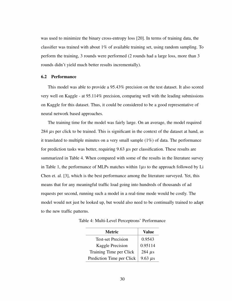
6.2 Performance

This model was able to provide a 95.43% precision on the test dataset. It also scored

very well on Kaggle - at 95.114% precision, comparing well with the leading submissions

on Kaggle for this dataset. Thus, it could be considered to be a good representative of

neural network based approaches.

The training time for the model was fairly large. On an average, the model required

284 µs per click to be trained. This is significant in the context of the dataset at hand, as

it translated to multiple minutes on a very small sample (1%) of data. The performance

for prediction tasks was better, requiring 9.63 µs per classification. These results are

summarized in Table 4. When compared with some of the results in the literature survey

in Table 1, the performance of MLPs matches within 1µs to the approach followed by Li

Chen et. al. [3], which is the best performance among the literature surveyed. Yet, this

means that for any meaningful traffic load going into hundreds of thousands of ad

requests per second, running such a model in a real-time mode would be costly. The

model would not just be looked up, but would also need to be continually trained to adapt

to the new traffic patterns.

Table 4: Multi-Level Perceptrons’ Performance

Metric ValueTest-set Precision 0.9543Kaggle Precision 0.95114

Training Time per Click 284 µsPrediction Time per Click 9.63 µs

30

These results are referred to as a baseline for other methods explored. From here on,

the emphasis is on exploring simplified classification models, with the aim to get a better

trade-off between precision and training/prediction time.

31

7 HEURISTICS

The first few attempts at simplifying the classification task to achieve better

performance were based on heuristics. Heuristic models are an age-old way of performing

classification tasks. These models mimic natural methods of classification. These methods

might be mildly or significantly imperfect, but the hope is that they provide a solid

classification scheme when various heuristic rules are grouped together. Heuristic models

tend to be nearly fully explainable – it is easy to understand why a certain label was

predicted vs. not. They require little to no training. Execution-wise, heuristics just apply

the rules to incoming data, and tend to be extremely fast.

Heuristic models rely on a number of rules executed on the dataset. As an example, a

rule can say: predict a click as converted if num ip clicks = 1. These rules are learnt by

understanding the problem space, as well as data characteristics, very deeply. As such,

they tend to be highly domain-dependent, as well as highly data-dependent. This is quite

different from most machine learning models, where the models themselves follow a

uniform framework, and feature engineering is the real work. Despite machine learning

gaining prominence in the last decade, heuristic models are still very popular. Their

explain-ability and deep knowledge of data are a major asset.

7.1 Sessionization

Some of the heuristics explored use the concept of ‘sessions’. A session can be

defined as contiguous click activity (potentially spanning multiple ad clicks across

multiple apps and channels) originating from a single IP address. Additionally, a session

must be constrained to emanate from a given set of (os,device). OS and Device could act

as a proxy for identifying a single user within an IP address used by multiple users. While

not perfect (ideally, one would use a Cookie Id or a logged-in User Id), it significantly

increases the number of single-user activity sessions available to analyze. Various

32

session-level metrics can be defined and used as features for heuristics as well as even in

machine learning models.

7.2 Heuristics Explored

In this section, various heuristics for the problem at hand are described. Note that

these heuristics may not generally apply to any ad click dataset for conversion or

fraud-click detection. Instead, these are very specific to the problem+datasets at hand.

Nevertheless, these heuristics have the potential to demonstrate strong wins in prediction

accuracy. The remainder of this section discusses the various heuristics explored and used.

7.2.1 High attribute conversion rate

The dataset at hand has a generally low conversion rate. The probability of any

random ad click being attributable is lower than 1%. At the same time, there are a few

signals which show strong conversion potential. For instance, if it is known that a given

IP address only has one click, the data analysis (Figure 6) shows that it is over 98% likely

for this click to get attributed. This heuristic exploits this fact. It looks at all the attribute

values for a given ad click, to see if there is any attribute which has a fairly high observed

conversion rate on training data. If so, it declares the click has converted. Note that this is

only workable because the typical conversion probability if a random click is very, very

low. If, on the other hand, it was meaningfully high (even, say, 10–20%), this heuristic

would incur significant error rate. Additionally, this heuristic also provides a fairly high

rate of false positives too. Yet, the overall precision of this heuristic was 98%, which is

very high.

7.2.2 IP's clicks too high in an hour

This is a negative heuristic. On finding IPs which have significant bursts of traffic in a

given hour, these IPs'clicks can be marked as non-converted for that hour. This could be

despite the fact that other rules predict a positive conversion outcome.

33

7.2.3 Session's last click is convertible

A user might legitimately perform multiple ad clicks in a given session. This could be

because the user might be researching and exploring whether the app meets their needs

and has the appropriate features. In this process, they might perform various searches,

interact with ads at various times, before they ultimately download the app. If it was

known that an IP address belongs to a single user (or a single household), the prior ad

clicks can be discounted for conversions, and instead the conversion can be attributed to

the last click in the session. This heuristic requires understanding and segmenting the user

sessions.

7.3 Heuristic Combination

Different heuristics might provide conflicting positive and negative signals for a few

clicks. That makes it difficult to provide a single answer for a click. Additionally, some

signals might carry more weight than others – so a positive signal from one heuristic

might be overridable by a negative signal from another heuristic with a higher weight. To

capture these nuances, a heuristic combination method was built. Each heuristic specifies

the predictive positive signal, based on its conviction. These predictive signals are then

merged and clipped to arrive at the final answer. This provides a flexible framework to

express and work with a large number of potential heuristics. The combination method is

described in Algorithm 1.

7.4 Heuristic Results

The various heuristics’ precision and recall is provided in Table 5. Coverage or recall

here is defined by the % of converting clicks which the rule can identify (and, notably, not

on the base of all clicks).

On their own, the heuristics did not yield very favorable results. This is because

heuristics in this dataset have a high bar on their precision to be useful for classification.

34

Algorithm 1 Heuristic Combination Algorithm

1: procedure COMPUTEANDCOMBINEHEURISTICS(Data, Heuristics, Weights)2: Results← /03: for each d ∈ Data do4: credits← 05: for each h ∈ Heuristics do6: score← h(d)7: credits← credits+Weightsh ∗ score8: if credits≤ 0 then9: prediction← 0

10: if credits≥ 1 then11: prediction← 112: Results← Results+[prediction]13: return Results

Table 5: Heuristics’ Performance

Heuristic Precision CoverageHigh Conversion Rate Attributes 0.98 0.1737Single-click Sessions Convertible 0.1467 0.1998

Last Click Convertible 0.3853 0.112

The model effectiveness depends on the rules’ precision. If the dataset has a low natural

positives rate, it would typically require rules with more than 50% precision for the rules

to be effective. The relationship is described in the equation below.

Pr(positiveLabel)+Precisionheuristic > 0.5 (1)

where: Pr(positiveLabel) = Probability a random observation has a positive label, and

Precisionheuristic = Precision of positive predictions by the heuristic. In the dataset,

Pr(positiveLabel) is 0.25%, which is really low. Because of this, only those heuristics

help which have more than a 50% precision. Only one such heuristic was found: the high

conversion rate heuristic described in section 7.2.1. A few other heuristics were identified,

which, while would be typically quite effective, were stymied by the low random

35

observation positive probability. Some very high-precision heuristics are possible to

identify, but they suffer from coverage problems.

There are many negative heuristics available as well, such as bursty-IPs, etc. Given the

dataset, however, these are not very effective. Due to a low Pr(positiveLabel), most

clicks are anyway likely to be negatively identified as non-converting. As such, the

negative heuristics do not add much value. For instance, while the ‘Clicky-IP’ heuristic

clearly identifies a much higher average conversion rate in non-high-click IPs, it leaves

out 50% of conversions which are done by high click IPs.

At the same time, heuristics do yield interesting insights into simplistic features and

classifiers which can yield good results. Heuristics here have demonstrated a much higher

precision than what’s expected of a random observation probability, which means they

carry a positive signal. Yet, it is evident that they might not ultimately lead to good

models. A model trained with these heuristics put together could only surmise a 62%

precision on the test dataset. This result compares closely with multi-model evidence

fusion work done by Mehmed et. al [6], who also used multiple weak sensors and

combined data across them, and obtained a 64% precision. Yet, 62% is a weak precision

for a classifier, and leads to a noisy output. The expectation is to be able to classify most

of the clicks correctly, and heuristics fell short of doing that.

36

8 MACHINE LEARNING MODELS

After the heuristics, a few machine learning models were attempted. The idea was to

keep a small feature set, and get models with reasonable accuracy (close to 90%

precision) and good performance suitable for real-time applications (one order of

magnitude improvement over MLPs). This section describes the various machine learning

models attempted, along with their various variants, configuration settings and features.

8.1 Features

Even though the original dataset is limited in the number of features provided, a

variety of features can be extrapolated from the given dataset. These features have the

potential to add more distinguishing power in the models. A comprehensive list of

features used in machine-learning models across the various trials is provided in Table 6.

A subset of these features was chosen for various different types / variants of these

models. In the next few sub sections, details on various different types of models and

variants are provided.

8.1.1 Feature Descriptions

Many of the features described above are self-explanatory, though some aren’t. These

other features are briefly described below.

click day and hour of day: These have their typical meanings. One important point

to note is that these have been used in both categorical and non-categorical fashion in

different model variants.

ip num clicks: Number of clicks observed from the given IP. To cover the entire

timeline spectrum, these counts have been done on both the training and test data put

together. As seen in EDA Section 4.3, number of clicks observed for an IP is an important

signal to consider.

37

Table 6: Machine Learning Model Features

Feature Descriptionapp App Id of the Ad Click

device Device Id of the Ad Clickos OS Id of the Ad Click

channel Channel Id of the Ad Clickhour of day Click's Hour of Day

click day Click's Dayip num clicks IP's #Clicks in Train+Test Periodone click ip If the IP only has 1 Ad Click

ip num click cvr Avg CvR of IPs having this IP's #Clicksapp cvr Avg CvR of Ad Click's App Idos cvr Avg CvR of Ad Click's OS Id

device cvr Avg CvR of Ad Click's Device Idchannel cvr Avg CvR of Ad Click's Channel Id

hour cvr Avg CvR of all clicks in Ad Click's Hourip day hour click count Count of clicks grouped by ip-day-hour

ip app click count Count of clicks from an IP for an App Idip app os click count Count of clicks from an IP on an OS for an App Id

ip app channel variance click day Variance in click days for an (IP, App, Channel)

one click ip: Related to above, is a boolean feature. The signal provided by

ip num clicks dissipates rapidly after 1 click. This feature helps capture this particular

aspect.

ip day hour click count: Helps look at the IP’s burstiness in a given hour.

Bustry-ips in a given hour are less likely to lead to conversions.

ip app click count: Attempts to capture spam perpetrated by ‘competitors’, by

helping identify IPs which fire a lot of clicks for a given app.

ip app os click count: Goes one level deeper on the above signal. Some IPs are

multi-user IPs, and this one helps identify specific devices or users the fraud ad clicks

might be coming from.

38

ip app channel variance click day: Attempts to identify if most clicks from an IP

for an App on a Channel occur within a short timeframe. The overall idea is that, if this

variance is high, the user is performing lots of clicks on a regular basis, without any intent

to download the app.

8.2 Base Models

As the most simple modeling method, the raw signals in the data were directly used as

features for various types of ML models. These models have been referred to as “base

models” in this thesis. IP addresses were dropped, but other dimensions were used as

non-categorical features. Click time was dropped but replaced by hour of day. This way,

the set of features was kept very small - only 6 features used for training and

classification.

Multiple types of ML models were used. From literature survey, gradient boosting

model, Linear-SVC and K-NN stand out. Additionally, Naive-Bayes was also explored,

being a very simple modeling technique. All these different ML models were trained

using various random samples of training data. The reason behind varying the training

sample sizes was to optimize for precision while minimizing over-fitting.

Table 7: Base Models’ Performance

Model Sample Precision Trn. cost (µs) Pred. cost (µs)Linear-SVC 0.001 0.5003 5.9643 0.0595Linear-SVC 0.01 0.5000 8.1099 0.0475

Naive-Bayes 0.01 0.5469 0.1908 0.1364Naive-Bayes 0.001 0.5445 0.2131 0.1363

k-NN 0.001 0.5000 2.2873 30.9784

G-Boost 0.001 0.7105 14.8722 0.3632G-Boost 0.01 0.5933 22.9355 0.3520

The results for base models are summarized in Table 7. Even with such simplistic

features, some good insights can be drawn. LinearSVC and k-NN performed poorly,

39

achieving 50% precision. In fact, looking at their outputs, they nearly always predicted

zeroes (except for 1-2 clicks in both cases): which means that those clicks did not convert.

This is because of the way these two models work, and the nature of features provided to

them. k-NN, for instance, relies on looking at the ’k’ nearest neighbors in the feature

space for a given click being predicted. The distance used here was L2 distance, with a

k = 5. A L2 distance would mean that device=10 and device=11 are devices with close

similarity, compared to device=10 and device=100. This clearly isn’t true in this dataset,

however. Features like device are categorical. So, L2 distance is meaningless in this space.

LinearSVC also relies on a similar mechanic. Even Naive-bayes’s classification is weak

due to this reason, though it achieves a slightly better precision at 54.69%.

On the other hand, gradient-boosting performance was the best among the models

attempted. With a 0.1% training data sample, a 71% precision is obtained. This is despite

the fact that the features have been treated as continuous and not categorical. This is

because gradient boosting does not rely on a notion of L2 distance, and is instead

attempting to perform gradient descent from labels to learn which labels are likely to

yield positive outcomes. Gradient boosting model’s performance, however, went down

significantly when 10X training data was provided. This is suggestive of over-fitting. The

base gradient boosting model with 71% precision classifies better than the heuristics (refer

back to Table 5). The model’s prediction time is only 0.32 µs per click. When compared

to MLP model’s prediction time of 9.63 µs per click, this is an order of magnitude lower.

Yet, the precision is not as high as we had set out to look for.

8.3 One-hot Encoded Feature Space

In Section 8.2, LinearSVC and k-NN performed poorly because the feature space was

not conducive for distance calculations. This is typically avoided by transforming

categorical features into a one-hot encoding. In one-hot encoding, each feature-value

becomes a distinct feature. For instance, if the device feature can take values from 1 to

40

100, it would be transformed into 100 features, representing

device1,device2, . . . ,device100. Now, for each click, only one of these 100 features would

have a value of 1 or true, while all others would have zeroes. In such a space, distance

functions begin to become more useful. Now a click from device=1 is similarly distant

from a click from device=10 versus another click from device=100, assuming all other

dimensions are identical.

One-hot encoding variants were created for each type of model. All categorical

features: os, device, app and channel were transformed to be one hot encoded. As in

Section 8.2, IP addresses were excluded and click time was replaced by hour of day. In

addition, ip num clicks was also included, to represent distance on IP addresses based on

a very identifying feature such as number of clicks (see Section 4.3). In total, this

transformed the feature-space into 5589 dimensions. The results are summarized in

Table 8.

Table 8: One-hot Models’ Performance

Model Sample Precision Trn. cost (µs) Pred. cost (µs)Linear-SVC 0.001 0.6304 108.4241 70.7381Linear-SVC 0.01 0.6330 211.9565 76.1893

Naive-Bayes 0.001 0.6964 126.7783 114.2180Naive-Bayes 0.01 0.6140 296.6669 104.8078

k-NN 0.0001 0.0860 500.8176 11509.5484

G-Boost 0.001 0.5010 17.3676 63.5168G-Boost 0.01 0.6535 31.5229 66.1342G-Boost 0.02 0.5417 39.7130 64.7975

Naive-Bayes is the best model in this feature space. It benefits from meaningful

L2-distances. With a training sample of 0.1%, sufficient learning is achieved and it

provides a nearly 70% prediction precision. While LinearSVC improves as well when

compared to the base feature space, the improvement is not as much as for NaiveBayes.

41

This is because the surface separating the converted and non-converted clicks in this

hyperspace might not be express-able as a plane. NaiveBayes can handle this scenario

better, compared to LinearSVC.

k-NN, on the other hand, deteriorates and becomes much worse. This is, however,

attributable to k-NN’s smaller training sample. k-NN models are very bulky, as they need

to store each data point in a high-dimensional space. These models were trained here in a

5589-dimensional space. This required us to reduce the training sample massively, but it

significantly ended up affecting the precision. Even with such a small sample, k-NN

models took 11.5 ms to lookup for each click, which is extremely costly. Sampling was

needed even while performing evaluations (unlike any other ML model tried in any

feature-space). It can be concluded that one-hot feature space is not conducive to k-NN.

Gradient-boosting shows interesting trends. Working in a much bigger feature-space,

the precision drops sharply for the 0.1% training sample. This indicates that the decision

trees find it difficult to classify clicks when the feature space is very large. As expected,

however, the precision improves when this model is provided more data. More input is

required to have the decision trees converge across a larger feature-space. Beyond a point,

however, over-fitting becomes a concern again.

Across all the models in one-hot encoding feature space, the performance trends are

very clear. There is a significant cost paid for working in a high-dimensional feature space

such as this. When compared to performance on base features as shown in Table 7, the

prediction and training costs have all gone up by over 100X. Clearly, while most models

improve in precision in this space, their utility for real-time classification of ad fraud is

limited due to their cost.

A common issue with one-hot feature spaces is about relative weights. When features

are one-hot encoded, one has to reason about distance between features from the same

raw feature (eg. L2(device1,device5)) versus distance between features across different

42

raw features (eg. L2(device1,os20)). This creates a challenge for models which use

distance functions, as opposed to loss functions, such as NaiveBayes and LinearSVC. On

the other hand, such a space is very conducive for classifiers meant for categorical spaces,

and even neural networks tend to work better with such spaces. In fact, the MLPs

evaluated in Section 6 also use one-hot encoded features, and provide a 95% precision.

8.4 CvR Space

So far, NaiveBayes and LinearSVC models have demonstrated better cost

performance when working with a small number of features. If one could create a feature

space with small number of features which these models could exploit better, there is a

good chance that a better precision could be achieved at a small computation cost. This is

the motivation behind exploring the CvR space.

The original dataset predominantly consists of categorical features. If these categorical

features are used as is, this leads to lower precision (see ‘base’ variants’ performance in

Table 7). This is because most models assume a continuous feature axis per feature. Thus,

ip = 100 and ip = 101 are treated as almost identical, even though these really don't have

much in common, apart from a happenstance of their values being close.

One way to deal with categorical features without blowing up the feature space is to

use conditional probability coding [21]. The basic idea of conditional probability (CP)

coding is to replace each categorical feature with its conditional probability of predicting

the label value. Since the training labels for ad fraud detection are binary (0 =

non-converting click, 1 = converting click), CP-coding is possible. Each categorical

variable (os, device, channel) is replaced by their CP-coding. eg. os = 10 is replaced by

Pr(is attributed = 1 | os = 10). Additionally, the method is applicable to non-categorical

variables too. For instance, it could be applied to ‘hour of day’ as well, by replacing it

with the probability of conversion in a given ‘hour of day’. The result of these transforms

is a “CvR Space”. This is a n-dimensional space, where each axis represents the

43

conditional conversion rate (CvR) of a particular feature. The expectation is that

converting and non-converting clicks can be separated out in this space easily. For

instance, converting clicks will gather closer to the point (1,1, . . . ,1), whereas the

non-converting clicks will gather closer to (0,0, . . . ,0). Results for various model trials

with CvR space are listed in Table 9.

Table 9: Models’ Performance in Conversion-Rate Space

Model Sample Precision Trn. cost (µs) Pred. cost (µs)Linear-SVC 0.001 0.6258 0.7550 0.0599Linear-SVC 0.01 0.6440 0.8243 0.0519Linear-SVC 0.05 0.6477 0.8678 0.0546

Naive-Bayes 0.001 0.8996 0.1599 0.1365Naive-Bayes 0.01 0.8997 0.1624 0.1354

k-NN 0.001 0.6093 7.6525 54.2434k-NN 0.01 0.6868 108.3013 294.7478

G-Boost 0.001 0.6909 8.4141 0.4233G-Boost (1pc) 0.01 0.6816 9.7152 0.4092

CvR-space shows good improvement in Naive-Bayes model’s precision, going up to

90%. Naive-Bayes also shows good performance from a cost perspective, requiring only

about 0.26 µs to train per click, and 0.136 µs to lookup for each click. The model was

also used to predict the labels for the Kaggle test dataset. Kaggle score was quite high too,

at 89.33% precision. The model precision and training/prediction costs fit within the

real-time classifier parameters laid out earlier.

In addition, CvR space provides improvements for other models too. LinearSVC

exhibits similar precision as the one-hot encoding feature space (64.77% here vs 63.30%

in on-hot encoding space), but with significantly reduced prediction cost (0.0546 µ s here

vs 76 µ s for one-hot encoding). The precision performance is attributable to a similar

concern on CvR-space not being separable by a plane to classify converting and

non-converting clicks well. Gradient-boosting also keeps its 69% precision, but at a

44

reduced training cost when compared to the base variant. Gradient-boosting model

required to be tuned differently for the different training sample sizes, to get optimal

precision.

Finally, k-NN shows improvements in classification accuracy, particularly when

working with a larger sample size, taking precision to 68.68%. This is because, in this

space, the distance functions are the most meaningful. Distances are now normalized

across feature-dimensions, leading to better distance measurement. A big caveat with

k-NN, however, is its cost. As can be seen, when the training sample size grew by 10X,

there were significant increases in training and prediction costs as well. Training cost

grew by more than 10X. The model size was large as well, making it impractical to train

the model over even bigger samples, without utilizing a large number of machines.

8.5 IP Aggregate Features

So far, IP addresses have not been used in the models. The number of distinct IPs are

over 100K, and there are IP addresses in test sets (both the synthetic test set, as well as

the Kaggle private test set) which are not present in training dataset. Additionally, IP

addresses have not been provided in their usual 32-bit format with their subnets, etc. IPs

are basically categorical in this dataset, and no information could be derived by just

looking at the IP addresses (presumably, for privacy reasons). This limits their utility, as

some potentially useful features such as subnets, geo-location, etc cannot be obtained.

There is potential to aggregate various kinds of information on IP-addresses, however.

Similar to the sessionization introduced in Section 7.1, various statistics can be computed

on aggregates where IP is at least one of the dimensions. Many of these features have

been mentioned in Table 6. The machine learning models were trained with these

additional aggregate features, to see if IP addresses could provide useful classification

signal as well. Note that these features were treated as continuous, instead of categorical.

The results have been tabulated in Table 10.

45

Table 10: Models’ Performance with IP Aggregate Features

Model Sample Precision Trn. cost (µs) Pred. cost (µs)Linear-SVC 0.001 0.5425 64.1757 0.0645Linear-SVC 0.01 0.5425 73.3807 0.0813

Naive-Bayes 0.001 0.5749 0.2711 0.2409Naive-Bayes 0.01 0.5744 0.2737 0.2391

k-NN 0.001 0.5860 138.3072 98.1994

G-Boost 0.001 0.5425 6.2003 0.4083G-Boost 0.01 0.5722 15.8315 0.3642

The results show that there is some signal in these ip-aggregate features, but overall

the precision is lower than the other models. This implies these features could provide

minor improvements in precision only.

46

9 RESULTS

In this thesis, multiple experiments were conducted to evaluate the utility-cost

tradeoffs for classification, with the goal of identifying prediction methods suitable for

real-time ad fraud detection. The precision and performance metrics for various methods

have been provided in Table 4 for MLP, Table 5 for heuristics, Table 7 for ML models

with base features, Table 8 for models with one-hot encoded features, Table 9 for models

in CvR space and Table 10 for ML models working with IP-aggregates as features. Note

that, as mentioned in Section 4.1, these precisions are strict lower-bounds of the true

precision, as they have been computed on a skewed test-set, to allow judging the model

performance better.

Based on the experiments, machine learning methods based on neural networks /

multi-layer perceptrons have the best precision at 95.43% among the models attempted.

These models have a prediction time at 9.63 µs per click. The model is costly to train as

well, requiring 284 µs per click, comparing unfavorably against most other models

attempted. Put together, due to the higher training and prediction cost, the model’s utility

for real-time classification is limited. Note that the timing method used accounts only for

the model fitting and model prediction times, and ignores the data preparation overhead.

Given the nature of features used by MLP (one-hot encoded), the data preparation phase

is also compute-intensive, and adds on top of the training and prediction time.

Most of the models and feature-spaces capped out at about 70% precision for

classification times less than 1µs. This level of precision provides only a weak classifier

for ad fraud clicks in real-time. Gradient-boosting, widely quoted in literature, provided

71% precision at best in the experiments, working with the base features. Naive-Bayes,

with the exception of CvR space, provided 69.64% accuracy with the one-hot feature

space. k-NN provided the best accuracy of 68.68% working in the CvR space, though the

model size was large and the classification time was close to 300µs. k-NN performed

47

poorly with large feature spaces: specifically had more than 11ms of prediction time in

one-hot encoding space. Linear-SVC only provided 64.47% at best, with the CvR space.

The best classifier for real-time use, among the experiments, was found to be the

Naive-Bayes classifier in the CvR space, providing 89.97% precision. The classifier also

had smaller training and prediction costs, requiring only 0.16µs and 0.13µs respectively.

The model prediction error is close to 2X of the MLP model, while the prediction cost is

less than 1/70th of the MLP model (see Table 4 for comparison).

These top models were also uploaded to Kaggle to evaluate on independent test

datasets. They had identical performance on Kaggle, matching the precision results

obtained over the test sets within 1%. The Naive-Bayes classifier in CvR space scored at

89.33% on Kaggle. This also shows that the test dataset construction in Section 3.2 is

effective, and mimic’ed the Kaggle independent test dataset well.

Put together, the results show that machine learning models are effective in predicting

clicks likely to have conversions, and can produce more than 90% precision. Conversely,

these models are also able to predict which clicks are highly likely to be fraudulent, with

close to 0 probability of conversion. It has also been demonstrated that it is possible to

build models which have low cost, using less than 1µs per click for training and

prediction, and 90% precision. Such models are suitable for real-time ad click fraud

classification.

48

10 CONCLUSIONS AND FUTURE WORK

Based on the results above, it can be concluded that real-time detection of ad click

fraud is possible, using simple classifiers such as Naive-Bayes. Even on this unbalanced

dataset, it is possible to achieve a 90% precision in identifying convertible clicks, while

keeping compute costs below 1µs per click.

There are some other interesting approaches worth exploring in the future.

Gradient-boosting on top of weaker predictive models could be tried. Gradient boosting

could also be attempted with more session-based signals: such as first click in session, or

last click in session. Some of the heuristics demonstrate reasonable precision, and could

be used to create new features which could then be used in various ML models. Other

datasets could be explored, where the data might be more meaningful: for instance with

real IP addresses. These would open up many more features useful for analysis: such as

the geographical location, sub-networks, etc.

More study should be done to build tiered models. Tier 1 could perform real-time ad

click fraud detection with low cost. Output from tier 1 models could be used to perform

incidence response and investigation. Tier 2 models could be more exhaustive, and run

offline. Tier 2 models could also learn from the outcome of Tier 1 models, and thereby be

able to perform better. Such a system would be able to amalgamate the best properties of

real-time and offline classification systems.

Availability of public and labeled datasets for ad click fraud is limited. This limits the

experimentation and research which could be done. There is, however, a possibility of

creating simulated ad click fraud, and melding it with regular website traffic. This could

help evaluate the efficacy of ad click fraud detection under specific types of ad click fraud

attacks: such as botnets, or human clickers. This could also open up many more

interesting features, such as referrer URLs and HTTP headers, along with user ids such as

Cookies.

49

Ultimately, ad click fraud detection is a moving target. As ad networks and advertisers

catch up with the state-of-the-art in ad click fraud, more and more malignant players keep

inventing new methods to circumvent fraud prevention. Thus, it is imperative to continue

the research in this space and continue to catch up to the ad click fraud.

50

Literature Cited

[1] D. Liu, S. Xu, L. Chen, and C. Wang, “Some observations on online advertising: Anew advertising system,” in 2015 IEEE/ACIS 14th International Conference onComputer and Information Science (ICIS), pp. 387–392, June 2015.

[2] X. Li, Y. Liu, and D. Zeng, “Publisher click fraud in the pay-per-click advertisingmarket: Incentives and consequences,” in Proceedings of 2011 IEEE InternationalConference on Intelligence and Security Informatics, pp. 207–209, July 2011.

[3] X. Jiarui and L. Chen, “Detecting crowdsourcing click fraud in search advertisingbased on clustering analysis,” in 2015 IEEE 12th Intl Conf on Ubiquitous Intelligenceand Computing and 2015 IEEE 12th Intl Conf on Autonomic and Trusted Computingand 2015 IEEE 15th Intl Conf on Scalable Computing and Communications and ItsAssociated Workshops (UIC-ATC-ScalCom), pp. 894–900, 2015.

[4] M. Faou, A. Lemay, D. Decary-Hetu, J. Calvet, F. Labreche, M. Jean, B. Dupont, andJ. M. Fernande, “Follow the traffic: Stopping click fraud by disrupting the valuechain,” in 2016 14th Annual Conference on Privacy, Security and Trust (PST),pp. 464–476, 2016.

[5] B. Kitts, J. Y. Zhang, A. Roux, and R. Mills, “Click fraud detection with botsignatures,” in 2013 IEEE International Conference on Intelligence and SecurityInformatics, pp. 146–150, 2013.

[6] M. Kantardzic, C. Walgampaya, and W. Emara, “Click fraud prevention inpay-per-click model: Learning through multi-model evidence fusion,” in 2010International Conference on Machine and Web Intelligence, pp. 20–27, 2010.

[7] G. Shafer, “A mathematical theory of evidence,” International Journal ofApproximate Reasoning, vol. 79, July 2016.

[8] H. Xu, D. Liu, A. Koehl, H. Wang, and A. Stavrou, “Click fraud detection on theadvertiser side,” in Computer Security - ESORICS 2014, vol. 8713, pp. 419–438,September 2014.

[9] A. Dimitris, M. Paschou, E. Sakkopoulos, E. Sourla, G. Tzimas, A. Tsakalidis, andE. Viennas, “Exposing click-fraud using a burst detection algorithm,” pp. 1111–1116,June 2011.

51

[10] Y. Guo, J. Shi, Z. Cao, C. Kang, G. Xiong, and Z. Li, “Machine learning basedcloudbot detection using multi-layer traffic statistics,” in 2019 IEEE 21stInternational Conference on High Performance Computing and Communications;IEEE 17th International Conference on Smart City; IEEE 5th InternationalConference on Data Science and Systems (HPCC/SmartCity/DSS), pp. 2428–2435,August 2019.

[11] R. Mouawi, M. Awad, A. Chehab, I. H. E. Hajj, and A. Kayssi, “Towards a machinelearning approach for detecting click fraud in mobile advertizing,” in 2018International Conference on Innovations in Information Technology (IIT), pp. 88–92,2018.

[12] L. Song, X. Gong, X. He, R. Zhang, and A. Zhou, “Multi-stage malicious clickdetection on large scale web advertising data,” CEUR Workshop Proceedings,vol. 1018, pp. 67–72, January 2013.

[13] M. S. Iqbal, M. Zulkernine, F. Jaafar, and Y. Gu, “Fcfraud: Fighting click-fraudfrom the user side,” in 2016 IEEE 17th International Symposium on High AssuranceSystems Engineering (HASE), pp. 157–164, 2016.

[14] R. A. Costa, R. J. G. B. de Queiroz, and E. R. Cavalcanti, “A proposal to preventclick-fraud using clickable captchas,” in 2012 IEEE Sixth International Conferenceon Software Security and Reliability Companion, pp. 62–67, 2012.

[15] M. Kantardzic, C. Walgampaya, B. Wenerstrom, O. Lozitskiy, S. Higgins, andD. King, “Improving click fraud detection by real time data fusion,” in 2008 IEEEInternational Symposium on Signal Processing and Information Technology,pp. 69–74, 2008.

[16] TalkingData, “Talkingdata adtracking fraud detection challenge.”https://www.kaggle.com/c/talkingdata-adtracking-fraud-detection/data, 2018.

[17] AppTweak, “Average app conversion rate per category [2020].” https://www.apptweak.com/aso-blog/average-app-conversion-rate-per-category-2019,2020.

[18] G. Lewicki and G. Marino, “Approximation by superpositions of a sigmoidalfunction,” Appl. Math. Lett., vol. 17, pp. 1147–1152, 12 2004.

52

[19] D. Kingma and J. Ba, “Adam: A method for stochastic optimization,” InternationalConference on Learning Representations, 12 2014.

[20] S. Mannor, D. Peleg, and R. Rubinstein, “The cross entropy method forclassification,” in Proceedings of the 22nd International Conference on MachineLearning, ICML ’05, (New York, NY, USA), p. 561–568, Association for ComputingMachinery, 2005.

[21] A. Radianto and AirbnbEng, “Designing machine learning models.” https://medium.com/airbnb-engineering/designing-machine-learning-models-7d0048249e69, July2015.

53