real-time correction by optical tracking with … · 1.5 hypothesis statement ... 2.3 pipeline for...
TRANSCRIPT

Real-Time Correction By Optical Tracking with Integrated
Geometric Distortion Correction for Reducing Motion Artifacts in fMRI
by
David. J. Rotenberg
A thesis submitted in conformity with the requirements for the degree of Masters of Science
Medical Biophysics University of Toronto
© Copyright by David Rotenberg 2012

ii
Real-Time Correction By Optical Tracking with Integrated
Geometric Distortion Correction for Reducing Motion
Artifacts in fMRI
David Rotenberg
Masters of Science
Medical Biophysics
University of Toronto
2012
Abstract
Artifacts caused by head motion are a substantial source of error in fMRI that limits its
use in neuroscience research and clinical settings. Real-time scan-plane correction by optical
tracking has been shown to correct slice misalignment and non-linear spin-history artifacts,
however residual artifacts due to dynamic magnetic field non-uniformity may remain in the data.
A recently developed correction technique, PLACE, can correct for absolute geometric distortion
using the complex image data from two EPI images, with slightly shifted k-space trajectories.
We present a correction approach that integrates PLACE into a real-time scan-plane update
system by optical tracking, applied to a tissue-equivalent phantom undergoing complex motion
and an fMRI finger tapping experiment with overt head motion to induce dynamic field non-
uniformity. Experiments suggest that including volume by volume geometric distortion
correction by PLACE can suppress dynamic geometric distortion artifacts in a phantom and in
vivo and provide more robust activation maps.

iii
Acknowledgments
I would like to express my sincere gratitude to the people whose assistance and support without
which this work would not have been possible. First I would like to thank all of the members of
the Graham lab, both past and present, for their help and experience, particularly Mark Chiew
and Fred Tam. I also thank the members of my supervisory committee, Dr. John Sled and Dr.
Anne Martel, for their constructive criticisms and guidance. I want to give special thanks to my
supervisor Dr Simon Graham for his valuable guidance and advice on so many aspects of this
thesis, for encouragement, and for providing me with such a wonderful opportunity. I transmit a
warm thanks to my family and friends for their constant encouragement and support.

iv
Table of Contents
Acknowledgments .......................................................................................................................... iii
Table of Contents ........................................................................................................................... iv
List of Tables ............................................................................................................................... viii
List of Figures ................................................................................................................................ ix
List of Abbreviations ..................................................................................................................... xi
Chapter 1 Introduction .................................................................................................................... 1
1.1 Functional MRI ................................................................................................................... 2
1.1.1 Role of Functional MRI in Neuroimaging .............................................................. 2
1.1.2 Fundamental MRI Physics ...................................................................................... 2
1.1.3 Geometric Distortion In EPI ................................................................................. 16
1.1.4 Static Geometric Distortion Correction in EPI ..................................................... 16
1.1.5 Signal Contrast Mechanisms in fMRI ................................................................... 19
1.1.6 FMRI Experiment and Post-Processing ................................................................ 20
1.2 Motion Artifacts ................................................................................................................ 23
1.2.1 Head Motion and Related Artifacts in FMRI........................................................ 23
1.2.2 Types of Head Motion .......................................................................................... 24
1.2.3 Head Motion in Different Subject Populations ..................................................... 25
1.2.4 Slice Misalignment Artifact .................................................................................. 26
1.2.5 Spin History Artifact ............................................................................................. 26
1.2.6 Dynamic Geometric Distortion Effects................................................................. 27
1.3 Motion Correction Strategies ............................................................................................ 27
1.3.1 Head Restraints ..................................................................................................... 28
1.3.2 Fast Imaging .......................................................................................................... 28

v
1.3.3 Post-Processing Methods ...................................................................................... 29
1.3.4 Spin History Artifact Correction ........................................................................... 30
1.3.5 Real-Time Correction ........................................................................................... 31
1.3.6 Real-Time Scan-Plane Adjustment and Geometric Distortion Correction: An
Integrated Approach .............................................................................................. 33
1.4 Summary of Motivation .................................................................................................... 35
1.5 Hypothesis Statement ........................................................................................................ 36
Chapter 2 Real-Time Correction By Optical Tracking for fMRI with Integrated Geometric
Distortion Correction for Reducing Artifacts in fMRI ............................................................ 37
2.1 Introduction ....................................................................................................................... 37
2.2 Methods ............................................................................................................................. 40
2.2.1 Tracking System Apparatus and Initial Calibration .............................................. 40
2.2.2 Validation of the Tracking System ....................................................................... 42
2.2.3 Coordinate Transformation ................................................................................... 43
2.2.4 Evaluation of Calibration Accuracy ...................................................................... 46
2.2.5 Real-Time Correction System ............................................................................... 47
2.2.6 PLACE Geometric Distortion Correction ............................................................. 48
2.2.7 Evaluation of PLACE ........................................................................................... 50
2.2.8 Imaging Protocols ................................................................................................. 51
2.2.9 Phantom Design .................................................................................................... 51
2.2.10 Phantom Imaging Experiments ............................................................................. 53
2.2.11 In Vivo Experiments .............................................................................................. 56
2.3 Results ............................................................................................................................... 57
2.3.1 Validation of the Tracking System ....................................................................... 57
2.3.2 Tracking System Stability Results ........................................................................ 59
2.3.3 Accuracy of Coordinate Transformation .............................................................. 59
2.3.4 Real-Time Tracking .............................................................................................. 60

vi
2.3.5 Evaluation of PLACE ........................................................................................... 61
2.3.6 Phantom Experiments ........................................................................................... 63
2.3.7 Bilateral Finger Tapping ....................................................................................... 66
2.4 Discussion ......................................................................................................................... 71
2.4.1 Phantom Experiments ........................................................................................... 75
2.4.2 Finger Tapping Experiments Without and With Tracking ................................... 77
2.4.3 Group Overview .................................................................................................... 78
2.4.4 Improving Integrated Correction and Future Applications ................................... 80
2.5 Conclusions ....................................................................................................................... 82
Chapter 3 Conclusions and Future Directions .............................................................................. 83
3.1 Summary ........................................................................................................................... 83
3.2 Future Directions .............................................................................................................. 85
3.2.1 Predictive Motion Correction ............................................................................... 85
3.2.2 Real-time Motion Visual Feedback (MVF), Training and Screening .................. 86
3.2.3 Head Coil Proximity: Applications to Parallel Imaging ....................................... 87
3.2.4 Other MRI Applications ....................................................................................... 87
3.2.5 Additional Retrospective Registration .................................................................. 89
3.2.6 Slice by Slice Correction ...................................................................................... 89
3.3 Conclusion ........................................................................................................................ 90
References ..................................................................................................................................... 91

vii

viii
List of Tables
Tables
1.1 Tissue relaxation times 14
2.1 Phantom run artifact voxel counts 66
2.2 Functional MRI experiments voxel counts 71

ix
List of Figures
Figures
1.1 Fundamental MR physics 5
1.2 Magnetization excitation 6
1.3 Acquiring an MR signal 7
1.4 Imaging pulse sequence and k-space trajectory for gradient echo imaging 12
1.5 2D k-space trajectory for EPI 14
1.6 Fast Imaging, pulse sequence for EPI 15
1.7 Ideal block-design and event-related stimulus waveforms 18
1.8 PLACE EPI k-space trajectories for 21
2.1 Illustration of the tracking system apparatus 43
2.2 Calibration phantom 46
2.3 Pipeline for real-time scan-plane update 49
2.4 Tissue-equivalent test phantom 52
2.5 Tissue-equivalent inversion recovery validation 53
2.6 Apparatus for the rolling phantom experiment 54
2.7 Boxcar input waveform of the positioner 55
2.8 Tracking system accuracies in x, y and z 58
2.9 Radial drift of the tracking system 59

x
2.10 Absolute orientation algorithm performance 61
2.11 PLACE correction validation 62
2.12 Phantom motion parameters 63
2.13 Phantom motion artifact color maps, time series data, and standard deviation maps 65
2.14 Subject motion parameters during fMRI experiments 67
2.15 Subject activation maps, time series data, and standard deviation maps 69

xi
List of Abbreviations
Abbreviation Term
MRI Magnetic Resonance Imaging
PET Positron Emission Tomography
EEG Electroencephalography
MEG Magnetoencephalography
RF Radio Frequency
FMRI Functional Magnetic Resonance Imaging
EPI Echo Planar Imaging
FOV Field of View
GRE Gradient Recalled Echo
PLACE Phase Labeling for Additional Coordinate Encoding
HDR Hemodynamic Response
FID Free Induction Decay
EMF Electromotive Force
BOLD Blood Oxygen Level Dependant
2DFT 2 Dimension Fourier Transform
CMOS Complementary Metal Oxide Semiconductor
MVF Motor Visual Feedback

1
Chapter 1
Introduction
Over recent decades, functional magnetic resonance imaging (fMRI) has become a
ubiquitous imaging technique in human cognitive neuroscience research, due to its ability to
record and localize brain activity noninvasively for spatial and temporal resolutions of
approximately millimeters and seconds respectively. Although powerful, fMRI is not without
limitations. Artifacts introduced by head motion are a well-recognized source of error in fMRI
that has been addressed primarily by post-hoc image processing. Although this approach can be
effective for correcting small, sub-millimeter movements, it is less accurate for larger
movements. Furthermore, most image processing approaches assume rigid-body motion, yet
head motion can also introduce nonlinear spatial distortion in fMRI images, violating the rigid
body assumption.
Real-time correction is an alternative technique that adapts the imaging scan-plane before
image acquisition and has potential to compensate for large, complex head motions. Such head
motion has been observed in patient populations that are of key interest in neuroscience research.
Real-time scan-plane correction maintains a constant imaging frame of reference with respect to
the moving anatomy. However, even with use of real-time scan-plane correction, sources of
nonlinear spatial distortion must also be addressed. This M.Sc. thesis presents an implementation
of a real-time correction system with integrated geometric distortion correction of artifacts due to
dynamic magnetic field inhomogeneity, providing a comprehensive method to compensate for
the predominant motion artifacts present in fMRI data.
The first chapter reviews the relevant background information motivating the main
hypothesis. Chapter 2 presents the experimental methods developed to test the hypothesis, the
experimental results, and discusses their implications in brief. Chapter 3 summarizes the
conclusions drawn in Chapter 2 and discusses future directions for investigation.

2
1.1 Functional MRI
1.1.1 Role of Functional MRI in Neuroimaging
In the past few decades, several non-invasive and minimally invasive functional
neuroimaging techniques have been developed, including electroencephalography (EEG),
magnetoencephalography (MEG), positron emission tomography (PET) and functional MRI
(fMRI). Electroencephalography measures weak (~µV) electrical signals generated by neural
populations in the brain from electrodes placed on the scalp. Magnetoencephalography measures
the extremely small magnetic fields (~femtoTesla) generated by these electric currents. Positron
emission tomography involves measurement of radio-pharmaceuticals in the bloodstream.
Functional MRI, the focus of this thesis, is sensitive to changes in blood oxygenation that result
from the local hemodynamic response (HDR) that is coupled with neuronal activity. Both EEG
and MEG share high temporal resolution (< 1ms), but are typically limited to centimetre-range
resolution and also have limited depth penetration. Positron emission tomography and fMRI, on
the other hand, have significantly higher spatial resolutions (1-5mm), but poorer temporal
resolutions. The temporal resolution in PET is limited both by the uptake and decay of the
radioactive tracer in the bloodstream (tracer dependant) and the relatively poor counting statistics
of PET tomographs, such that experimental measurements must be integrated over a period of
about 40s [1-2]. Functional MRI temporal resolution is approximately 2-3s [3] as determined by
the HDR time course.
Position emission tomography benefits from a generally greater sensitivity to changes in
brain activity than fMRI, but is a scarce imaging resource. Functional MRI is cheaper than PET,
and can be performed using most MR scanners used for radiological imaging already installed in
hospitals making this modality much more available to the neuroscience community. Also,
unlike PET, fMRI is non-invasive and does not involve ionizing radiation.
1.1.2 Fundamental MRI Physics
A brief summary of the basic MR physics, including mechanisms of signal contrast and standard
MRI technique, is now presented to provide a basis for the subsequent discussion of fMRI.

3
1.1.2.1 Signal Contrast
Nuclear magnetic resonance (NMR) is a phenomenon that arises in nuclei with an odd number of
protons, and/or an odd number of neutrons. Hydrogen (1H) nuclei satisfy the above conditions
and are overwhelmingly the most biologically abundant nucleus found in the human body
(primarily in water, and fat).
The hydrogen nucleus (a proton) possesses the property of spin angular momentum ( ),
which can be expressed by:
= [1.1]
where is Planck`s constant divided by 2π, and is the spin operator from quantum mechanics.
The spin angular momentum gives rise to a nuclear magnetic dipole moment , defined as:
= γ [1.2]
where γ is the gyromagnetic ratio, a constant that is unique for each nucleus. When subject to an
external static magnetic field, 0, oriented in the ―longitudinal‖ (z) direction, hydrogen nuclei
will align with the field in either a parallel or anti-parallel state. The differing alignments result
from the interaction energy between the 1H spin vector and 0 described by:
E = - γ . 0
= - γ SzB0 [1.3]
= - γ IzB0
where Sz is the spin angular momentum in the z direction, and Iz is the quantization of Sz. The
longitudinal spin quantum number Iz, can take on one of two discrete values ± ½. Therefore, two
discrete energy states (E- and E+) are created resulting in either a parallel or anti-parallel
alignment of the spin vector with 0:
[1.4]

4
[1.5]
The separation between these energies is sufficiently small that transition between the lower
energy level (E-) to the higher energy level (E+) can be achieved by thermal energy at room
temperature and vice versa. At thermal equilibrium, the ratio between the two populations of
energies (n- and n+) is described by the Boltzmann distribution:
= e
-ΔE/kT
[1.6]
where ΔE is the energy difference between the lower and higher states, k is the Boltzmann
constant and T is the absolute temperature. At room temperature, a small majority of parallel
states compared to anti-parallel states exist, (an excess of approximately 7 parallel states out of 1
x106) such that there is a resulting net magnetization per unit volume:
=
=
[1.7]
where V is the volume of the sample and is taken over the entire population of protons.
Furthermore the protons, having non-zero spin angular momentum, do not align statically with
the external field. Rather, they precess about the longitudinal direction at the Larmor frequency
ω0, described by:
ω0 = γ| 0| [1.8]
For protons at the magnetic field strength of 3 Tesla (T), the Larmor frequency is equal to 127.6
MHz.
The transverse components of the spin angular momentum (Sx and Sy) expectation values
(population averages) are and 0. Therefore, when summed over V, the net
transverse magnetization (Mxy) is zero under equilibrium conditions. This is schematically
illustrated in Fig 1.1.

5
Figure 1.1 Classical vectorial description of equilibrium magnetization for a collection of protons spins in
a static magnetic field 0. Note that although individual proton spin vectors ( have nonzero transverse
components, their vectoral sum is zero because of their random orientation.
If a radiofrequency (RF) pulse is applied in the transverse direction at the Larmor
frequency, then the magnetic component of the RF pulse, 1, will apply a torque on , rotating it
away from the longitudinal direction towards the transverse plane. This interaction between 1
is referred to as ―RF excitation‖ and is illustrated in Fig 1.2.
The behaviour of the magnetization as a function of time is described by the Bloch
equation,
[1.9]
where is the effective magnetic field experienced by the magnetization, here the sum of the
main magnetic field and the magnetic component of the RF pulse . The cross-product
relation describes a precessional behaviour.

6
Figure 1.2 The application of an RF pulse 1 causes to spiral away from its equilibrium position along
the longitudinal axis (z) and acquire a transverse component.
The angle to which the magnetization is tipped depends on the characteristics of 1,
including its amplitude, shape and duration. For a rectangular RF pulse of duration t, and
amplitude B1, the flip angle θ is given by:
θ(t) = γ
[1.10]
The resulting transverse magnetization, Mxy, rotates at the Larmor frequency and can
induce an electromotive force (EMF) in an appropriately oriented RF receiver coil as a result of
Faraday induction. The time signal that results from the detection of the rotating magnetic field is
called the free induction decay (FID), illustrated in Fig 1.3.

7
Figure 1.3 a) The rotating transverse magnetization induces an electromotive force (EMF) in the RF
receiver coil oriented to detect changes in magnetization in the transverse plane. b) The free induction
decay (FID) signal generated by this rotating transverse magnetization.
In practice, the Larmor frequency across a sample is not uniform as a result of any or all
of the three following causes: 1) spatial inhomogeneities in the static magnetic field 0; 2)
magnetic field variations that exist between materials in the sample with different magnetic
susceptibilities (for example, between air and water), dependant on sample and material interface
geometry with respect to 0; and 3) the application of linear gradient fields, required for
imaging. Each effect can be removed from the data by collecting MR ―echoes‖, rather than FIDs.
To collect an echo, procedures are required to bring the precessing Mxy components at different
Larmor frequencies back in-phase at some time point, known as the ―echo time‖ (TE) during
which the data are collected. In MRI, spatial localization is achieved by applying linear gradient
magnetic fields in addition to 0. For example, when applying a gradient Gx in the x-direction
the total field is B0 + Gxx. Gradient echoes are formed when Mxy components that have been
dephased by linear gradients are refocused (brought back into coherence) by applying linear
gradients of opposite polarity. Assuming perfect B0 homogeneity, phase is given by,
[1.11]
where G(τ) is the gradient magnitude at time τ. A gradient echo is said to occur
when , and occurs when the integral of the gradient magnitude over time crosses

8
zero. Spin echoes can remove the effects of spatial inhomogeneities in the static magnetic field
by applying additional RF pulses, but are beyond the scope of this thesis.
After RF excitation and echo formation, continues to precess, but eventually returns
(―relaxes‖) to its equilibrium longitudinal orientation. The return to equilibrium involves two
processes: 1) the recovery of the longitudinal magnetization, characterized by the T1 relaxation
time; and 2) the decay of the transverse magnetization characterized, by the T2 relaxation time.
The T1 relaxation, or longitudinal relaxation involves the transition from a high-energy n+ to
low-energy n- state by stimulated emission through interactions with electro-magnetic
fluctuations from proton dipole-dipole interactions between neighboring water molecules. The
frequency of the electro-magnetic fluctuation that will induce stimulated emission is close to that
of the Larmor frequency. The probability of finding a proton ‗tumbling‘ at a given angular
frequency ω (and therefore producing electro-magnetic fluctuations at that frequency) is given by
the spectral density J(ω) function. The spectral density can also be taken to represent the
distribution of electro-magnetic frequencies that would be experienced by a proton in a given
environment. The spectral density varies by tissue type, however in general, the higher the
frequency the lower the spectral density. Therefore, T1 increases with increasing Larmor
frequency for a given tissue, in proportion with the static magnetic field strength | 0|, since fewer
protons will be available to induce stimulated emission. For example, the T1 of gray matter at
field strength of 1.5 T is 1120 ms, whereas it is 1820 ms at 3T [4].
For a simple liquid, the recovery of the longitudinal magnetization can be described
mathematically by:
Mz(t) = M0(1 - e-t/T1
) + Mz(0) [1.12]
where M0 is the equilibrium magnetization, Mz(0) is the longitudinal magnetization immediately
after RF excitation and t is time. Biological tissues may display more complicated, multi-
component T1 relaxation due to their microscopic heterogeneity.
The T2 relaxation time or transverse relaxation time characterizes the decay of the
transverse magnetization. Transverse relaxation is caused by fluctuations in the local magnetic
field (for example, proton dipole-dipole interactions) that result in varying precession rates and
lead to a loss of phase coherence (dephasing) of Mxy components within a volume. Similar field

9
fluctuations that account for T1 relaxation also account for T2 relaxation, in addition to spin
coupling between protons that typically dominates the T2 relaxation process. Therefore, T2 is
always less than or equal to T1. For example, the T2 of gray matter is 100 ms compared to a T1
of 1820 ms at a magnetic field strength of 3 T. The spin coupling between dipoles leads to
broadening of the Mxy component resonant frequencies, such that only T2 relaxation times are
affected. For this reason T2 is largely independent of field strength. The decay of the transverse
magnetization can be described mathematically by:
Mxy = Mxy(0)e-t/T2
[1.13]
where Mxy(0) is the transverse magnetization immediately after RF excitation.
Combining the equations for transverse and longitudinal relaxation with the Bloch
equation [1.9] the behaviour of the magnetization as a function of time can be described by
, [1.14]
where i, j and k are unit vectors in the x, y, and z direction respectively.
Dephasing of transverse magnetization can also result from spatial non-uniformities of
the static magnetic field 0. Such field inhomogeneities enhance Mxy decay beyond that caused
by intrinsic T2 relaxation parameterized by the time constant T2*. In this case
Mxy = Mxy(0)e-t/T2*
[1.15]
For example, the T2* values of white and gray matter at 3T are 48 ms and 50 ms respectively
[5]. In the context of this thesis, T2* is the predominant contrast parameter of interest for fMRI.
The effects of T2 relaxation and associated techniques for imaging T2-weighted signal contrast
(i.e. spin echo imaging) are beyond the scope of this thesis.
In general, therefore, the strength of the MR signal at any given time will depend on the
density or protons per unit volume ρ, and the relaxation time constants T1, T2, and T2*. These
MR physical parameters vary between biological tissues and as such can be used to manipulate
signal contrast in MR images.

10
1.1.2.2 Spatial Encoding in MR Imaging
Within the context of MR imaging, the volume of space, that is spatially encoded,
typically containing biological tissue is referred to as the imaging volume. The imaging volume
is divided into smaller volume elements called voxels (analogous to picture elements or pixels in
a 2D image). For each voxel in the imaging volume, a magnetization vector is assigned that
represents the sum of the magnetization vectors for all biological tissue within that volume. In
general, a voxel may contain signal contributions from several tissue types (with distinct MR
parameters) each occupying a ―partial volume‖ of a specific imaging voxel. As might be
expected, partial volume effects can influence the detection of boundaries between regions of
differing signal contrast in MR images, depending on the size of the voxel with respect to
underlying anatomy.
Spatial encoding of magnetization throughout the imaging volume is achieved through
the application of three mutually orthogonal magnetic field gradients. As mentioned above, each
gradient can produce a linear change in the longitudinal magnetic field strength that in turn
causes the Larmor frequency to vary linearly along one spatial direction. In ―multi-slice‖ MRI,
the most common form of volumetric encoding, the imaging volume is partitioned into a number
of slices through slice-selective RF excitation. A slice at a given z location and of thickness Δz
can be selectively excited by first applying a gradient field in the z direction (Gz) such the
Larmor frequency depends linearly on z position.
ω(z) = γ [B0 + Gz z] [1.16]
The bandwidth of frequencies contained in a slice of thickness Δz can be given as:
Δω = (γ Gz )Δz [1.17]
Therefore, a slice can be selectively excited by applying an RF pulse with a bandwidth
that matches the range of frequencies within Δz whereas magnetization outside of the slice will
not be excited. Slices at different z positions can be selected in such a manner by maintaining a
constant Gz and varying the carrier frequency of the RF pulse.

11
Once a slice has been selected, spatial encoding can be applied along the x and y
directions by application of further gradient fields, Gx and Gy respectively. Several methods have
been developed for encoding MR signals in two dimensions. One of the most common methods
is 2DFT (2-Dimensional Fourier Transform) encoding. In 2DFT encoding, a y-gradient is turned
on for some fixed duration (ty), during which transverse magnetization at different locations
along y will acquire different phases in proportion to position in the y direction. Following this,
an x-gradient is turned on, at some amplitude Gx, to encode the frequency of the MR signal as it
is acquired by the receiver coil. These processes are commonly known as phase and frequency
encoding, respectively.
Describing 2DFT encoding in further detail, consider a slice of interest at a position z0.
The transverse magnetization is given by:
Mxy(x,y) =
[1.18]
Due to precession, the transverse magnetization has a time-varying phase that can be represented
by φ(x,y,t). The full MR signal S(t) that is detected by the receiver coil is the sum of the
contributions from each voxel within the slice:
S(t) =
=
[1.19]
The frequency of the magnetization is the rate of change of the phase with respect to time that is
proportional to the local strength of the magnetic field, such that φ(x,y,t) can be rewritten as:
φ(x,y,t) =
ω(x,y,τ)dτ
= γ
B(x,y,τ)dτ [1.20]
where τ is a dummy integration variable. During phase and frequency encoding, the total
magnetic field B(x,y,t) is the sum of the static magnetic field 0 and the two gradient fields Gx
and Gy, whose strength scale linearly with position in x and y respectively (xGx and yGy).
Therefore, the MR signal that is recorded during spatial encoding is given by:

12
S(t) =
[1.21]
where the transverse magnetization at a given position within the slice, represented by Mxy(x,y),
will be some function of the MR physical parameters ρ(x,y), T1(x,y), T2(x,y), and T2*(x,y). At
any given time t, the total signal S(t) is equal to the value of the 2D Fourier transform of
Mxy(x,y) at a spatial frequency determined by the integrals of the applied spatial encoding
gradient waveforms Gx(t) and Gy(t) over time. In the context of MRI, spatial frequency space is
referred to as k-space, such that ky and kx coordinates can be expressed as:
kx =
γGx(τ)dτ [1.22]
ky =
γGy(τ)dτ
where ty is the time duration of the phase encoding y-gradient and t is the total duration of the
frequency encoding x-gradient. Therefore, an MR image can be reconstructed by sampling k-
space with appropriate encoding gradients and taking the 2D inverse Fourier transform of the
recorded data S(kx, ky).
In general a collection of gradient waveforms and RF pulses used in MRI is referred to as
a ―pulse sequence‖. Figure 1.4 a) shows the RF pulse and gradient waveforms used for one line
acquisition in a gradient echo imaging sequence.
a

13
b
Figure 1.4 a) Basic imaging pulse sequence for gradient echo imaging. b) Associated k-space trajectory
for a single phase encoding step followed by frequency encoded readout. See text for definitions of
variables.
In 2DFT imaging, one horizontal line of k-space (a line with constant ky, corresponding
to a y-gradient with magnitude Gy and duration ty) is acquired following each RF excitation
pulse. By increasing the magnitude of Gy and maintaining a constant ty, successive horizontal
lines of k-space can be acquired. The interval of time between successive RF excitation pulses is
referred to as the repetition time (TR). The 2DFT k-space trajectory for a single phase encode
and frequency encoded readout is illustrated in Fig 1.4 b). Subsequent images are acquired at
different z positions to generate a multi-slice data set.
Optimal image contrast between tissues can be obtained by choosing the appropriate TR
and TE, given the T1, and T2* relaxation time constants for each tissue type (see Table 1.1).
Typically, T1-weighted images (images whose tissue contrast is primarily a result of differences
between T1 values) use a small TE value and a TR ≈ T1, whereas T2*-weighted images whose
tissue contrast is primarily a result of differences between T2* values use a long TR and a
TE≈T2*.

14
Tissue T1(ms) T2(ms) T2*(ms)
White Matter 1080 70 50
Gray Matter 1820 100 50
Table 1.1 T1, T2, and T2* values of tissues at 3T [4-5].
1.1.2.3 Fast Imaging
For the purposes of imaging dynamic processes by MRI, standard 2DFT techniques are
too slow to provide good temporal resolution. Typical 2DFT encoding for T2*-weighted imaging
of the head takes approximately 4-6 minutes. As seen below, fMRI requires a temporal image
update of ~1 s. This can be achieved with fast imaging or ―snap-shot‖ techniques that are able to
sample substantial portions of k-space over a short time window after a single RF excitation
pulse. The most common 2D fast imaging technique used in fMRI is echo-planar imaging (EPI),
which can be used to acquire a full sample of k-space with each RF excitation [6]. The pulse
sequence diagram for EPI is shown in Fig 1.6.
Figure 1.5 2D k-space trajectory for EPI.

15
Figure 1.6 Pulse sequence for EPI.
Although EPI acquires a slice within a multi-slice acquisition in approximately 50 ms, the
rapid data acquisition typically comes at the cost of limited spatial resolution, lower SNR, and
lower contrast-to-noise ratio (CNR). In addition, EPI suffers from an artifact known as ―Nyquist‖
(or N/2) ghosting. Odd and even k-space lines in EPI sequences are acquired with readout
gradients of opposite polarity (Fig 1.5 a)) that must be time-reversed during reconstruction. Any
subtle differences in the timing between the two gradient polarities can result in signal
differences that will be aliased in image space to one half of the imaging volume field of view,
away from the center of the image. Nyquist ghost artifacts can be corrected by finding the phase
difference between even and odd echoes and compensating for the difference in image
reconstruction [7]. The phase difference can be measured by collecting reference calibration
scans with frequency encoding in the absence of phase-encoding. A common reference-based
method uses two reference scans, one collected with only ―odd‖ echoes and one with only
―even‖ echoes [7-8]. However, this approach is not completely effective, particularly if gradient
hardware properties vary slightly as a function of time.

16
1.1.3 Geometric Distortion In EPI
Susceptibility-induced variations in magnetic field uniformity are a potential problem in
MRI. Because position is encoded by the phase of the magnetization summed over a voxel,
phase errors or ―off-resonances‖ will cause signal to be assigned to the incorrect location. EPI is
particularly sensitive to off-resonance effects due to the long effective dwell time between
adjacent sampling points in ky. This leads to significant phase accrual and geometric image
distortion along the y-direction in image space. Off-resonance magnetization also leads to
increased intra-voxel dephasing. This increased dephasing (both through-plane and in-plane)
results in a decrease in net magnetization phase and a decrease in detected signal (―signal loss‖).
Which effect dominates depends on the strength and spatial extent of the field variations.
Anatomically, the regions that are most commonly affected by susceptibility-induced field
variations are those near air-tissue interfaces such as the frontal sinuses and the ear canals.
1.1.4 Static Geometric Distortion Correction in EPI
Because EPI suffers from pronounced geometric distortion primarily in the phase-encode
(y) direction, most geometric distortion correction techniques for fMRI assume signal
mislocalization only occurs in this direction. The aim of geometric distortion correction is to
return signal that has been mislocalized to its true spatial location. Many of the proposed
correction techniques involve calculating or measuring the magnetic field and generating B0 field
maps using phase-sensitive imaging. Field maps can in turn be used to calculate 1D pixel shift
maps that can be used to restore signal to its correct location [21]
Field maps are usually measured using the ―double-echo‖ (or multi-echo) approach,
whereby at least two images are collected with different echo times (TE1 and TE2) separated by
some ΔTE, either using a dual-echo sequence or acquiring two images in succession. Because
phase evolution over time depends on the local magnetic field strength, the phase difference

17
between two images separated by a known time (ΔTE) can be used to calculate the underlying
magnetic field variations:
ΔB0 = –
[1.23]
where Φ1 and Φ2 are the phase images collected at TE1 and TE2, respectively. Because there is an
intrinsic ambiguity associated with phase values (multiples of 2π are indistinguishable), ―phase-
unwrapping‖ must often be applied to the collected phase images to remove phase degeneracy.
In general, phase-unwrapping is a difficult problem because a) genuine phase wraps must be
separated from phase wraps caused by noise, and b) phase unwrapping is often cumulative, such
that errors unwrapping one voxel will contribute to errors in neighboring voxels, and will
propagate throughout the image. One approach that does not involve the calculation of field
maps is to measure the point spread function (PSF) using a PSF encoding sequence that involves
multiple encoding repetitions [22]. The point spread function contains information about the
relative shift of pixels away from their original location and can be used to calculate a 1D pixel
shift map. Because multiple repetitions equal to the number of phase-encodes (Ny) are required
for this technique the measurement of the PSF significantly increases scan-time. Field maps also
can be calculated using forward models that use known object susceptibilities and object
orientation with respect to 0 [23]. These models are computationally intensive, however, and
require accurate measurement of object susceptibilities that may be difficult to obtain accurately
for tissues in vivo.
Another alternative to obtain pixel shift information without a ΔB0 map is a method
called Phase Labeling for Additional Position Encoding (PLACE) [24]. PLACE involves
comparing two images that differ from one another by a linear phase ramp generated along the
phase encode direction. The phase ramp is created in one image by increasing (or decreasing) the
pre-phase gradient lobe in an EPI sequence, to displace the k-space trajectory in the phase
encode direction by one step. Two EPI k-space trajectories separated by one step in ky are
illustrated in Fig 1.7.

18
Figure 1.7 EPI k-space trajectories for a) standard EPI; and b) a sequence with a shift in k-space
in the phase encode direction (ky) by one step Δky.
A displacement in k-space results in a linear phase ramp in the reciprocal space, by the Fourier
Shift Theorem:
[1.24]
where Δk = 1/FOV and y is the position in the phase-encode direction. The result is a linear
phase ramp along the phase encode direction from - π to π over the FOV
After image reconstruction of the shifted k-space trajectory image, the signal at each
voxel location will contain phase-shifted y components due to ΔB0 effects, and additional phase
from the linear phase ramp. Subtraction of two images (without and with the phase ramp, both of
which are subject to the same geometric distortion) leaves behind the phase encoded by the
linear phase ramp. Because the phase ramp is assumed to be linear along the y-direction, the
remaining phase value can be used to determine the appropriate y location for distorted signal.
PLACE is also able to correct for aliased Nyquist ghost artifact, because the artifact is also phase
labeled. A key advantage of the PLACE method is that it does not require use of phase-
unwrapping algorithms. The approach has been easily integrated as a static correction in fMRI
time series data [25].

19
1.1.5 Signal Contrast Mechanisms in fMRI
Having provided a discussion of MRI spatial encoding, the signal contrast mechanism in
functional MRI will now be discussed. When a region of the brain is active, either in response to
a sensory stimulus (e.g. visual) or when performing a behavioral task (e.g. finger tapping), there
is an accompanying transient local hemodynamic response in the vasculature immediately
adjacent to the active neurons [9-11]. The increased blood oxygenation, a key agent in cellular
metabolism, is a consequence of the fact that neuronal activity is an energy-dependent process.
Due to their high water content, most human tissues are diamagnetic. A decrease in
deoxygenated blood (decreased paramagnetic deoxyhemoglobin) and an increase in oxygenated
blood (increased diamagnetic oxyhemoglobin) results in a more magnetically homogenous
environment on a microscopic scale. This homogenous micro-environment results in less intra-
voxel dephasing, and therefore leads to longer T2* relaxation times. Therefore, voxels positioned
within regions of the brain in which there has been increased brain activity over basal levels will
show an increased signal in T2*-weighted images. This effect forms the basis of the blood
oxygenation level dependant (BOLD) fMRI signal contrast mechanism, where local increases in
blood oxygenation translate to increases in image intensity. A time series of T2*-weighted
images is commonly used for BOLD fMRI and typically provides 1-5% signal changes in
cortical gray matter for field strengths between 1.5-3T [12]. The peak of the signal changes
visible on MRI is delayed from the onset of neural activity by 5 to 8 s [13-17] due to the
sluggishness of the HDR. From the peak of signal change it can take approximately 30 s for the
HDR to return to baseline. Other fMRI signal contrast mechanisms have been developed,
including regional cerebral blood flow (rCBF) and region cerebral blood volume (rCBV)
measurements [16], however BOLD signals are used most commonly in neuroscience research.
Specialized image processing techniques are required to generate ―activation maps‖ of
regional neural activity from BOLD signals. Activation maps are typically presented as a colour
map, overlaid on top of a corresponding anatomical grayscale image. The image processing to
generate such activation images is dependent on the fMRI experiment design, and both aspects
are briefly discussed below.

20
1.1.6 FMRI Experiment and Post-Processing
An fMRI experiment typically involves collecting a time series of images of the brain at
TR values of 1-3 s to sample the hemodynamic response during the application of some
predetermined sensory stimulus or behavioral task. The BOLD response associated with the
stimulus or task can then be compared to the signal collected when the brain is at its baseline
level of activity. Because the BOLD signal change is small (1-4%), it is necessary to repeat the
experiment multiple times to increase the effective contrast to noise ratio (CNR) typically using
one of two experimental approaches: either a ―block-design‖, or ―event-related‖ design. In block-
design experiments, the stimulus (or task) is continuously repeated over a ―block‖, for durations
typically lasting 15-30 s, followed by a block of similar duration that is used to sample the
BOLD signal baseline. This latter block can be a rest condition or a control task thought to
engage brain regions different from those of main interest. Each block type is then alternated
over an fMRI run which typically lasts 3-10 min. Event-related fMRI experiments are similar
except that stimulus or task conditions are typically briefer (~100 ms -3 s) than the baseline
conditions (~2 – 15 s). Block-design experiments benefit from better CNR compared to event-
related experiments, because the BOLD signal builds up over time during the stimulus or task
condition, and comes close to returning to baseline during intervening conditions. BOLD signals
for brief events are weaker, and event-related designs may sample the BOLD signal baseline less
adequately. For this reason, event-related experiments require more repetitions and therefore
longer scan times for suitable statistical power. However, event-related designs are more suitable
for evaluating BOLD temporal dynamics.
Representative binary waveforms for both block and event-related fMRI experiments are
presented in Fig 1.8 a) and b), respectively, where +1 is attributed to the stimulus or task
condition and zero represents the baseline condition.

21
Figure 1.8 Ideal stimulus (task) waveforms for a) block-design; and b) event-related experiments.
Given that N acquisitions of the same EPI slice are typically collected in an fMRI time
series, the analysis of fMRI data involves evaluating the relationship between the time series
BOLD signal changes and an ideal task waveform that represents the expected BOLD response.
Typically, the ideal task waveform is convolved with the hemodynamic response function
(HRF), the expected BOLD response to a very brief burst of brain activity, such that it more
accurately models the lag and physiological shape of the BOLD response are modeled accurately
for the task of interest. A common fMRI analysis technique is the general linear model (GLM), a
multivariate statistical linear model that treats the time series data as a linear combination of
model functions (including the ideal task waveform, and other spurious fluctuations expected in
the data, such as linear trends, known as nuisance regressors) and noise. The GLM may be
written as:
Y = Xß + e [1.25]
where Y is the set of measurements, X is the design matrix containing the model functions, ß is a
matrix of coefficients for the model functions, and e is the error or noise. A GLM analysis finds
the coefficients ß such that the linear combination of the coefficients and model functions are the
best least-squares fit to the observed signal.

22
The magnitude of the ß coefficients for each model waveform can be tested to assess the
significance of its contribution to the observed signal. A student‘s t-test statistic can be used for
this purpose:
Tscore =
[1.26]
where is the coefficient for a particular model function, 0 is the value tested against (usually
0 = 0, for the null hypothesis) and is the standard deviation of the slope . The t-score can be
tested against a t-distribution, to obtain a p-value for assessment of statistical significance. The t-
distribution is defined by both the probability of rejecting the null hypothesis when it is true
(Type I error) (α) and the number of degrees of freedom (DOF), equal to N-2, and is unique for
each DOF value. The p-value gives the probability that the t-score for a given voxel would
assume a value greater than or equal to the observed value strictly by chance. The null
hypothesis can be rejected when the p-value is smaller than the significance level, usually chosen
as 0.05.
If more than one hypothesis is tested simultaneously, the total rate of Type I error
increases. Because a p -value of 0.05 implies that %5 of tests will be expected to give a false-
positive result, when performing hundreds of tests (for example, 256 x 256 voxels in an fMRI
time-series) %5 can result in a substantial number of incorrect results. This is referred to as the
problem of multiple comparisons. Because GLM analysis of fMRI data is conducted in a voxel
by voxel basis it is susceptible to the problem of multiple comparisons. Several statistical
methods have been developed for fMRI data to adjust the p-value to compensate for the problem
of multiple comparisons; including Bonferroni correction, the false discovery rate (FDR) and
cluster analysis [18-20]. The Bonferroni corrected p-value, pb, can be defined as:
pb =
[1.27]
where pν is the voxel-wise p-value, and Nx and Ny are the number of voxels in the x and y
direction in the time series images, respectively. Although Bonferroni correction reduces the
likelihood of type I errors, it is rather conservative and substantially increases the likelihood of
failing to reject a false null hypothesis (Type II error).

23
The rate of type I errors can also be controlled using the false discovery rate (FDR). The
FDR is the expected proportion of false positives found within the total number of significant
discoveries and is given by:
FDR =
[1.28]
where V is the number of false positives and R is the total number of significant discoveries. The
q-value is an adjusted p-value that accounts for the rate of false-positives expected. One way to
consider the difference between the p-value and the q-value is that a p-value of 0.05 implies that
5% of all tests will be false positive, whereas an FDR adjusted p-value of 0.05 implies that 5% of
significant tests will be false positive. The q-value approach provides a less conservative means
of reducing Type I errors than the Bonferroni correction.
Another method of excluding false positives is cluster analysis. Cluster analysis assumes
that areas of true activation will typically extend over multiple voxels. A cluster size threshold
can be used to reject any activity consisting of fewer voxels, reducing Type I errors [20]. Cluster
analysis can also be performed statistically by testing the probability of obtaining a cluster of a
given size. Cluster analysis can increase the number of Type II errors, particularly in the case
when the assumption of extended activity does not hold, as may be the case for weak or spatially
restricted brain activity. Voxels that are judged to contain statistically significant brain activity
can be assigned colors that represent the level of activation quantified in terms of the t-score.
1.2 Motion Artifacts
1.2.1 Head Motion and Related Artifacts in FMRI
For patients, some degree of head motion during fMRI experiments is usually
unavoidable. Head motion during fMRI experiments violates the primary assumption that signal
intensity changes are due only to the BOLD effect, and introduces movement-related signal
artifacts into the time series data. The effect of these artifacts on subsequent post-processing and
analysis strongly depends on whether the artifacts occur at random, are slowly varying, or are
task-correlated. In the case of random motion, the artifacts increase the effective noise level,

24
obscure the BOLD signal, and result in increased false-negative brain activity. Slowly varying
motion artifacts can often be removed by temporal detrending [26-28] or nuisance regressors.
Task-correlated motion will increase correlations between the ideal task waveform and the time
series data, causing increased false-positives [29]. A discussion of the types of typical head
motion observed in subjects and patient populations will first be presented, followed by a
description of each of the three major head motion artifacts common in fMRI: slice
displacement, spin history and dynamic spatial distortion effects.
1.2.2 Types of Head Motion
Head motion can be described in terms of its spatial and temporal characteristics. Spatial
characteristics include the direction of motion, including translations in x, y, z directions and
rotations about these axes (roll, pitch and yaw, respectively) and the associated amplitudes of
these motions. Spatial amplitude of motion can be can be categorized as ―large‖, (MR signal
errors introduced into the time series are on the order of or greater than the BOLD signal) or
―small‖, (MR signal errors introduced into the time series data are less than the order of the
resting state noise envelope). What constitutes large or small head motion (and therefore the
magnitude of the artifacts) depends on several factors, including the direction of motion and the
pulse sequence used for fMRI. For example, movement in the z direction can disturb slice
magnetization, (whereas in-plane translation in the x and y directions does not) with a magnitude
that is directly related to the chosen flip angle.
In addition, there are two primary temporal considerations. First, considering a multi-
slice time series acquisition, motion can occur either during the acquisition of an individual slice
(intra-slice motion) or in the time between successive time series slice acquisitions (inter-slice
motion). Second, head motion can be characterized by the degree to which it is correlated to the
ideal task waveform. Motion that is uncorrelated with the ideal task waveform is typically either
random or systematic (such as a linear trend that can be removed by detrending in post-
processing). Task correlated motion (TCM), refers to motion that is correlated with the ideal task
waveform, in time with the stimulus or behavioral task. Functional MRI experiments that include

25
motor tasks involve the upper limbs can easily include TCM, as motion may be transmitted from
the limb of interest to the head.
1.2.3 Head Motion in Different Subject Populations
Young healthy adults typically have well controlled head motion, providing fMRI results
of high quality. However, patients suffering from motor control deficits or impaired brain
function exhibit different head motion parameters than young healthy adults. A previous study
that compared the head motion parameters between schizophrenic patients and age-matched
controls during a verbal fluency task found that the patient group exhibited more TCM, whereas
the controls exhibited primarily linear motion [30]. Another study by Seto et al., [31] compared
the head motion parameters between stroke subjects (average age 58 yrs), age-matched controls
and young healthy adults (average age 28 yrs) during hand gripping and ankle dorsiflexion motor
tasks. The study found that stroke subjects exhibited twice the head motion spatial amplitude (~2
mm) as the age-matched controls (1 mm), and that the age-matched controls exhibited twice the
head motion spatial amplitude of the young healthy adults (1 mm). Assuming a typical axial
fMRI prescription, the dominant translational head motion was found to be in the through-plane
(z) direction, and the dominant rotational head motion was in the pitch direction (also through-
plane). The most severe head motion exhibited by the stroke patients attained velocities of a few
millimeters per second.
As will be discussed in the following section, the larger motion amplitudes exhibited by
the patient populations substantially contribute to an enhanced appearance of motion artifacts in
fMRI data [30-31]. Also, motion is typically more prominent in pediatric populations than in
young healthy adults [32-33]. Patients suffering from psychiatric and neurological disorders are
the focus of many fMRI studies and are the target for potential medical applications of fMRI
including disease detection and evaluation as well as monitoring response to therapy. Yet these
are the individuals for which head motion and subsequent artifacts are the most severe. For this
reason, it is important to consider techniques to correct for such head motion and to provide
fMRI data that are as robust as possible.

26
1.2.4 Slice Misalignment Artifact
Given the presence of head motion, signal artifacts are introduced into fMRI data by three
main mechanisms. The first discussed here is slice misalignment. Because acquisition of a single
EPI slice occurs in a short time (50 ms), head displacement between successive excitations of the
same slice is potentially significant, whereas motion during EPI acquisition is not. Head motion
during fMRI will result in a rotation and/or displacement (or both) within the imaging volume
such that an individual voxel (which typically remains fixed in space) will contain different
component tissues at different times. Signal fluctuations due to partial volume effects are a
consequence. For example, the signal intensity difference at baseline between adjacent voxels in
the brain parenchyma in the absence of motion can be ~10-20%, while adjacent voxels along the
edge of the brain can differ by ~10-80%. Motion of ~10% of the dimension of a voxel is enough
to cause a change in signal intensity of 1-2% and 7-8% in the parenchyma and along the brain
edge, respectively. Considering the typical in-plane resolution for an fMRI experiment may be
3mm, a movement of 0.3 mm or greater would be enough to cause artifactual signal change on
the order of the BOLD response.
1.2.5 Spin History Artifact
Because TR ≈ T1 for typical fMRI studies, the longitudinal magnetization does not have
time to recover fully to equilibrium between successive excitation of individual EPI slices. After
a number of excitations, Mz decays to a steady-state magnetization Mss, that exhibits a signal
M0 with amplitude dependant on the tissue T1, TR, and the flip angle :
Mss = a . M0 [1.29]
where
a =
[1.30]
For a single slice in which the magnetization has reached a steady-state as a result of
repeated excitation, through-plane motion will introduce equilibrium magnetization into the

27
imaging volume. Upon initial excitation, the equilibrium magnetization will be tipped by angle
Φ, generating a transverse magnetization greater than that of flipping the steady state. If there
were no further head motion then further excitations would enable the newly introduced
equilibrium magnetization to reach steady-state. In this manner, through-plane motion can
introduce non-linear transient signal intensity increases into the MR signal time series, referred
to as ―spin-history‖ artifacts. These spin-history artifacts can result in signal increases on the
order of, or greater than the BOLD signal [34], depending on the extent of through-plane motion
and how imaging slices are prescribed. Single slice fMRI protocols are most sensitive to spin
history artifact. For multi-slice fMRI protocols, prescribed with contiguous slices, spin-history
artifacts will appear only at the edges of the prescribed volume. However, some fMRI studies
such as those that attempt to increase temporal resolution, may sacrifice volume of coverage by
reducing the number of slices acquired for a given volume by introducing slice gaps [35]. In such
studies, tissues in the gaps between slices also can contribute to spin history artifacts.
1.2.6 Dynamic Geometric Distortion Effects
The precise strength and extent of susceptibility-induced field variations depends non-
linearly on the orientation of the tissue interfaces with respect to the static magnetic field 0.
Therefore, the degree of geometric distortion or signal loss in fMRI time series data depends on
the precise position and orientation of the head. As the head moves, the position and intensity of
signal along the y direction in the vicinity of magnetic field inhomogeneity can change,
introducing variation into the time series in a manner similar to that for slice misalignment.
Different tissue components will be present at different locations within the affected voxels at
different times, in a non-linear fashion [23, 36].
1.3 Motion Correction Strategies
Given that head motion is a major source of error in fMRI, considerable attention has
been paid to developing strategies to suppress motion artifacts. Restraints for example, have the
potential to limit head motion before it occurs. Fast imaging (e.g. EPI), although necessary to

28
record BOLD signals with adequate temporal resolution, can also be considered a motion
correction strategy because movement is ―frozen‖ during data collection. Fast imaging is also
important for subsequent motion correction using image coregistration algorithms in post-
processing. Lastly, real-time (or prospective) correction techniques aim to reduce motion artifact
by adaptively adjusting how the imaging volume is spatially encoded over time. These
approaches are briefly reviewed below.
1.3.1 Head Restraints
Several restraining devices have been developed for reducing head motion. Foam
padding and pillows, placed around the head [37] thermoplastic masks fitted to the face (and
fixed to the MRI system) [38] and bite bars using individual dental molds, have all been shown
to reduce movement with relaxed and cooperative subjects. However, light restraints appear to
work better than heavy restraints. Heavy restraints can be uncomfortable and contraindicated for
some patient populations (e.g. stroke patients with swallowing difficulties) [39-40]. Considering
that the length of fMRI experiments can often exceed 1 hour and that it takes only movements of
≥0.3mm to cause significant artifacts, head restraint does not represent a complete solution.
1.3.2 Fast Imaging
For standard 2DFT imaging protocols that acquire one line of k-space per TR, motion
occurring between TR intervals results in image blurring and ghosting along the readout
direction. One advantage of using fast imaging protocols such as EPI is the capability to acquire
an entire image on such a short timescale (e.g. 50 ms) there is little time for substantial motion
(1-2% of a voxel dimension). This is the reason fast-imaging is also referred to a ―snap-shot
imaging‖, because the head is effectively motionless during image acquisition. Snap-shot
imaging enables motion correction by image coregistration (see below), but only provides a
partial solution as spin history, partial volume, and geometric distortion artifacts remain
significant issues.
29
1.3.3 Post-Processing Methods
The purpose of post-processing motion correction techniques is to compensate for the
movement-related artifacts that are present in the fMRI time series after they have been acquired.
Correction can involve image alignment, image analysis, and artifact classification. Image
realignment, also referred to as coregistration, is the most common retrospective correction
technique and is used primarily to correct slice misalignment artifacts. Image realignment
involves applying rigid-body (or affine) transformations (typically 3 rotations and 3 translations)
to the time series images such that they are best aligned to a reference image from the same time
series. The realignment parameters are obtained from the data by iteratively minimizing some
similarity measure, such as the weighted least-squares difference between the reference and time
series image [41-43].
Although image-registration techniques are able to correct for some effects of bulk
motion, they suffer from several limitations. First, their accuracy depends on the quality of the
images on which they are operating. Data that have low resolution, poor SNR or CNR, and that
may be degraded by the presence of artifacts, including geometric distortion (that may vary
between images), limit the accuracy with which motion parameters can be calculated. Most
image-registration algorithms for fMRI are only designed to find movements that are of small
amplitude (translations of 3-10 mm and rotations of 1-2 °) and may be less reliable for larger
motions that may be present in patient populations [42]. Such algorithms may also induce
blurring caused by interpolation and re-gridding, because of re-sampling effects, and may cause
errors due to false assumptions of uniform statistical variance [44]. In the worst case, image-
registration algorithms can result in the appearance of spurious activations. As demonstrated by
Friere et al., [45] similarity measures based on a least-squares procedure, used in both AFNI
(Analysis of Functional NeuroImage)[42] and SPM99 (Statistical Parametric Mapping)[46], can
lead to artifacts in the activation maps, as they can be biased by the presence of activated regions
in the brain that behave as outliers. Such false-activations can be introduced into the data even in
the absence of patient movement. Finally, rigid-body image-registration is not able to correct for
non-linear motion-related artifacts such as spin-history disruption and the geometric distortion

30
effects of magnetic field variations. Rather, the motion estimates are biased by the presence of
these artifacts.
Other coregistration applications have used navigator (NAV) echoes, obtained with fast
acquisitions interleaved into the imaging sequence and that provide information regarding
translational and rotational motion. One dimensional NAV echoes are orthogonal projections of
an object (i.e. the head in this case ) along the x, y or z directions that can be used to calculate
translation by cross correlating the inverse transform of the acquired signal with that of a
reference image [47]. Three orthogonal 1D NAV echoes must be acquired for each image in the
time series to obtain a measurement of translation in space. Alternatively, orbital navigator
(ONAV) echoes acquire data in k-space line in a circular trajectory, which is sensitive to both in-
plane rotations and translations in space [48]. For ONAV echoes, rotations are encoded in the
magnitude of the navigator echo and translations are encoded in the phase, such that complex 2D
motion can be tracked in a simple interleaved acquisition. Extending this concept further,
spherical navigator (SNAV) echoes are able to obtain full 3D motion information, including
three rotations and three translations by acquiring a k-space shell [49]. Because navigator echo
acquisitions are interleaved into the time series, they increase the effective scan time and reduce
the temporal resolution of fMRI. Motion parameters obtained from NAV data can be used to
retrospectively realign images in post-processing, but the accuracy of motion measurements are
dependent fundamentally on the spatial encoding accuracy of MRI. For example, motion
parameter estimates will be affected by gradient nonlinearity and B0 inhomogeneity.
1.3.4 Spin History Artifact Correction
Post-processing techniques to reduce spin-history artifact have been developed, and
several algorithms exist that can be used to identify data that have been corrupted by motion and
to replace these erroneous signals with the nearest equivalent data. [50-51]. Although these
methods improve fMRI data quality, only a preliminary validation based on numerical
simulation has been provided, and to date the techniques does not appear to have been applied
successfully in patient populations. Other techniques use estimated motion parameters obtained
from image coregistration to determine the temporal location of corrupted time points in the time

31
series and subsequently to correct for spin-history artifacts [52, 53]. Although these methods
improve fMRI data quality, no details have been provided about the capabilities of the
approaches in the case of complex head motions, or for the broad range of head motions that are
typical for human subjects. One assumption of these techniques is that the activation-induced
and motion-induced signal changes are independent of one another, which does not hold in the
common situation of TCM. In addition, reliance on motion parameter estimates obtained by
image-coregistration is problematic, as indicated above.
1.3.5 Real-Time Correction
As MRI system hardware has matured over approximately the last decade, ―real-time‖
MRI has become possible, whereby operator –informed pulse sequence parameter modifications
can be implemented during data acquisition. Real-time motion correction has been developing
with these advancements, with the aim of suppressing motion artifacts while imaging. Real-time
adaptive scan-plane adjustment uses position information to update the imaging volume by
updating the radiofrequency offsets and magnetic field gradient orientations before the
subsequent excitation pulse. In the ideal case, real-time scan-plane adjustment eliminates the
slice misalignment artifact because the head is immobilized with respect to the imaging volume
reference frame. By maintaining the same slice position with respect to the anatomy, the same
tissue is imaged after each excitation. As a result, the steady-state magnetization within the slice
of tissue will not be disturbed in the presence of motion, thereby suppressing the spin-history
artifact.
Several implementations of real-time adaptive scan-plane adjustment have been proposed
that differ from one another primarily by the method used to track head motion (see below). The
performance of real-time scan-plane update depends on the accuracy of the tracking system and
the length of time between position measurement and scan-plane update (―lag‖ time). The shorter
the lag, the less time there is for additional head movement before the scan-plane adjustment.
The proposed tracking methods can be categorized according to whether they measure head
position using the MR hardware, or using an external measurement device.

32
Techniques that obtain their motion parameters from MRI data include navigator-based
methods, self-navigating methods, image-based methods, and the use of ―active-markers‖.
Navigator-based methods use NAV echoes to record position between image acquisitions and
update the scan-plane. Because NAV echoes are interleaved into the imaging sequence, when
they are used in real-time applications a tradeoff exists between the number of acquired motion
parameters, and temporal resolution, and lag in real-time update [54, 55]. Typically, navigator
methods acquire a reduced set of motion parameters, for example translation in one or two
directions only resulting in a modest increase in scan-time. Self-navigator methods use
specialized acquisition techniques and sequences, including projection acquisition [56, 57],
Periodically Rotated Overlapping ParallEL Lines with Enhanced Reconstruction (PROPELLER)
[58]and self-navigated spiral k-space readout [59]. Self-navigating techniques take redundant k-
space measurements during image acquisition, usually within central k-space. The redundant k-
space data then can be used to calculate motion parameters using the theory pertinent for
navigator-based methods. The difference between navigator and self-navigator approaches is that
self-navigator approaches usually incorporate the redundant data as part of imaging sequence
reconstruction, rather than reserving it for motion measurements. At present, self-navigation is
predominantly used for improving the quality of lengthy simple imaging volume acquisitions
rather than for time series image data. Because oversampling k-space typically requires an
increase in scan time and computation time for image reconstruction. Image-based techniques
[60] use image-coregistration algorithms to calculate changes in position between image
acquisitions. Image-based techniques, therefore, suffer from the same errors as image
coregistration as used in post-processing, in that they are biased by artifacts and activations, and
have limited accuracy for large motions. In addition, because image-based techniques only
sample motion parameters after acquiring an image, subsequent scan-plane correction always
lags the motion by at least one TR.
The use of an ―active-marker‖, first described by Dumoulin et. al [61], involves
measuring the position of a device containing a small radiofrequency coil and small MRI-
sensitive samples. For any given direction, the position of a single locator coil relative to magnet
isocentre can be determined from a GRE in that direction after a spatially non-selective
excitation. This sequence yields a signal that is the Fourier transform of a projection of the
locator coil along the prescribed direction. The position of the locator coil, px is modeled by

33
[1.31]
where is the measured angular frequency of the gradient-echo relative to (the Larmor
frequency) and Gx is amplitude of the applied gradient, assuming that the radiofrequency coil is
small. The 3D position of the RF coil can therefore be identified from three linearly independent
GREs. Using three such radiofrequency coils provides a means to calculate motion in 6DOF [62,
63]. Practically, the accuracy of each position measurement is degraded by the presence of
magnetic field inhomogeneities. Furthermore, active-marker tracking requires either surplus
capacity or switching control of multichannel receiver coil hardware.
External tracking systems make position measurements independently to the MR
hardware. Recently, MRI-compatible optical tracking systems have been developed that are very
promising. Several implementations been proposed, consisting of either a single camera [64-65],
or two cameras arranged as a stereo-pair [66-68, 34]. In general, optical tracking systems have
higher spatial and temporal resolution compared to MR-based techniques, making them good
candidates for accurate real-time scan-plane adjustment. One disadvantage of external tracking
systems is that they typically require additional time for calibration and setup and that the camera
systems must have direct a line of sight of a tracking tool. A calibration procedure is necessary
because the head position is measured with respect to the camera coordinate frame and the
resulting data must be transformed into the MRI coordinate frame to update the scan-plane
correctly. This requires calculation of the transformation between coordinate frames, as
determined by taking position measurements of points from both frames. Such measurements
can be made using calibration phantoms (test-objects) that have points of known position visible
to both the MRI system and the optical system.
1.3.6 Real-Time Scan-Plane Adjustment and Geometric
Distortion Correction: An Integrated Approach
As mentioned above, in the ideal case, real-time scan-plane adjustment can compensate
for slice misalignment and suppress spin-history disruption. However, there are still other
sources of error that remain in the data, even in the case of perfect image alignment. One of the
34
most substantial sources of error results from dynamic geometric distortion. Because motion can
cause differential geometric distortion and signal loss, images acquired with real-time scan-plane
adjustment can still contain signal differences on the order of the BOLD response. For fMRI
using EPI k-space readout, geometric distortion correction is usually performed by calculating a
1D pixel shift map (see section 1.2.2) using a scan taken at the start of the fMRI experiment and
then applying the correction in post-processing to all subsequent images in the time-series.
Because geometric distortion is non-linearly dependant on head position and orientation, this
solution is incomplete, as the pixel shift map calculated for the head at its position at the
beginning of the experiment may not be suitable to correct the geometric distortion present in
images at other time points at which the head may have moved. It is expected that the larger the
discrepancy in position, the less accurate the geometric distortion correction. It is desirable,
therefore, to correct for geometric distortion at each unique head position. Several methods have
been proposed to integrate geometric distortion correction into real-time scan-plane adjustment
schemes to compensate for these residual artifacts.
One technique has used an optical tracking system for real-time scan-plane adjustment
and a forward model for geometric distortion correction [23]. Position data measured during the
scan were used to determine the orientation of a phantom with known magnetic susceptibilities
with respect to the static magnetic field 0 to calculate the resultant magnetic field and derive a
1D pixel shift map. The predicted field maps were shown to be in good agreement with field
maps measured using a dual-echo technique. So far, no in vivo results have been presented using
this technique due to the difficulty involved in calculating accurate susceptibility models of the
head.
Another technique proposed by Ooi et al. [69] used MR-based active-markers for real-
time scan plane update, with retrospective geometric distortion correction by the double-echo
technique. Relative changes in field inhomogeneity were estimated using Eqn 1.23, by
subtracting phase images in the time series from a reference image (taken as the first in the
series). Pixel shift maps were derived from the field maps, and used to correct the distorted
images (Jezzard [21]). Reduced time series variance was reported when using the integrated
approach, as opposed to real-time correction alone. However, the technique is limited in that it is
only able to correct for changes in geometric distortion, rather than absolute distortion, meaning
that corrected images do not represent true object geometry. Furthermore, the MR-based active-

35
marker tracking system had lower spatial and temporal resolution compared to optical tracking
devices.
From the above review of current integrated real time correction strategies, a potential
alternative method presents itself, whereby real-time scan-plane correction by optical tracking is
integrated with PLACE geometric distortion correction (see page 18). MRI-compatible optical
tracking systems provide accurate position data with high temporal resolution, and the PLACE
technique is compatible with real-time correction by optical tracking, without increasing scan-
time and without requiring phase un-wrapping. For a given time series with N images the
necessary pulse sequence modification is to ensure that a phase ramp from π and –π exists
between each alternatively acquired image, from which correction maps can be calculated based
on appropriate image pairs. Furthermore, because accurate position data are available from the
optical tracking system appropriate correction maps can be selected based on whether the image
pairs used to generate them are acquired with similar head positions, not simply based on those
acquired adjacent in time. This provides a means to correct for geometric distortion in arbitrary
head positions in the case of motion.
The above advantages make the combination of real-time scan-plane update by optical
tracking and geometric distortion correction by PLACE a good candidate for an integrated
approach to correct three of the most substantial contributors to motion-related artifacts that
occur during fMRI experiments.
1.4 Summary of Motivation
Several issues are evident from the introductory material provided above. Although fMRI
is a powerful tool for neuroscience research, its high sensitivity to head motion remains
problematic and prevents broad clinical applications. Even using state-of-the art methodology,
head motion can lead to a number of artifacts that still may result in fMRI data being discarded
unnecessarily. Typical image-based post-processing techniques are unable to correct for spin-
history artifacts comprehensively and may also result in spurious activations.

36
Real-time correction is an emerging motion correction technique and optical tracking
systems have proven an effective counterpart. This methodology can suppress slice misalignment
artifacts as a result of bulk motion and also suppress spin-history artifact in the case of through-
plane motion. Despite early successes, however, some motion-related artifacts remain in data
collected with real-time correction, particularly geometric distortion effects caused by
susceptibility-induced field variations.
Current geometric distortion correction techniques typically use only one field map to
correct for all time series images irrespective of head position. An integrated approach using
PLACE and real-time optical tracking could potentially provide a method to correct geometric
distortion retrospectively and uniquely for each head position, while correcting for slice
misalignment and spin-history artifact adaptively.
1.5 Hypothesis Statement
Real-time scan-plane update by optical tracking with integrated geometric distortion
correction by PLACE provides improved correction of motion artifacts over real-time scan-plane
update alone, due to correction of effects relating to dynamic magnetic field non-uniformity.
Specific objectives associated with this hypothesis are to:
1. Develop a real-time motion correction system to adapt the MRI scan-plane to compensate for
head motion.
2. Implement an integrated motion correction approach using PLACE and a real-time motion
correction system.
3. Test the integrated motion correction approach in both phantom and in vivo models.
The experimental approach addressing these objectives, the experimental data, and a detailed
discussion of the findings are presented in the following two chapters.

37
Chapter 2
Real-Time Correction By Optical Tracking for fMRI with Integrated
Geometric Distortion Correction for Reducing Artifacts in fMRI
by D.J. Rotenberg, M. Chiew, F. Tam, S. Ranieri, R. Chopra, S.J. Graham
A paper submitted to Magnetic Resonance in Medicine, January, 2012
2
2.1 Introduction
As discussed in Chapter 1, fMRI studies rely on the fundamental assumption that
measured signal intensity changes are due only to the BOLD effect as a consequence of brain
activity. However, motion-related artifacts can introduce signal intensity changes into the fMRI
time series. Even several millimeters of movement is enough to cause artifacts on the order of, or
greater than, the BOLD response (1-4% at 1.5-3 T), invalidating this assumption [9-13]. When
head motion occurs in a random fashion, motion-related artifacts increase the effective noise
background and reduce ability to detect brain activity (false-negatives or Type II errors). In the
case of TCM, the artifact signal changes can mimic the expected task-related BOLD response,
appearing as spurious activation (false-positives or Type I errors). Data corrupted by severe
motion artifacts are commonly discarded, and it is essential to develop new methods to detect
and correct head motion-induced signal changes.
To address this need, real-time scan-plane update techniques have been developed and
are of increasing interest. Real-time scan-plane update uses position information to update the
position and orientation of the imaging volume to follow the moving anatomy. Several real-time
correction strategies have been proposed, that differ primarily in the way that head motion is
measured. Image-based, navigator-based, and active marker based methods all derive motion
parameter estimates from MRI measurements. Image-based methods use image registration
algorithms to estimate motion parameters between acquisitions [60]. The accuracy of these
techniques may be affected by any artifacts present in the MRI data, such as the effects of

38
dynamic magnetic field distortion. Navigator-based methods use motion sensitive reference
signals interleaved in the imaging sequence to detect motion in one to six degrees of freedom
[48-49]. However, the added time required to measure motion can substantially increase scan
time. The method of active markers involves the use of radiofrequency micro-coils enclosing
MRI-sensitive samples affixed to the head such that head position can be measured using
gradient recalled echoes (GREs) [61-62]. Practically, the accuracy of each position measurement
is degraded by the presence of magnetic field inhomogeneities. In addition the added GREs add
to the total scan time.
Alternatively, ―external‖ tracking systems make position measurements independently of
the MRI hardware. Recently, various MRI-compatible optical position tracking systems have
been developed, for real-time scan-plane update using either a single camera [64-65], or two
cameras arranged as a stereo-pair [34, 66-68]. In general, optical position tracking systems have
higher spatial and temporal resolution compared to MR-based techniques, however, the camera
systems require line of sight to monitor a tracking tool for measuring position as a function of
time.
Recent optical position tracking works have shown the benefits of real-time scan-plane
update for BOLD fMRI, suppressing motion artifacts arising from image misalignment and
disrupted spin-history affects [34]. However, dynamic geometric distortion may remain a
substantial source of error in fMRI time series data typically acquired using EPI. Head motion
can cause time-dependant changes in magnetic field non-uniformity arising from mismatches in
magnetic susceptibility between different tissue types, as well as air-tissue interfaces. The
resulting variations in geometric distortion in EPI data can lead to artifact signal amplitudes on
the order of the BOLD response that are not corrected by real-time scan-plane adjustment under
the assumption of rigid body motion. Consequently, there is a need to investigate strategies that
integrate real-time scan-plane correction with methods for dynamic geometric distortion
correction [23, 69].
One pertinent method that has been proposed uses an optical position tracking system for
real-time scan-plane adjustment and a forward field prediction model for geometric distortion
correction [23]. Position data measured during EPI time series data collection were used to
determine the orientation of a moving phantom with respect to the static magnetic field 0 to

39
predict the resultant magnetic field non-uniformity over time. The predicted field maps were
shown to be in good agreement with field maps measured using a double echo GRE sequence.
Pixel shift maps were calculated from the qualitative field map and used to correct for geometric
distortion retrospectively, providing good agreement with static and correct images agreed with
reference images based on visual inspection. In vivo results have yet to be presented using this
technique, possibly due to the difficulty involved in calculating accurate magnetic susceptibility
models of the head.
Another proposed technique has used MRI-based active markers for position tracking a
real-time scan-plane update, with retrospective geometric distortion correction by the phase
measurement technique outlined in [21][69]. Relative changes in field inhomogeneity were
estimated using equation 1.29, by subtracting phase images in the time series from a reference
phase image (taken as the first in the time series). Pixel shift maps were derived from the field
maps, and used to correct the distorted images. Reduced time series variance was reported when
using the integrated approach compared to use of real-time correction alone. However, the
technique is at present limited to correct only for changes in geometric distortion, rather than
providing absolute correction and restoring true object geometry. Furthermore, the active marker
tracking system had lower spatial and temporal resolution compared to what is achievable using
optical position tracking devices.
An alternate approach that overcomes some of the limitations in these recent studies
involves integrating real-time scan-plane correction by optical position tracking with a recently
developed geometric distortion correction technique called PLACE. As outlined in Chapter 1,
PLACE does not increase scan-time, does not require phase un-wrapping, and is readily
implemented to provide time-dependent correction. Furthermore, because the PLACE method
provides distortion correction based on image pairs, pairings can be chosen based on consistency
of head position, as determined by optical position tracking data.
The present work provides an initial investigation of this integrated method. Briefly
summarizing these development steps, first a stereo camera apparatus was assembled and
software was written to perform feature tracking and static position measurements. The tracking
system underwent validation testing to assess accuracy and stability. A procedure was developed
for determining the spatial relationship between the tracking system and MRI system coordinate

40
frames, such that position tracking data would be transformed to the MRI coordinate frame based
on measurements of a calibration phantom. Additional software was then written to calculate
motion parameters from video camera data, transform the parameters with respect to the MRI
reference frame and transfer the data to the MRI system to enable real-time scan-plane update.
Modifications were made to an EPI pulse sequence for fMRI at 3T to enable real-time update
and geometric distortion correction by PLACE. The performance of the entire integrated system
was then initially assessed on a tissue-equivalent test phantom undergoing complex motion in six
degrees of freedom. Subsequent experiments were conducted on four healthy human subjects
performing a finger tapping motor task, with intermittent head motion. The overall experimental
methodology, and associated results, are described and discussed in detail below.
2.2 Methods
2.2.1 Tracking System Apparatus and Initial Calibration
The experimental setup for the optical tracking system is illustrated in Fig 2.1. Figure 2.1
a) shows one of two MRI-compatible video cameras (MRC Systems GmbH, Heidelberg,
Germany) affixed within a customized acrylic mount. The cameras, which contain
complementary metal oxide semiconductor (CMOS) sensors, were operated in the infrared (IR)
to avoid any potential impact from visual stimulus presentations during fMRI experiments, when
illuminating the camera field of view (FOV). The mount was designed such that rotations could
be made about three axes, to provide flexibility in positioning the cameras in the magnet bore to
achieve the best line of sight and to maximize the field of view usable FOV for tracking.
The cameras, in their mounts, were affixed to the interior of the magnet bore by Velcro™
patches as shown in Fig 2.1 b). The distance between the cameras was 14 cm, subtending an
angle of 30° to provide an approximate FOV of 8 x 10 cm on the forehead with the subject
landmarked at isocenter. An array of infrared emitting diodes (IREDs) was attached to each
mount to illuminate the FOV. The cameras were connected to a filter box (MRC Systems GmbH,
Heidelberg, Germany) via a camera connector cable, with a low-pass cutoff frequency of 1MHz
41
to prevent damage and interference from transmit RF signals of the MRI system and to suppress
any potential interference from camera signals on MRI signal reception.
The cameras tracked a ―tracking tool‖ through the rungs of a 12 channel head coil, as
illustrated in Fig 2.1 b) and c). The tracking tool consisted of an array of reflective markers fixed
to a flexible low-reflectance mat. There was some flexibility in the number of tracking points
used for each tracking tool. To maximize the number of tracking points within the given field of
view, several tracking tools were developed with different numbers of markers/different number
and distributions. The appropriate tracking tool was selected depending on the geometry of the
subject to be tracked.
Position tracking was achieved from the video data using the OpenCV software library
[70]. Each camera used a ―blob tracking‖ algorithm to follow the position of the reflective
markers at 30 Hz and a spatial resolution of 640 x 480 pixels. The 3D position of each marker
was calculated with respect to a camera coordinate frame, through triangulation between the
measurements from the two cameras. Camera calibration took place in two stages: a) calculation
of intrinsic parameters including lens distortion and focal length; and b) calculation of extrinsic
variables required to make calibrated measurements in real-world coordinates [71]. In the first
stage, an image was captured for each camera of a rigid checkerboard pattern with known
dimensions (8x6 cm) to estimate intrinsic parameters. The error between the imaged pattern and
the known dimensions was used iteratively to estimate parameters of radial lens distortion such
that the error was minimized between a corrected image and truth. Once the intrinsic parameters
were calculated, in stage two the cameras were then simultaneously calibrated to a second, rigid,
high-contrast checkerboard pattern (8x5 cm). The known dimensions of this checkerboard were
used to estimate the spatial relationship between the two cameras, including the baseline distance
between their optical axes, and to define a coordinate system based on the checkerboard grid
such that the bottom left hand corner of the checkerboard represented the origin of the camera
coordinate frame. Dimensional scaling was also determined at this stage, based on the known
linear size of each checkerboard square (1x1 cm).

42
Figure 2.1 Illustration of the tracking system apparatus: a) MRI-compatible camera situated in a custom
acrylic mount; b) cameras attached to the interior of the bore, as used for viewing the tracking tool
through the rungs of the head coil; c) sample infrared image of the tracking tool as obtained from one
MRI-compatible camera (right hand-side camera in Figure b)).
2.2.2 Validation of the Tracking System
Initially, the accuracy of the tracking system was assessed in the magnet bore by
attaching the tracking tool to an MRI-compatible micrometer stage accurate to 2 µm (Kinetic
System, Vibraplane, Model No 5501-1212-31), capable of displacement in three orthogonal
directions. Applied displacements of the tracking tool were plotted against the displacements as
measured by the tracking system. The displacement measurement was repeated 10 times for each
stage position over a space of 1 cm3.
The stability of the tracking system was also evaluated by measuring the position of the
static tracking tool over the course of several hours. Stability was assessed by the standard
deviation of the measured position of the static tool over the course of the session, and by the
radial linear drift rate (RDR) given by,
RDR =
[2.1]
where Δx, Δy and Δz are the differences in position in the x, y and z direction respectively from
the start to the end of the tracking session and Δt is the total duration.

43
During subsequent human fMRI experiments the tracking tool was affixed to the
forehead with medical tape. The tracking tool was positioned near to the bridge of the nose
where the skin is typically thinner and less mobile than other regions of the forehead such that
the tool would be the least affected by ‗non-rigid‘ facial motion. During fMRI experiments
subjects were instructed to avoid facial motion.
2.2.3 Coordinate Transformation
The measurements made by the optical tracking system were made with respect to a
coordinate frame defined during camera calibration, hereafter referred to as the ―camera
coordinate frame‖. The camera coordinate frame is distinct from the coordinate frame of the
MRI system defined by the imaging gradients, hereafter referred to as the ―MRI coordinate
frame‖. To update the MRI scan plane, the position tracking data required transformation to the
MRI coordinate frame, by
rM = RCM . rC + TCM [2.2]
where rM is the position in the MRI coordinate frame, RCM is the rotation matrix between the
camera frame and the MRI frame, rC is the position given by the cameras, and TCM is the
translation between the origin of the camera and MRI coordinate frames. A calibration procedure
was therefore required to estimate the spatial transformation RCM and TCM. If a minimum of three
points are measured from two Cartesian coordinate frames, it is possible to determine the spatial
transformation between the coordinate frames. A phantom was constructed, therefore, with
fiducials of known spatial location visible to both the MRI system and the tracking system such
that measurements could be taken from both coordinate frames and the spatial transformation
between them could be determined.
The fiducial phantom consisted of an acrylic cube with holes milled at precise depths (Fig
2.2 a)) that were filled with a T1-contrast agent (mineral oil) to make them visible to the MRI
system on a 3D T1-weighted magnetization-prepared rapid gradient-echo MP RAGE imaging
sequence Fig 2.2 c) [72]. Mineral oil was chosen because it provides more uniform images than

44
water due to its low permittivity and dielectric value [73, 74], important in the context for
making accurate fiducial measurements. High resolution MRI of the phantom was undertaken by
3D MPRAGE (TE/TR/ θ = 2.63 ms / 1500 ms / 6 °, FOV = 256 mm, slice thickness = 1 mm,
slices =160, matrix = 512 x 512). In addition, the top face of the phantom was covered by a high
contrast marker pattern visible to the tracking device 2.2 b). Because the precise spatial
correspondence between the MR-visible fiducials and the marker pattern points was known,
simultaneous measurements of multiple points could be made to estimate coordinate
transformation parameters. Five fiducials, rather than the minimum of 3, were located on the
phantom so that the transformation parameters could be estimated more accurately based on
validation experiments investigating the RMS transformation error. To further improve the
accuracy of the transformation, the phantom was measured three times in different positions
(within the FOV of the cameras and MRI) such that a total of 15 points from each coordinate
frame were used for estimating the transformation parameters. The apparent position shift of
mineral oil due to a difference in resonant frequencies of mineral oil and water was included into
the fiducial position calculation. Two test tubes, one filled with water, the other with mineral oil,
were placed side-by-side and imaged by 3D MP-RAGE. The observed shift in the centers of the
mineral oil tube was measured and included as a constant offset in subsequent calculations.
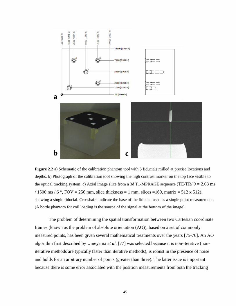
45
Figure 2.2 a) Schematic of the calibration phantom tool with 5 fiducials milled at precise locations and
depths. b) Photograph of the calibration tool showing the high contrast marker on the top face visible to
the optical tracking system. c) Axial image slice from a 3d T1-MPRAGE sequence (TE/TR/ θ = 2.63 ms
/ 1500 ms / 6 °, FOV = 256 mm, slice thickness = 1 mm, slices =160, matrix = 512 x 512),
showing a single fiducial. Crosshairs indicate the base of the fiducial used as a single point measurement.
(A bottle phantom for coil loading is the source of the signal at the bottom of the image).
The problem of determining the spatial transformation between two Cartesian coordinate
frames (known as the problem of absolute orientation (AO)), based on a set of commonly
measured points, has been given several mathematical treatments over the years [75-76]. An AO
algorithm first described by Umeyama et al. [77] was selected because it is non-iterative (non-
iterative methods are typically faster than iterative methods), is robust in the presence of noise
and holds for an arbitrary number of points (greater than three). The latter issue is important
because there is some error associated with the position measurements from both the tracking

46
system and MRI, and the spatial transformation can be estimated with greater accuracy using
more points.
The method outlined by Umeyama can be described as follows. Let Xc be a 3xN matrix
(where N is greater than 3) containing the points measured in the camera coordinate frame and
Xm be a 3xN matrix of the points measured in the MRI coordinate frame. The covariance matrix
between the two sets of coordinates can be described by
][ – [2.3]
where c and m are the mean vectors of the N points. After decomposing the covariance matrix
C by single value decomposition (SVD), C = UVDT. The rotation matrix RCM can be calculated
by
[2.4]
as proved in [77]. Once the rotation matrix has been calculated, the translation vector TCM is
- [2.5]
2.2.4 Evaluation of Calibration Accuracy
The accuracy of the calibration procedure was evaluated by positioning the fiducial
phantom in 10 arbitrary positions, approximately evenly distributed over a 5x5x3 cm space, and
applying the calculated transformation both from the camera to MRI frame and the MRI
coordinate frame to camera frame. The error was calculated as the difference between the
estimated positions (from the spatial transformation) and the true positions measured from both
coordinate frames. Utmost care was taken during camera calibration to align the camera
coordinate frame (i.e. the high-contrast checkerboard pattern) with the axis of the MRI, such that
the rotation matrix relating the coordinate systems would be confined to 90 ° rotations.

47
2.2.5 Real-Time Correction System
To update the scan plane it was necessary to calculate changes in tool position from the
tracking system data in real time. Incremental translations and rotations between time points
were estimated using the AO algorithm presented above. This is feasible because a change in
position in time is equal to a shift of Cartesian coordinate frames. The rotation matrix RCM was
decomposed into roll, pitch and yaw angles as outlined in [78], such that only 3 values needed to
be transferred to the MRI system, rather than the nine required for a 3x3 rotation matrix. The
performance of the AO algorithm was assessed using simulated motion data with noise equal to
that of the tracking system. A set of points from a static measurement of the tracking tool were
used as a basis, and incremented in x, y, and z directions to simulate motion. The AO algorithm
output was compared to the known increment inputs. The root mean squared (RMS) position
error was calculated as the root mean difference between the simulated and estimated motion
data.
The motion parameters were calculated on the personal computer (PC) housing the
camera software (Dell Dimension 9200, Intel Core 2, 2.40 GHz ) and were then transferred over
a 1GB Ethernet cable to the MRI host computer. A real-time EPI sequence was modified to
request the motion parameters and modify the gradient rotation matrix and transmit RF pulses to
adapt the slice orientation and position before the subsequent acquisition. The pipeline for the
real-time correction system is illustrated in Fig 2.3. The minimum achievable lag time between
position measurement and scan-plane update was 26 ms.

48
Figure 2.3 Illustration of the pipeline for real-time scan-plane update. Cameras track a tool situated on the
forehead of the subject. Tracking data are sent to a PC where translation and rotations of the head are
calculated. Update motion parameters are sent to the MRI MPCU for scan-plane update. See text for
details. MPCU = MR physiological measurement control unit, PC = personal computer housing camera
and server software.
2.2.6 PLACE Geometric Distortion Correction
The real-time EPI sequence was modified using the Siemens IDEA pulse sequence
programming environment such that every other volume was acquired with a k-space shift of one
phase encoding step (i.e Δky = 1/FOV), to enable PLACE geometric distortion correction [79].
Correction by PLACE was applied to each image in the time series in post-processing using
Matlab (4.2c, The MathWorks, Inc., Natick, MA) A summary of the complete analysis pipeline
for calculating a 1D pixel shift map from PLACE EPI data is described in [79]. Briefly, the
complex EPI data were multiplied together to generate a new complex image I‘. A linear phase
ramp was applied to I‘, from –π to π over the field of view, in the reverse direction to that applied
during acquisition, to generate complex image C, as given by
[2.6]

49
where, y‘ is the pixel location in the reconstructed image, from –FOV/2 to FOV/2, and y
represents the distorted coordinate along the PE direction and M1 and M2 are the magnitude
images of the EPI pair. The reverse phase ramp cancels most of the original phase ramp, leaving
behind phase data that now represents a map of pixel displacement, Δy, with
[2.7]
After the application of the linear phase ramp, the complex image C is expanded (up-sampled) in
the PE direction (e.g. from 128 pixels to 128000 pixels) by generating 100 identical copies of
each pixel to produce the image CE. This expansion is followed by smoothing in the complex
image domain, in both x and y directions using a boxcar window of 10x300 pixels, in the x- and
y-direction respectively, resulting in complex image CES. The heavy smoothing suppresses noise
in the phase data and serves as a data interpolation process to achieve subpixel warping. An
expanded, smoothed displacement map then can be calculated from CES by,
[2.8]
The distorted image is also expanded in the PE direction, without smoothing, and is corrected for
distortion on a pixel by pixel basis according to the pixel displacement map Δy. A second order
correction was applied to compensate for the concentration or dilution of signal among a smaller
or greater number of pixels in the PE direction, also known as signal ―crack up‖ or ―pile up‖. The
image intensity at each point was scaled to the local pixel shift gradient δr, by calculating the
slope of the best fit through the pixel shift values Δyn-1
,Δyn and Δyn+1. The image intensity at
each location was multiplied by (1.0 + δr) as outlined in [21]. The final corrected image was
generated by rebinning the expanded image back to its original size along the PE direction.
In the case of motion, the echo planar image pair data for PLACE correction were
selected based on the relative physical position of the object. The tracking system data were
saved and used in the PLACE post-processing pipeline to choose EPI images that had similar
positions. A difference threshold of 0.1 mm for x, y and z translations and 0.4 ° for roll, pitch
and yaw rotations were used to decide between image pairs. The search for a correction map for
an individual image began by comparing the image position relative to those of images
immediately adjacent. If neither of the adjacent images were within the threshold, the search was

50
expanded to images in the same block and then to adjacent blocks in the fMRI time series
according to the behavioral task design (see below). Images from similar blocks were used
because phase variations arising from the BOLD effect potential could be different between task
and rest conditions.
2.2.7 Evaluation of PLACE
Prior to incorporation with the real time scan plane correction the effectiveness of
PLACE for geometric distortion correction was first evaluated by applying non-linear image
registration by affine transformations in a phantom (see below) using algorithms in the Analysis
of Functional Neuroimages (AFNI) package [42]. Non-linear registration applies image
deformation, along with rigid-body transformations, to bring two images into spatial alignment.
Images corrected by PLACE and uncorrected distorted images were non-linearly registered to a
reference high resolution image acquired using a T1-weighted MPRAGE sequence not prone to
geometric distortion (TE/TR/ θ = 2.63 ms / 1500 ms / 6°, FOV = 256 mm, slice thickness = 1
mm, slices =160, matrix = 512 x 512). The non-linear registration algorithm returned scaling
factors for the x and y dimension reflecting the degree of compression or expansion required to
bring the images into alignment. Because geometric distortion for EPI can be assumed to be
substantial only in the y direction, the y-scale factor was used to compare the similarity between
the corrected and uncorrected images, and the reference image. The x-scale factor did not change
substantially when comparing images without and with PLACE correction to the reference.
Given that a scale value of 1 means that no scaling is required, the absolute scale factor was
defined by,
[2.9]
where ys is the y-direction scale factor determined from non-linear registration. Using the
absolute value allowed comparisons without consideration of whether images were stretched or
compressed. The value Sc was used to evaluate PLACE for an agar gel phantom and in vivo
images. The agar gel phantom was a cylindrical tissue-equivalent test phantom used in
subsequent experiments and was evaluated for an axial slice along the axis of the phantom.

51
2.2.8 Imaging Protocols
Functional MRI and phantom data were acquired using single-shot EPI with parameters
optimized for BOLD contrast (TE/TR/θ = 32 ms / 1000 ms / 30 °, FOV = 256 cm, slice thickness
= 2 mm, matrix = 128 x 128, 10 slices). Maps of activity were superimposed on anatomical
grayscale images acquired with T1-weighted fast three-dimensional gradient echo pulse
sequence, Magnetization Prepared Rapid Gradient Echo (MPRAGE) (TE/TR/θ = 6 ms / 35 ms /
35°, FOV = 22 cm, slice thickness = 1.4 mm, matrix = 256 x 256, 124 slices). High resolution
images of the fiducial phantom during camera to MRI calibration were also acquired by 3D
MPRAGE (TE/TR/ θ = 2.63 ms / 1500 ms / 6°, FOV = 256 mm, slice thickness = 1 mm, slices
=160, matrix = 512 x 512).
2.2.9 Phantom Design
Initial testing of PLACE and subsequent integration of PLACE with the real time scan
plane update system, was performed on a second phantom with T1 and T2 tissue equivalent
relaxation characteristics. The phantom consisted of concentric polyvinyl chloride cylinders that
enclosed two layers of agar gel doped with gadolinium diethyltriamine penta-acetic acid (Gd-
DTPA). High resolution cross-sectional images of the phantom are shown in Fig 2.4 for the
phantom placed with its long axis obtained in the right-left direction within the head coil, the
orientation used for subsequent motion experiments.

52
Figure 2.4 High resolution 3d T1-weighted MPRAGE (TR/TE/FA = 1500 ms/2.6 ms/6 °, FOV=256 mm,
Slice Thickness = 1 mm, Resolution 256x256) images of the tissue-mimicking phantom a) Sagittal; b)
coronal; c) axial orientation. Inner layer composed of white matter matched gel. Outer layer composed of
gray matter matched gel. Lines indicate slice position and orientation for axial and coronal images.
The gel layers were prepared by varying the concentrations of Gd-DTPA (Omniscan, GE
Healthcare), to modify T1 relaxation times and the concentration of Agar to modify T2
relaxation times, such that the T1 and T2 relaxation times approximated those of gray matter and
white matter at 3 T (see Table 1.1) [4]. The required concentration of Gd-DTPA and percent
composition by weight of agar were, 90 mM/L and 6.2%, and 50 M/L and 4.4%, for gray and
white matter respectively. The T1 values of the phantom tissues were estimated using a series of
inversion recovery sequences with 15 logarithmically spaced inversion times (TI) and applying
non-linear regression by equation 1.10. The estimated T1 values were 1080 ± 32ms for white
matter and 1520 ± 34ms for gray matter. Figure 2.5 shows two T1-weighted images with
inversion times set to null the signal from the white matter matched gel (a) and gray matter
matched gel (b).

53
Figure 2.5 a) T1 MPRAGE axial image of the phantom. T1-weighted inversion recovery
images: a) Inversion time TI = 750 ms, resulting in nulled white matter (WM); b) Inversion time
TI = 1050 ms, resulting in nulled gray matter (GM). White matter and gray matter layers are
outlined in yellow for clarification of image boundaries. In IR image b) the dark region
represents negative magnetization (negative values, not a lack of signal) as indicated by the
grayscale level above.
The T2 values of the phantom tissues were estimated using a multi-echo T2-weighted
spin-echo sequence and applying non-linear regression by equation 1.11. The estimated T2
values were 70 ± 3ms for white matter and 90 ± 3ms for gray matter. The T1 and T2 values were
within the bounds of their values from the literature [4]. The resulting gels were considered to be
of sufficient rigidity to approximate rigid body motion during subsequent movement
experiments. The central cylinder of the phantom was left hollow.
2.2.10 Phantom Imaging Experiments
The phantom was either imaged statically ( enabling initial testing of PLACE
performance), or moved in a complex manner by rolling the phantom up an inclined (15 ° )
acrylic ramp within the head coil using a computer-controlled MRI-compatible positioner stage

54
described previously [80-81] and push rod (Fig. 2.6). The positioner stage was capable of
making translations along one axis accurate to 2 µm at maximum velocities of 5 mm/s. To assess
the MR-compatibility of the positioner stage, the tissue-equivalent test phantom was imaged
without and with the stage present in the scanner, and tracked by the tracking system for 100
minutes duration. The positioner was not observed to introduce additional noise into the MR-
image and the tracking system stability was the same as presented in Fig 2.9. Based on initial
validation testing the tracking tool consisted of 15 markers, to reduce the position estimate error
to the level of the noise (See Results). The rolling motion of the phantom was adjusted such that
it included a translation with components in x, y and z, and rotational motion with components of
roll, pitch and yaw, thereby providing complex movement in all six degrees of freedom (6 DOF).
Figure 2.6 Photograph of apparatus for the rolling phantom experiment. The phantom was rolled up an
inclined custom acrylic ramp by a positioner stage. Physical contact was made with the phantom using a
push rod attached to the positioner. Also visible are the tracking cameras and the tracking tool consisting
of reflective spheres attached to the phantom.
During motion the phantom was scanned without and with real-time correction. The
positioner stage was programmed to simulate TCM, by actuating phantom movement in a boxcar
waveform (Fig 2.7).
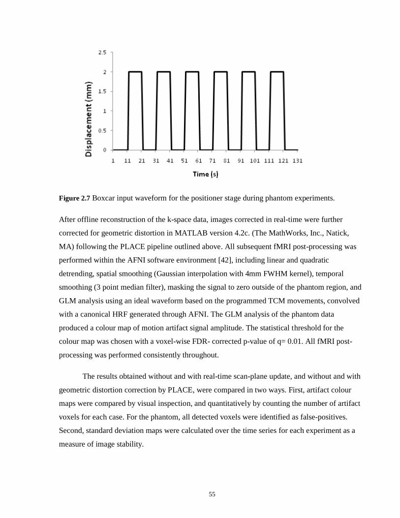
55
Figure 2.7 Boxcar input waveform for the positioner stage during phantom experiments.
After offline reconstruction of the k-space data, images corrected in real-time were further
corrected for geometric distortion in MATLAB version 4.2c. (The MathWorks, Inc., Natick,
MA) following the PLACE pipeline outlined above. All subsequent fMRI post-processing was
performed within the AFNI software environment [42], including linear and quadratic
detrending, spatial smoothing (Gaussian interpolation with 4mm FWHM kernel), temporal
smoothing (3 point median filter), masking the signal to zero outside of the phantom region, and
GLM analysis using an ideal waveform based on the programmed TCM movements, convolved
with a canonical HRF generated through AFNI. The GLM analysis of the phantom data
produced a colour map of motion artifact signal amplitude. The statistical threshold for the
colour map was chosen with a voxel-wise FDR- corrected p-value of q= 0.01. All fMRI post-
processing was performed consistently throughout.
The results obtained without and with real-time scan-plane update, and without and with
geometric distortion correction by PLACE, were compared in two ways. First, artifact colour
maps were compared by visual inspection, and quantitatively by counting the number of artifact
voxels for each case. For the phantom, all detected voxels were identified as false-positives.
Second, standard deviation maps were calculated over the time series for each experiment as a
measure of image stability.
56
2.2.11 In Vivo Experiments
Four young healthy subjects (right-handed males, average age 27 years, range 24-32
years) were recruited for this study under approval of the Research Ethics Board at Baycrest
Hospital. All subjects completed the same bilateral finger tapping tasks. After PLACE was
validated in vitro, the performance of the integrated correction technique was assessed using
block design finger tapping tasks with 9 alternating 20 s blocks of ―task and ―rest‖ conditions. A
series of five runs per subject were conducted, each with the same number of task and rest
conditions. The first run involved self paced bilateral finger tapping during the task condition.
The subsequent four runs were designed to include deliberate head motion, during which
subjects performed the same bilateral finger tapping task as the first run and in addition were
asked to perform intermittent in-plane (yaw) rotations or though-plane (roll) nodding rotations at
discrete time points. Patients were instructed to perform the deliberate head motion when given a
verbal cue. To reduce intra and inter subject motion variability, a training session was performed
by each subject at the start of each experiment, during which head position tracking data was
presented to subject as real-time visual feedback. Visual stimuli were displayed on a back-
projection screen at the entrance to the magnet bore using an LCD projector (Revolution III,
Boxlight 6000, Boxlight Corp.), and viewed by the subject using angled mirrors attached to the
head coil. The display consisted of a ―target‖ circle that would move in the horizontal direction
in response to yaw rotation and in the vertical direction in response to roll rotation. Black bars in
the horizontal and vertical direction represented yaw and roll rotations of ± 2 ° and ± 2 °
respectively. Prior to training, subjects were instructed to rotate their heads such that the target
circle would remain within the boundaries set by the black lines. Some patients deviated from the
instructed path and overshot their rotations during the session. For some individuals the deviation
was substantial enough as to obscure tracking points from the cameras. In such cases the current
session was stopped, training was administered and the session repeated. To improve
performance, a second training procedure was provided where the visual output of the tracking
cameras themselves, was presented to the subject. Subjects were able to see their head motion as
it appeared in the cameras with respect to the head coil. This added level of training was
effective at improving performance and quickly adopted for cases that had difficulty in following
57
the instructed path when only given preliminary training. After training, each fMRI experiment
involving head motion was repeated without and with real-time correction.
For the in vivo experiments, the data were analyzed by the same post-processing pipeline
used for the phantom experiments (as outlined above), with the distinction that in this case
activation maps were generated as a result of GLM analysis, rather than color maps of false
positive motion artifact. For each fMRI experiment, the results obtained without and with real-
time scan-plane update, and without and with geometric distortion correction by PLACE, were
compared in two ways. First, activation images were compared by visual inspection and
quantitatively by plotting the number of detected activated voxels in either the sensory motor
cortex (SMC) as a measure of true-positives, or outside of the SMC as a measure of false-
positives. For each individual, the SMC region of interest was selected based on neuroanatomy
(known location and approximate extent of the SMC) and the location of the active regions
observed during the reference task. The shape and size of the SMC region of interest was unique
for each individual. Second, standard deviation maps were calculated over the time series for
each experiment as a measure of image stability. In addition, the results for each experimental
condition were compared across all subjects.
2.3 Results
2.3.1 Validation of the Tracking System
The accuracy of the tracking system was taken to be the smallest displacement step size
such that plot between the measured versus applied translations would have a linear fit with
slope 1.00 ± 0.01. The evaluated translation accuracies and precisions were 30 ± 20 µm, 20 ± 20
µm and 40 ± 10 µm for x, y, and z, respectively (Fig 2.8).

58
Figure 2.8 Tracking system accuracies in x, y and z measured inside of the magnet bore. The fit of each
line yields a slope of 1.00 ± 0.01, giving accuracies and precisions of 30 ± 20 µm, 20 ± 20 µm and 40
± 10 µm for x, y, and z, respectively.

59
2.3.2 Tracking System Stability Results
The standard deviation of the radial position over the course of the experiment was found
to be 20 ± 10 µm and the RDR was determined to be 6µm/hr, (Fig 2.9), suggesting that the
tracking system remains stable for epochs on the order of a typical fMRI session (approximately
1 hr).
Figure 2.9 Radial position of a static tracking tool over time. The radial position is seen to
remain stable over the course of 100 minutes, with a radial drift rate of 6µm/hr.
2.3.3 Accuracy of Coordinate Transformation
The resulting mean error between measured and calculated positions over 10 trials, based
on use of the fiducial phantom and 40 calculations, was found to be 80 ± 20 µm, 70 ± 20 µm and
110 ± 50 µm for x, y, and z, respectively. The heightened discrepancy does not reflect tracking
system error, but is likely due to the error in measuring position from the MR images. Because

60
the transformation between the camera and MRI coordinate frames involves only a translation
and rotation and does not include a change in scale, the displacements measured in the camera
coordinate frame will have the same magnitude in the MRI coordinate frame after
transformation. Given only linear offsets from the true origin of the MRI system, the tracking
error will not be affected. However inaccuracies in the coordinate transformation matrix will
contribute to the tracking error when there is substantial misalignment between the coordinate
frames due to inaccurate rotation matrix estimates. The misalignment will result in a
redistribution of vector components, for example, a translation in z only, may be transformed
such that it has components in x and y. Again, the magnitude of the vector will remain the same,
but the contributions from components may change. Therefore, the mean calibration errors
quoted above do not affect the tracking error in a linear additive fashion, but in a more subtle
manner. In all of the experiments subsequently performed, errors in coordinate transformation
were not found to be a substantial limitation.
2.3.4 Real-Time Tracking
The RMS position error decreased with an increasing number of points used for
calculation. The error was reduced to the magnitude of the noise when using 10 points or more as
shown in Fig 2.10. The transformation calculation speed was found to be linearly dependant on
the number of points, with an operating time of approximately 1ms for 10 points on a Dell
Dimension 9200 (Intel Core 2, 2.40 GHz ).
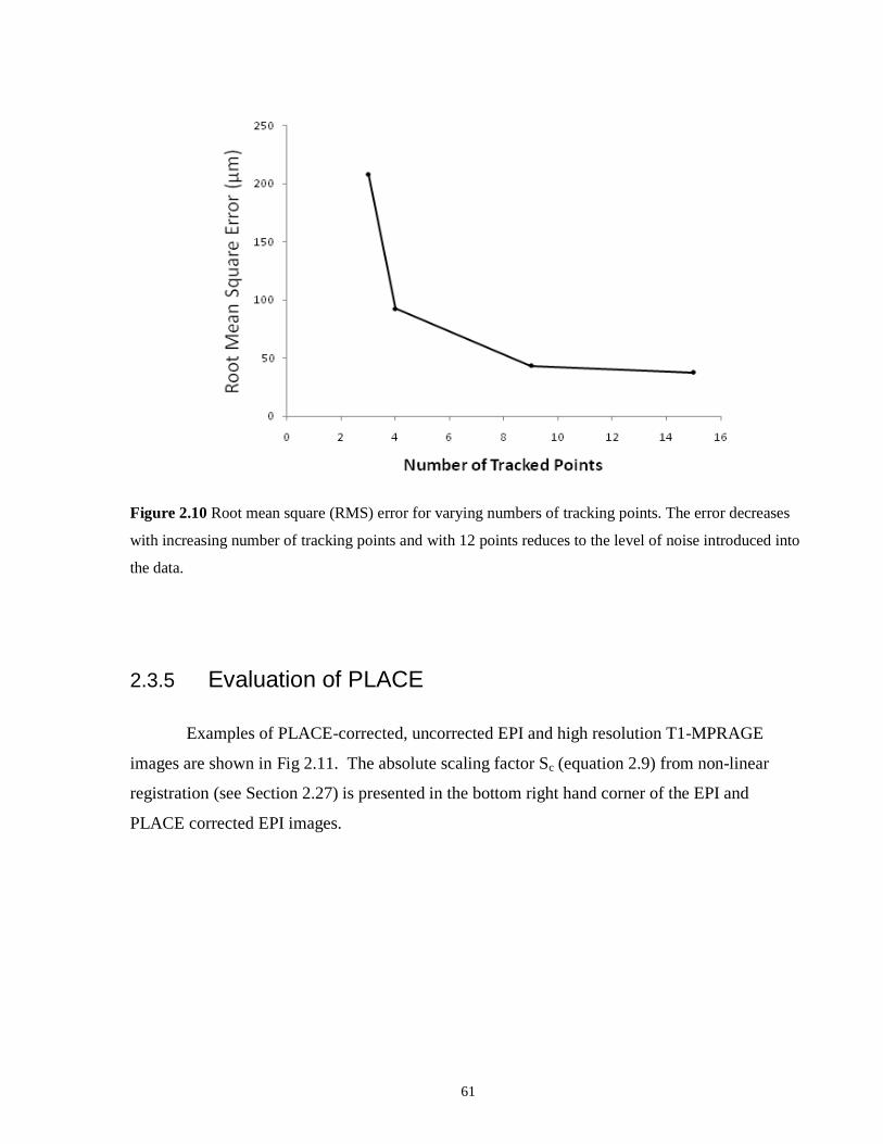
61
Figure 2.10 Root mean square (RMS) error for varying numbers of tracking points. The error decreases
with increasing number of tracking points and with 12 points reduces to the level of noise introduced into
the data.
2.3.5 Evaluation of PLACE
Examples of PLACE-corrected, uncorrected EPI and high resolution T1-MPRAGE
images are shown in Fig 2.11. The absolute scaling factor Sc (equation 2.9) from non-linear
registration (see Section 2.27) is presented in the bottom right hand corner of the EPI and
PLACE corrected EPI images.

62
Figure 2.11 High resolution, EPI and PLACE corrected EPI for: a cylindrical agar gel phantom
(top row) and an in vivo brain image slice (bottom row). The value of the absolute scale factor
Sc, from non-linear registration (see Section 2.27) is indicated in the bottom right hand corner.
Signal associated with Nyquist ghosting, visible in the uncorrected images, can be seen to
have been corrected using PLACE. Images corrected by PLACE had consistently smaller
absolute y scaling factors (Sc), when registered to a high resolution image, compared to
uncorrected images. The Sc value for PLACE correction was approximately one order of
magnitude less for both phantom and in vivo cases. The effect also was obvious by visual
inspection.

63
2.3.6 Phantom Experiments
The six motion parameters measured by the tracking system over the course of a
representative rolling phantom experiment are shown in Fig 2.12. The motion was seen to
contain contributions from translation in x, y and z directions and rotations in roll, pitch and yaw.
The motion was measured 8 times to test reproducibility. The mean change and standard
deviation for each motion parameter were 1.10 ± 0.01 mm, -1.30 ± 0.03 mm and 4.50 ± 0.01 mm
for x, y, and z translations and 1.8 ± 0.2°, 0.8 ± 0.1°, and 1.2 ± 0.2° for roll, pitch, and yaw
rotations respectively. Translations in figure 2.12 are displayed in centimeters to illustrate the
contributions from x, y, and z directions simultaneously on one graph.
Figure 2.12 Representative translation data in millimeters (top) and rotation data (bottom) as measured
by the tracking system during a rolling phantom experiment. The phantom is driven in a boxcar waveform
with contributions from x, y and z displacements and roll, pitch and yaw rotations.

64
Figure 2.13 shows representative artifact color images overlaid on an axial MPRAGE
grayscale image of the phantom (top row), times series data from a representative anterior gray
matter voxel, identified by the cursor (middle row) and standard deviation maps (bottom row) for
a) motion without correction; b) motion with real-time correction; and c) motion with real-time
correction and PLACE. In the case of motion with no correction, the artifact color map shows a
large number of statistically significant false-positive activations, and representative time series
data are seen to fluctuate at large amplitude as the phantom undergoes boxcar motion. In the case
of motion with real time correction, there are less numerous false-positive activations with
statistically significant t-scores and the associated changes in signal intensity in the time series
data are attenuated. The artifact colour maps in a) and b) show artifacts that lie outside the
phantom boundary as a result of geometric distortion. When the data from real-time correction
are further corrected for geometric distortion using PLACE, very few locations of artifact
remain.
Motion artifact voxel counts over the five runs are shown in Table 2.1 for a) a static
reference; b) motion with no correction; c) motion with real-time correction; and d) motion with
real-time and PLACE correction. The trend for each run is consistent with representative data
shown in Fig 2.13. In the case of motion with real-time correction, the number of detected voxels
is substantially less than for the case with motion with no correction. When real-time correction
and PLACE are combined, almost no artifact remains within experimental error. It can be seen
that the intensity of the standard deviation map is reduced with real-time correction, compared to
the case of no motion correction, and further reduced with the application of PLACE. In the
latter case, elevated standard deviation is primarily located immediately adjacent to boundaries
with differing signal contrast.

65
Figure 2.13 Motion artifact color maps (top row), and time series data from a representative voxel in the
anterior gray matter layer (middle row) and standard deviation maps (bottom row) for the case of a)
motion with no correction; b) motion with real-time correction; and c) motion with real-time correction
and PLACE. The number of artifact voxels decreases with the use of real-time scan-plane update and is
further improved with the addition of dynamic geometric distortion correction. Motion-induced artifactual
signals are reduced when using real-time scan-plane update with geometric distortion correction by
PLACE.

66
Run Reference Motion
(No Correction)
Motion
(Real-Time Correction)
Motion
(Real-Time Correction + PLACE)
1 0 827 202 15
2 0 746 161 3
3 0 791 194 19
4 0 921 245 44
5 0 873 213 29
Mean 0 821 201 20
Standard Deviation 0 74 35 17
Table 2.1 Artifact voxel counts for a) a static reference; b) motion with no correction; c) motion with
real-time correction; and d) motion with real-time and PLACE correction over five runs.
2.3.7 Bilateral Finger Tapping
The six motion parameters measured by the tracking system for an individual
representative subject over the course of two finger tapping experiments are shown in Fig 2.14;
a) finger-tapping with intermittent in-plane motion; b) finger-tapping with intermittent through-
plane motion. The mean rotation angles and standard deviations, for the four subjects were 1.3 ±
0.4° and 1.5 ± 0.5° for roll and yaw during the through-plane motion and in-plane motion
experiments, respectively. Translations in figure 2.14 are displayed in centimeters to illustrate
the contributions from x, y, and z directions simultaneously on one graph.

67
Figure 2.14 Motion parameters for fMRI of a single representative subject performing a bilateral finger
tapping task with intermittent in-plane motion (left) and through-plane motion (right). Motion was cued
by the experimenter during rest periods of the block-design finger tapping experiment.
Functional MRI results from representative bilateral finger tapping experiments from the
same subject are presented in Fig 2.15. Activation images, time series data from a representative
voxel in the primary sensory motor cortex (SMC), and temporal standard deviation images are
presented for each case: a) no motion, b) motion without correction; c) motion with real-time
correction and d) motion with real-time and PLACE correction, for in-plane motion and for
through-plane motion. In the case with no deliberate motion, modest motion was detected even
when the subject focused on remaining still. Typical activation patterns, as shown in the time
series data, were detected bilaterally in the SMC. In the case of in-plane or through-plane motion
with no correction, signal intensity changes within the time series were seen to occur
synchronously with motion. The activation maps show an increase in the number of false-
positive activations outside of the SMC, particularly around the edges of the brain for the case of
in-plane motion and within the frontal lobe for the case of through-plane motion. In addition, the
number of voxels identified as active within the SMC was reduced compared to the case with no
motion. In the case of in-plane motion with real-time correction, motion-synchronous changes in

68
signal intensity were still visible in the time series data, but attenuated with respect to the no
correction case. The activation maps show reduced false-positive activations outside of the SMC
areas and an increase in the number of activations detected within the SMC areas compared to
the case with no correction. When the data from the real-time correction case are further
corrected for geometric distortion using PLACE, the spurious changes in signal intensity over
time are further attenuated so that the time series data strongly resemble those for the static case.
The activation image also includes fewer instances of false-positives and has an increase in the
number of voxels identified in SMC areas. The activation patterns more closely resemble the
static case compared to the case with real-time correction only, and have shifted slightly anterior
due to the geometric distortion correction. It can be seen that the intensity of the standard
deviation maps is reduced with real-time correction, and further reduced with the application of
geometric distortion correction for both cases, such that they resemble those for the static case.

69
Figure 2.15 Activation maps (top row) and time series of a representative voxel in the primary sensory
motor cortex (SMC) (middle row) and standard deviation maps (bottom row) for: a) reference case of
minimal head motion (no motion correction); b) motion with no correction; c) motion with real-time
correction; and d) motion with real-time and PLACE correction. Arrows indicate the location of motion
related signal change.

70
The number of activations over all four subjects are shown in Table 2.2: a) through-plane
motion; and b) in-plane motion, in the SMC and regions exterior the SMC for: a) reference case
of minimal head motion (no motion correction); b) motion with no correction; c) motion with
real-time correction; and d) motion with real-time and PLACE correction. The group trend is
similar to the trend observed for the individual case presented above. The number of activations
observed in the SMC decreased in the case of motion with no correction, for both the in-plane
rotation and nodding cases. There were consistently fewer detected voxels for the nodding case
then for the in-plane case. For the case of motion with real-time correction, the number of
detected voxels increased for both the in-plane rotation and nodding cases. After the data were
further corrected for geometric distortion, the number of detected voxels in the SMC increased,
and reached values close to those observed for the reference case. The number of detected voxels
in the SMC was consistently lower for the nodding case compared to the in-plane rotation case.
For regions outside of the SMC, the number of false-positives increased substantially in
the case of motion with no correction, in comparison to the fMRI data acquired with minimal
head motion. The number of false-positives was consistently larger for the nodding case than for
the in-plane rotation case. In the case of motion with real-time correction, the number of false-
positives outside of the SMC decreased in comparison to the case of motion with no correction,
remaining larger in the nodding case than in the in-plane rotation case. Data further corrected for
geometric distortion correction shows a decrease in the number of false positives compared to
the case with real-time correction only, approaching the reference condition.

71
A Through-Plane Motion
SMC Exterior
Subject Reference
Motion
(No
Correction)
Motion
(Real-Time
Correction)
Motion
(Real-Time Correction
+ PLACE)
Reference Motion
(No Correction)
Motion
(Real-Time
Correction)
Motion
(Real-Time Correction
+ PLACE)
1 178 2 42 103 0 427 274 2
2 181 8 82 140 5 522 219 23
3 224 11 112 194 20 662 317 35
4 180 6 71 142 10 544 285 18
Mean 191 7 77 145 9 539 274 20
Standard Deviation 22 4 29 37 9 97 41 14
B In-Plane Motion
SMC Exterior
Subject Reference Motion
(No Correction)
Motion
(Real-Time Correction)
Motion
(Real-Time Correction +
PLACE)
Reference Motion
(No Correction)
Motion
(Real-Time Correction)
Motion
(Real-Time Correction +
PLACE)
1 178 38 59 151 0 152 27 5
2 181 73 87 176 5 191 76 12
3 224 89 103 206 20 238 89 20
4 180 77 85 191 12 214 82 16
Mean 191 69 84 181 9 199 69 13
Standard Deviation 22 22 18 23 9 37 28 6
Table 2.2 The number of activations over all four subjects for: A) through-plane motion; and B) in-plane
motion experiments, in the SMC and regions exterior to the SMC for: a) reference case of minimal head
motion (no motion correction); b) motion with no correction; c) motion with real-time correction; and d)
motion with real-time and PLACE correction.
2.4 Discussion
In this study, a method for real-time scan plane update with integrated geometric
distortion correction by PLACE was developed and evaluated. The approach was developed to
correct for three motion artifacts in fMRI data, slice misalignment, non-linear spin-history

72
disruption and dynamic magnetic field distortion. Data obtained on a tissue-equivalent test
phantom undergoing complex motion and four healthy human volunteers showed substantial
improvement when using the integrated correction approach, in the case of deliberate motion,
compared to no correction and real-time correction alone. The ramifications of this work are
discussed below.
The accuracy and precision of the in-bore optical tracking system was evaluated to be
better than 40µm and 0.1° for translation and rotation respectively as seen in Fig 2.8. These
results are comparable to the best accuracies reported by other recent implementations of optical
tracking systems [66-68]. The RMS error of the tracking system was seen to decrease with
increasing number of tracking points, such that the error was reduced to that of simulated noise
with 12 points or more (Fig 2.10). This result advised the optimum number of tracking points for
further experiments. The tracking system was shown to be highly stable for epochs for a typical
fMRI session, with a radial drift rate of 6µm/hr (Fig 2.9). The accuracy, precision and stability of
the tracking system were sufficient for real-time update at 3T, where typical fMRI voxel sizes
are on the order of 1-2 mm. Optical tracking systems with comparable accuracy may of be
substantial interest to further development of applications at 7T and higher, where image
resolution can be on the order of hundreds of microns [82]. Because the stereo 3D reconstruction
accuracy depends on the relative angle and distance between the two cameras, the optimized
setup for the two cameras could be explored further to enhance accuracy.
The tracking tool position was measured with respect to the camera coordinate frame and
had to be transformed to the MRI coordinate frame. A calibration phantom was constructed with
5 points visible to both the tracking system and MRI for estimating the transformation between
coordinate frames using a closed form AO algorithm (Fig 2.2). To improve the accuracy of the
estimate, the phantom was positioned in three locations for a total of 15 points per coordinate
frame, based on the validation of RMS error with the number of tracking points. The error of the
calibration procedure was estimated by finding the difference between the positions of points in
one frame and using a previously calculated transformation to rotate and translate the data into
the opposing frame. The estimated errors were 80 ± 20 µm, 70 ± 20 µm and 110 ± 50 µm for x, y
and z directions respectively. Because the magnitude of displacements stayed constant from one
coordinate frame to the other, calibration error was a negligible contributor to overall tracking
error. Improvements to the calibration phantom could include more points, such that the

73
calibration measurements need only be taken once, saving time and potentially improving
accuracy. A previous publication [66] used a high resolution phantom with well ordered
structures to provide more points for measurement, such that repeat scans were not necessary,
however, the reported calibration accuracy was similar to the results presented here. In this work,
the tracking cameras were not permanently situated within the magnet bore, such that camera
calibration and camera to MRI coordinate frame calibration had to be repeated at the start of each
experimental session.
The tracking system presented here has several practical advantages compared to other
implementations of real-time scan-plane update. Compared to MR-based methods, including
ONAV, SNAV and active-markers, the optical tracking system does not increase scan time
during fMRI, or constrain the choice of pulse sequence. In addition, optical tracking has
demonstrated higher accuracy and temporal resolution. The MR-based active makers used in the
integrated real-time scan-plane update approach presented by Ooi et al., doubles the effective
scan-time and has substantially poorer accuracy. The optical tracking system also has the
advantage that it operates in the infrared spectrum, such that fMRI experiments that include
visual stimuli do not interfere with the tracking system measurements, and vice versa.
There are several potential concerns when considering use of an in-bore tracking system,
such as potential electromagnetic interference caused by tracking system electronics. The
influence of the tracking system on fMRI was assessed by imaging a static standard Siemens test
phantom without and with the tracking system in-bore and active. No signs of interference were
observed with the tracking system in place, suggesting that the effect of the tracking cameras on
fMRI was negligible. However, MRI compatibility should be assessed intermittently as routine
quality assurance. A second issue is that the optical tracking system requires a clear line-of-sight
to the tracking tool at all times. This introduces some restrictions on the placement of the
tracking system with respect to the subject and fMRI hardware. For example, the 12 channel
head coil was used for the tracking cameras presented here, compared to a 32 channel head coil,
to provide a clear line of sight for the tracking system. However, it should be possible to
incorporate this requirement by introducing optical windows into future high channel count coil
designs.

74
For in vivo experiments, the number of tracking points used varied by subject to
maximize the number of tracking points within the field of view. For example, subjects with
smaller profiles and that had their foreheads farther from the cameras, required larger tracking
markers used in greater number. On the other hand, patients with larger heads required fewer and
smaller markers.
Software was written to handle real-time calculation and transfer of motion estimates to
the MRI system, where it was integrated into a real-time EPI sequence. A 1Gb Ethernet was used
for data transfer such that the latency between position measurement and scan-plane update was
~26 ms, which is comparable to the shortest lag times reported in the literature of any real-time
update system, either by MR-based methods or optical tracking [64-68]. It is anticipated that as
MRI system technology continues to advance, this lag time will eventually reduce even further.
The implementation of geometric distortion by PLACE was validated by non-linear
registration (Fig 2. 11), and was demonstrated to correct phantom and in vivo data, such that they
were quantitatively closer to a high resolution reference than uncorrected images. Geometric
distortion correction by PLACE has several advantages compared to other techniques that have
been integrated into real-time correction systems. Compared to the phase difference technique
[21, 69], it does not require phase unwrapping, and provides absolute, rather than relative
geometric distortion correction. In contrast to field estimation techniques based on susceptibility
maps, PLACE is simpler to implement and is based on a direct measure of field distortion rather
than a model based estimate. In addition, PLACE is able to correct for Nyquist ghost artifacts
simultaneously, that otherwise require a separate correction technique. The real-time sequence
was simply modified to enable PLACE, such that geometric distortion correction could be
applied uniquely for each head position, by using the position data from the tracking system to
pair images based on their relative position. In the experiments where time series contained
several hundred images, position matching was almost always successful in finding a suitable
correction map. In the cases where position matching could not be achieved, correction maps
obtained from other nearby pairs were used, that resulted in similar quality correction.
Geometric distortion is typically corrected for using a field map acquired at the beginning
of the scan and applying the resulting correction to all images in the time series irrespective of
head position. The integrated approach presented here generates a unique correction map for

75
each head position, providing more accurate geometric distortion correction that compensates for
dynamic changes in field inhomogeneity. Furthermore, geometric distortion correction is
simplified to a one-dimensional problem by real-time scan plane update, because the anatomy is
locked with respect to the phase-encode direction.
2.4.1 Phantom Experiments
Excellent correction was achieved over complex 6DOF motion. Comparing the activation
map and time series data from Fig 2.13 for the case of motion without and with real-time
correction, the latter was seen to attenuate the motion-induced signal changes, and substantially
reduce the number of false-positives. Many significant voxels were still identified however, even
when using real-time correction. Residual signal deviations co-incident with motion were also
visible in the time series. This may have resulted from several factors including the effect of
position dependant geometric distortion and subtle changes in B1 amplitude and phase, which
remain to be investigated. Finite lag may have also be a cause, as update latency can result in the
incomplete suppression of spin-history transients. From equation 1.), given a latency of 26 ms,
slice thickness of 2 mm and a mean speed of 3 mm/s, based on the position tracking data, the
theoretical maximum artifact amplitude as a percent of signal change from baseline was found to
be 3.9 %. From Fig 2.13, this predicted percentage change is similar to what is observed in the
case of motion with no correction. Rarely, the finite lag resulted in scan plane correction
occurring after motion.
The cause of the negative ‗transients‘ in the phantom experiments (Fig 2.13) was a slight
overshoot of the phantom target position. When rolling the phantom up the acrylic ramp, the
phantom rolled slightly further than the specified target input, due to the momentum given to it
by the positioner, before rolling back down the ramp and making contact with the push rod.
Given the short, yet finite lag time, this overshoot was measured and used to update the scan
plane, resulting in the appearance of overcompensation once the phantom had settled back to its
target position. This effect would be reduced if the angle of the ramp were increased, such that
more force would be required to overshoot the target position. In our setup, the ramp angle was
constrained by the diameter of the phantom and the tracking system FOV. The issue would also

76
be partially resolved by using slice by slice, rather than volume by volume correction. Whereas
some slices would be affected by the overshoot, because the phantom rests at the target position
for a substantial duration (10 s), most slices would be correctly updated. The improvement
provided by slice by slice versus volume by volume scan plane correction would carry to other
types of motion, such as fast transient motion, where only some slices would be affected rather
than the entire imaging volume.
Based on the results from the subsequent application of PLACE it would appear that
geometric distortion may be the most significant contributor to the number of false-positives, that
remain in the case of motion and real-time correction, as the number of detected voxels decreases
significantly after geometric distortion correction compared to the case of real-time correction
only. This is also supported by the substantial distortion seen in the uncorrected EPI images.
With regards to the uncorrected case, the geometric distortion resulted in large deviations
between the grayscale structural image and the artifact maps, such that many false-positive
voxels were detected outside of the phantom volume. After geometric distortion correction the
artifact maps conformed to the phantom structure and all artifact was observed within the
phantom.
Although the phantom motions were highly reproducible, there were variations in the
number of false-positives detected in each case (Table 2.1). This variation may have resulted
from several sources including the tracking error and the error due to finite lag. Based on the
output motion parameters, each experiment did not receive precisely the same position update
values, however the cumulative position change was the same. This implies that the tracking
system had the same accuracy in each case, however, the motion was being sampled at different
times. Indeed, the positioner stage was triggered manually, such that the timing for each
experiment was not identical between runs. This variable timing could explain some of the
variation in detected false-positives. It should be noted that the inter-run variability was the
lowest in the case of real-time and geometric distortion correction, suggesting that there may be
other interactions, associated with field non-uniformity that may have contributed to the
variability that were subsequently corrected.
Previous work has been published on real time correction with test phantoms [62, 66, 68].
This work however, included the first use of a tissue-equivalent test phantom for evaluating a
77
real-time system in an integrated correction approach. Tissue-equivalence was particularly
advantageous for investigating the effect of motion on the appearance of spurious activations.
This is also the first inclusion of reproducible, complex motion with 6DOF. Previous published
work has involved phantoms undergoing stepwise or continuous motion, in one degree of
freedom only [62, 68]. Qin et al, presented a more complex motion, with x, y and z components,
performed manually.
2.4.2 Finger Tapping Experiments Without and With Tracking
As opposed to the phantom case, the functional MRI experiments involved incidences of
true activation that could also be compared between each case in addition to the number of false-
positives. Comparing the activation maps and time series for the reference case and motion
without and with real-time correction, the latter was seen to attenuate the motion-induced signal
changes, and reduce the number of false-positives compared to the reference case. Broadly, the
number of false-positives was significantly greater in the case of through-plane compared to in-
plane motion. In addition the number of voxels within the SMC was much smaller for the case of
nodding compared to in-plane rotation (Table 2.2 A) and B)). The location of false-positives in
the activation maps reflects the nature of the rotations. For in-plane rotation, false-positive
activations appeared predominantly around the edges of the brain, and in the midline between the
left and right hemispheres. For the nodding case, most of the false-positives were found either in
the frontal and occipital lobes.
The precise timing of each rotation, with respect to the experimental paradigm, was not
constant, as it was advised to the patient manually through the intercom between the console and
scan-room. This difference in timing is evident in both the time series and displacement graphs
between the cases without and with real-time correction. Reaction time, in addition to the
subject‘s level of concentration, may have also played a factor in the timing discrepancy, and
likely added some contribution to the variability between subjects. The rotations occurred during
resting periods, chosen such that the underlying BOLD signal fluctuations were left intact for the
purpose of comparison, and that the motion would not interact with other signal as to be clearly

78
visible. Further investigation of rotations during other periods of the paradigm may be helpful in
investigating the effect of real-time correction.
Again, many significant voxels were identified even when using real-time correction, for
both cases. In the nodding case, however, the number of false-positives was substantially greater
than for in-plane rotation. This is likely because nodding involves a change in head orientation
with respect to the main magnetic field causing discrepancies in field uniformity that would not
be expected to occur in the case of in-plane rotation. The most susceptible regions to geometric
distortion at the location of the SMC along the superior-inferior axis are the frontal and occipital
lobes, as evidenced by field maps [21]. Indeed this observation may be supported by the location
of the majority of false-positives in the nodding case. That field non-uniformity is the cause of
the residual false-positives is further supported by their subsequent reduction after applying
geometric distortion correction to the real-time corrected data in the nodding case (Table 2.1 A)).
Although there is also a reduction in false-positives in the in-plane rotation case, the effect is
more subtle than for nodding and may be in part due to the small changes in orientation of the
head with respect to the main magnetic field as a result of yaw rotation (i.e. the rotation is not
perfectly in-plane). As can be seen from the comparison between uncorrected and PLACE
corrected EPI images (Fig 2.11), the SMC is subject to less geometric distortion than locations in
the frontal lobe, such that the location of the SMC activation shifted only slightly with respect to
the reference. For the subject presented, this did not result in discrepancies in the choice of the
region of interested, however it was seen to have a noticeable effect on voxel counts for some
subjects.
2.4.3 Group Overview
Excellent correction results were achieved over 4 healthy adults (Table 2.2 A) and B)).
The trends identified for the individual data presented were consistent between subjects, in that
the number of false-positives was the lowest in the case of real-time and geometric distortion
correction, accompanied by an increase in the number of true activations detected in the SMC.
Inter subject variability had a significant effect on the number of detected voxels identified in the
activation histograms both within and exterior to the SMC, first because individuals had different

79
degrees of activation when performing finger tapping, and second due to differing SMC
morphology. For example, subjects that had narrow SMC morphology had fewer activated SMC
voxels per slice, and more slices with activity than did those subjects with wider morphology. In
addition, there was some variability in the slice positions, again somewhat dependant on inter-
subject morphological differences. There was larger variation in the number of false-positives
detected in the nodding case compared to in-plane rotation. Because the angle of rotation was
guided and had relatively low inter-subject variability, this observation is likely due to
differences in head geometry and the influence of magnetic field non-uniformities with changing
orientation.
As noted, inter-subject variability affected the number of tracking points that could be
reliably tracked during an experiment. Interaction between patient head size and the effective
FOV of the cameras resulted in changing the number of markers. Over the course of the
experiments several different tracking tools were developed, each designed to be optimized for
the maximum number of visible tracking markers based on head morphology. Because RMS
accuracy depends on the number of tracking points (Fig 2.10), there was some slight variability
in the tracking accuracy for each subject, however, the number of markers was maintained
consistently above 10.
In general, the positions of activation loci were shifted after geometric distortion
correction. In particular, the SMC voxels were shifted slightly anterior. For several subjects, this
had a modest effect on the voxel count within and outside of the SMC region of interest. For two
subjects, the change in SMC position resulted in an increase in the number of detected voxels
within the region of interest. In one case, the shift resulted in a slight decrease in the region of
interest, and an increase in the number of voxels identified as being false-positives. Again, this
involved an interaction between inter-subject variability in head and brain geometry, and the
resulting variations in geometric distortion.
One limitation of the experiments presented here, is that they dealt only with overt
deliberate motion at discrete time-points, in a step-wise fashion. This provided a clear means to
compare time series between cases without and with correction, however a full characterization
of the performance of the system in the case of continuous random movement still needs to be
investigated. Previous work has been published examining several types of motion in the context

80
of real-time correction, including breathing-related motion [66], stepwise rotations and
translations [62, 66], slow continuous rotation and translation [63, 66, 68] and fast back and forth
rotational motion [68]. Experiments performed on patient populations of interest using the
integrated correction system would also be a useful progression for this initial investigation.
Currently, no application of real-time correction or an integrated geometric distortion approach
on patient populations has been reported.
The integrated approach presented here uses position information to select pairs of
images to use for PLACE geometric distortion correction. Although most often adjacent images
could be used, the case did occur where both possible choices of correction map did not result in
an accurate correction (e.g. the current image and the image before and after were taken at
different positions). To remedy this, rather than enforcing a binary choice between two possible
correction maps, position data was used to find a match between the current image and any other
image with an opposed phase ramp located at or near the same relative position, as close as
possible to the current image in the time series. The constraint on the time series position was
enforced such that the BOLD response was maintained for fMRI analysis. In the case when no
pairs could be found, images were corrected using maps generated for other image pairs from as
close as possible within the time series and within the same block. This method was chosen
because although distortion correction was typically adequate by inspection when using maps
further apart in the time series (for example in an opposing block), changes in phase induced by
BOLD dephasing appeared to cause discrepancies in the distortion correction and the resulting
time series. On average (N=8, 4 nodding, 4 shaking), in a time series with 180 images, a search
was conducted outside of adjacent images 17 times and a replacement from an adjacent block
was required 4 times. This low rate of replacement may be due to the controlled subject motion
in the experiments and might be expected to be larger for experiments with continuous random
motion.
2.4.4 Improving Integrated Correction and Future Applications
Despite the demonstrated effectiveness of real-time scan-plane update, the method relies
on the assumption that the brain behaves as a rigid body. However, the brain is not a rigid body

81
and is known to be pulsatile, with shifts on the order of 500 µm at the brainstem in time with the
cardiac cycle, 10-20% of which is transmitted to the cerebral cortex [83]. This deformation
represents the ultimate limit to real-time scan-plane update, as well as any other methods that
make the assumption of rigid body motion. Furthermore, this slight shift will have an effect on
PLACE geometric distortion correction as movement between images will result in errors
comparing phase values.
Some suggestions as to how to improve the integrated correction technique have been
mentioned throughout the discussion. Firstly, although the tracking system has high accuracy,
finite lag and coordinate frame transformation, introduce error into the motion update
parameters. The system was optimized to a 26 ms lag, which is comparable to best reported lags
achieved by other groups [66-68], however this lag time can still lead to position discrepancies of
2-10 µm, depending on velocity. Excursions of 10 µm may still result in substantial signal
changes particularly at boundaries between tissue types. A decrease in the lag time would
necessarily increase the accuracy of the real-time update system and further optimization may be
worth future attention. Effort was made to optimize the accuracy of the calibration procedure as
well as reduce the time necessary to complete it before experimental sessions. Error inherent in
measuring positions using MRI images, and the finite error of the tracking system itself
contribute to discrepancies in the transformation between coordinate frames. Although the
update system deals with changes in position, such that relative displacements are maintained,
errors are expected to occur when the axis of rotation for subjects differ substantially from that of
the MRI, as might be the case for pediatric patients [33]. The observed performance of the real-
time update system implies that the error was not substantial for the adult subjects tested.
Nonetheless, fine tuning of the transformation parameters with knowledge of the various
coordinate frames can be performed to compensate for calibration errors (i.e. offset vectors to
compensate for low profiles in pediatric patient populations).
The method for geometric distortion correction used here, has some limitations in that it
cannot correct for signal loss due to severe dephasing, as evident from the examples provided of
corrected and uncorrected EPI images. Loss of signal around areas of larger magnetic field
inhomogeneity can be a significant issue when investigating neural activity in the frontal lobe,
lateral temporal lobes and posterior occipital lobe. Correction for signal loss within the
framework of real-time scan-plane update has received little treatment in the current literature,

82
but may warrant further attention to move towards a more complete correction strategy. Real-
time Z-shimming, where the z gradient is actively shimmed during scan-time to reduce intra-
voxel dephasing [84] is one possible avenue that could potentially work within a real-time scan-
plane update framework and preserve phase ramp information in the PE direction for PLACE
geometric distortion correction. Higher order magnetic field shimming (greater than 2nd
), can be
performed to reduce overall field non-uniformity and reduce signal loss due to dephasing both
in-plane and through-plane [85-86]. While this would offer an improvement, perfect shimming
for one head position, will not ensure magnetic field uniformity in the case of head motion.
Dynamic shimming, with or without z-shim, which involves performing low order, frequent
shimming can compensate for changing field non-uniformity due to head position [87]. Another
method is to use designer RF pulses, coupled with parallel transmit excitation, to enforce
uniform in-plane excitation [88]. However, the performance of the above techniques deteriorates
in the presence of head motion and would benefit from an integrated real-time correction
solution.
2.5 Conclusions
An integrated motion correction approach has been presented using real-time scan-plane
update by optical tracking and geometric distortion correction by PLACE for fMRI. Results
obtained in phantom and in vivo experiments indicate that more robust activation maps can be
generated when using real-time and geometric distortion correction compared to real-time
correction alone. Despite the success of real-time scan-plane update there are cases for which
residual errors, due to dynamic geometric distortion, remain in the data. The work here suggests
that such errors can be effectively suppressed using PLACE geometric distortion correction
guided by head position data. Further investigation is required to develop a complete
characterization of the integrated approach for all types of motion and in relevant patient
populations. Hopefully, this future work will play a role in increasing the use of fMRI in patient
populations and for clinical applications.
3

83
Chapter 3
Conclusions and Future Directions
3.1 Summary
The work presented in Chapter 2 supports the hypothesis that real-time scan-plane update
by optical tracking with integrated geometric distortion correction by PLACE provides improved
correction of motion artifacts over real-time alone, due to correction of effects relating to
dynamic magnetic field non-uniformity.
The first and second objectives of this thesis were a) to implement a real-time scan-plane
update system by optical tracking, whereby motion parameters measured by a tracking device
were used to update the MRI scan plane to compensate for subject motion; and b) to integrate
geometric distortion correction in this system to reduce the effect of dynamic magnetic field
inhomogeneities. These objectives were achieved by development of the infrared tracking system
and associated real-time methodology as described in Sections 2.2.1-2.2.5 and integration of the
PLACE geometric distortion correction technique into the real-time scan-plane update system as
described in Sections 2.2.6-2.2.7. The tracking system apparatus consisted of two MRI-
compatible infrared video cameras arranged in a stereo-pair (Fig 2.1 b)) characterized in terms of
spatial accuracy, reproducibility and stability in the magnet bore, (Fig 2.8- 2.10), and a tracking
tool with reflective markers that can be affixed to the forehead. A calibration procedure and
related calibration phantom were developed to determine the spatial transformation between the
camera and MRI coordinate frames, with an estimated error of 80 ± 20 µm, 70 ± 20 µm and 110
± 50 µm. Motion parameters were estimated using a non-iterative AO algorithm, and
communicated to the MRI system over a server designed to minimize latency of data transfer to
~26 ms. Scan-plan adjustments were performed by a modified real-time EPI sequence that
requested motion parameters and updated the imaging plane accordingly. The EPI sequence was
also modified to include the PLACE technique of geometric distortion correction. Correction
was performed retrospectively according to an established image processing pipeline [79], with

84
the additional step of using position tracking data to select the appropriate image pairs used in
each PLACE correction.
The third objective was to assess the performance of the integrated correction technique
in a phantom model and in human fMRI experiments. A tissue-mimicking agar gel phantom was
developed with two layers that had T1 and T2 relaxation times matched to those of gray and
white matter at 3T, as seen in Fig 2.5 and 2.6. The phantom was rolled up an incline by an MRI-
compatible positioner stage such that the resulting motion included components of translation in
x, y and z and rotations in roll, pitch and yaw with dynamic changes in magnetic field
inhomogeneity and thus dynamic geometric distortion (Fig 2.11). To address performance in
vivo, the fMRI experiments involved two types of task; 1) bilateral finger tapping alone; and 2)
bilateral finger tapping with intermittent in-plane or nodding rotation. As shown in Fig 2.13 and
2.16 and Tables 2.2 A) and B), preliminary results indicate that real-time scan-plane adjustment
with geometric distortion correction is an effective method to reduce motion-induced signal
change, thereby improving data quality in comparison to the case where there is no correction for
head motion and the case in which real-time scan-plane adjustment is used alone. All
comparisons indicated that the more robust results were obtained with real-time and geometric
distortion correction compared to real-time correction alone in the case of motion. For the
phantom model, the integrated approach was able to reduce false-positives substantially, and in
the in vivo model was able to reduce false-positives substantially and increase the number of
voxels detected in the SMC. The in vivo results were consistent across 4 healthy volunteer
subjects.
As mentioned in Chapter 2, the method developed in this thesis represents the initial
implementation of a real-time scan-plane correction system by optical tracking with integrated
geometric distortion correction by PLACE. Moving beyond the successful initial implementation
the remainder of this chapter briefly describes several possible future applications for
components of this technology.

85
3.2 Future Directions
The high quality position data acquired by optical tracking systems can potentially play
an important role in a variety of MRI methods, including prospective motion correction, parallel
imaging, behavioral monitoring and feedback, and various MRI applications beyond fMRI such
as diffusion and perfusion weighted imaging that are susceptible to motion artifacts. Many MRI
applications, particularly those that rely on EPI, are prone to geometric distortion that changes
dynamically in the case of motion and that potentially reduces data quality. The utility of an
external optical tracking device and the potential advantages offered by an integrated artifact
correction approach will be discussed with respect to the above applications in turn.
3.2.1 Predictive Motion Correction
Despite best attempts to optimize the performance of real-time correction systems, a
finite lag time between position measurement and scan-plane update remains. This lag time leads
to a discrepancy between current head position and the position used to adjust the scan-plane.
The resulting error increases with increasing lag time and velocity. One method to reduce error
caused by finite lag time is predictive correction, whereby head position at the time of imaging is
predicted based on previous head positions and the known lag time. As an example, image noise
has been reduced by applying predictive Kalman filtering before real-time scan-plane update
[89]. Limitations of such techniques include determining the appropriate filtering constraints and
incorporating variable CPU calculation time (changing the effective lag time) into the predictive
position estimate. The inclusion of geometric distortion correction follows naturally and is not
detrimentally affected by predictive motion correction, providing an additional improvement in
the quality of EPI time series data.
86
3.2.2 Real-time Motion Visual Feedback (MVF), Training and
Screening
In addition to using optical tracking for motion correction, tracking data can also be used
to provide motion visual feedback (MVF). This application was implemented in Chapter 2,
where subject motion was guided by visual feedback of the true head position to provide training
for the subsequent fMRI experiments. This feedback helped to reduce the variance of head
motion across different experiments (e.g. without and with real-time scan-plane correction) such
that consistent results were observed across a small group of individuals.
Similarly MVF can be used to help reduce the amount of head motion in fMRI
experiments on cooperative subjects [90]. However, use of MVF during fMRI does introduce an
additional behavioral task that can confound maps of brain activity or potentially impact
performance of the task of interest, in patients with impaired brain function. Alternatively,
subjects can be trained to reduce their head motion prior to fMRI by performing tasks in an MRI
simulator environment (or in the magnet bore) with MVF. Visualization of head position can
help patients learn to minimize their head movement during tasks to within acceptable limits.
This training has reduced head motion during actual fMRI experiments [91]. Optical tracking in
a simulator environment is also useful for screening patients who may be unable to control their
head movements to within acceptable limits even after substantial training. The optical tracking
system‘s finite FOV implies that excessive head motions, on the order of centimeters, can result
in the tracking tool being obscured to the cameras. In such situations the tool position can no
longer be measured and the scan plane cannot be updated. In addition, screening for patients with
excessive motion parameters can be performed in a simulator environment and such subjects can
be excluded from future fMRI sessions.
The optical tracking system could also be used to provide limb motion data to a subject in
sensorimotor neuroscience experiments, such as the hand while performing a complex motor
task. Limb VMF could help investigate aspects of motor learning under feedback vs. no-
feedback conditions, reduce variance of movement between task repetitions, and improve the
repeatability between subjects, thereby providing a means to compare BOLD variations robustly
across different fMRI experimental conditions and between subjects.
87
3.2.3 Head Coil Proximity: Applications to Parallel Imaging
Parallel imaging (PI) uses the sensitivity profile of the RF receiver coils to replace some
of the data acquisition in k-space normally undertaken by manipulating imaging gradient
hardware. This approach reduces the total scan time required to acquire sufficient k-space data
for image formation. Depending on the coils used, accelerations factors of two to three times are
achievable. However, PI assumes a static receiver coil sensitivity profile. If the imaged object
(e.g. the head) were to move with respect to the receiver coil, then this assumption would be
violated and image reconstruction artifacts would be generated dependant on motion
characteristics [92].
In a real-time scan-plane update scenario, the head is immobilized with respect to the
imaging volume, and the coils appear to move with respect to the head. Accurate knowledge of
head position as obtained by an optical tracking system may be able to help correct for the effect,
by applying the inverse transformation to the sensitivity profile (i.e. translation and rotation) as
was required for real-time scan-plane correction, thereby maintaining a fixed sensitivity profile
with respect to the head [93]. Because geometric distortion and signal loss result from phase
accrual over time, shortening the scan-time by parallel imaging helps to reduce these effects. A
combined, real-time scan-plane update and PLACE approach, with PI reconstruction assisted by
position tracking, could further reduce motion artifacts due to dynamic field inhomogeneity.
3.2.4 Other MRI Applications
Subject head motion is not unique to fMRI, and will occur to some degree for all MRI
applications. Dynamic contrast enhanced MRI, diffusion weighted imaging (DWI),s and
diffusion tensor imaging (DTI) all involve the collection of multiple images over prolonged
acquisition times and subsequent processing of these data into biophysical parameter maps. Real-
time motion correction could be useful in suppressing motion artifacts during data collection and
improving the quality of the intended outputs. Diffusion weighted imaging yields images
weighted by a measure of Brownian motion via the diffusion of water molecules. Briefly,
88
diffusion is sampled by first applying a gradient in one direction during imaging causing
dephasing. After a period of time, a reverse gradient is applied to unwind the dephasing caused
by the first. In the case of mobile, diffusing molecules, the result will not be a perfect
cancellation of phase because of the diffusion of molecules from one region to another and the
residual dephasing results in signal loss. The ratio of the reduced signal intensity, compared to
the signal intensity obtained without diffusion sensitizing gradients, can be used to calculate the
diffusion coefficient for each voxel to obtain a diffusion map. In diffusion tensor imaging (DTI),
diffusion sensitizing gradients are applied in multiple directions (minimum six) to construct a
diffusion tensor that characterizes preferred directions of diffusion. As there is considerable
anisotropy of diffusion within axons, DTI provides unique noninvasive capability to map white
matter fiber tracts in the brain.
Motion occurring in the time between dephasing gradients (positive and negative), in
DWI can result in phase errors and inaccurate diffusion measurements. Movement between the
applications of orthogonal diffusion gradients can result in errors in estimating anisotropy in
DTI. Real-time scan-plane update can maintain the correct orientation of diffusion sensitizing
gradients over the course of the scan. An application of real-time motion correction by optical
tracking with a single camera setup has been proposed for DTI [94], where maps acquired with
real-time motion correction were shown to include less artifacts and recovered anatomical
structure compared to data collected without real-time correction. In this approach, the motion
data were used to adjust the direction of diffusion sensitization appropriate with head motion,
thus ensuring that the diffusion encoding gradients were kept along their intended orthogonal
directions with respect to the head to accurately measure diffusion. In addition, DWI and DTI
data are often acquired using EPI, and are therefore sensitive to geometric distortion in the PE
direction. Therefore both DWI and DTI applications that use EPI for data collection could
benefit from PLACE geometric distortion correction. Geometric distortion correction by PLACE
was applied to multi-coil DWI using EPI [95], and showed an improvement in the resulting
corrected images with respect to images that were not corrected for geometric distortion. Use of
the integrated motion correction technique outlined here, may be able to reduce the sensitivity of
DTI and DWI to motion artifacts including dynamic field inhomogeneity when images are
collected using EPI.

89
3.2.5 Additional Retrospective Registration
Any application of real-time scan-plane update by optical tracking will inevitably have
some finite error associated with position measurement and estimating the transformation from
the camera frame to MRI coordinate frame. One approach to mitigate these errors involves
applying retrospective registration algorithms to provide a second order correction to images
already aligned by real-time scan-plane update. This method has been used to evaluate real-time
scan-plane update performance, by estimating the residual motion between images [60].
As discussed in Chapter 1, post-hoc image realignment algorithms are able to correct for
small (sub-millimeter) translations and rotations, but are less effective for larger motions.
Therefore, real-time scan-plane update and post-hoc image realignment are potentially
complimentary. The former may be appropriate for large motions, with the latter used for further
correction to reduce sub-millimeter errors. In addition image realignment algorithms are less
accurate in the presence of spin-history magnetization disruption and dynamic field
inhomogenities that can be suppressed well using real-time scan-plane update with integrated
geometric distortion correction. A hybrid approach with real-time scan-plane update by optical
tracking in a mono-camera setup with retrospective image realignment to mitigate residual errors
caused by cross-calibration was proposed for a standard anatomical imaging protocol [96].
Image coregistration was achieved by dividing acquired k-space into segments, based on
measured patient position, such that segments acquired with the subject in the same position
were grouped together. The segments were then registered to one another to further reduce the
position disparity between them and then recombined, and reconstructed. Results from phantom
and in vivo models showed that motion-induced artifacts reduced using real-time scan-plane
update were further reduced after applying the image realignment procedure.
3.2.6 Slice by Slice Correction
The real-time scan-plane update system proposed here corrected for motion on a volume
by volume basis, such that all slices in a prescribed imaging volume were updated using one set
of update parameters. As discussed in Chapter 2, there are advantages to performing real-time

90
scan-plane update for each slice uniquely in a slice by slice fashion, chiefly the ability to
compensate for any substantial motion that occurs within a TR interval. Slice by slice correction
has been adopted in several implementations of real-time motion correction [62-68], with
promising results, however, a comparison between the performance of volume by volume and
slice by slice real-time correction has yet to be presented.
The capability to perform slice by slice correction was built into the real-time scan-plane
system described in Chapter 2, and several preliminary experiments were performed, however
the increased scan plane update frequency came at the cost of either increased lag or a reduction
in the number of slices prescribed per volume. Further optimization work should be done to
improve the real-time update system such that an integrated correction approach with slice by
slice scan-plane update can also be investigated for fMRI using the rigorous testing approach that
has been developed in this thesis
3.3 Conclusion
The development of an effective motion correction strategy for fMRI studies is an
important avenue of research. Although several techniques exist to correct for rigid-body head
movement, they do not yet offer a complete solution. Real-time scan-plane adjustment with
integrated geometric distortion correction presents an appealing strategy for suppressing linear
and non-linear motion-related artifacts simultaneously. I am confident that the integrated motion
correction approach I have developed will enable more efficient motion correction strategies in
the future and in turn expand the patient populations for which fMRI can be performed robustly.

91
References
1. C J Aine, A conceptual overview and critique of functional neuroimaging techniques in
humans: I. MRI/FMRI and PET, Crit Rev Neurobiol, (2-3):229-309 1995.
2. K Herholz, Perfusion SPECT and FDG-PET, International Psychogeriatrics, 23:25-
31(2011)
3. S-G Kim, Limitations of Temporal Resolution in Functional MRI, Magnetic Resonance
in Medicine, 37:631-636 (1997)
4. Stanisz GJ, Odrobina EE, Pun J, Escaravage M, Graham SJ, Bronskill MJ, Henkelman
RM. T1, T2 relaxation and magnetization transfer in tissue at 3T, Magnetic Resonance in
Medicine, 54:507-512 (2005)
5. A M Oros-Peusqueons, Magnetic field dependence of the distribution of NMR relaxation
times in the living human brain. Magnetic Resonance in Material Physics, 21:131-147 (2008)
6. P Mansfield, Real-time Echo-Planar Imaging by NMR, British Medical Bulletin,
40(2):187-190 (1984).
7. Zhou X, Maier JK, Epstein FH. Reduction of Nyquist ghost artifacts in oblique echo
planar imaging. US Pat. 5,672,969, 1997.
8. Grieve SM, Blamire AM, Styles P. Elimination of Nyquist ghosting caused by read-out to
phase-encode gradient cross-terms in EPI, Magnetic Resonance in Medicine, 47(2):337-343
9. Ogawa S, Lee T-M, Nayak AS, Glynn P, Oxygenation-sensitive contrast in magnetic
resonance image of rodent brain at high magnetic fields. Magnetic Resonance in Medicine,
14:68-78(1990),

92
10. Ogawa SD, Tank DW, Menon R, Ellermann JM, Kim SG, Merkle H, Ugurbil K,
Intrinsic signal changes accompanying sensory stimulation: Functional brain mapping with
magnetic resonance imaging, Proc Natl Acad Sci, 89(13):5951-5955 (1992) ,
11. Ogawa S, Menon RS, Tank DW, Kim SG, Merkle H, Ellermann JM, Ugurbil K,
Functional brain mapping by blood oxygenation level-dependent contrast magnetic resonance
imaging. A comparison of signal characteristics with a biophysical model. Biophys J. 64(3):803-
812 (1993).
12. Gati JS, Menon RS, Ugurbil K, Rutt BK, Experimental determination of the BOLD field
strength dependence in vessels and tissue. Magnetic Resonance in Medicine, 38:296-302 (1997).
13. Kwong KK, Belliveau JW, Chesler DA, Goldber IE, Weisskoff RM, Poncelet BP,
Kennedy DN, Hoppel BE, Cohen MS, Turner R, Cheng HM, Brady TJ, Rose BR, Dynamic
magnetic resonance imaging of human brain activity during primary sensory stimulation, Proc
Natl Acad Sci., 89:5675 (1992)
14. Blamire AM, Ogawa S, Ugurbil K, Rothamn D, McCarthy G, Ellerman JM, Hyder F,
Rattner Z, Shulman RS, Dynamic mapping of the human visual cortex by high-speed magnetic
resonance imaging, Proc Natl Acad Sci, 89:11069 (1992).
15. Belliveau JM, Kwong KK, Kennedy DN, Baker JR, Stern CE, Benson R, Chesler PA,
Weisskoff RM, Cohen MS, Tootell RBH, Fox PT, Brady TJ, Rosen BR, Magnetic resonance
imaging mapping of brain function. Human visual cortex, Invest Radiol. 27:S59(1992)
16. Frahm J, Brushn H, Merboldt, K, Hanicke W, J Magn Reson Imag. 2:501 (1992)
17. DeYoe EA, Neitz J, Bandettini PA, Wong EC, Hyde JS, Time course of event-related
MR signal enhancement in visual motor cortex: Works in Progress, 11th
Annual Science Meeting,
Society of Magnetic Resonance in Medicine, 1824 (1992).
18. Schwartsman A, Dougherty RF, Lee J, Chahremani D, Taylor JE, Emperical null and
false discovery rate analysis in neuroimaging, NeuroImage, 44(1):71-89 2009.
19. Rowe DB, Hoffmann RG, Mulitvariate statistical analysis in fMRI, Engineering in
Medicine and Biology, IEEE 25(2):60-64 2006.

93
20. Heller R, Stanley D, Yekutieli D, Rubin N, Benjamini Y, Cluster based analysis of
FMRI data, Neuroimage 33(2):599-608 (2006)
21. Jezzard P, Balaban RS, Correction for Geometric Distortion in Echo Planar Images from
B0 Field Variations, Magnetic Resonance in Medicine, 34:65-78(1995).
22. Zatisev M, Hennig J, Speck ) Point spread function mapping with parallel imaging
techniques and high acceleration factors: fast, robust, and flexible method for echo-planar
imaging distortion correction, Magnetic Resonance in Medicine, 52:1156-1166 (2004).
23. Boegle R, Maclaren J, Zaitsev M, Combining prospective motion correction and
distortion correction for EPI: towards a comprehensive correction of motion and susceptibility-
induced artifacts, Magn. Reson. Mater. Phy., 23:263-273 (2010).
24. Xiang QS, Ye FQ. Correction for geometric distortion and N/2 ghosting in EPI by phase
labeling for additional coordinate encoding (PLACE). Magnetic Resonance in Medicine, 57:731-
741 (2007)
25. Arnold S, Vogler M, Hinds O, Whifield-Babrieli S, Hamm M, Pfeuffer J, Triantafyllou
C. Evaluation of EPI geometric distortion correction using Phase Labeling for Additional
Coordinate Encoding (PLACE), Proc. Intl. Soc.Magn. Reson. Med., 17 (2009).
26. Glover H, Li T-Q, Ress D, Image-based method for retrospective correction of
physiological motion effects in fMRI: RETROICOR, Magnetic resonance in Medicine,
44(1):162-167 2000.
27. Fazeli MC, Assessing the efficacy of preprocessing choices: residual motion artifacts as
a function of age and task, ISBN 978-0-494-38932-4 (2008)
28. Tohka J, Foerde K, Aron AR, Tom SM, Toga AW, Poldrak RA, Automatic independent
component labeling for artifact removal in fMRI, NeuroImage, 39(3):1227-1245 (2008).
29. Field AS, Yens YF, Burdette JH, Elster AD. False activation on BOLD fMRI caused by
low-amplitude motion weakly correlated to stimulus, Proceedings of the 8th
Scientific meeting of
ISMRM, #1005, Denver, 2000.

94
30. Mayer AR, Franco AR, Ling J, Canive JM. Assessment and quantification of head
motion in neuropsychiatric functional imaging research as applied to schizophrenia, Journal of
the Internationl Neuropsychological Society, 13:839-845 (2007).
31. Seto E, Sela G, McIlroy WE, Black SE, Staines WR, Bronskill MJ, McIntosh AR,
Graham SJ, Quantifying head motion associated with motor tasks used in fMRI. NeuroImage,
14:284-297 (2001)
32. Brown TT, Kuperman JM, Erhart M, White NS‘ Roddy JC, Shankaranarayanan A, Han
ET, Rettmann D, Dale AM, Prospective motion correction of high-resolution magnetic resonance
imaging data in children, NeuroImage, 53(1):139-145 (2010)
33. Yuan W, Altaye M, Ret J, Schmithorts V, Byars AW, Plante E, Holland SK,
Quantification of head motion in children during various fMRI language tasks, Human Brain
Mapping, 30:1481-1489 (2009).
34. Yancey S, Rotenberg DJ, Tam F, Chiew M, Ranieri S, Biswas L, Anderson KJT, Baker
NS, Wright GA, Graham SJ, Spin-history artifact during functional MRI: Potential for adaptive
correction, Medical Phyiscs, 38(8) 4634- 4646 (2011)
35. Farthing JP, Cummine J, Borowsky R, Bilibeck PD, Binsted G, Sart GE, False activation
in the brain ventricles related to task-correlated breathing in fMRI speech and motor paradigms,
Magma, 20(3):157-168 (2007).
36. Wu DH, Lewin JS, Duerk JL, Inadequacy of motion correction algorithms in functional
MRI: role of susceptibility –induced artifacts, JMRI, 7:365-370 (1997).
37. Righini A, de Divitiis O, Prinster A, Spagnoli D, Appolonio I, Bello L, Scifo P, Tomei
G, Villani R, Fazio F, Leonardi M, Fucntional MRI: Primary motor cortex localization in
pateitns with brain tumors, J. Comput. Assist. Tomogr., 20(5):702-708 (1996).
38. Green MV, Seidel J, Stein SD, Tedder Te, Dempneer KM, Kertzman C, Zeffiro TA,
Head movement in normal subjects during simulated PET brain imaging with and without head
restraints, J. Nucl. Med., 35:1538-1546 (1994).

95
39. Zeffiro T, Clinical functional image analysis: Artifact detection and reduction.
NeuroImage, 4:S95-S100 (1996).
40. Ruttimann UE, Andreason PJ, Rio D, Head motion during position emission tomography
is it significant, Psychiatry Res. NeuroImag., 61:43-51 (1995).
41. Pu J, Liu S, Tang G, Zheng R, FMRI image registration based on normalized maximum
mutual information and genetic algorithm. Information science and engineering (ICISE),1204-
1207 (2010).
42. Cox RW, AFNI: Software for analysis and visualization of functional magnetic
resonance neuroimages. Comput. Biomed Res, 29:162-173 (1996).
43. Woods RPW, Cherry SR, Mazziotta JC, MRI-PET registration with automated
algorithms, J. Comput. Assist. Tomogr., 17:536-546 (1993).
44. Lee CC, Grimm RC, Maduca A, Gelmlee JP, Ehman RL, Riederer Sj, Jack CR, A
prospective approach to correct for inter-image head rotation in fMRI. Magnetic Resonance in
Medicine, 39:234-243 (1998).
45. Freire L, Mangin JF, Motion Correction algorithms may create spurious brain activations
in the absence of subject motion. NeuroImage. 14(3):709-722 (2001)
46. Ashburner J, Friston K, The role of registration and spatial normalization in detecting
activations in functional imaging. Clinical MRI Developments in MR, 7(1):26-28 (1997).
47. Ehman RL, Felmlee JP, Adaptive technique for high resolution MR imaging of moving
structures, Radiology, 173(1):255-263 (1989).
48. Fu ZW, Wang Y, Grimm RC, Rossman PJ, Felmlee JP, Riederer SJ, Ehman RL, Orbital
navigator echoes for motion measurements in magnetic resonance imaging. Magnetic Resonance
in Medicine, 34:746-753 (1995).
49. Welch EB, Manduca A, Grimm RC, Ward HA, Jack CR Jr. Spherical navigator echoes
for full 3D rigid body motion measurement in MRI. Magnetic Resonance in Medicine, 47(1):32-
41 (2002).
96
50. Muresan, Automated correction of spin-history related motion artifacts in fMRI:
Simulated and phantom data, IEEE Transactions on bio-medical engineering, 52(8) 1450.
(2005).
51. Bydder M, Larkman DJ, Hajnal JV, Detection and elimination of motion artifacts by
regeneration of k-space. Magnetic Resonance in Medicine, 47(4):677-686 (2002).
52. Friston KJ, Williams S, Howard R, Frackowiak RS, Turner R, Movement-related effects
in fMRI time-series. Magnetic Resonance in Medicine, 35(3):346-355 (1996).
53. Bullmore ET, Brammer MJ, Rabe-Hesketh S, Curtis VA, Morris RG, Williams SC et al,
Methods for diagnosis and treatment of stimulus-correlated motion in generic brain activation
studies using fMRI. Human Brain Mapping, 7(1): 38-48
54. Sachs TS, Meyer CH, Hu BS, Kohli J, Nishimura DG, Macovski A, Real—time motion
detection in spiral MRI using navigators. Magnetic Resonance in Medicine, 32(5) 639-645
55. Ward HA, Riederer Sj, Grimm RC, Ehman RL, Felmlee JP, Jack CR, Prospective
multiaxial motion correction for fMRI. Magnetic Resonance in Medicine, 43(3):459-469 (2000)
56. Kim S, Dougherty L, Rosen MA, Kwon Song H, Poptani H, Automatic correction of in-
plane bulk motion artifacts in self-navigated radial MRI, Magn Res Imaging, 26(3):367-378.
57. Brau ACS, Brittain JH, Generalized self-navigated motion detection technique:
Preliminary investigation in abdominal imaging. Magnetic Resonance in Medicine, 55(2):263-
270 (2006).
58. Pipe JG Motion correction with PROPELLER MRI: Application to head motion and
free-breathing cardiac imaging. Magnetic Resonance in Medicine, 42(5), 963-969. (1991).
59. Glover GH, Lai S, Self-navigated spiral fMRI: Interleaved versus single-shot, Magnetic
Resonance in Medicine, 39(3):361-368.
60. Thesen S, Heid O, Mueller E, Schad LR. Prospective acquisition correction for head
motion with image-based tracking for real-time fMRI. Proceedings of the 8th
Scientific Meeting
of ISMRM, #56, Denver, 2000.

97
61. Dumoulin CL, Souza SP, Darrow RD. Real-time position monitoring of invasive devices
using magnetic resonance. Magnetic Resonance in Medicine, 29:411–415 (1993)
62. Derbyshire JA, Wright GA, Henkelman RM, Hinks S. Dynamic scan-plane tracking
using MR position monitoring. J Magn. Res. Imaging, 8:924-932 (1998)
63. Ooi MB, Krueger S, Muraskin J, Thomas WJ, Brown TR, Echo-planar imaging with
prospective slice-by-slice motion correction using active markers. Magnetic Resonance in
Medicine, 66:73-81 (2011)
64. Aksoy M, Forman C, Straka M, Cukur T, Holdsworth SJ, Skare ST, Santos JM,
Hornegger J, Bammer R, Hybrid prospective & retrospective head motion correction system to
mitigate cross-calibration errors. Proc. Intl. Soc. Mag. Reson. Med. 17 (2009)
65. Aksoy M, Straka M, Skare S, Newbould R, Holdsowrth S, Santos J, Bammer R, Real-
time optical motion correction for diffusion tensor imaging. Proc. Intl. Soc. Mag. Reson. Med. 17
(2009)
66. Qin L, Van Gelderen P, Derbyshire JA, Jin F, Lee J, De Zwart JA, Duyn JH. Prospective
Head-Movement Correction for High-Resolution MRI Using an In-Bore Optical Tracking
System, Magnetic Resonance in Medicine, 62:924-934 (2009).
67. Tremblay M, FMRI Retrospective coregistration using external monitoring. (2004).
68. Dold C, Zaitsev M, Speck O, Firle EA, Hennig J, Sakas G, Advantages and limitations
of prospective head motion compensation for MRI using an optical motion tracking device,
Academic Radiology, 13(9):1093-1103 (2006).
69. Ooi MB, Bammer R, Brown TR, Combined Prospective Rigid-Body Motion Correction
with retrospective non-rigid distortion correction for EPI, Proc. Intl. Soc. Mag. Reson. Med. 19
(2011)
70. G Bradski, The OpenCV Library, Dr. Dobb‘s Journal of Software Tools. (2000)

98
71. Tsai RY, A versatile camera calibration technique for high-accuracy 3D machine vision
metrology using off-the-shelf TV cameras and lenses, IEEE Journal of Robotics and Automation,
3(4):323-344 (1987)
72. M Brant-Zawadzki, MP RAGE: a three-dimensional, T1-weighted, gradient-echo
sequence -- initial experience in the brain. Radiology, 182:769-775. (1992)
73. Abduljalil AM, Robitaille PM, Macroscopic susceptibility in ultra high field MRI, J
Comput. Assist. Tomogr., 23(6):832-841 (1999)
74. Kangarlu A, Baertlein BA, Lee R, Ibrahim T, Yang L, Abduljalil AM, Robitaille PM,
Dielectric resonance phenomena in ultra high field MRI, J Comput. Assist. Tomogr., 23(6):821-
31 (1999)
75. Gosh SK, Theory of Stereophotogrammetry (Ohio U. Bookstores, Columbus, Ohio)
(1972)
76. Horn BKP, Closed-form solution of absolute orientation using unit quaternions. J. Opt.
Soc. Am. A., 4(4):629-624 (1987)
77. Umeyama S, Least-Squares estimation of transformation parameters between two point
patterns, IEEE Transactions on Pattern Analysis and Machine Intelligence, 13(4):376-380
(1991).
78. Herter T, Algorithms for decomposing 3-D orthogonal matrices into primitive rotations,
Comput & Graphics, 17(5):517-527 (1993).
79. Xiang QS, Ye FQ. Correction for geometric distortion and N/2 ghosting in EPI by phase
labeling for additional coordinate encoding (PLACE). Magnetic Resonance in Medicine, 57:731-
741 (2007)
80. Chopra R, An MRI-compatible system for focused ultrasound experiments in small
animals models, Medical Physics, 36(5):1867-1874 (2009)
81. Chandrana C, Development of a phantom for co-registered ultrasound and MR contrast
imaging in vivo, Physics in Medicine and Biology, 56:861-877 (2011)

99
82. Turner R, ISMRM, VHF Workshop March 2011
83. T Desmidt, Ultrasound Brain Tissue Pulsatility is decreased in middle aged and elderly
type 2 diabetic patients with depression, Psychiatry Research: Neuroimaging, 193:63-64 (2011)
84. G H Glover, 3D z-Shim Method for Reduction of Susceptibility Effects in BOLD fMRI,
Magnetic Resonance in Medicine, 42:290-299 (1999)
86. D F Hillenbrand, High-Order Shimming: a Simulation Study of the Effectiveness of
Competing Methods, Using and Established Susceptibility Model of the Human Head, Applied
Magnetic Resonance, 29:39-64 (2005)
87. K M Koch, Dynamic shim updating on the human brain, Journal of Magnetic
Resonance, 80:286-296 (2006)
88. Yang C, Deng W, Alagappan V, Wald LL, Stenger VA, Four-dimensional spectral-
spatial RF pulses for simultaneous correction of B1 + inhomogeneity and susceptibility artifacts
in T2*-weighted MRI, Magnetic Resonance in Medicine, 64(1):1-8
89. Maclaren J, Lee K, Luengviriya C, Herbst, M, Speck O, Zaitsev M, Combined
prospective-retrospective motion correction for high-resolution imaging, Proc. Intl. Soc. Mag.
Reson. Med. 19 (2011).
90. Thulborn KR, Visual feedback to stabilize head position for fMRI. Magnetic Resonance
in Medicine, 41(5):1039-1043
91. Ranieri SM, Development of simulator training to reduce head motion artifact in fMRI
(2011)
92. J-Y Guo, Evaluation of motion effects on parallel MR imaging with precalibration,
Magnetic Resonance Imaging, 25:1130-1137 (2007)
93. H Jiang, Origin and minimization of residual motion-related artifacts in navigator-
corrected segmented diffusion-weighted EPI of the human brain, Magnetic Resonance in
Medicine, 47:818-822 (2002)

100
94. Aksoy M, Straka M, Skare S, Newbould R, Holdsworth S, Santos J, Bammer R, Real-
time optical motion correction for diffusion tensor imaging, Proc. Intl. Soc. Mag. Reson. Med. 17
(2009)
95. Chavez S, Ramsay E, Haider M, Xiang Q-S, Stanisz G, Distortion correction of multi-
coil diffusion-weighted EPI using the phase-based method: PLACE, Proc. Intl. Soc. Mag. Reson.
Med. 19 (2011)
96. Aksoy M, Forman C, Straka M, Cukur T, Holdsworth SJ, Skare ST, Santos JM,
Hornegger J, Bammer R, Hybrid prospective & retrospective head motion correction system to
mitigate cross-calibration errors, Proc. Intl. Soc. Mag. Reson. Med. 17 (2009)