real time igital signal...

Universidad Tecnológica Nacional - FRBA SASE 2010

Eng. Julian S. Bruno

REAL TIMEDIGITAL SIGNAL PROCESSING

Why Digital? A brief comparison with analog.

Introduction

SASE 2010 Eng. Julian S. Bruno

Advantages


Flexibility. Easily modifiable and upgradeable. Reproducibility. Don’t depend on components

tolerance. Exactly reproduced from one unit to other.

Reliability. No age or environmental drift. Complexity. Allows sophisticated applications

in only one chip.

The BIG picture


Real time algorithms

Results FAST!

Real Time DSP System

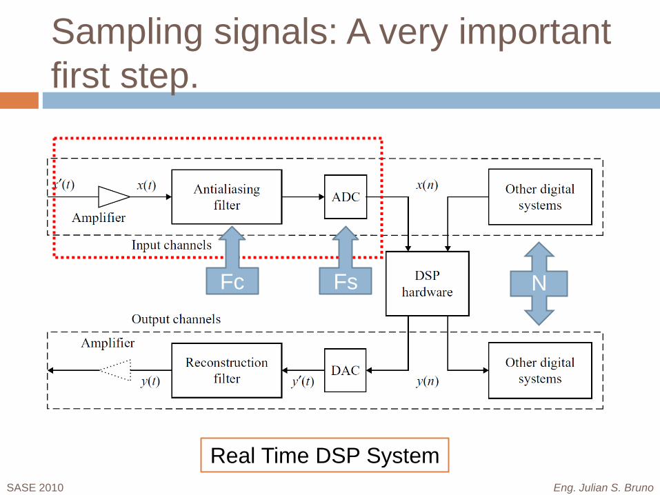
Sampling signals: A very important first step.



Fc Fs N

Sampling low-pass signals (CT)


The sampling theorem indicates that a continuous signal can be properly sampled, only if it does not contain frequency components above one-half of the sampling rate.

NS ff 2≥Nyquist sampling theorem

Aliasing and frequency ambiguity


Sampling band-pass signals


for any positive integer m, where fs ≥ 2B is accomplished.1

22++

≥≥−

mBff

mBf c

sc

IF samplingHarmonic

samplingSub-Nyquist

samplingUndersampling

Sampling band-pass signals

m (2Fc-B)/m (2Fc-B)/(m+1) Optimum Fs

1 35.0 MHz 22.5 MHz 22.5 MHz

2 17.5 MHz 15.0 MHz 17.5 MHz

3 11.66 MHz 11.25 MHz 11.25 MHz

4 8.75 MHz 9.0 MHz -

5 7.0 MHz 7.5 MHz -


Reconstruction signals



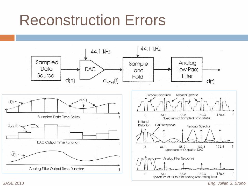
Reconstruction Errors


DSP hardware



What can we do with a DSP?


Almost any linear and nonlinear system (PID controller).

Digital filters (FIR-IIR). Adaptive systems (LMS algorithm). Modulators and demodulators. Any mathematical intensive algorithm (FFT-

DCT-WT).

Real time constraints


Algorithms time (tA) MUST fit between two consecutive sampling periods (tS).

Thus tA limits the maximum frequency that a system can work.

The definition of real time is VERY application dependant (faster speed of evolution of the system).

Linear systems implementation


Being x(n) and h(n) are arrays of numbers. If we want to compute y(n) we have to multiply and sum the last M samples, being M the length of h(n). This repeated for every new sample received from de ADC.

As you can see, any linear system uses multiplications, accumulations (sums), and loops intensively.

Fast Fourier Transform FFT


Summary of desirable features of a DSP


Fast in mathematics operations, and combinations of them (multiply and sum specially).

Flexible addressing modes (bit reversal, circular buffers, zero overhead loops)

DSP specific instruction set (arithmetic shifting, saturating arithmetic, rounding, normalization)

Minimum overhead peripherals (communications devices specially)

Application specific DSP instructions (Video, Control, Audio)

So, those are DSP math features


Multiply and Accumulators (MAC’s) units.

ALU’s (fixed and floating point).

Barrel shifters. Depending on DSP

application, more than one unit are present in modern DSP’s, allowing parallelism.

Harvard (modified) architecture provide multiple operations per cycle.

Another important features


RISC like registers and instruction set

Multiple data/program buses.

Address generator units for flexible addressing and efficient looping.

DMA controller for handling peripherals.

DSP clasification


Fixed or Floating point arithmetic. Millions of multiply–accumulate operations per

second, MMACs. Millions of floating-point operations per

second, MFLOPS. Application specific features (video, audio,

control, communications). Memory

Why DSP hardware?


Special-purpose (custom) chips such as application-specific integrated circuits (ASIC).

Field-programmable gate arrays (FPGA). General-purpose microprocessors or microcontrollers (μP/μC). General-purpose digital signal processors (DSP processors). DSP processors with application-specific hardware (HW)

accelerators.

ADI Processors


TigerSHARC® Processors 32-bit fixed-point as well as floating-point Clock Speed: 250MHz to 600MHz 4.8 GMACs of 16-bit performance / 3.6 GFLOPs 24 Mbits of on- chip memory 5 Gbytes of I/O bandwidth

SHARC® Processors 32-Bit floating-point Clock Speed: 150MHz to 400MHz / 2.4 GFLOPs. Accelerator Architecture: FIR, IIR, FFT.

Blackfin® Processors 16/32-bit fixed point Clock Speed: 200MHz to 756MHz / 1.5 GMACs Very low power consumption: 0.23mW/Mhz RTOS supported. Multicore 600MHz / 2.4 GMACs.

ADSP-21xx Processors 16/32-bit fixed point Clock Speed: 75MHz to 160MHz Analog Devices brought first programmable processor to market in 1986

Blackfin ProcessorsADSP-BF536/ADSP-BF537 BLOCK DIAGRAM


Some important operations

Quad 16-Bit OperationsR3 = R0 +|+ R1, R2 = R0 –|– R1 (S) ;

Dual 32-Bit OperationsR3 = R1 + R2, R4 = R1 – R2 (NS) ;

R3 = A0 + A1, R4 = A0 – A1 (S) ;

Dual MAC OperationsA1 += R1.H * R2.L, A0 += R1.L * R2.H;R3.H = (A1 += R1.H * R2.L), R3.L = (A0 += R1.L * R2.L);


Code Examples

FIRP4 = length(kernel)-1;Limpio el acumulador y tomo las muestras para la primera suma, multiplicación y acumulación

A0 = 0 || W[I1--] = R0.L || R1.H = W[I0++];LSETUP ( loop , loop ) LC1 = P4;

loop : A0 += R0.L * R1.H || R0.L = W[I1--] || R1.H = W[I0++];Hago la ultima multiplicación, y guardar el resultado

R0 = (A0 += R0.L * R1.H);


Markets and Applications


Recommended bibliography

UTN-FRBA 2010 Eng. Julian S. Bruno

RG Lyons, Understanding Digital Signal Processing 2nd ed. Prentice Hall 2004. Ch2: Periodic Sampling

SW Smith, The Scientist and Engineer’s guide to DSP. California Tech. Pub. 1997. Ch1: The Breadth and Depth of DSP Ch3: ADC and DAC

SM Kuo, BH Lee. Real-Time Digital Signal Processing 2nd ed. John Wiley and Sons. 2006 Ch1:Introduction to Real-Time Digital Signal Processing

NOTE: Many images used in this presentation were extracted from the recommended bibliography.

Thank you!

Questions?

SASE 2010Eng. Julian S. Bruno

real time igital signal...

Documents