Bachelor-Thesis

Real Time Image Distortion for Manual Image

Alignment

Georg Marius

Matr.Nr: 0130194

mariusg@sbox.tugraz.at

Technical University Graz

2010

2

AbstractIn the last years the digitalisation of image capturing, processing and display was one of the fastest growing fields on

the technological market.

With this new quality and quantity of digital images and the rising computational power the field of image

registration has become more and more popular.

The field of image registration reaches from medical uses (e.g. aligning computer tomography images) over new

mapping and environment viewing services like Google maps or Google street view, to processing images for

panorama- or high dynamic range (HDR) - image creation.

The latter is also the main motivation for this thesis which takes a look into the usage of different image distortion

methods for the case of manual image alignment.

3

Abstract ................................................................................................................................................2

Introduction..........................................................................................................................................4

Motivation........................................................................................................................................4

Related work ........................................................................................................................................5

Algorithms ...........................................................................................................................................6

Lens distortion..................................................................................................................................6

Pre alignment ...................................................................................................................................8

Beier Neely ......................................................................................................................................9

Moving least squares......................................................................................................................12

Energy minimisation ......................................................................................................................20

Grid smoothing using cubic spline interpolation ...........................................................................21

Shaders ...........................................................................................................................................25

Interface creation................................................................................................................................26

The environment ............................................................................................................................26

Processing and displaying images..................................................................................................26

Save, load and export .....................................................................................................................27

Work flow ......................................................................................................................................27

Results................................................................................................................................................28

Performance results:.......................................................................................................................28

Performance tables:........................................................................................................................29

Real world examples......................................................................................................................30

Future work ........................................................................................................................................33

Literature:...........................................................................................................................................33

List of tables.......................................................................................................................................36

List of figures .....................................................................................................................................36

4

IntroductionMotivation

The motivation for this bachelor thesis is to create a program that allows an easy manual alignment of photos as pre-

processing step for the creation of panorama- and HDR-images (with the main focus on HDR- images).

When it comes to image alignment two basic approaches dominate the state of the art.

• “One approach is to shift or warp the images relative to each other and to look at how much the pixels

agree. Approaches that use pixel-to-pixel matching are often called direct methods.” [Stitching Tutorial, 06]

• “The other major approach is to first extract distinctive features from each image, to match these features to

establish a global correspondence, and to then estimate the geometric transformation between the images.”

[Stitching Tutorial, 06]

“Feature-based algorithms are commonly faster and more robust against scene movement or changes in general

scene luminosity than algorithms that only focus on pixels dissimilarities and therefore are part of most common

image stitching tools.” [Stitching Tutorial, 06]

Many popular programs for automatic or semi automatic image alignment use feature-based algorithms and

automated feature detection to reduce the effort for the user.

“One of the most popular algorithms used in feature recognition is David Lowe’s Scale Invariant Feature Transform

(SIFT) algorithm. [Lowe, D. G. (2004).].” [Stitching Tutorial, 06]

But in some cases, especially when the images to be matched have highly different exposures (as it is often the case

with images used in HDR photography), automated feature detection algorithms reach their limits and manual

interventions turns out to be helpful.

The focus of this thesis is on three issues:

• Manual user control: The idea is to give the user full control over the distortions. Because controlling the

position of each pixel is far from comfort all algorithms in this thesis build on feature based image

registration methods. But to allow full manual control the extraction of the source and destination positions

of the features, that serve has handles for image deformation, is not done by one of the common methods

(e.g. SIFT) but lies in hands of the user who can set these values by mouse.

• Usability: the application should provide an intuitive an ergonomic user interface.

• Speed: But the major challenge, and the main distinction form existing applications, should be the demand

for, not just simple and fast handling but also, real time feedback for every action the user makes.

To further enhance the quality of the results it is often a good idea to pre-process images to compensate effects like

lens distortion, rotations and translations (from making hand-held pictures) or scale differences.

5

Related workTo provide optimal preconditions for the actual distortion algorithms the images first go through the process of

correcting lens distortions and pre alignment.

Lens distortion/correction:

When talking about lens distortion one usually refers to the radial distortion that causes the image to look bowled out

(barrel distortion) or bowled in (pincushion distortion). This effect often occurs when using wide angle or tele lenses.

To compensate for these effects algorithms usually use low-order polynoms to recompute the positions for each pixel

based on its distance to the image. This and more complex lens correction algorithm where described by Brown in

1971 [Brown] and Slama in 1980 [Slama] [Stitching Tutorial, 06].

Pre-alignment:

There a several methods to create a good global alignment. Certainly worth mentioning is this context is the 8-point

algorithm described by H.C. Longuet-Higgins [8-point H.C. Longuet-Higgins] and the improved version of this

algorithm by Richard I. Hartley [8-point+ Richard I. Hartley] to create a projective matrix that applied to the image

creates the best global alignment for all feature points. Other methods are described in [Haitao et al.], [Agarwal et

al.] and [Zang et al].

But for this project with the speed requirement in mind a far less complex algorithm was chosen that simply

calculates the average scale, rotation and the translation for the image based on the vectors between the feature points

in their source and destination position.

For the actual image distortion three different approaches where implemented.

1. Beier Neely: The so called “field morphing” [Beier Neely] approach by Thaddeus Beier and Shawn Neely

describes a feature base method to transform one image into another based on a “field of influence”

surrounding specified control handles. The goal was to create a more realistic alternative for previous

existing 2D morphing techniques to simulate the transformation of one person or creature into another in the

context of video animation. A famous example for the application of this method is the Michael Jackson

music video “Black or White”.

2. Moving least squares: The approach for “image deformation using moving least squares” was presented by

[Schaefer et al.] and has its aim on deforming images in a “natural” and intuitive fashion. It builds mainly

on the work of [Igarashi et al.] and the idea of “as rigid as possible” image deformation (first described by

[Alexa et al.]) that states that a transformation looks the most natural when global and local deformations

avoid superfluous scaling or shearing. To steer deformation this approach, like the Beier Neely method, uses

a set of (user defined) features as control handles. The main idea is to create a distortion for an image by

giving every point in the image its own affine transformation matrix using “moving least squares” [Levin

1998]. Meaning that the least squares approximation for the 2*2 transformation matrix is solved based on

the source and destination positions of the control handles where the handles influences are weighted based

on the distance to the point that is evaluated. The name “moving least squares” yields from the fact that the

solution for the least square problem is dependent on the point of evaluation. To generate the most intuitive

and “natural” deformations the focus of the work by [Schaefer et al.] lies on restricted subclasses of affine

deformations, specifically on similarity and rigid transformations.

3. Energy minimisation: The approach of finding a deformation for a image through energy minimisation is a

grid based method driven by the idea that a deformed image should look the most natural when local

deformations are minimal i.e. neighbouring grid cells should look as similar as possible.

6

To find such a distortion a gradient descent minimization is done for an energy function in which variations between

neighbouring edges, changes of angles and the distance from the current position of the control handles to their

destination raise the overall energy.

Grid smoothing using cubic spline interpolation:

With the exception of the energy minimization approach, all of the mentioned transformation and deformation

methods could be performed at pixel resolution level and do not require a triangulation or rasterising. However since

pixel resolution computation is usually very time consuming and with the speed requirement in mind, images in this

project are split into a grid mesh with user defined dimensions, allowing the user to choose the relation of speed to

precision.

To compensate visible edges with low grid resolutions (which might be chosen for speed enhancement), a higher

resolution grid is created after deformation processing in which in between values of the original grid are computed

using cubic spline interpolation.

Shader:

To assist the user in finding corresponding features, functions like transparency regulation, colour inversion and an

edge detector using “Sobel convolutions”[Sobel], to highlight features even in regions with low contrast, were

implemented as fragment shaders, using the OpenGL shader language GLSL, making direct use of the GPU parallel

processing strength.

AlgorithmsLens distortion

“The radial distortion model says that coordinates in the observed images are displaced away (barrel distortion) or

towards (pincushion distortion) the image centre by an amount proportional to their radial distance.” [Stitching

Tutorial, 06]

Image 1: Barrel distortion and Pincushion distortion.

Distortion effects like this are especially a problem when aligning panoramas where overlapping parts are usually in

the outer regions of the image where the effects of lens distortions are the strongest. To compensate for these effects

the image is deformed by re-calculating the undistorted positions of the pixels. This is done by adjusting the length of

the vector from the image centre to each pixel by applying a low-order polynom.

7

Different sources suggest slightly different polynoms like:

( )( )4

42

2

44

22

1

1

rkrkyy

rkrkxx

++=′

++=′[Stitching Tutorial, 06] [Brown] [ Candocia]

or

( )( )4

43

32

2

44

33

22

1

1

rkrkrkyy

rkrkrkxx

+++=′

+++=′[PanoTools]

With radius 22 yxr += ,

y

xas the old,

′′

y

x as the new coordinates of the pixel with respect to the image

centre and 2k , 3k and 4k as radial distortion parameters.

The latter formula was chosen in this project.

To make this formula scale independent

y

x need to be the normalised versions of the actual pixel coordinates with

respect to the image dimension:

=

lengthnorm

ypixellengthnorm

xpixel

y

x

_

__

_

The reverse scaling is applied to retrieve pixel values:

′′

=

′′

lengthnormy

lengthnormx

ypixel

xpixel

_*

_*

_

_

where ( )heightwidthlengthnorm ,max_ = .

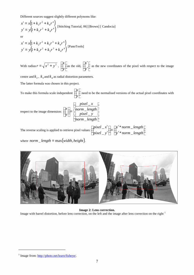
Image 2: Lens correction.Image with barrel distortion, before lens correction, on the left and the image after lens correction on the right 1

1 Image from: http://photo.net/learn/fisheye/.

8

Pre alignment

Image 3: Prealignment.

With the focus on HDR photography and the speed requirement in mind a rather simple pre-alignment approach was

chosen, that transforms the images only in terms of rotation uniform scaling and translation, instead of creating a

more precise but time costly perspective transformation (e.g. enhanced 8-point algorithm [8-point+ Richard I.

Hartley]).

The transformation is calculated based on the displacement of the user selected control handles and depends on the

number of handles.

Pre-alignment for one handle:

For one handle the whole image is translated directly using the handle translation.

( )00 hhvv ii −′+=′

with iv as source and iv′ as destination coordinates for each point in the image and 0h as source and 0h′ as destination

position of the handle.

Pre-alignment for two handles:

For two handles rotation, uniform scaling and translation can be applied.

( )00

0

0

010

010

, cvecvegetAngle

cve

cvescale

hhcve

hhcve

rr

r

r

r

r

′=

′=

′−′=′−=

α

where 1h and 1h′ are the source and destination position of the second handle, 0cver

and 0cver′ are the vector between

9

the first and the second handle in their source and destination position, scale as the scaling factor and α as the

angle between 0cver

and 0cver′

To get the translation vector the transformations for scale and rotation are applied on 0h

( ) ( )( ) ( ) scale

h

hh

y

x *cossin

sincos

0

00

−=

αααα&

And the translation vector is calculated as:

00 hht &r−′=

With the values for scaling, rotation and translation the formula for every point in the image is:

( ) ( )( ) ( ) tscale

v

vv

iy

ix

i

r+

−=′ *

cossin

sincos

αααα

Pre-alignment more than two handles:

For more than two handles average values for rotation and scale are computed.

( )∑

∑

′=

′=

′−′=′−=

i

ii

i

i

i

ii

ii

cvecvegetAnglei

cve

cve

iscale

hhcve

hhcve

0

0

0

0

,1

1

rr

r

r

r

r

α

The formula for translation is the same as for two handles, as is the computation of iv .

Though it is a quite rough approach it is usually sufficient for pre-alignment in this project, considering that the

images to be aligned will usually be taken for HDR creation and won’t have large distinctions in their perspective

which could cause problems since perspective transformations are not part of this pre-alignment algorithm.

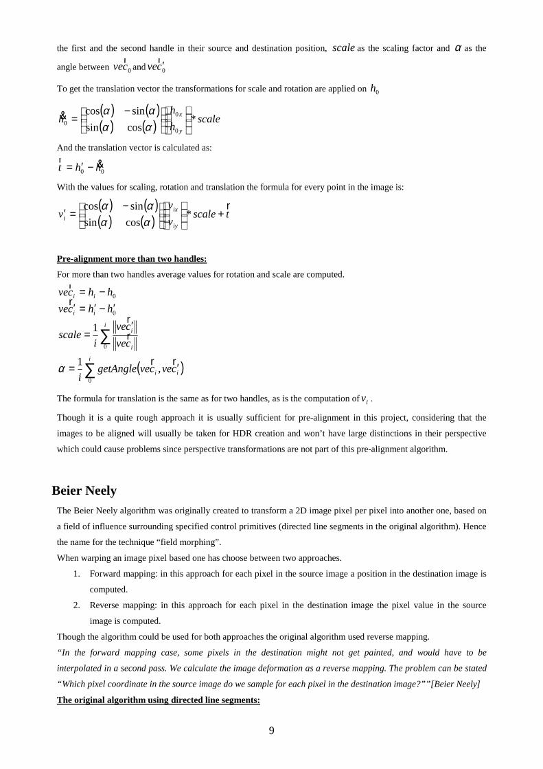
Beier Neely

The Beier Neely algorithm was originally created to transform a 2D image pixel per pixel into another one, based on

a field of influence surrounding specified control primitives (directed line segments in the original algorithm). Hence

the name for the technique “field morphing”.

When warping an image pixel based one has choose between two approaches.

1. Forward mapping: in this approach for each pixel in the source image a position in the destination image is

computed.

2. Reverse mapping: in this approach for each pixel in the destination image the pixel value in the source

image is computed.

Though the algorithm could be used for both approaches the original algorithm used reverse mapping.

“In the forward mapping case, some pixels in the destination might not get painted, and would have to be

interpolated in a second pass. We calculate the image deformation as a reverse mapping. The problem can be stated

“Which pixel coordinate in the source image do we sample for each pixel in the destination image?””[Beier Neely]

The original algorithm using directed line segments:

10

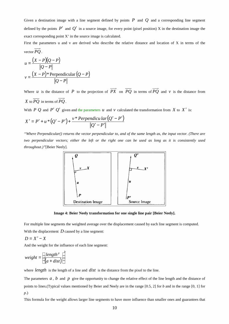
Given a destination image with a line segment defined by points P and Q and a corresponding line segment

defined by the points P′ and Q′ in a source image, for every point (pixel position) X in the destination image the

exact corresponding point X’ in the source image is calculated.

First the parameters u and v are derived who describe the relative distance and location of X in terms of the

vector PQ .

( )( )

( ) ( )PQ

PQPXv

PQ

PQPXu

−−−

=

−−−

=

lar Perpendicu*

Where u is the distance of P to the projection of PX on PQ in terms of PQ and v is the distance from

X to PQ in terms of PQ .

With P Q and P′ Q′ given and the parameters u and v calculated the transformation from X to X ′ is:

( ) ( )PQ

PQlarPerpendicuvPQuPX

′−′′−′

+′−′+′=′ **

“Where Perpendicular() returns the vector perpendicular to, and of the same length as, the input vector. (There are

two perpendicular vectors; either the left or the right one can be used as long as it is consistently used

throughout.)”[Beier Neely].

Image 4: Beier Neely transformation for one single line pair [Beier Neely].

For multiple line segments the weighted average over the displacement caused by each line segment is computed.

With the displacement D caused by a line segment:

XXD −′=And the weight for the influence of each line segment:

( )

bp

dista

lengthweight

+

=

where length is the length of a line and dist is the distance from the pixel to the line.

The parameters a , b and p give the opportunity to change the relative effect of the line length and the distance of

points to lines.(Typical values mentioned by Beier and Neely are in the range [0.5, 2] for b and in the range [0, 1] for

p.)

This formula for the weight allows larger line segments to have more influence than smaller ones and guarantees that

11

the influence of a line segment on a point becomes greater the closer the point is located to the line segment.

Image 5: Beier Neely transformation for multiple line pairs. [BeierNeely]

The adapted algorithm using directed line segments:

Since the algorithm for this project is meant to use points as handles instead of line segments, the algorithm was

slightly adjusted. The displacement for each point is now based only on the translation of the control handles and so

the calculation of the displacement D is simplified to:

PPD −′=

In the weight formula the parameters length and p that are related to the length of the line segment where

removed, yielding the adjusted formula for the weight of point handles:

( )

b

distaweight

+

=1

Although the change from line segments to points does not offer quite the variety of transformations possible with

line segments (e.g. stabilisation over long areas or local rotations that are possible with line segments are much

harder to create with points) but due to the simplifications it is faster and still generates sufficiently smooth

deformations.

Image 6: Beier Neely sample.Results of image deformation with different values for the parameters a and b : Left undistorted, middle 1=a and 1=b and

right 100=a and 7=b .

12

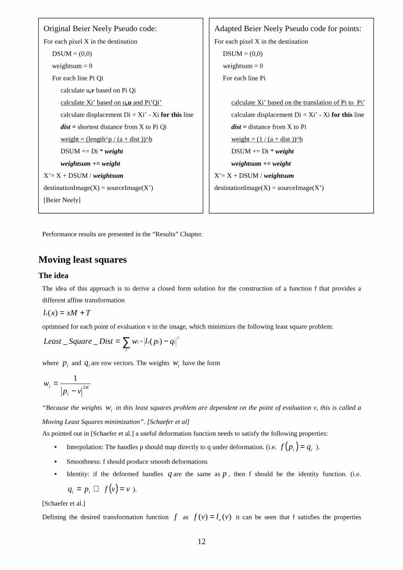
Performance results are presented in the “Results” Chapter.

Moving least squares

The idea

The idea of this approach is to derive a closed form solution for the construction of a function f that provides a

different affine transformation

TxMxlv +=)(

optimised for each point of evaluation v in the image, which minimizes the following least square problem:

∑ −=i

iivi qplwDistSquareLeast2

)(__ *

where ip and iq are row vectors. The weights iw have the form

α2

1

vpw

i

i−

=

“Because the weights iw in this least squares problem are dependent on the point of evaluation v, this is called a

Moving Least Squares minimization”. [Schaefer et al]

As pointed out in [Schaefer et al.] a useful deformation function needs to satisfy the following properties:

• Interpolation: The handles p should map directly to q under deformation. (i.e. ( ) ii qpf = ).

• Smoothness: f should produce smooth deformations

• Identity: if the deformed handles q are the same as p , then f should be the identity function. (i.e.

( ) vvfpq ii =⇒= ).

[Schaefer et al.]

Defining the desired transformation function f as )()( vlvf v= it can be seen that f satisfies the properties

Adapted Beier Neely Pseudo code for points:

For each pixel X in the destination

DSUM = (0,0)

weightsum = 0

For each line Pi

calculate Xi’ based on the translation of Pi to Pi’

calculate displacement Di = Xi’ - Xi for this line

dist = distance from X to Pi

weight = (1 / (a + dist ))^b

DSUM += Di * weight

weightsum += weight

X’= X + DSUM / weightsum

destinationImage(X) = sourceImage(X’)

Original Beier Neely Pseudo code:

For each pixel X in the destination

DSUM = (0,0)

weightsum = 0

For each line Pi Qi

calculate u,v based on Pi Qi

calculate Xi’ based on u,u and Pi’Qi’

calculate displacement Di = Xi’ - Xi for this line

dist = shortest distance from X to Pi Qi

weight = (length^p / (a + dist ))^b

DSUM += Di * weight

weightsum += weight

X’= X + DSUM / weightsum

destinationImage(X) = sourceImage(X’)

[Beier Neely]

13

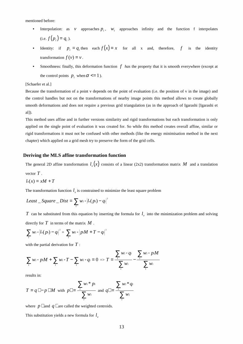
mentioned before:

• Interpolation: as v approaches ip , iw approaches infinity and the function f interpolates

(i.e. ( ) ii qpf = ).

• Identity: if ii qp = then each ( ) xxf = for all x and, therefore, f is the identity

transformation vvf =)( .

• Smoothness: finally, this deformation function f has the property that it is smooth everywhere (except at

the control points ip when 1<=α ).

[Schaefer et al.]

Because the transformation of a point v depends on the point of evaluation (i.e. the position of v in the image) and

the control handles but not on the transformations of nearby image points this method allows to create globally

smooth deformations and does not require a previous grid triangulation (as in the approach of Igarashi [Igarashi et

al]).

This method uses affine and in further versions similarity and rigid transformations but each transformation is only

applied on the single point of evaluation it was created for. So while this method creates overall affine, similar or

rigid transformations it must not be confused with other methods (like the energy minimisation method in the next

chapter) which applied on a grid mesh try to preserve the form of the grid cells.

Deriving the MLS affine transformation function

The general 2D affine transformation ( )xlv consists of a linear (2x2) transformation matrix M and a translation

vector T .

TxMxlv +=)(

The transformation function vl is constrained to minimize the least square problem

∑ −=i

iivi qplwDistSquareLeast2

)(__ *

T can be substituted from this equation by inserting the formula for vl into the minimization problem and solving

directly for T in terms of the matrix M .

∑ −i

iivi qplw2

)(* = ∑ −+i

iii qTMpw2

*

with the partial derivation for T :

0*** =−+ ∑∑∑i

ii

i

i

i

ii qwTwMpw => ∑

∑∑

∑−=

i

i

i

ii

i

i

i

ii

w

Mpw

w

qwT

**

results in:

MpqT ∗−∗= with∑

∑=∗

i

i

i

ii

w

pwp

* and

∑∑

=∗

i

i

i

ii

w

qwq

*

where ∗p and ∗q are called the weighted centroids.

This substitution yields a new formula for vl

14

∗+∗−= qMpxxlv )()(

and allows rewriting the least squares problem in the form:

∑ −=i

iii qMpwceDisSquareLeast2

ˆˆtan__ *

where ∗−= ppp iiˆ and ∗−= qqq iiˆ .

The transformation matrices for each point can now be calculated by solving the least squares problem using the

normal equations solution:

∑∑−

=

jj

Tjj

iii

Tiaffine qpwpwpM ˆˆˆˆ

1

“Though this solution requires the inversion of a matrix, the matrix is a constant size (2*2) and is fast to invert.”

[Schaefer et al.]

With the least square approximation for affineM the complete formula for )(vf affine is:

∗+∗−= qMpvvf affineaffine )()(

∗+

∗−= ∑∑

−

qqpwpwppvvfj

jTjj

iii

Tiaffine ˆˆˆˆ)()(

1

The results of the transformation on the image and a representation of the transformation matrices for each point can

be seen in the following figure

Image 7: MLS affine transformation.The green circles in the left image are the positions of p while the green circles in the right image are the positions of

q. Red lines show the raster of the image mesh. Blue circles show the positions of v in the image on the left and of

)(vf affine on the right. The blue quads show the affine transformation that was applied to this particular point v in

the image.

Using this MLS affine transformation function leads to quite satisfying (expected) distortions under the condition

15

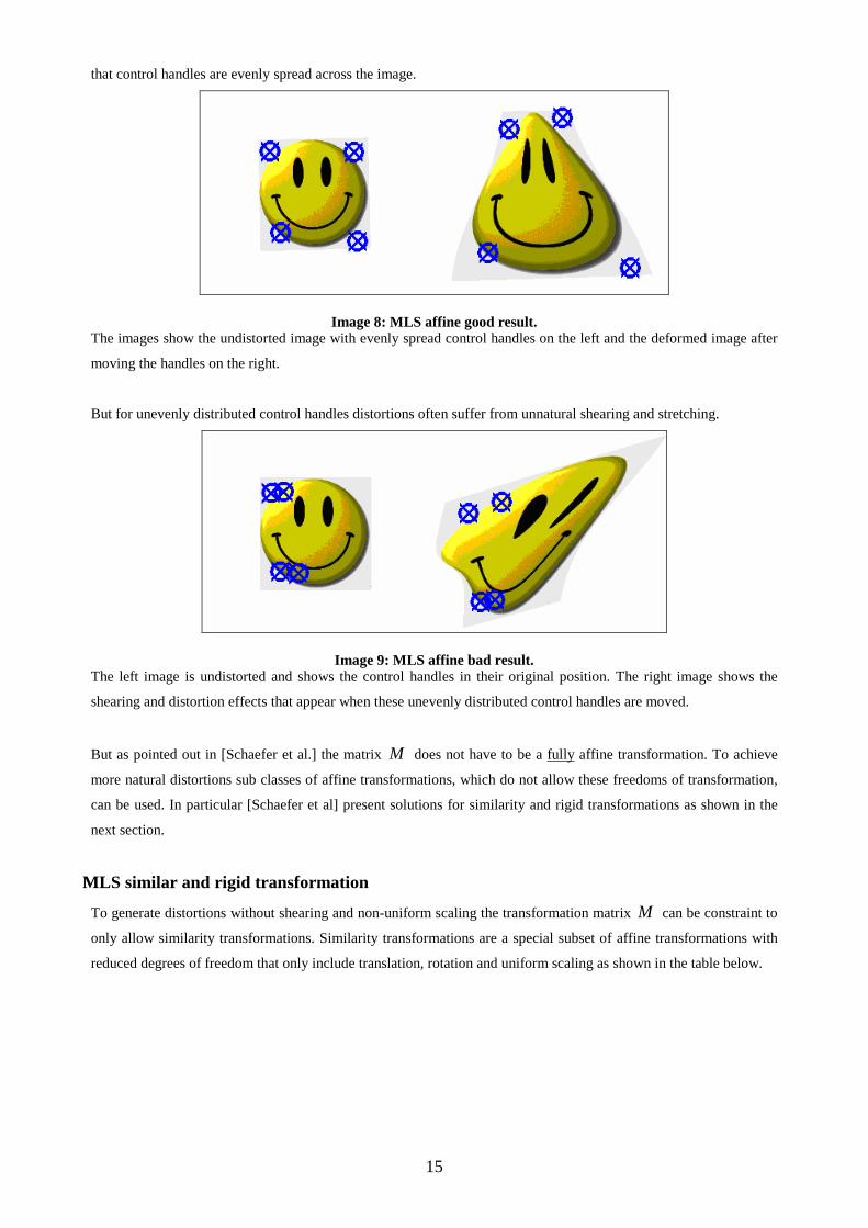
that control handles are evenly spread across the image.

Image 8: MLS affine good result.The images show the undistorted image with evenly spread control handles on the left and the deformed image after

moving the handles on the right.

But for unevenly distributed control handles distortions often suffer from unnatural shearing and stretching.

Image 9: MLS affine bad result.The left image is undistorted and shows the control handles in their original position. The right image shows the

shearing and distortion effects that appear when these unevenly distributed control handles are moved.

But as pointed out in [Schaefer et al.] the matrix M does not have to be a fully affine transformation. To achieve

more natural distortions sub classes of affine transformations, which do not allow these freedoms of transformation,

can be used. In particular [Schaefer et al] present solutions for similarity and rigid transformations as shown in the

next section.

MLS similar and rigid transformation

To generate distortions without shearing and non-uniform scaling the transformation matrix M can be constraint to

only allow similarity transformations. Similarity transformations are a special subset of affine transformations with

reduced degrees of freedom that only include translation, rotation and uniform scaling as shown in the table below.

16

Image 10: Hierarchy of 2D transformations.

“The 2x3 matrices are extended with a third [ ]10T row to form a full 3x3 matrix for homogeneous

transformations.” [Stitching Tutorial, 06]

Similarity transformation:

To restrict M to only allow similarity functions it has to satisfy the additional property: IMM T 2λ= .

If M is a block matrix of the form

( )21 MMM =

where 1M , 2M are column vectors of length 2, then restricting M to be a similarity transform requires that

22211 λ== MMMM TT and 021 =MM T . This constraint implies that ⊥= 12 MM where

applied on a vector, returns a perpendicular vector of the same length e.g. ( ) ( )xyyx −=⊥.

[Schaefer et al.]

With this the minimization problem can be written as:

∑ −

−

= ⊥i

Ti

i

ii qM

p

pwDistSquareLeast

2

ˆˆ

ˆ__ 1*

Changing the formula for M to:

( )Ti

Ti

i

i

ii

similarsimilar qq

p

pM ⊥

⊥ −

−

= ∑ ˆˆˆ

ˆ1ω

µ

with Tii

iisimilar pp ˆˆ∑= ωµ

With the solution for similarM the final formula for )(vf similar is:

∗+∗−= qMpvvf similarsimilar )()(

( ) ∗+−

−

∗−= ⊥⊥∑ qqq

p

ppvvf T

iTi

i

i

ii

similarsimilar ˆˆ

ˆ

ˆ1)()( ω

µ

17

Rigid transformation:

To further restrict M to only allow rigid transformations [Schaefer et al] provides a theorem which explains how

rigid transformations are related to the similarity transformations.

Theorem :

Let C be the matrix that minimizes the following similarity functional:

∑ −= i

iiiIMM

qMpwT

2ˆˆmin

2λ

If C is written in the form Rλ where R is a rotation matrix and λ is

a scalar, the rotation matrix R minimizes the rigid functional

∑ −= i

iiiIMM

qMpwT

2ˆˆmin

[Schaefer et al.]

With that theorem the only change to the computation of similarM is in the term µ :

22

ˆˆˆˆ

+

= ∑∑ ⊥

i

Tiii

i

Tiiirigid pqpq ωωµ

( )Ti

Ti

i

i

ii

rigidrigid qq

p

pM ⊥

⊥ −

−

= ∑ ˆˆˆ

ˆ1 ωµ

yielding the final formula for )(vf rigid :

∗+∗−= qMpvvf rigidrigid )()(

( ) ∗+−

−

∗−= ⊥⊥∑ qqq

p

ppvvf T

iTi

i

i

ii

rigidrigid ˆˆ

ˆ

ˆ1)()( ω

µ

To speed up deformation calculations the formulas for affine, similarity and rigid transformations can be further

rephrased to allow pre-computation for major parts of the processing in order to achieve faster deformations for

constant values of v and p , as described in the next section.

MLS Speedup through Pre-computation

Manual manipulation of the image by the user happens by selecting a handle’s source position by clicking on a point

in the image and dragging it to its destination position.

During the drag and until a new handle is added, the values for v and p stay the same and only the values for q

change. This observation leads to the idea of pre-computing parts of the transformation that do not involve q .

Due to the different involvement of q in the formulas there is a variation in which parts can be pre-computed

between affine, similarity and rigid transformations.

Affine pre-computation:

The formula for affinef can be rephrased to:

∗+= ∑ qqAvfj

jjaffine ˆ)(

Where jA is a single scalar, which can be pre-computed, given as:

18

( ) Tj

iii

Tij ppwppvA ˆˆˆ

1−

∗−= ∑

Similarity pre-computation:

As with the unrestricted transformation the formula can be rewritten in a way that allows to pre-compute most of the

necessary processing.

∗+

= ∑ pAqf i

similari

isimilar µ

1ˆ

with ( )

T

i

ii pv

pv

p

pA

∗−−∗−

−

= ⊥⊥ˆ

ˆω

where A and similarµ can be pre computed.

Rigid pre-computation:

Because of the involvement of q in the calculation of rigidµ pre-computation for rigidfr

has to change to:

iii

rigid Aqvf ˆ)( ∑=r

∗+∗−= qvf

vfpvvf

rigid

rigidrigid

)(

)()( r

r

Due to the necessary normalization this transformation is not as efficient but still delivers a quite respectable

performance.

19

MLS comparison

To give a clear image of how results for the three versions of this method can vary this section provides some images

that visualise the distortions for each method.

Performance comparison and real world examples are provided in the “Results” chapter.

Transformation results:

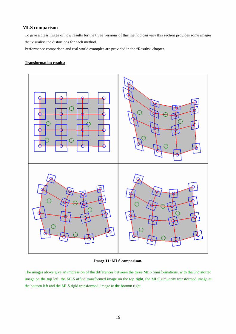
Image 11: MLS comparison.

The images above give an impression of the differences between the three MLS transformations, with the undistorted

image on the top left, the MLS affine transformed image on the top right, the MLS similarity transformed image at

the bottom left and the MLS rigid transformed image at the bottom right.

20

Energy minimisation

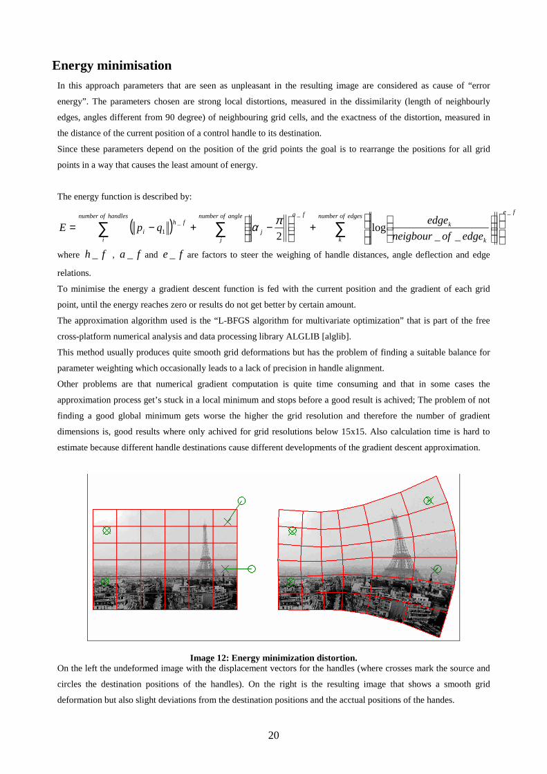
In this approach parameters that are seen as unpleasant in the resulting image are considered as cause of “error

energy”. The parameters chosen are strong local distortions, measured in the dissimilarity (length of neighbourly

edges, angles different from 90 degree) of neighbouring grid cells, and the exactness of the distortion, measured in

the distance of the current position of a control handle to its destination.

Since these parameters depend on the position of the grid points the goal is to rearrange the positions for all grid

points in a way that causes the least amount of energy.

The energy function is described by:

( )fe

edgesofnumber

k k

kangleofnumber

j

fa

j

handlesofnumber

i

fh

i edgeofneigbour

edgeqpE

___

1 __log

2 ∑∑∑

+

−+−=

πα

where fh _ , fa _ and fe _ are factors to steer the weighing of handle distances, angle deflection and edge

relations.

To minimise the energy a gradient descent function is fed with the current position and the gradient of each grid

point, until the energy reaches zero or results do not get better by certain amount.

The approximation algorithm used is the “L-BFGS algorithm for multivariate optimization” that is part of the free

cross-platform numerical analysis and data processing library ALGLIB [alglib].

This method usually produces quite smooth grid deformations but has the problem of finding a suitable balance for

parameter weighting which occasionally leads to a lack of precision in handle alignment.

Other problems are that numerical gradient computation is quite time consuming and that in some cases the

approximation process get’s stuck in a local minimum and stops before a good result is achived; The problem of not

finding a good global minimum gets worse the higher the grid resolution and therefore the number of gradient

dimensions is, good results where only achived for grid resolutions below 15x15. Also calculation time is hard to

estimate because different handle destinations cause different developments of the gradient descent approximation.

Image 12: Energy minimization distortion.On the left the undeformed image with the displacement vectors for the handles (where crosses mark the source and

circles the destination positions of the handles). On the right is the resulting image that shows a smooth grid

deformation but also slight deviations from the destination positions and the acctual positions of the handes.

21

Grid smoothing using cubic spline interpolation

Because pixel resolution processing of images would cost far too much computation time to allow real time

interaction, images are divided into a grid mesh with reduced resolution. In most cases a grid resolution between

20x20 and 50x50, depending on the image size, is sufficient to let distorted images look smooth.

But with very large images or a lower grid resolution sharp bends between edges of the grid become visible if

deformations are too strong. In addition deformations caused by OpenGL internally breaking up each quad of the

grid mesh into two independently linearly interpolated triangles can become visible, as shown in the figure below.

Image 13: Low resolution grid problems.The undistorted image with 3x3 grid resolution on the left. The distorted image on the right with clearly visible sharp

bends along the grid edges (red lines) and the distortion effect, caused by the internal break up of a quad into two

triangles, visible in the upper right quad, causing a sharp bend in the round outline of the smiley.

To suppress these effects without increasing the grid resolution for distortion calculations a grid smoothing algorithm

using cubic spline interpolation is applied.

This method takes the distorted low resolution grid, iteratively generates cubic splines along the rows and columns

and creates a new high resolution grid using the interpolated values of the spline functions.

A cubic spline is defined piecewise by cubic functions between the values of the reference axis.

22

1D Spline

0

1

2

3

4

5

6

7

0 1 2 3 4 5 6 7 8 9 10

X

Y

lines

spline

piece 1

piece 2

piece 2

piece 4

Image 14: 1D cubic spline.The graphic shows the construction of a 1D spline with the point that describes the function. The cubic function that

describes the piecewise intervals between points are drawn in yellow, blue, purple an dark red in that order of the

pieces from left to right. The final spline is drawn as a thick red line.

To create a spline curve in a higher dimensional space (2D in this case) a separate spline curve for each of the space

axes has to be created for the same reference axis. In the case of 2D grid smoothing for each row and column of the

grid a spline for the X and Y coordinates of the row (or column) is created with the point indices as values for the

reference axis.

X - Y

0

5

10

15

20

25

30

0 5 10 15 20

X

Y

Image 15: Function points in 2D space.The given points of a curve in 2D space.

23

Image 16: Splitting a spline curve for 2D space.The left image shows a spline created from the X values with the row (column) index as reference axis. The right

image shows a spline created from the Y values with the row (column) index as reference axis.

X - Y

0

5

10

15

20

25

30

0,00 5,00 10,00 15,00 20,00

X

Y

Image 17: 2D spline curve.This picture shows the final spline curve in 2d space combined from the X and Y values of the two 1D splines in the

graphics above.

The particular type of spline used in this project is the so called ”Akima spline”. It is more robust against oscillation

in the neighbourhood of outliers compared to normal cubic splines, as the following graphic shows.

Image 18: Akima spline.The graphic [alglib] shows the comparison between a standard cubic spline (red line) and an Akima spline(green

24

line) in the neigbourhood of an outlier. As can be seen the standard cubic spline funktions shows some oscillation in

the neigbourhood of the outlier (fourth point from left) while the Akima spline function does not.

Below is a practical example for the usefulness of this grid smoothing method.

Image 19: Lens correction with low resolution grid.An image with a 5x5 grid resolution and a distortion due to lens correction. The sharp bends and the distortions of

internal quad triangulation are clearly visible on the outlines and the two buildings on the right.

Image 20: Lens correction with low resolution grid and spline interpolation.The same image as above were the 5x5 grid was interpolated with the grid smoothing technique described to get a

15x15 grid resolution.

Image 21: Lens correction with high resolution grid.The same image as the first one but with an initial 15x15 grid resolution.

25

Because spline interpolation of a grid is usually much faster than distortion calculations for a higher resolution grid

this method is especially useful for computationally intense methods like the energy minimisation method mentioned

before.

Performance results are presented in the “Results” chapter.

Shaders

To make alignment easier some functionality, to adjust and enhance images visibility properties, was implemented in

the form of OpenGL fragment shaders using the OpenGL shader language GLSL. That way the CPU is relieved of

intense pixel colour computation by using the parallel processing abilities of the GPU.

Transparency regulation: By setting a value on a scrollbar and sending it to the shader the amount of transparency for

an image can be set, making it easier to find the location of corresponding features in image layers below.

Magic lens: The magic lens is a feature that allows seeing through to the image layer selected in an area around the

mouse courser even if image layers above are not set to be transparent. To achieve that the selected image layer is

drawn a second time above all others, but this time the shader draws the layer completely transparent except for the

region around the mouse cursor coordinates, that where given to the shader.

Edge detection: To highlight edges, that are usually helpful to determine feature points, an edge detector [Mike

Bailey] using “Sobel convolutions” [Sobel] was implemented.

Colour inversion: This operation inverts the colour of each pixel generating a negative image. This turns out to be

highly useful in combination with the transparency and edge detection, because overlapping regions cancel each

other out when the original pixel values correspond, while non corresponding regions become more recognisable.

Image 22: Samples for transparency, magic lens and edge detection & inversion.

Image 23: Sample for function combination.Image 21 shows the aligning process with edge detection and colour inversion on the left and the result with both

images set to half transparent.

26

Interface creationThe environment

One of the main concerns was that the application should have an ergonomic graphical user interface. The

construction of such a user interface can be quite a challenge and since Microsoft’s Windows Forms package for C#

is a very comfortable tool to create graphical user interfaces the choice of the implementation language fell on C#.

Even with this support the major challenge, and the main distinction form existing applications, was the demand for

simple and fast handling as well as real time feedback for every user action.

Processing and displaying images

There a quite a few ways to hold, process and display images in a computer program.

Windows Forms package for C# has its own image format and the ”PictureBox” class that makes displaying of

images really easy, but working with these classes has the great disadvantage of having to do all calculations on the

CPU. First attempts quickly revealed that this approach would not satisfy the desired speed requirements.

The next approach was to use the parallel processing abilities of the GPU by turning the image into a texture and

performing all transformation operations in a fragment shader written in OpenGL Shading language (GLSL). First

tests with similarity transformations, transparency, colour inversion and edge highlighting seemed promising, but it

turned out that the gain of computation power is offset by the drawbacks of this approach.

Drawbacks:

• Render time increases not just with window size but also with the complexity of the deformation algorithm:

increased render time for larger display windows is normal. But when for each pixel (on the screen) that

should get its value from a certain texture, a deformation calculation (usually dependent on the number of

control handles) has to be made, rendering time increases by that factor.

• Limited use of libraries: Since most of the transformation calculation is done on the GPU the use of

external libraries is limited to the few pre-calculations done on the CPU. All algorithms used on the GPU

need to be re-implemented in the shading language.

• Costly backwards computation: To reduce time for deformation calculations the idea came up to divide

the texture internally into a grid and provide smoothness through spline interpolation. But no fast method to

compute the needed backwards computation of the texture coordinates for the fragment position was found.

In the end a combined approach was chosen. The image texture is partitioned into a grid mesh reducing the number

of points to be considered in distortion operations from the number of pixels in the image to the number of grid

points so the CPU processing speed is sufficient to do the calculations.

GPU support is now used for coordinate picking and display modes like transparency, colour inversion and edge

highlighting.

The drawback of potential rough edges when the grid dimension is insufficient for the degree of distortion can be

compensated by smoothing the grid, after it is distorted, using cubic spline interpolation, as described above.

27

Save, load and export

Since this application is used for image alignment but not for final merging of images a function to export all images

in their distorted and aligned state as “.png” or “.tiff” sequence was implemented. The size of the final image is

computed by the bounding box of all vertices in all image layers.

Also the whole project data, including the paths of the images, the source and destination positions of all control

handles and the distortion method for each image layer can be saved to an XML structured file. When opening such a

file the project is reconstructed from this information.

The same method is used to save user created lenses that are stored in a separate file and loaded during the

application start.

Work flow

The usual workflow for aligning images with this program consists of the following steps.

1. Loading the images: Images are loaded by using the menu entry “load Image” that provides a “File open

dialogue” and allows to select load multiple images for loading at the same time. New images can be loaded

at any time.

2. Lens settings and pre alignment: after loading images it makes sense to immediately apply the lens settings

to increase the precision for further alignment steps. If the correct lens settings are unknown the easiest way

to determine them is to align two images using only two handles (in this case handles should be set in both

images to lock image positions during lens calibration). Then select the same lens for both images and

calibrate it until the best alignment is achieved using the lens settings option from the “Extras” menu. Then

apply the lens to all images (assuming all images where taken with the same lens settings). After that the pre

alignment for all images can be done by selecting an image, creating a new handle by clicking on a point

and dragging it to its destination position. The use of shader functions like transparency control or the magic

lens can be helpful.

3. Distorting the images: after pre aligning the images a distortion method can be chosen for each image

individually. And exact alignment can be done by adding and placing further handles.

4. Save Project or export images: after alignment is done the hole project can be saved and the images can be

exported as image sequence in the “.png” or “.tiff” file format by using the corresponding menu entries that

provide a “File save dialogue”.

28

Image 24: Workflow.

Results This chapter describes the performance of the different algorithms and provides comparison tables and real world

examples for results (All table entries refer to computation on an Intel quad core processor with 2.4 GHz 3 GB RAM

and Windows Vista 32 bit version).

Performance results:

The performance for all implemented algorithms depends heavily on the number of vertices and the number of

control handles.

Beier Neely algorithm:

• A quite fast algorithm.

• Allows easy adaptation to different situations through freely choosable parameters.

• Produces good results (provided that the right parameter settings are chosen).

MLS algorithm:

• The overall fastest among the tested algorithms.

• Speedup through pre computation.

• Provides three variations where the “rigid” version usually gives the best results.

Energy minimization:

• The overall slowest of the tested algorithms.

• An Interesting approach but with some problems yet to be solved.

o Difficult to find the right weighting for the different parts of the energy function.

o Approximation gets often stuck in local minima resulting in bad results (especially for grid

resolutions larger than 15x15).

29

o Gradient calculation is very time consuming. (for now)

• Results provide smooth distortions but often lack in precision.

• Problems with grid resolutions larger than 15x15

Performance tables:

Pre-computation:

Pre-computation is only used with the MLS method and is usually only done when a control handle is added (or

removed) or the grid resolution is changed.

The following table shows the pre-computation times for all algorithms for different numbers of vertices and control

handles.

Distortion calculation:

The following table shows the performance for all algorithms (form MLS method after pre computation) for different

numbers of vertices and control handles.

Pre-

computation

time

(in ms)

vertices=20x20

handles=10

vertices=20x20

handles =20

vertices=50x50

handles =10

vertices=50x50

handles =20

vertices=100*100

handles =40

Beier Neely -------------- -------------- -------------- -------------- --------------

MLS Affine 8.46 11.5 25.44 44.0 311.76

MLS

Similar

8.96 12.88 29.26 53.46 375.94

MLS Rigid 8.62 11.66 26.28 46.28 324.28

Energy

minimizatio

n

-------------- -------------- -------------- -------------- --------------

Table 1: Performance table - Pre computation.

Computation

time (in ms)

vertices=20x20

handles=10

vertices=20x20

handles=20

vertices=50x50

handles=10

vertices=50x50

handles=20

vertices=100x100

handles=40

Beier Neely 8.16 18.96 46.32 119.94 5577.68

MLS Affine 0.165 1.0 4.64 8.22 68.48

MLS Similar 0.58 1.45 5.32 9.78 78.83

MLS Rigid 0.17 1.14 5.01 9.09 77.71

Energy

minimisation

15404.0 –

29090

early breaks

(bad result)

early breaks

(bad result)

early breaks

(bad result)

early breaks

(bad result)

early breaks

(bad result)

Table 2: Performance table - Computation.

30

Spline interpolation results:

Computation time ... (in ms) Beier Neely MLS rigid Energy minimisation

20x20 grid

10 handles

8.16 0.17 15404.0 - 29090

early breaks(bad result)

10x10 grid

+20x20spline smoothing

10 handles

1.69

+0.01

0.0(4269 Ticks)

+ 0.01

1844.0 – 6890.0

+ 0.01

50x50 grid

10 handles

46.32 5.01 early breaks(bad result)

10x10 grid

+50x50spline smoothing

10 handles

1.69

+1.08

0.0(4269 Ticks)

+1.08

1844.0 – 6890.0

+1.08

100x100 grid

20 handles

472.87 37.25 early breaks(bad result)

20x20 grid

+ 100x100 spline smoothing

20 handles

7.58

+4.29

1.46

+4.29

early breaks(bad result)

+4.29

Table 3: Performance table - Spline interpolation.

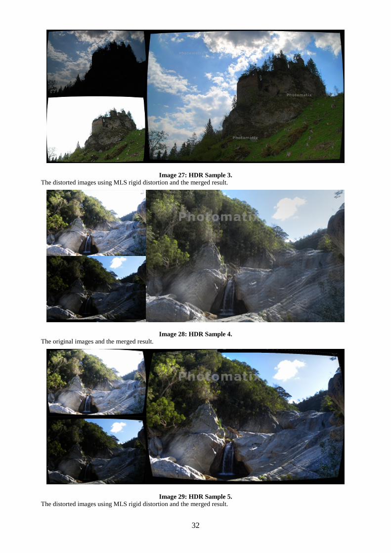
Real world examples

All examples where aligned a distorted with the application that was build as part of this thesis. The photos where

merged to HDR images using the “Photomatix” trial version.

31

Image 25: HDR Sample 1.The original images and the merged result can be seen on the left. The distorted images using MLS rigid distortion

and the merged result on the right.

Image 26: HDR Sample 2.The original images and the merged result.

32

Image 27: HDR Sample 3.The distorted images using MLS rigid distortion and the merged result.

Image 28: HDR Sample 4.The original images and the merged result.

Image 29: HDR Sample 5.The distorted images using MLS rigid distortion and the merged result.

33

Future workThere are quite a few ideas to further enhance the application.

Additional feature types: Additional types of control features (e.g. line segments) could be included to provide

more options for steering deformations.

Advanced rigid control: The MLS methods can be extended to consider special (user selected) regions that stay

more rigid. This can be done by adjusting the weights of the control handles for the vertices in the region with an

averaged weight over the region. This kind of extra rigidness can become useful when there are strong global

distortions where small regions (e.g. faces of people) should preserve their shape.

Speedup for Beier Neely algorithm: The Beier Neely method already provides a quite satisfying speed. But even

faster deformations would be possible by applying the concept of pre-computation, from the MLS algorithms, on the

weights for the Beier Neely algorithm. What has do be considered when implementing that change is that distortions

would look a little different than they do now because pre-alignment (that is now done on every point move event)

would not be done in order to use the pre-computed weights.

Auto fine tuning: A function similar to the automated fine tuning function of the Hugin tool could be implemented

to fine adjust handle positions using cross correlation. To overcome the problems of cross correlation for different

exposures the analysed parts of the image could be pre processed histogram equalization.

Auto snap function for easier feature placement: When selecting corresponding feature points in different images

an “auto snap” function similar to the one provided in the Pano Tools program [Pano Tools] could be implemented

by analysing the neighbourhood of the mouse courser for features corresponding to the selected point in the source

image, using a feature detection algorithms (e.g. SIFT . [Lowe, D. G. (2004). ]).

Literature:[Agarwal et al.]A Survey of Planar Homography Estimation Techniques

Anubhav Agarwal, C. V. Jawahar, and P. J. Narayanan

Centre for Visual Information Technology, International Institute of Information Technology

Hyderabad 500019 INDIA Email: pjn@iiit.ac.in

http://www.iiit.ac.in/techreports/2005_12.pdf

34

[Alexa et al.] As-Rigid-As-Possible Shape Interpolation – source

Marc Alexa: Darmstadt University of Technology

Daniel Cohen-Or: Tel Aviv University

David Levin: Tel Aviv University

http://citeseerx.ist.psu.edu/viewdoc/download?doi=10.1.1.21.3205&rep=rep1&type=pdf

[alglib] ALGLIB User Guide

http://www.alglib.net/interpolation/spline3.php#header0

[Beier Neely] Feature-Based Image Metamorphosis

Thaddeus Beier

Shawn Neely

http://www.cs.princeton.edu/courses/archive/fall00/cs426/papers/beier92.pdf

[Brown] Brown, D. C. (1971). Close-range camera calibration. Photogrammetric Engineering, 37(8),

855–866.

http://www.vision.caltech.edu/bouguetj/calib_doc/papers/Brown71.pdf

[ Candocia]A Scale-Preserving Lens Distortion Model and its

Application to Image Registration

Florida International University

Department of Electrical and Computer Engineering

10555 West Flager Street, EC-3915, Miami, FL. 33174, USA

(305)-348-3017

candocia@fiu.edu

http://www.eng.fiu.edu/mme/robotics/fcrar2006/papers/FCRAR2006-P18-Candocia-FIU.pdf

[Haitao et al.]A ROBUST ESTIMATION ALGORITHM OF EPIPOLAR GEOMETRY

THROUGH THE HOUGH TRANSFORM

Shan Haitao, Hao Xiangyangb, Wang Huia, Li Dawei, Li Jie

Middle Ring Road, Haidian District, Beijing 100088, P.R. China

Institute of Surveying and Mapping, Information Engineering University, 66 Longhai Road, Zhengzhou, 450052,

China

http://www.isprs.org/proceedings/XXXVII/congress/2_pdf/9_ThS-4/06.pdf

[Igarashi et al.] As-Rigid-As-Possible Shape Manipulation - rigid – source

Takeo Igarashi: The University of Tokyo

Tomer Moscovich: Brown University

John F. Hughes: PRESTO, JST

http://www-ui.is.s.u-tokyo.ac.jp/~takeo/papers/rigid.pdf

[LEVIN 1998 ]LEVIN, D. 1998. The approximation power of moving least squares.

35

Mathematics of Computation 67, 224, 1517–1531.

http://www.ams.org/mcom/1998-67-224/S0025-5718-98-00974-0/S0025-5718-98-00974-0.pdf

[Lombardi MLS matlab] Gabriele Lombardi

http://www.mathworks.com/matlabcentral/fileexchange/12249-moving-least-squares

[Lowe, D. G. (2004)]. Distinctive image features from scale-invariant keypoints. International

Journal of Computer Vision, 60(2), 91–110.

[Mike Bailey] Mike Bailey

Oregon State University

http://web.engr.oregonstate.edu/~mjb/cs519/Handouts/image.pdf

[Pano Tools]

http://wiki.panotools.org/Lens_correction_model

[Schaefer et al.] Image Deformation Using Moving Least Squares

Scott Schaefer

Travis McPhail

Joe Warren

http://faculty.cs.tamu.edu/schaefer/research/mls.pdf

[Slama] Manual of Photogrammetry. (1980)

Slama, C. C.

American Society of Photogrammetry, Falls Church, Virginia, fourth edition.

[Sobel] Image processing analysis, and machine vision (second edition) 1999

Page 82

Milian Sonka: the university of Iowa. Iowa city

Vaklaw Hlavac: Czech technical university, Prague

Roger Boyle. University of Leeds, Leeds

[Stitching Tutorial, 06] Image Alignment and Stitching: A Tutorial (2006)

Szeliski R. (2006)

Microsoft Research, 2006,

http://pages.cs.wisc.edu/~dyer/ai-qual/szeliski-tr06.pdf (June 30, 2009)

[Zang et al] A robust technique for matching two uncalibrated images through the recovery of the unknown epipolar

geometry

Zhengyou Zhang, Rachid Deriche, Olivier Faugeras, Quang-Tuan Luong

Institut national de recherche en informatique et en automatique

http://robotics.caltech.edu/readinggroup/vision/zhang94.pdf

36

[8-point H.C. Longuet-Higgins] A computer algorithm for reconstructing a scene from two projections. Nature,( Sept

1981.)

H.C. Longuet-Higgins.

293:133–135, Sept 1981.

[8-point+ Richard I. Hartley] In Defence of the 8-point Algorithm

Richard I. Hartley,

GE-Corporate Research and Development,

Schenectady, NY, 12309,

email : hartley@crd.ge.com

http://users.cecs.anu.edu.au/~hartley/Papers/fundamental/ICCV-final/fundamental.pdf

List of tables

Table 1: Performance table - Pre computation.................................................................................................................. 29

Table 2: Performance table - Computation. ...................................................................................................................... 29

Table 3: Performance table - Spline interpolation. .......................................................................................................... 30

List of figures

Image 1: Barrel distortion and Pincushion distortion. ........................................................................................................ 6

Image 2: Lens correction. ................................................................................................................................................... 7

Image 3: Prealignment. ....................................................................................................................................................... 8

Image 4: Beier Neely transformation for one single line pair [Beier Neely]. ................................................................... 10

Image 5: Beier Neely transformation for multiple line pairs. [BeierNeely] ..................................................................... 11

Image 6: Beier Neely sample............................................................................................................................................ 11

Image 7: MLS affine transformation. ............................................................................................................................... 14

Image 8: MLS affine good result. ..................................................................................................................................... 15

Image 9: MLS affine bad result. ....................................................................................................................................... 15

Image 10: Hierarchy of 2D transformations. .................................................................................................................... 16

Image 11: MLS comparison. ............................................................................................................................................ 19

Image 12: Energy minimization distortion. ...................................................................................................................... 20

Image 13: Low resolution grid problems.......................................................................................................................... 21

Image 14: 1D cubic spline. ............................................................................................................................................... 22

Image 15: Function points in 2D space............................................................................................................................. 22

Image 16: Splitting a spline curve for 2D space. .............................................................................................................. 23

Image 17: 2D spline curve. ............................................................................................................................................... 23

Image 18: Akima spline.................................................................................................................................................... 23

Image 19: Lens correction with low resolution grid. ........................................................................................................ 24

37

Image 20: Lens correction with low resolution grid and spline interpolation................................................................... 24

Image 21: Lens correction with high resolution grid. ....................................................................................................... 24

Image 22: Samples for transparency, magic lens and edge detection & inversion. .......................................................... 25

Image 23: Sample for function combination..................................................................................................................... 25

Image 24: Workflow......................................................................................................................................................... 28

Image 25: HDR Sample 1................................................................................................................................................. 31

Image 26: HDR Sample 2................................................................................................................................................. 31

Image 27: HDR Sample 3................................................................................................................................................. 32

Image 28: HDR Sample 4................................................................................................................................................. 32

Image 29: HDR Sample 5................................................................................................................................................. 32