Real-Time Power Control for Dynamic OpticalNetworks – Algorithms and ExperimentationBerk Birand∗, Howard Wang∗, Keren Bergman∗, Dan Kilper†, Thyaga Nandagopal‡, Gil Zussman∗

∗{berk,howard,keren,gil}@ee.columbia.edu,Department of Electrical Engineering, Columbia University, New York, NY

†dkilper@optics.arizona.edu,Center for Integrated Access Networks, College of Optical Sciences, University of Arizona, Tucson, AZ

‡ tnandago@nsf.gov, National Science Foundation, Arlington, VA

Abstract—Core and aggregation optical networks are remark-ably static, despite the emerging dynamic capabilities of theindividual optical devices. This stems from the inability to addressoptical impairments in real-time. As a result, tasks such as addingand removing wavelengths take a substantial amount of time, andtherefore, optical networks are over-provisioned and inefficientin terms of capacity and energy. Optical Performance Monitors(OPMs) that assess the Quality of Transmission (QoT) in real-time can be used to overcome these inefficiencies. However, priorwork mostly focused on the single link level. In this paper, wepresent a network-wide optimization algorithm that leveragesOPM measurements to dynamically control the wavelengths’power levels. Hence, it allows adding and dropping wavelengthsquickly while mitigating the impacts of impairments caused bythese actions, thereby facilitating efficient operation of higherlayer protocols. We evaluate the algorithm’s performance usinga network-scale optical simulator under real-world scenarios andshow that the ability to add and drop wavelengths dynamicallycan lead to significant power savings. Moreover, we experimen-tally evaluate the algorithm in an optical testbed and discuss thepractical implementation issues. To the best of our knowledge,this paper is the first attempt at providing a global power controlalgorithm that uses live OPM measurements to enable dynamicoptical networking.

Index Terms—Optical networks, network management, powercontrol algorithms, performance evaluation.

I. INTRODUCTION

Optical networks are the underlying infrastructure of coreand aggregation networks [18]. In order to handle peaks intraffic demand, these networks are usually static and over-provisioned [25], which leads to inefficient use of capacity andenergy (due to the need to keep inactive lightpaths available).The increase in traffic demand and heterogeneity as wellas the need for energy efficient operation [13] already posechallenges that cannot be addressed by over-provisioning.

Wavelength-Switched Optical Networks (WSONs) (see e.g.,Fig. 1) include various emerging dynamic optical deviceswhich have the potential to address these challenges. Dy-namic devices include, for example, Reconfigurable Add/DropMultiplexers (ROADMs) that can transparently switch thetransmissions from one lightpath to another [18], modulatorsthat can adapt to the link state [10], and bandwidth variabletransceivers that can modify band gaps between adjacent

WDM Fiber

2.5 Gbps

Simulated node

10 Gbps

Fig. 1. The optical infrastructure of the Geant academic network [2], whosetopology is used in order to evaluate the proposed algorithms. The highlightednodes are used as part of the topology simulated in Section VI.

channels [11]. While the flexibility provided by such devicesallows the network to adapt to the link conditions and trafficdemands, the static nature of optical networks is mostly dueto potential impairments that are hard to predict or model[5], [25]. Sources of these impairments are related to theoptical transmission and fiber properties [18], and to factorssuch as temperature, component drift, component aging, andmaintenance work [21]. Due to these impairments, lightpathsare rarely modified once assigned. This means that Routingand Wavelength Allocation (RWA) (e.g., [5]) is done primarilyat the planning phase, with significant over-provisioning. Anychanges are executed manually which is both time-consumingand expensive [9].

Hence, our goal is to enable lightpath configuration, setup,and teardown with convergence times in the order of tensof seconds. This will allow the network to efficiently reactto traffic variations and customer demands. We build on thecapabilities of the dynamic optical devices as well as variousOptical Performance Monitors (OPMs) that have been recentlydeveloped [21]. OPMs can measure Quality-of-Transmission(QoT) parameters such as the Optical Signal-to-Noise Ratio(OSNR), Bit Error Rate (BER), and chromatic dispersion inreal-time. Yet, while OPM capabilities have improved, most978-1-4799-1270-4/13/$31.00 c©2013 IEEE

Fig. 2. Schematic view of the interaction of the control algorithm with theoptical devices, and the higher layer algorithms and SLAs.

control schemes that use them operate at the link-scale ratherthan at the network-scale [14]. Extensions of per-link policiesto the entire network do not produce globally optimal results,and may not converge within the desired time [6]. Moreover,although protocols based on Generalized Multi-Protocol LabelSwitching (GMPLS) can leverage OPM measurements [1],[15], [16], they mostly provide the infrastructure for usingthe measurements but still lack the protocol and networkoptimization aspects (for more details, see Section II).

We develop an impairment-aware network-wide power con-trol algorithm. As illustrated in Fig. 2, the algorithm will allowoperators to control the dynamic devices such that the networkwill be maintained in a state that satisfies the QoT constraintsand higher layer requirements. The algorithm would supportquick reaction to changes (e.g., addition or removal of light-paths), and can therefore facilitate the dynamic operation ofhigher layer RWA algorithms and GMPLS protocols.

We note that schemes that require close interaction betweenthe layers are only starting to gain attention in the node/link-level of optical networks [23], [26]. The development ofnetwork-scale schemes has rarely been addressed and is achallenging open problem, due to the following reasons:• Continuous Operation – Most optimization problems

associated with optical networks are solved offline duringthe network planning phase or when lightpaths are addedor removed. Dynamically solving these problems on a liveproduction network requires always maintaining a feasi-ble solution, which is challenging given the unpredictableand time-varying nature of the optical links.

• Unknown Performance Functions – The analytical ex-pressions (and derivatives) for the BER and the OSNRas a function of the power levels in the network areintractable, and therefore, most optimization algorithmsare inapplicable.

• Limited Performance Evaluation Infrastructure – Op-tical testbeds based on off-the-shelf networking equip-ment are limited in conducting dynamic experiments. Theexposed functionality usually only allows higher-layeroperations such as lightpath provisioning.

To overcome these limitations, we formulate the MultiLink Optimization (MLO) problem and present the Simulta-neous Multi-Path Lambda Enhancement (SiMPLE) algorithmwhich controls the power levels of the wavelengths. Sincethe analytical models of BER and OSNR are intractable,the SiMPLE algorithm uses real-time OPM measurements.The functions are unknown and the measurements are noisy,

and therefore, evaluating derivatives via finite-differences isunreliable. Moreover, the algorithm should operate on a livenetwork (restricting the type of points that can be evaluated)and evaluations are costly in terms of time and energy. As aresult, most convex solution methods cannot be used. Hence,the SiMPLE algorithm is based on derivative-free optimization(DFO) methods [8] and computes a live configuration of thewavelengths’ power levels throughout the optical network.

In summary, the main contributions of this paper are two-fold: (i) we develop a measurement-based power controlalgorithm that enables the dynamic addition and removal oflightpaths anywhere in the network at any time, and (ii) weevaluate the performance of the algorithm using a realisticoptical simulator and in an optical testbed. To the best ofour knowledge, this is the first attempt at providing a globalpower control algorithm that uses live OPM measurements toenable dynamic optical networking. The proposed algorithmcan support optical network control in near real-time whileallowing the higher layer protocols to dynamically adapt totraffic patterns. In other words, we take one of the first stepstowards a software-defined optical network where a separatecontrol plane running the SiMPLE algorithm determines theoptical data plane behavior.

The rest of the paper is organized as follows. We introducerelated work in Section II and present the model that capturesthe dynamics of a single link in Section III. In Section IV, thislink model is generalized to the entire network and the MLOproblem is formulated. The SiMPLE algorithm is introducedin Section V, followed by extensive evaluations via simulationand experimentation in Sections VI and VII. We conclude anddiscuss future work in Section VIII.

II. RELATED WORK

Recent years have seen all-optical networks garner increasedattention as a viable option for reducing the power consump-tion of data-transport networks [13]. A recent special issue ofthe Proceedings to the IEEE [4] addresses several importantproblems in all-optical networks, such as reconfigurablity,optical flow switching, optical network control, and cross-layerimpairment-aware optical networks [23]. The end goal is torealize an all-optical network, and the problem posed in thispaper is one of the building blocks needed to achieve this goal.

Modifying traffic patterns in an operational optical networkrequires one to be aware of the physical network constraints,the QoT requirements, and Physical Layer Impairments (PLI).This is true whether we apply an impairment-aware RWAalgorithms [5] or make local decisions in an optical switchingfabric [14]. A lot of algorithmic research of optical networkcontrol has looked into efficient Routing and WavelengthAllocation (RWA) problems. Recent developments focus onfinding routes by considering impairments [5], and on thereduction of overall energy consumption [26]. Our work isindependent of the type of RWA algorithm used, and will takethe network-wide output of such an algorithm to determine theappropriate per-wavelength power assignments, if it is feasible,on a per-link basis, in near real-time.

Fig. 3. The correspondence between a physical link and its spans, and ouroptical link model. The leftmost node includes an optical source composedof a laser and a modulator. The intermediate nodes consist of amplifiers andVariable Optical Attenuators (VOAs). The rightmost span ends the link witha Receiver (R). OPMs can be located at any node.

GMPLS [16] is used widely to enable control of WSONs.Recent standardization efforts [15], [17] leverage RSVP-TEextensions to allow the network operator to collect (possiblyimperfect) impairment parameters along a path and use thecollected data in the computation of an impairment-awareRWA solution. However, even if such a solution can becomputed, methods to switch the network from the old RWAto a new RWA solution in a stable, real-time fashion are stillunknown. The SiMPLE algorithm in this paper offers a wayto successfully solve this problem.

OPMs offer real-time inspection of transmissions [21] bymeasuring OSNR and BER. OPMs have been successfullyapplied for dynamic optical network control, e.g., switching inan optical switch using BER as a metric [14] and changing themodulation format in real-time according to link OSNR [10].Another important work considers minimizing the sum ofconvex cost functions (e.g. wavelength powers) of a singlelink based on the OSNR constraints on individual wavelengths[20]. In this paper, we go beyond a single link, and discussthe solution of this problem for a network of optical links.

III. OPTICAL LINK MODEL

We now focus on a single optical link of a network. Sucha link consists of several spans of fiber connected by variousoptical devices such as amplifiers. The signal originates at anode with a transponder and is amplified at intermediate nodes.The receiver at the destination decodes the signal. Source anddestination nodes can be, for example, ROADMs or OpticalCross Connects (OXCs) that connect several links.

On a single fiber of a Wavelength-Division Multiplexed(WDM) network, several transmissions can take place ondifferent wavelengths, as illustrated in Fig. 3. We denote byE the set of spans. Each span u ∈ E supports a set ofwavelengths denoted by Λ(u). The following definition willbe useful in refering to individual wavelengths of each span.

Definition 1 (λ-span): A λ-span (u, λi) represents thetransmission on fiber span u ∈ E and wavelength λi ∈ Λ(u).

Launch Power (dBM)

log(B

ER

)

M1

M2M3

Non-linearities(SRS, SBS,CPM,FWM)

ASEChromatic Disp

PM

Fig. 4. Illustration of the relationship of BER and the optical launchpower for a few modulation formats denoted M1, M2, M3 [12]. Prominentimpairments in each region are marked (see [18] for detailed descriptions).

Controllable parameters of the λ-spans include launchpower, amplification, bandwidth, and modulation format. Inthis paper, we focus on power control1. Properties of a span,such as BER and OSNR, can be measured using an OPM.

A. Optical Power Dynamics

Each λ-span (u, λi) has an associated optical power-levelpui . All power levels are expressed in dBm. If the head of aspan is a transmitter (laser), pui is the power of the signalas it leaves the transmitter. If the head of the span is anamplifier, the power is the amplified signal power. Duringthe transmission through the span, the signal power is firstattenuated by a distance-dependent fiber loss αu which isaround 0.2 dB/km for single-mode fiber. The power at thereceiving end of span is therefore pui − αu (in dBm).

At an intermediate node, the power can be modified inseveral stages, as shown in Fig. 3. The received signal pui −αuis first amplified by an amount Gui . The power can thenbe reduced using a variable optical attenuator (VOA) by aspecified amount Du

i . The launch power pvj of the signal atan intermediate node is

pvi = pui − αu +Gui −Dui . (1)

Depending on the network, different values of this expres-sion will be the control variables. If the amplification cannotbe modified, Gui will be a constant. Most optical amplifiers areideally designed to amplify the entire spectrum by the samegain factor, i.e., Gui = Guj , for any two wavelengths i and jin the same span. If the power can be controlled at the launchof the λ-span, then the initial power pui is a decision variable.Otherwise, it is a constant.

Regardless of the choice of parameters Gui and Dui , it is

possible to express the power dynamics of the network as afunction of the power variables, pui . We will therefore writeall future equations with respect to the λ-span power levelspuj , and use the notation p for the power vector of all powerlevels in the network.

B. Performance Measurements

There are direct relationships between power levels, BERand OSNR values, and these originate from the physicalinteractions of the optical transmission with the fiber. Assuch, they are difficult to characterize analytically, but canbe measured experimentally. Fig. 4 provides an illustrationof the relationship between the BER value and the launchpower for a specific λ-span. The prominent impairments fordifferent power levels are noted on the figure, and can belooked up in [18]. For instance, at low powers, increasingthe power levels improves the BER by mitigating the effectsof Amplified Spontaneous Emission (ASE) noise. However,at higher power levels, increasing the powers may negativelyimpact the BER, due to other, non-linear impairments suchas Cross-Phase Modulation (CPM). The exact shape of Fig. 4may depend on the characteristics of the fiber, amplifiers, andother equipment. Other factors, such as the used modulationformat, temperature, component drift, aging, and fiber plantmaintenance [21] affect the specifics of the curve, but theoverall nature of the relationship remains the same [12].

In our setup, OPMs are used at the receiving end of a spanto measure the quality of the transmission, including the BERand the OSNR. The BER and the OSNR metrics depend onthe power pui on λ-span (u, λi), and are denoted by BERu

i (p)and OSNRu

i (p), respectively, for a λ-span u.There are no analytical expressions for BER and OSNR

functions due to the presence of many impairment factors.However, BERu

i (p) is convex, while OSNRui (p) is concave.

We used our experimental testbed described in Section VIIto gradually attenuate two lightpaths λ1 and λ2 traversing asingle fiber, and verified the convexity of the curves. We alsonumerically verified the convexity by computing the Hessianof this curve at all points. We leverage this fact in the nextsection to develop a network-wide power control algorithm.

IV. MULTI-LINK OPTIMIZATION PROBLEM

In this section, the optical model for a single link introducedin Section III is generalized to the network setting and anoptimization problem is formulated.

A. Network Model

We model the network as a directed graph (V,E). The nodesv ∈ V represent ROADMs, OXCs, and amplifiers in which, itis possible to control the power and to perform measurementsusing OPMs.2 The edges u ∈ E are fiber spans betweendevices. In a WDM network, each fiber span can supportseveral wavelengths which correspond to several λ-spans.

A lightpath P is a single optical stream of data thattraverses several spans. Most lightpaths maintain the samewavelength throughout their route, although converters canbe used to modify their wavelength along the route [18].

1Extensions to other parameters such as modulation format and transmis-sion wavelength will be considered in future work.

2An optical link between two regional offices that includes several ampli-fiers is modeled as a path of several nodes.

Lightpaths are represented as sequences of λ-spans P ={(u, λi), (v, λi), (w, λi), . . .}.

As shown in Fig. 1, nodes can have several incoming links.At these locations, cross-connect devices such as ROADMsbridge the lightpaths from one span to another [22]. Theassignment of routes and wavelengths to links is out of scope,as these are assumed to be handled by an RWA algorithm [5].

All λ-spans may not have all the capabilities introduced inSection III. We denote by ΛBER and ΛOSNR the sets of λ-spans that are equipped with the OPMs that measure BERand OSNR, respectively. Similarly, the set Λp correspond tothe sets of λ-spans that have the ability to control the power.

B. Optimization Problem

The key requirement of network operators, as specified bytheir service level agreements (SLAs), is to maintain the BERwithin a certain threshold value. Any network changes that areperformed should also satisfy this requirement. Since networkoperators are unable to continuously adjust the power levelsof the lightpaths in response to impairments, they typicallycompute an offline solution with added margins to the BERrequirements, which leads to over-provisioning. While thisapproach works when network demands are largely static,with traffic variations seen in today’s networks (e.g., diurnalpatterns for video consumption), a dynamic approach that cancontinuously guarantee BER requirements while adjusting totraffic demands is needed.

The Multi-Link Optimization (MLO) problem represents thisrequirement as a relationship between the desired thresholdlevels and the current outputs of the OPMs, as measured bythe BER and OSNR functions. The control variables are thepower levels that need to be adjusted to change the OSNR orBER values. There can be several possible configurations thatprovide this guarantee, and the one that consumes the leastamount of optical power is considered. The formulation forthis optimization problem is as follows.

Problem 1 (Multi-Link Optimization - MLO):

minimizep,D

hMLO(p, D) =∑

(u,λi)

(pui −Dui )

subject to BERui (p) ≤ BERu

i , ∀(u, λi) ∈ ΛBER (1)

OSNRui (p) ≥ OSNRu

i , ∀(u, λi) ∈ ΛOSNR (2)0 ≤ p ≤ SAF, (3)

where BERui and OSNRu

i are the respective performancethresholds on λ-span (u, λi), and SAF is the limit on the linkpower due to safety restrictions. Note that the power can beminimized either by decreasing the power levels directly, orby increasing the attenuation, D.

When an RWA algorithm needs to add a lightpath, theMLO formulation can be modified by adding constraints forthe new λ-spans. To remove a lightpath, constraints involvingthe affected lightpath can be removed progressively. In thesame manner, modifications in the threshold values for somelightpaths can be executed by changing the BERu

i parameters.

The MLO problem is convex due to the nature of theOSNR and BER functions, similar to the single-link case.They are also zero order oracle problems [8] because theiranalytical functions and first-order derivatives are unavailable(see Section III-B).

V. POWER CONTROL ALGORITHM

In this section, we present the Simultaneous Multi-PathLambda Enhancement (SiMPLE) Algorithm that uses thecharacteristics of the MLO problem to solve it efficiently.

Computing an optimal solution for the convex MLOproblem is not straightforward. The functions BER(p) andOSNR(p) can be evaluated for given points but their overallcurves are unknown. Each evaluation of a performance func-tion requires using an OPM device which is expensive bothin terms of time and energy. The measurement process can bedisruptive to existing traffic in the network, and may introducenoise that needs to be accounted for during the computationof the optimal solution.

We denote by p(k) the value of the power vector at iterationk (contrasted with pui which is the power of λ-span (u, λi)).Similarly, the measurements from all the OPMs at iteration kare captured by vectors BER(p(k)) and OSNR(p(k)).

A. Design Considerations (DCs)

The requirement for the SiMPLE algorithm to operate in alive production network has several important implications:

(DC1) To evaluate the BER and/or OSNR functions at agiven power level, the attenuations or gains of the amplifiersmust be modified throughout the network. This restricts thetype of points that can be evaluated, since the process shouldcause as little disruption to active lightpaths as possible, andkeep the changes in the network to a minimum.

(DC2) For the network operator, it is more importantto adhere to the SLA requirements than to find the setupthat consumes the least amount of power. Since constraintsatisfaction is the priority, the main aim of the algorithm isto obtain a feasible solution as quickly as possible. Oncea feasible solution is reached, the algorithm must guaranteethat the subsequent steps do not cause any of the feasibleconstraints to be violated by a large amount.

(DC3) Most convex optimization solvers use the first orsecond derivatives of the functions used in the optimizationto choose the next iteration [19]. However, these methods arenot appropriate for cases where the functions to be optimizedare not known and can be noisy. Therefore, derivative-free optimization (DFO) algorithms [8] are the most suitablesolution methods.

B. SiMPLE Algorithm

We begin with a high-level overview of the SiMPLE al-gorithm. This algorithm is based on a constrained direct-search algorithm [8], and incorporates the design considera-tions discussed in Section V-A. Starting from a point p(0), thealgorithm evaluates points along a set of computed directions.For a search on the plane, this set could be as simple as

Algorithm 1 Pseudocode of Simultaneous Multi-Path LambdaEnhancement (SiMPLE)

1: Input: Problem instance I and initial power levels p(0)2: Parameters: θ+, θ−, and αtol

3: loop4: αk ← 15: repeat6: if p(k) is feasible then7: f(p(k))← AUGMENTLOG(I)8: else f(p(k))← AUGMENTQUAD(I)9: end if

10: Hk ← GENERATE(p(k)) ; Dk ← Hk ∪ G11: // Try directions in Dk

12: if ∃di ∈ Dk with f(p(k) + αkdi) < f(p(k)) then13: p(k + 1)← p(k) + αkdi; αk+1 ← θ+αk

14: else p(k + 1)← p(k); αk+1 ← θ−αk

15: end if16: until αk ≤ αtol

17: end loop

Dk =

{[10

],

[01

]}, ∀k. To improve convergence, search

directions are generated dynamically as the set Hk accordingto a number of heuristic rules, denoted by H1-H3. When adirection that improves the current point is found, the nextiteration begins. If an improvement direction is not found, thesearch starts over from the same point, with a smaller step size.The value of this step size variable αk is changed throughoutthe run of the algorithm according to the parameters (θ−, θ+).These parameters have a large effect on the convergenceproperties, as shown in Section VI-D.

The pseudocode for the SiMPLE algorithm is shown above.It takes as input an instance I of the MLO problem and a initialpower assignment p(0). The problem instance I correspondsto a set of constraints to the problem as determined by thehigher-layer algorithms and SLAs.

The first step is to create an augmented objective functionf(p(k)) by incorporating the constraints (line 6). Dependingon the feasibility of the current point p(k), one of functionsAUGMENTLOG or AUGMENTQUAD, defined below, is used.

If the initial point is feasible, the subsequent power levelsmust stay feasible for the remaining iterations (this is due toDC1). This is guaranteed by textscAugmentLog, which returnsthe following log-barrier function:

f(p(k);µ) = hMLO(p(k))

− 1

µ

∑(u,λi)∈ΛBER

log(BERu

i − BERui (p(k)))

− 1

µ

∑(u,λi)∈ΛOSNR

log(OSNRui (p(k))−OSNR

u

i ),

where µ is parameter of the augmentation function [19].Since the performance functions BER(·) and OSNR(·) areembedded in f(·), each evaluation of this function causes theOPMs to make a measurement. With this augmented function,SiMPLE can try power levels that violate the thresholds,as there is no knowledge of the feasible region boundary.However, evaluations outside the feasible region yield infinite

values under the logarithm, and such points will not beaccepted for the next iteration.

If the initial power levels are not feasible, the priority isto find a feasible point (due to DC2). The AUGMENTQUADfunction returns an augmented function that is finite forinfeasible points, and forces the points p(k) to feasibility:

f(p(k)) =∑

(u,λi)∈ΛBER

([BERu

i (p(k))− BERui

]+)2

+∑

(u,λi)∈ΛOSNR

([OSNRu

i −OSNRui (p(k))

]+)2

,

where [x]+ = max(x, 0) is the positive projection of x.Under this function, infeasible power levels will evaluateto finite values. Yet, reducing the infeasibility decreases thefunction value. If the thresholds are attainable, the power levelsare forced within the feasible region. Note that unlike otherqudratic augmenting functions (e.g., [19]), the objective func-tion of minimizing the total power consumption is captured inthis function, as the priority is to reach feasibility.

The direct search step in line 11 tries several directions dkfrom a search set Dk to improve the objective value. Eachof these directions is tried with step size αk. For each dkof this set, it changes the power levels of this network, andcollects the OPM measurements. This search set consists of theunion of two sets. G is a positive spanning set of the entiresearch dimension space, which means that for all v ∈ Rn,there exists ηk ≥ 0 such that v =

∑ηkgk with gk ∈ G.

We use the columns of the block matrix G =[I;−I

]where

I is the identity matrix. This condition guarantees that allpoints in the search space are reachable through a positivelinear combination of these vectors and is crucial for the proofof convergence of direct search methods. Note that in thisstrategy, neither the full BER curves, nor their derivatives areused, satisfying DC3.

The function GENERATE returns a set Hk of additionalsearch directions based on the current and previous iterations.These directions are checked first, since they are more likelyto be descent directions. There are several ways to obtain thesearch set of the algorithm, and we consider three heuristics:

H1: H = ∅, for comparison to the other methods,H2: H = dk−1, the last successful search direction,H3: H = dk−1 and a set of points around dk−1. This

corresponds to searching around p(k) + dk−1 inaddition to searching around p(k).

These heuristics vary in the size of the search set that theyproduce. If the search set contains many direction vectors,the likelihood of one of them being a descent direction ishigher. However, larger sets will also result in wasted OPMevaluations, if none of the directions are viable, and the rightstrategy is to reduce the step size. The effects of the choiceof heuristics are explored further in Section VI-D.

Once the directions are exhausted, there are two possibleoutcomes. If a descent direction is found, the step size param-eter αk is multiplied by θ+ ≥ 1 to try a larger step in the next

iteration. If no successful search direction is found, the stepsize is multiplied by 0 < θ− < 1, and a smaller one is tried.

The inner loop exits when the step size αk is reducedbelow a tolerance value αtol. If AUGMENTQUAD was usedas an augmentation function, a feasible power level is foundat the end of the run (if such a value exists), and all theperformance thresholds are met. The algorithm then restarts,using AUGMENTLOG to further optimize this new point.

The SiMPLE algorithm runs continuously in an outer loopand constantly optimizes the solution. If the MLO Problemconstraints change (e.g., due to the addition or removal of alightpath), these changes are reflected to the problem instanceI. A new penalty function f(·) is constructed by the appropri-ate augmentation function, and the algorithm is initiated againfrom its last successful point p(k).

VI. SIMULATION EVALUATION

In this section, we evaluate the performance of the SiMPLEalgorithm and demonstrate the benefits of dynamic opticalnetwork with regards to energy efficiency.

A. Evaluation Metrics

In order to evaluate the performance of the heuristics H1-H3under different parameters and noise scenarios, we introduceseveral metrics. These metrics correspond to the objectiveof minimizing the disruptions and power fluctuations andreaching the target power as quickly as possible. We letP = {p(k)} denote the set of power vectors over iterationnumbers k.

The running standard deviation (RStd) measures the vari-ability of the power levels. This value is obtained by firstfinding the running average of the last 20 evaluations of thepower vectors p(k). The standard deviation from this runningaverage is then computed as follows:

RStdp(k) = Std(p(k)−

k∑j=k−20

p(j)/20),

where Std is the standard deviation operator.The FeasTime metric measures the time until all the

constraints are satisfied and the problem is feasible:

FeasTime(P) := minp(i)∈P

{i : ||BER(p(i)) ≤ BER

}.

Finally, the feasibility probability FeasProb is defined asthe probability that SiMPLE finds a feasible solution to thegiven problem.

For each of these metrics, we collect the result of everymeasurement, even if these measurements are not selectedas the optimal point of an iteration. This is in contrast tomost evaluations of convex algorithms where the numberof iterations until convergence is used as a benchmark forcomputational complexity. In our problem, the measurementand actuation overheads of each OPM dominate the runningtime compared to the operations of the algorithm.

Fig. 5. Sample traffic pattern between London and Stockholm in the Geantnetwork over a period of one week. The dashed line corresponds to therequired capacity to satisfy the demand. In peak times, additional lightpathsare needed to support a higher capacity.

B. Simulation Setup

We developed the simulator by using a detailed physicalmodel of an optical amplifier developed at Bell Labs [7]. Thenetwork level functionality was written in Python, and the codewas designed to run in a parallelized manner on a computingcluster. The simulations were executed on an 8-core virtualmachine running on the Amazon EC2 system.

This optical network simulator models a large-scale WSONthat contains lasers, receivers, as well as ROADMs in amesh topology. Many concurrent transmissions can take placeacross several lightpaths, and the optical power levels canbe measured at every span of the lightpaths. The OSNR isestimated at the receiver by comparing the received signalpower with the noise floor.

We use the Geant network topology (Fig. 1) consisting of25 lightpaths that follow four routes. The endpoints for thelightpaths used in the simulations are highlighted in red inFig. 1 (e.g., PT to SE). These lightpaths go through severalspans separated by ROADMs as shown in Fig. 3. The opticalpower of each lightpath can be modified at ROADM nodeson their path using an attenuator (VOA). The received powerlevels are measured at each destination. Gaussian noise ofdifferent variances was added to the OPM evaluations to mimicmeasurement noise.

C. Traffic Data

Traffic data between each pair of cities in the Geant networkobtained at 15 minute intervals for a four month period in2005 is available in [24]. This data was averaged over aweek-long period to get traffic variations for each weekday,for all the simulated nodes in Fig. 1. A sample of the trafficvariations over a week is shown in Fig. 5. The data was scaledtenfold to accommodate the traffic growth statistics based on[3]. Furthermore, since the values provided in [24] correspondto the average data rates, we provisioned five times as muchcapacity in order to account for bursts in traffic.

Many approaches can be used to generate the optimaltopologies that satisfy these traffic demands. In the mostcomplex case, a new topology can be computed in real-timeusing the live traffic matrices. Since we do not focus onsuch algorithms, two topologies are designed to satisfy thetraffic demands. While this approach seems simple, it alreadyprovides a vast improvement over current optical networks, in

Fig. 6. Evolution of the attenuation of three lightpaths in our simulatorwhile the SiMPLE algorithm transitions from the low-capacity topology tothe high-capacity one in order to satisfy the extra demand. Two lightpaths areprogressively added by decreasing their attenuation.

which such drastic changes rarely occur over timescales lessthan the order of months.

In the two considered topologies, the high-capacity one isused during the day, while the low-capacity one is used whenthe demand is low on nights and weekends. The capacities forthese two topologies are illustrated on Fig. 5 as the envelopethat covers the traffic demands. The objective of the SiMPLEalgorithm is to switch between such two topologies to optimizeresource usage, as desired in dynamic optical networks.

D. Simulation Results

Parameters and Heuristics: For a given network deploy-ment, there are two types of parameters that should be consid-ered; the (θ−, θ+) parameters for adjusting the step size (line 2of Algorithm 1), as well as the search direction heuristics H1-H3. We ran extensive simulations on the Geant subtopologyto evaluate the effects of these parameters and heuristics onthe convergence of SiMPLE. Specifically, we simulated thetransition from the low capacity topology used during nightsand weekends, to the high capacity topology used during peaktimes. In this setup, only the minimally necessary lightpathsare initially turned on. Additional lightpaths that can supportthe peak traffic are off, and therefore have a very low OSNR.A problem instance is created for this scenario that requiresall the lightpaths to have high OSNR. This problem is used aninput to SiMPLE which instructs the attenuators to bring up theadditional lightpaths, while monitoring the other lightpaths.

Fig. 6 shows the attenuation evolution over time for a singlerun of simulation. In this setup, heuristic H1 was simulatedwith θ− = 0.6 and θ+ = 1.2. The green lightpath is initiallyactive, while the red and blue lightpaths are being provisioned.The SiMPLE algorithm progressively decreases the attenuationof these lightpaths until the OSNR constraints are satisfied.The process of adding these lightpaths takes around 400 OPMevaluations. However, it can be seen that this process causesfluctuations in the power levels.

To understand the fundamental trade-off between fluctua-tions and convergence speed, we repeated this experiment andaveraged the results over 250 runs for each parameter andheuristic combination. The results are shown in Fig. 7.

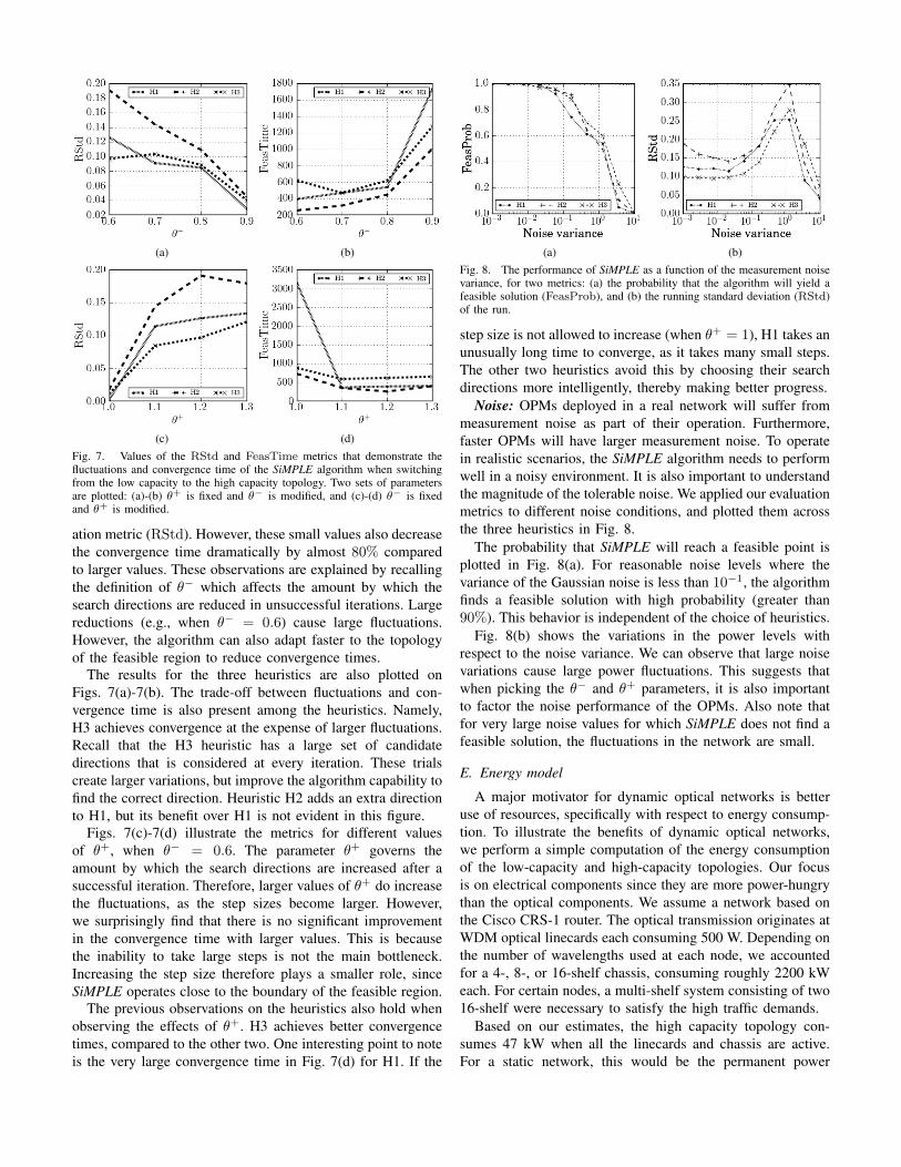
Figs. 7(a)-7(b) show the effect of the θ− parameter whenθ+ = 1.2. One can notice that smaller values of θ− causelarger fluctuations, as measured by the running standard devi-

(a) (b)

(c) (d)Fig. 7. Values of the RStd and FeasTime metrics that demonstrate thefluctuations and convergence time of the SiMPLE algorithm when switchingfrom the low capacity to the high capacity topology. Two sets of parametersare plotted: (a)-(b) θ+ is fixed and θ− is modified, and (c)-(d) θ− is fixedand θ+ is modified.

ation metric (RStd). However, these small values also decreasethe convergence time dramatically by almost 80% comparedto larger values. These observations are explained by recallingthe definition of θ− which affects the amount by which thesearch directions are reduced in unsuccessful iterations. Largereductions (e.g., when θ− = 0.6) cause large fluctuations.However, the algorithm can also adapt faster to the topologyof the feasible region to reduce convergence times.

The results for the three heuristics are also plotted onFigs. 7(a)-7(b). The trade-off between fluctuations and con-vergence time is also present among the heuristics. Namely,H3 achieves convergence at the expense of larger fluctuations.Recall that the H3 heuristic has a large set of candidatedirections that is considered at every iteration. These trialscreate larger variations, but improve the algorithm capability tofind the correct direction. Heuristic H2 adds an extra directionto H1, but its benefit over H1 is not evident in this figure.

Figs. 7(c)-7(d) illustrate the metrics for different valuesof θ+, when θ− = 0.6. The parameter θ+ governs theamount by which the search directions are increased after asuccessful iteration. Therefore, larger values of θ+ do increasethe fluctuations, as the step sizes become larger. However,we surprisingly find that there is no significant improvementin the convergence time with larger values. This is becausethe inability to take large steps is not the main bottleneck.Increasing the step size therefore plays a smaller role, sinceSiMPLE operates close to the boundary of the feasible region.

The previous observations on the heuristics also hold whenobserving the effects of θ+. H3 achieves better convergencetimes, compared to the other two. One interesting point to noteis the very large convergence time in Fig. 7(d) for H1. If the

(a) (b)Fig. 8. The performance of SiMPLE as a function of the measurement noisevariance, for two metrics: (a) the probability that the algorithm will yield afeasible solution (FeasProb), and (b) the running standard deviation (RStd)of the run.

step size is not allowed to increase (when θ+ = 1), H1 takes anunusually long time to converge, as it takes many small steps.The other two heuristics avoid this by choosing their searchdirections more intelligently, thereby making better progress.

Noise: OPMs deployed in a real network will suffer frommeasurement noise as part of their operation. Furthermore,faster OPMs will have larger measurement noise. To operatein realistic scenarios, the SiMPLE algorithm needs to performwell in a noisy environment. It is also important to understandthe magnitude of the tolerable noise. We applied our evaluationmetrics to different noise conditions, and plotted them acrossthe three heuristics in Fig. 8.

The probability that SiMPLE will reach a feasible point isplotted in Fig. 8(a). For reasonable noise levels where thevariance of the Gaussian noise is less than 10−1, the algorithmfinds a feasible solution with high probability (greater than90%). This behavior is independent of the choice of heuristics.

Fig. 8(b) shows the variations in the power levels withrespect to the noise variance. We can observe that large noisevariations cause large power fluctuations. This suggests thatwhen picking the θ− and θ+ parameters, it is also importantto factor the noise performance of the OPMs. Also note thatfor very large noise values for which SiMPLE does not find afeasible solution, the fluctuations in the network are small.

E. Energy model

A major motivator for dynamic optical networks is betteruse of resources, specifically with respect to energy consump-tion. To illustrate the benefits of dynamic optical networks,we perform a simple computation of the energy consumptionof the low-capacity and high-capacity topologies. Our focusis on electrical components since they are more power-hungrythan the optical components. We assume a network based onthe Cisco CRS-1 router. The optical transmission originates atWDM optical linecards each consuming 500 W. Depending onthe number of wavelengths used at each node, we accountedfor a 4-, 8-, or 16-shelf chassis, consuming roughly 2200 kWeach. For certain nodes, a multi-shelf system consisting of two16-shelf were necessary to satisfy the high traffic demands.

Based on our estimates, the high capacity topology con-sumes 47 kW when all the linecards and chassis are active.For a static network, this would be the permanent power

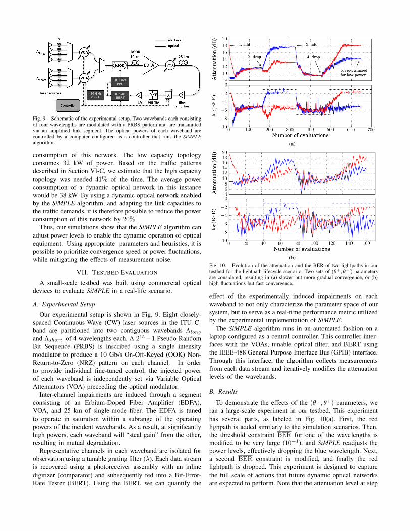
Fig. 9. Schematic of the experimental setup. Two wavebands each consistingof four wavelengths are modulated with a PRBS pattern and are transmittedvia an amplified link segment. The optical powers of each waveband arecontrolled by a computer configured as a controller that runs the SiMPLEalgorithm.

consumption of this network. The low capacity topologyconsumes 32 kW of power. Based on the traffic patternsdescribed in Section VI-C, we estimate that the high capacitytopology was needed 41% of the time. The average powerconsumption of a dynamic optical network in this instancewould be 38 kW. By using a dynamic optical network enabledby the SiMPLE algorithm, and adapting the link capacities tothe traffic demands, it is therefore possible to reduce the powerconsumption of this network by 20%.

Thus, our simulations show that the SiMPLE algorithm canadjust power levels to enable the dynamic operation of opticalequipment. Using appropriate parameters and heuristics, it ispossible to prioritize convergence speed or power fluctuations,while mitigating the effects of measurement noise.

VII. TESTBED EVALUATION

A small-scale testbed was built using commercial opticaldevices to evaluate SiMPLE in a real-life scenario.

A. Experimental Setup

Our experimental setup is shown in Fig. 9. Eight closely-spaced Continuous-Wave (CW) laser sources in the ITU C-band are partitioned into two contiguous wavebands–Λlongand Λshort–of 4 wavelengths each. A 215−1 Pseudo-RandomBit Sequence (PRBS) is inscribed using a single intensitymodulator to produce a 10 Gb/s On-Off-Keyed (OOK) Non-Return-to-Zero (NRZ) pattern on each channel. In orderto provide individual fine-tuned control, the injected powerof each waveband is independently set via Variable OpticalAttenuators (VOA) preceeding the optical modulator.

Inter-channel impairments are induced through a segmentconsisting of an Erbium-Doped Fiber Amplifier (EDFA),VOA, and 25 km of single-mode fiber. The EDFA is tunedto operate in saturation within a subrange of the operatingpowers of the incident wavebands. As a result, at significantlyhigh powers, each waveband will “steal gain” from the other,resulting in mutual degradation.

Representative channels in each waveband are isolated forobservation using a tunable grating filter (λ). Each data streamis recovered using a photoreceiver assembly with an inlinedigitizer (comparator) and subsequently fed into a Bit-Error-Rate Tester (BERT). Using the BERT, we can quantify the

(a)

(b)Fig. 10. Evolution of the attenuation and the BER of two lightpaths in ourtestbed for the lightpath lifecycle scenario. Two sets of (θ+, θ−) parametersare considered, resulting in (a) slower but more gradual convergence, or (b)high fluctuations but fast convergence.

effect of the experimentally induced impairments on eachwaveband to not only characterize the parameter space of oursystem, but to serve as a real-time performance metric utilizedby the experimental implementation of SiMPLE.

The SiMPLE algorithm runs in an automated fashion on alaptop configured as a central controller. This controller inter-faces with the VOAs, tunable optical filter, and BERT usingthe IEEE-488 General Purpose Interface Bus (GPIB) interface.Through this interface, the algorithm collects measurementsfrom each data stream and iteratively modifies the attenuationlevels of the wavebands.

B. Results

To demonstrate the effects of the (θ−, θ+) parameters, weran a large-scale experiment in our testbed. This experimenthas several parts, as labeled in Fig. 10(a). First, the redlighpath is added similarly to the simulation scenarios. Then,the threshold constraint BER for one of the wavelengths ismodified to be very large (10−1), and SiMPLE readjusts thepower levels, effectively dropping the blue wavelength. Next,a second BER constraint is modified, and finally the redlightpath is dropped. This experiment is designed to capturethe full scale of actions that future dynamic optical networksare expected to perform. Note that the attenuation level at step

5 on Fig.10(a) is larger compared to that just before step 2,even though their BER levels are the same. This shows thatthe same QoT constraint can be met using less optical power.

We ran this experiment over different values of θ− and θ+.We show two sample outcomes in Fig. 10. Fig 10(b) showsthe variations of the power level and the corresponding BERwhen θ− = 0.6 and θ+ = 1.2. Similar to the insight obtainedfrom simulations, these parameters cause large variations inthe step size, leading to large fluctuations in the power levelsand the BER. However, these parameters also allow the entiretest sequence to complete in about 170 OPM evaluations.

Fig 10(a) corresponds to the same scenario with θ− = 0.9and θ+ = 1. It can be seen that the variations in power andBER are much lower, and the convergence is smoother. Thissmoothness comes at a penalty in time since the entire sce-nario takes about 650 OPM evaluations. As future OPMs areexpected to perform evaluations in the order of milliseconds,the SiMPLE algorithm can complete this scenario in under asecond, with reasonable convergence behavior.

To conclude, we tested our algorithm running on a computerthat controlled on optical devices. We showed that the insightsfrom simulations also hold with real equipment, and thatproper selection of parameters for the SiMPLE Algorithm canenable complex operations in future dynamic optical networks.

VIII. CONCLUSION

In this paper, we formulated a global optimization problem,MLO, that captures the QoS guarantees of optical networks.This problem is unique since there do not exist analyticalmodels that capture impairments in optical fibers, and mea-surements are the only practical way to characterize perfor-mance. We designed a global network management algorithm,SiMPLE, for solving this problem by using feedback from real-life OPMs. The convergence of SiMPLE to the optimal solu-tion is demonstrated using extensive simulations on a network-wide optical network simulator, as well as measurements withcommercial optical network equipment. We showed that evensimple dynamic policies in optical networks can result insubstantial power savings through a better use of resources.

The SiMPLE algorithm enables dynamic control of opticalnetworks in near real-time. Compared to the days-long setuptimes for lightpaths in current optical networks, using SiMPLEis the first step in allowing optical networks to react rapidly touser demands and traffic variations, and can lead to a software-defined optical network. In future work, we will investigatecontrolling modulation schemes and the optical bandwidth aspart of this dynamic network control plane.

ACKNOWLEDGEMENTS

This work was supported in part by CIAN NSF ERC under grantEEC-0812072, NSF grant CNS-1018379, and DTRA grant HDTRA1-13-1-0021. This material is based upon work supported by (whileone of the authors was serving at) the National Science Foundation.Any opinion, findings and conclusions or recommendations expressedhere do not necessarily reflect the views of the National ScienceFoundation.

REFERENCES

[1] “Cisco impairment-aware WSON control plane,” http://www.cisco.com/en/US/prod/collateral/optical/ps5724/ps2006/data sheet c78-689160.html.

[2] “Geant project,” http://www.geant.net.[3] “Cisco visual networking index: Forecast and methodology, 2011-2016,”

White Paper, 2012.[4] Proc. IEEE, Special Issue on The Evolution of Optical Networking, vol.

100, no. 5, May 2012.[5] S. Azodolmolky, M. Klinkowski, E. Marin, D. Careglio, J. S. Pareta, and

I. Tomkos, “A survey on physical layer impairments aware routing andwavelength assignment algorithms in optical networks,” Comput. Netw.,vol. 53, no. 7, pp. 926–944, 2009.

[6] B. Birand, H. Wang, K. Bergman, and G. Zussman, “Measurements-based power control – a cross-layered framework,” in Proc. OFC’13,Mar. 2013.

[7] C. Chekuri, P. Claisse, R.-J. Essiambre, S. Fortune, D. C. Kilper, W. Lee,N. K. Nithi, I. Saniee, B. Shepherd, C. A. White, G. Wilfong, andL. Zhang, “Design tools for transparent optical networks,” Bell LabsTech. J., vol. 11, no. 2, pp. 129–243, 2006.

[8] A. Conn, K. Scheinberg, and L. Vicente, Introduction to derivative-freeoptimization. Society for Industrial Mathematics, 2009, vol. 8.

[9] R. Doverspike and J. Yates, “Optical network management and control,”Proc. IEEE, vol. 100, no. 5, pp. 1092–1104, May 2012.

[10] D. J. Geisler, R. Proietti, Y. Yin, R. P. Scott, X. Cai, N. K. Fontaine,L. Paraschis, O. Gerstel, and S. J. B. Yoo, “Experimental demonstrationof flexible bandwidth networking with real-time impairment awareness,”Opt. Express, no. 26, pp. B736–B745, Dec. 2011.

[11] O. Gerstel, M. Jinno, A. Lord, and S. Yoo, “Elastic optical networking:a new dawn for the optical layer?” IEEE Commun. Mag., vol. 50, no. 2,pp. s12–s20, Feb. 2012.

[12] M. S. Islam and S. P. Majumder, “Bit error rate and cross talkperformance in optical cross connect with wavelength converter,” J. Opt.Netw., vol. 6, no. 3, pp. 295–303, Mar. 2007.

[13] D. Kilper, K. Guan, K. Hinton, and R. Ayre, “Energy challenges incurrent and future optical transmission networks,” Proc. IEEE, vol. 100,no. 5, pp. 1168–1187, May 2012.

[14] C. Lai, A. Fard, B. Buckley, B. Jalali, and K. Bergman, “Cross-layersignal monitoring in an optical packet-switching test-bed via real-timeburst sampling,” in Proc. IPC’10, Nov. 2010.

[15] Y. Lee, G. Bernstein, D. Li, and G. Martinelli, “A framework forthe control of wavelength switched optical networks (WSONs) withimpairments,” Internet Engineering Task Force, RFC 6566, Mar. 2012.

[16] E. Mannie, “Generalized Multi-Protocol label switching (GMPLS) ar-chitecture,” Internet Engineering Task Force, RFC 3945, Oct. 2004.

[17] G. Martinelli, “GMPLS Signaling Extensions for Optical ImpairmentAware Lightpath Setup,” Internet Engineering Task Force,Internet-Draft, 2010. [Online]. Available: http://tools.ietf.org/html/draft-martinelli-ccamp-optical-imp-signaling-03.txt

[18] B. Mukherjee, Optical WDM networks. Springer-Verlag New York Inc,2006.

[19] J. Nocedal and S. Wright, Numerical optimization. Springer-Verlag,1999.

[20] Y. Pan, T. Alpcan, and L. Pavel, “A system performance approach toOSNR optimization in optical networks,” IEEE Trans. Commun., vol. 58,no. 4, pp. 1193–1200, Apr. 2010.

[21] Z. Pan, C. Yu, and A. Willner, “Optical performance monitoring forthe next generation optical communication networks,” Optical FiberTechnology, vol. 16, no. 1, pp. 20–45, 2010.

[22] R. Ramaswami, K. Sivarajan, and G. Sasaki, Optical networks: apractical perspective. Morgan Kaufmann, 2009.

[23] J. Sole-Pareta, S. Subramaniam, D. Careglio, and S. Spadaro, “Cross-layer approaches for planning and operating impairment-aware opticalnetworks,” Proc. IEEE, vol. 100, no. 5, pp. 1118–1129, May 2012.

[24] S. Uhlig, B. Quoitin, J. Lepropre, and S. Balon, “Providing public in-tradomain traffic matrices to the research community,” ACM SIGCOMMComput. Commun. Rev., vol. 36, no. 1, pp. 83–86, 2006.

[25] S. Woodward and M. Feuer, “Toward more dynamic optical networking,”in Proc. OECC’10, July 2010.

[26] Y. Wu, L. Chiaraviglio, M. Mellia, and F. Neri, “Power-aware routingand wavelength assignment in optical networks,” in Proc. ECOC’09,Sept. 2009.