Real-time Tactical and Strategic Sales Management for Intelligent

Agents Guided By Economic Regimes

Wolfgang Ketter†, John Collins, Maria Gini, Alok Gupta⋆, and Paul Schrater

Computer Science and Engineering, University of Minnesota†Rotterdam Sch. of Mgmt., Erasmus University⋆Carlson Sch. of Mgmt., University of Minnesota

wketter@rsm.nl, [jcollins, gini, schrater]@cs.umn.edu, alok@umn.edu

Abstract

Many enterprises that participate in dynamic markets need to make product pricing and inven-

tory resource utilization decisions in real-time. We describe a family of statistical models that address

these needs by combining characterization of the economic environment with the ability to predict fu-

ture economic conditions to make tactical (short-term) decisions, such as product pricing, and strategic

(long-term) decisions, such as level of finished goods inventories. Our models characterize economic

conditions, called economic regimes, in the form of recurrent statistical patterns that have clear quali-

tative interpretations. We show how these models can be used to predict prices, price trends, and the

probability of receiving a customer order at a given price. These “regime” models are developed using

statistical analysis of historical data, and are used in real-time to characterize observed market conditions

and predict the evolution of market conditions over multiple time scales. We evaluate our models using

a testbed derived from the Trading Agent Competition for Supply Chain Management (TAC SCM), a

supply chain environment characterized by competitive procurement and sales markets, and dynamic

pricing. We show how regime models can be used to inform both short-term pricing decisions and long-

term resource allocation decisions. Results show that our method outperforms more traditional short-

and long-term predictive modeling approaches.

Keywords: Agent-mediated electronic commerce, dynamic pricing, enabling technologies, price forecasting,

economic regimes, supply-chain, dynamic markets, Trading Agent Competition

1 Introduction

To seek competitive advantage, firms are employing increasingly sophisticated automated decision support

systems. These advanced decision support systems often involve designing software agents that can act

rationally on behalf of their users or assist the users in a variety of application areas. Examples include

procurement (Sandholm, 2007), scheduling and resource management (Collins et al., 2002), and personal

information management (Berry et al., 2006; Mark and Perrault, 2006). Software agents have the advantage

of being able to analyze many more possibilities in shorter time frames than their human counterparts, but

are often limited in their ability to make strategic decisions. In this paper we present computational methods

1

for a software agent that considers long-term expected profit implications when making short-term tactical

decisions, such as setting current prices and quantities of products to sell in a given time-frame.

We look at a complex and critical part of the supply chain relating to product pricing decisions in an auction

based dynamic pricing environment where customer demand is stochastic. We are particularly interested in

multi-commodity supply-chain environments that are constrained by capacity and materials availability and

where market conditions may be characterized qualitatively, for example, by over-supply or scarcity. Such

environments exist in business-to-business (B2B) exchanges where several suppliers compete for business from

customers for commoditized manufactured parts (Kaplan and Sawhney, 2000). Given the rapid increase in

implementations of technology assisted market based mechanisms, in the near future such environments are

likely to develop for more complex products.

One of the innovative and unique characteristics of our approach is to make pricing decisions not just based

on current demand but on anticipated future demand and other hidden factors, which are aggregated by

assessing the “economic regimes” and their expected future transitions. Economic regimes characterize

market conditions by detecting distinguishable statistical patterns in historical market data. They capture

overall market conditions, such as scarcity or oversupply, and provide valuable indications such as price trend

and price distribution predictions over a planning horizon. In this work, we focus on observable pricing data

as a surrogate for a range of typically hidden variables that affect pricing decisions of buyers and sellers in

a market.

In previous research (Ketter et al., 2009) we proposed the use of economic regimes and shown how to identify

them from historical data. However, we did not address whether regime predictions can be made for new

unseen environments. Further it was not clear how managerial decisions such as pricing, sales quota, and

profits could benefit from the knowledge of economic regime forecasts. These issues are addressed in this

paper, where we present new methods to identify in real-time economic regimes and to predict future regime

transitions and related future price distributions and price trends. Our computational approaches are light-

weight, i.e., designed to operate with minimal computational burden so that they can respond to requests

in real-time.

Further, we develop a model that uses regime predictions to set sales quotas for current and future sales

with the objective of maximizing profit over time. Our approach is tested by embedding our computational

methods in a software agent that operates in the Trading Agent Competition for Supply Chain Management

(TAC SCM) (Collins et al., 2010b). Experimental results show that our approach performs better than

traditional predictive modeling methods.

While predictions about the economic environment are commonly made at the macroeconomic level (Osborn

and Sensier, 2002), to our knowledge, such predictions are rarely done for microeconomic environments and

represent a novel contribution of this research. In addition, systemic use of these forecasts for decision

making is also a unique contribution of this research. Our previous work (Ketter et al., 2009) focused on

using economic regimes for their explanatory power, whereas this paper focuses on their predictive power.

This distinction is central to the current debate on explanatory vs. predictive modeling (Shmueli, 2010).

Economic regimes can be used to support decisions in both procurement and sales markets. In the procure-

ment market, we may have little or no control over the availability of parts, but we can control the usable

supply to a certain degree. Prices increase when there is scarcity. Scarcity of parts commonly results from

excess demand, which tends to occur when demand for associated products is high. This is precisely why

prediction of regimes is important. If we can predict an increase in prices of finished products, then we may

2

decide to acquire parts early, thereby reducing cost of material and increasing our profit margin.

The approach we present is applicable also to commodity markets for items such as cotton, oil, or semicon-

ductor chips, where fast changing market conditions and high price volatility are common. For example, the

procurement risk management process at Hewlett-Packard (Nagali et al., 2008) uses probabilistic estimates

of future price, demand, and supply to forecast a range of future market scenarios, which are in turn used to

evaluate potential procurement contracts. This process has saved Hewlett-Packard hundreds of millions of

dollars in the procurement of flash memory alone. Although Nagali et al. (2008) do not describe their price

prediction model in detail, the regime-based model we describe in this paper produces a probabilistic esti-

mate of future prices that could be used in such a system. Our results show that even though a market may

be constantly changing, there are some underlying dominant patterns or economic regimes that characterize

market conditions.

The paper is organized as follows. In Section 2 we review relevant literature. Section 3 describes the

foundations of our economic regime approach. It shows how to make real-time predictions about future

economic regimes and price distributions, and how economic regimes can support strategic and tactical sales

decisions. Section 4 describes our testbed, the Trading Agent Competition for Supply-Chain Management

(TAC SCM). In Section 5 we present experimental results using the TAC SCM testbed. Finally, we conclude

with directions for future research.

2 Background and Literature Review

Pricing of products to retailers or distributors is a key aspect of supply chain management for any profit

maximizing firm. Most studies (e.g., (Cachon and Netessine, 2004; Kleindorfer and Wu, 2003)) look at this

issue in a single supplier and single buyer setting, due to analytical complexity and tractability issues. While

dynamic pricing is seen as a potentially superior approach (Elmaghraby and Keskinocak, 2003; Swaminathan

and Tayur, 2003), the market power, and thus the power to set prices, is still assumed to be with the supplier

or manufacturer. However, information systems researchers have started looking at the potential of dynamic

pricing through auction based approaches to provide incentives for supply chain coordination (e.g., (Fan

et al., 2003)). Our approach is based on the assumption that competitive markets where manufacturers

compete for customers’ business will eventually lead to dynamic pricing, in which prices will emerge from

interactions between manufacturers and their customers.

Various methods to predict prices have been used, such as in first price sealed bid reverse auctions for

IBM PCs (Lawrence, 2003), PDAs on eBay (Ghani, 2005), or in predicting ending prices for a multi-unit

online ascending auction (Bapna et al., 2008). Dynamic forecasting of auction bidding prices is becoming

increasingly popular because of the massive use of online auctions (Wang et al., 2008). Short-term price

prediction has been the focus of several studies where prices move primarily due to demand-side constraints,

such as in the electricity market (Nogales et al., 2002). Specific methods for price prediction in TAC SCM

are covered later in Section 4.1.

While approaches to price prediction vary considerably, it is widely recognized that predictions need to exploit

the information available in the market and to take its structure into account (Muth, 1961). However, as Gray

and Spencer (1990) note, demand-side price movements are intrinsically linked with supply side movements.

Massey and Wu (2005) show that the ability of decision makers to correctly identify the onset of a new

regime can mean the difference between success and failure. Furthermore, they found strong evidence that

3

individuals pay inordinate attention to the signal (price in our case), and neglect the aspects of the system

that generate the signal (regime dynamics). This results in a tendency to over- or under-react to market

conditions.

Several researchers have identified the existence and cyclic nature of economic regimes in consumer markets.

For example, Ghose et al. (2006) empirically analyze the degree to which used products cannibalize new

product sales for books on Amazon.com and show that product prices go through different regimes over

time. Similarly, Pauwels and Hanssens (2002) analyze how strategic windows of change alternate with long

periods of stability in mature economic markets.

In this paper we develop computationally efficient methods to identify and predict economic regimes that can

be used by decision makers or by autonomous computational agents to make pricing decisions in a complex

supply-chain environment. Our method is able to detect and forecast a broad range of market conditions.

Regression based approaches (including non-parametric variations) assume that the functional form of the

relationship between dependent and independent variables has a consistent structure across the range of

market conditions. In contrast, our approach models variability in market conditions and does not assume

a functional relationship; this allows detection of changes in relationship between prices and sales over time.

3 Economic regimes for real-time prediction of price distributions

We now describe the details of our approach. Any economic decision process should account for prevailing and

future market conditions since these changing conditions affect an organization’s strategies for procurement,

production planning, and pricing. These market conditions can be broadly defined as scarcity, balanced,

and oversupply. A scarcity condition exists when demand exceeds product supply in the market, a balanced

condition when demand is approximately equal to supply, and an oversupply condition when supply exceeds

demand. When there is scarcity, firms have pricing power and may price more aggressively. In balanced

situations, prices have some spread, so firms have a range of options for maximizing expected profit. In

oversupply situations, prices are lower and firms should primarily control costs, and therefore either price

based on costs, or conserve resources for better market conditions.

As indicated earlier, we assume that observable prices act as signals of the underlying true state of the

economy, and we use them to estimate future regimes, from which we can then estimate price trends and

price distributions. Our regime model is a Hierarchical Hidden Markov Model (HHMM) (Fine et al., 1998).

A HHMM allows for the existence of hidden, as well as observable, parameters. Price is an observable

parameter whose changes drive a hidden “state” (economic regime) of the economy.

Overall, the computational approaches we present are able to:

1. identify the current economic regime using price history and real-time data;

2. estimate future regimes of the market, specifically regime distributions, price density, price trends, and

probability of receiving orders at a given price;

3. make dynamic decisions on what products to sell and at what price using the predictions.

4

3.1 Background

We focus our work on an exchange marketplace that is characterized by several competing firms offering

several identical products; since the products are identical, customers buying decisions are only based on

price. We assume that during each discrete planning period (which we call “day”) each firm decides whether

or not to offer a product and set an appropriate price for each product that is offered. Such decisions require

projecting future customer demand along with a given firm’s inventory levels, production capacity, and other

necessary resources.

For simplicity, we aggregate price data for different goods. Since prices may have different ranges for different

products, we normalize them by dividing the price of a good by the nominal cost of its components and the

variable assembly cost. We assume prices are dynamic and change every day according to market conditions.

We define the normalized price for good g on day d as npd,g = priced,g/(nominal cost(Cg) + assembly costg).

where Cg is the set of components in product g. In the following, for simplicity of notation, we use np instead

of npd,g, unless there is ambiguity.

We briefly summarize the theory of economic regimes (Ketter et al., 2009) as a foundation for the rest of this

paper. Instead of assuming a given distribution for prices, we approximate an arbitrary price distribution

by fitting a Gaussian mixture model (GMM) (Titterington et al., 1985) to historical normalized price data.

The demand characteristics in electronic marketplaces have been found to be fractal, that is the short-term

demand pattern has much larger variation than the long-term time-averaged demand pattern (Gupta et al.,

1997). This means that while there are periods of no or little demand there will be periods when demand

will be extremely high. The pricing strategy needs to take this into account. Typically, parameterized econo-

metric models perform poorly in these situations. In contrast, non-parametric approaches do an excellent

job in estimation, but usually are computationally too expensive. In our testbed and in many real-world

trading scenarios, decisions have to be made quickly and there is no time for time consuming calculations.

Therefore, we decided to adopt a semi-parametric approach, and in particular the GMM, which can be

computed efficiently and uses less memory than other approaches1.

We use the Expectation-Maximization (EM) algorithm (Dempster et al., 1977) to determine the prior prob-

ability, P (ζi), of each Gaussian component ζi of the GMM. The prior probabilities of these Gaussian compo-

nents determine the amplitude of a particular Gaussian, and the sum over all Gaussians results in a GMM

which fits the underlying data. The density of the normalized price can be written as:

p(np) =N∑i=1

p(np|ζi)P (ζi) (1)

where N is the number of Gaussians in the mixture model and p(np|ζi) is the contribution of the i-th

Gaussian to the normalized price density. The number of Gaussians has to be chosen to balance two

conflicting requirements: too many Gaussians will overfit the data and result in a model that does not

generalize, while too few will provide a crude and inaccurate estimate.

Using Bayes’ rule we determine the posterior probabilities for each Gaussian ζi. We then define the pos-

terior probabilities of all Gaussians given the normalized price np as the N -dimensional vector η(np) =

[P (ζ1|np), P (ζ2|np), . . . , P (ζN |np)]. For each observed normalized price npj we compute the vector of the

posterior probabilities, η(npj), which is η evaluated at each observed normalized price npj . Intuitively, the

1For a more detailed discussion of the choice and advantages of the chosen modeling approach related to real-time adaptation

and decision-making please see the online appendix.

5

idea of a regime as a recurrent economic condition is captured by discovering price distributions that recur

across time periods in the market. We define regimes by clustering price distributions over time periods

using the k-means algorithm. The clusters found correspond to frequently occurring price distributions with

support on contiguous ranges of np. The center of each cluster is a probability vector that corresponds to

a regime Rk, for k = 1, · · · ,M , where M is the number of regimes. Collecting these vectors into a matrix

yields the conditional probability matrix P(ζ|R). After we marginalize over all Gaussians ζi we obtain the

density of the normalized price np dependent on regime Rk as:

p(np|Rk) =

N∑i=1

p(np|ζi)P (ζi|Rk). (2)

The probability of regime Rk dependent on the normalized price np can then be computed using Bayes’ rule

as:

P (Rk|np) =p(np|Rk)P (Rk)∑Mi=1 p(np|Ri)P (Ri)

for k = 1, · · · ,M (3)

where M is the number of regimes. The prior probabilities, P (Rk), of the regimes are determined by a

counting process over historical data.

At any given time, one of the regimes Rk will typically have a higher probability than the others. Eco-

nomically, it is common to think in terms of three dominant regimes (scarcity, balanced, and oversupply);

however, estimating a larger number of regimes can generate additional insights into market conditions,

such as extreme oversupply and extreme scarcity. We conducted several experiments varying the number

of regimes between three and 10, and discovered that three and five regimes provide the best tradeoff in

terms of predictive and explanatory power (Shmueli, 2010), and computational load. We use a five regime

model because the extreme cases (extreme oversupply and extreme scarcity) represent qualitatively distinct

market conditions, and are therefore important distinctions for decision making. Mathematical details for

computing both the optimal number of Gaussians and of regimes are presented in Ketter (2007); Ketter

et al. (2009). and in the online appendix.

Next we present the computational machinery for real-time predictions, before demonstrating its effectiveness

in the TAC SCM environment in Section 5.

3.2 Real-time prediction methods

In this section, we describe three different regime prediction methods. The first is based on exponential

smoothing, the second is a Markov prediction process, and the last is a Markov correction-prediction process.

Each of these methods has different strengths and should be used in different circumstances. The exponential

smoother is ideal to estimate the current regime distribution, since it makes predictions using only information

about the recent past, making it more reactive to the current market condition. The Markov prediction

process is appropriate for short- and mid-term predictions, while the Markov correction-prediction process

is suited for long-term predictions.

3.2.1 Exponential smoother price prediction

Using an estimate of the mean normalized price npd,g (or the actual mean of the normalized price npd,g if

available) for each good g on day d we can compute the price trend and use it to predict future prices. For

6

consistency with the TAC SCM case study we present later, we use the term “day” to refer to a discrete

planning period of arbitrary size and we use an estimate of the mean price because the actual mean price is

not observable in many markets, including TAC SCM.

Since prices tend to be noisy and both mean and trend vary over time, an exponential smoother can be used

to generate short-term predictions from recent observations. Specifically, we use a Brown linear exponential

smoothing (Brown et al., 1961), which uses two different smoothed series centered at different points in

time and a forecasting formula based on an extrapolation of a line through the two centers. The smoothed

normalized mean price is computed using np′and np

′′, respectively the singly-smoothed and doubly-smoothed

normalized mean price estimates, as follows:

npd−1 = 2np′d−1 − np

′′d−1 (4)

where

np′d−1 = β · npd−1 + (1− β) · np′d−2 (5)

np′′d−1 = β · np′d−1 + (1− β) · np′′d−2 (6)

The model can be initialized simply by setting both smoothed series equal to the observed value at d = 1. The

parameter β ∈ (0, 1) provides computational stability in prediction between the two exponentially smoothed

time series. We determined the value of β using a hill-climbing process to minimize prediction error over a

set of historical data, and selected β = 0.5. We will show later in Section 5.1 how we compute a smoothed

mean price estimate in TAC SCM where the only information available are the minimum and maximum

price for the previous day.

We then compute the smoothed price trend as:

trd−1 =β

1− β· (np′d−1 − np

′′d−1) (7)

Using the trend and the previous day’s smoothed mean price npd−1 we predict the daily smoothed prices

from the current day d for each day n over the horizon h as:

npd+n = npd−1 + (1 + n) · trd−1, for n = 1, · · · , h (8)

The predicted prices, npd+n, over the planning horizon h are used as input for the exponential smoother

regime prediction, which is described next. In contrast, both Markov regime prediction methods (described

later) use only use previous day’s estimated price, npd−1, as input and make predictions using Markov

transition matrices that are computed from historical data.

3.2.2 Exponential smoother regime prediction

The exponential smoother prediction process we described yields estimates of future mean prices, but no

information on price distributions. To obtain price distributions we translate the estimates of future prices

to regime predictions and then we predict price distributions from regimes (see Section 3.3). As we shall see

later in Section 5.3.2, doing so actually improves price predictions as well.

Using the predicted mean price npd+n computed with (8), we obtain the density of npd+n dependent on

regime Rk using (2), and the predicted probability of regime Rk dependent on the predicted normalized

7

price n days into the future, npd+n, using (3). Note that we use Rk to denote a particular predicted regime

Rk.

Since the regime information is obtained from historical data, prices and corresponding regime probabilities

can be computed in advance and stored in a table, reducing the subsequent real-time computations to a

table lookup. This predictor is not as flexible as the others we will describe next, since it does not learn

patterns in the data, but it is easy to compute. We use the term “exponential smoother with regimes” to

describe this combination of using the exponential smoother to predict prices and then a table lookup to

find the corresponding regime probabilities.

3.2.3 Markov regime prediction

We model the short-term prediction of future regimes as a Markov prediction (Markov P) process. The

prediction is based only on the most recent price npd−1 and on historical data. We first compute a Markov

transition matrix for regime transitions, T(rd+n|rd−1), by a counting process using historical data. This

matrix represents the posterior probability of transitioning from regime rd−1 on day d − 1 to regime rd+n

on day d + n, where r = Rk for k = 1, · · · ,M , and M is the number of regimes. We use P (rd−1|npd−1) to

indicate a M-dimensional vector of the posterior probabilities of the predicted regimes r on day d− 1.

We further distinguish between two types of Markov predictions: (1) n-day, and (2) repeated 1-day prediction.

An n-day prediction computes a transition matrix for each of the n days in the future and multiplies these

matrices by the current day regime estimates to predict regimes n-days in the future. The repeated 1-day

matrix instead assumes a stable transition matrix and multiplies itself n times to produce the transition

probabilities for n-days in the future.

The prediction of the posterior distribution of regimes n days into the future, P (rd+n|npd−1), is done recur-

sively as follows:

1. n-day prediction. The n-day prediction is based on training a separate Markov transition matrix for

each day in the planning horizon h, i.e. Tn(rd+n|rd−1), for n = 1, · · · , h.

P (rd+n|npd−1) = Tn(rd+n|rd−1) P (rd−1|npd−1) forn = 1, . . . , h (9)

2. Repeated 1-day prediction. The repeated 1-day prediction is done by using the 1-day prediction matrix

T1(rd|rd−1) multiple times.

P (rd+n|npd−1) =n∏

T1(rd|rd−1) P (rd−1|npd−1) forn = 1, . . . , h (10)

In a completely stable environment, n repeated 1-day Markov predictions would lead to the same results

as a single application of the appropriate n-day prediction. In real environments, however, this assumption

is often violated, since the environment changes dynamically over time. When making predictions far in

the future, the repeated 1-day method reaches a stationary distribution where all transition probabilities

converge to the same values. This drawback can be avoided by using a n-day Markov prediction matrix.

Details can be found in the online appendix.

The prior regime probability for the first day needs to be assigned according to the market situation. For

instance, in TAC SCM we set the prior regime probability for the first day to 100% extreme scarcity, to

represent the condition when the initial finished product inventories are zero.

8

3.2.4 Markov regime correction-prediction

For long-term prediction of future regimes we use a Markov correction-prediction (Markov C-P) process,

where the prediction part is similar to the Markov prediction described above but taking into account the

entire real-time price history, np1, . . . , npd−1, instead of a single day npd−1. A Markov correction-prediction

process is better when the process depends on real-time transitions in the immediate past beyond a single

day. Both Markov P and Markov C-P processes depend on either 1-day or n-day transition matrices which

are learned offline from historical data. The Markov C-P method is based on two distinct operations done

in sequence:

1. a correction (recursive Bayesian update) of the posterior probabilities of the regimes based on the

history of prices starting from the first, np1, until the most recent on day d− 1 is given by:

P (rd−1|{np1, . . . , npd−1}) =P (npd−1|rd−1) P (rd−1|{np1, . . . , npd−2})∑M

rd−1=1 P (npd−1|rd−1) P (rd−1|{np1, . . . , npd−2})(11)

2. a prediction of the posterior probabilities of regimes n days into the future, P (rd+n|{np1, . . . , npd−1}),is done recursively as in the Markov prediction case. The n-day prediction is given by

P (rd+n|{np1, . . . , npd−1}) = Tn(rd+n|rd−1) P (rd−1|{np1, . . . , npd−1}) forn = 1, . . . , h (12)

The repeated one-day prediction is given by

P (rd+n|{np1, . . . , npd−1}) =n∏

T1(rd|rd−1) P (rd−1|{np1, . . . , npd−1}) forn = 1, . . . , h (13)

Note that Eq. 12 and Eq. 13 use a matrix multiplication, whereas Eq. 11 uses an element wise multiplication.

3.2.5 Computational complexity of economic regimes

The key computational requirements of the regime model’s price predictions involve propagating the hidden

state density forward, called forward filtering. Forward filtering has well-known computational complexity

results, with time complexity of O(M2T ) and memory complexity of O(MT ) (Khreich et al., 2010), where

M is the number of regimes, and T is the number of time steps used for making a prediction. For our Markov

P process T is the number of forecast steps, and for the Markov C-P process it is the entire history plus

the number of extrapolated steps. The dependence on time reflects the fact that the algorithm takes the

entire history of the sequence into account when making predictions, while the quadratic dependence on the

regime state size is due to the matrix multiplication used to propagate regime state probabilities. These worst

case results can potentially be improved by limiting the data history the algorithm processes before making

predictions, which would make regime prediction’s complexity results equivalent to exponential smoothing.

Exponential smoothing has memory and time complexity O(1), because the algorithm only needs a fixed

finite amount of previous data to make predictions.

9

3.3 Price distribution and order probability prediction

Using the predicted regime distribution, we can now compute the predicted price distribution2 as follows:

p(npd+n|npd−1) =

M∑i=1

p(np|Ri)P (Ri,d+n|npd−1)

=

N∑j=1

M∑i=1

P (ζj |Ri)P (Ri,d+n|npd−1)︸ ︷︷ ︸P (ζj,d+n)

p(np|ζj)

=

N∑j=1

P (ζj,d+n) p(np|ζj), for n = 1, · · · , h (14)

where npd+n is the predicted normalized price on day d+ n, P (Ri,d+n|npd−1) is an element of the predicted

regime probability vector given by (9) or by (10), and again M is the number of regimes and N the number

of Gaussians. After marginalizing over the regimes we obtain new priors for the individual Gaussians ζjin the GMM. To obtain the predicted price distribution we sample the updated model every day over the

planning horizon h with values over the whole range of np. A detailed example for our testbed is presented

in Section 5.2.

From the predicted price distribution we can compute the predicted normalized price npd for day d as the

median of the distribution. We can also use the predicted distribution to construct the cumulative density

function CDF (np) for normalized price np. Given CDF (np), the probability of a customer order, P (order |np),can be computed as: P (order |np) = 1− CDF (np) = 1−

∫ np0

p(np′) dnp′

3.4 Using economic regimes for strategic and tactical decisions

We now discuss an approach that takes advantage of our prediction models to maximize expected profit over

some period in the future. An agent or human decision maker making sales decisions in markets that are

affected by price fluctuation needs to make two broad decisions: (1) whether to sell or hold inventory; and

(2) if the decision is to sell at least part of the inventory, what price should it quote. Holding inventory

makes sense when higher prices are expected in the future. At the other extreme, if the firm is holding a

large inventory and the future economic outlook looks bleak, it should sell down inventory to liquidate it.

The decision to hold a certain level of inventory for the future is a strategic decision, and setting the price

for the current time period is a tactical decision.

3.4.1 Strategic decision – resource allocation

We first focus on a common set of information that is typically available in a manufacturing environment:

– C is the set of all available component types. Each component c is needed to produce some subset of

products Gc.

– G is the set of all products that can be manufactured and sold. Each product’s components are

represented by the set Cg.2We describe this using Markov prediction, but a similar equation holds for the other prediction methods.

10

– For a day d within a planning horizon h, expected customer demand is represented by a set Qd of

customer requests for quotes. We assume customers ask for prices and will buy at the lowest quoted

price. Each q ∈ Qd specifies a product type gq, a lead time of iq days, a volume vq, and a reserve price

ρq.

– For a day d within the planning horizon h, the agent expects to have an inventory of raw materials

Id,c for each component type c ∈ C, and an inventory of finished goods consisting of Id,g for each type

of good g ∈ G.– On any given day d, there is an unsold inventory I ′d,g of good g, and an expected uncommitted inventory

I ′d,c of parts of type c. This includes parts in current inventory, and parts that are expected to be

delivered by day d, and excludes parts that are allocated to produce goods for outstanding customer

orders.

On day d, the total demand Dd,g for a given good g among Qd is the total of the requested quantities among

requests for good g, Dd,g =∑

q∈Qdvq. The effective demand Deff

d,g(priced,g) is the portion of total demand

with reserve prices ρg ≥ priced,g. Note that for computing effective demand and sales quantities we must

use non-normalized price rather than normalized price np.

Our goal is to choose a sales quantity Ad,g for each product g over each day of the planning horizon h to

maximize expected profit Φ =∑h

d=0

∑g∈G Φd,gAd,g, where Φd,g is the discounted profit for day d and Ad,g

is the quantity of product the agent wishes to sell for good g on day d. The discounted profit is computed

as:

Φd,g = γd(priced,g − cost(Cg)) (15)

where γd is a discount term that can be seen as a rough approximation of inventory holding and opportunity

costs. It can also be used to encourage early selling, as a hedge against future uncertainty. The price priced,gfor product g on day d will depend on the demand Dd,g and the quantity of product Ad,g we wish to sell, as

well as other factors that we will discuss in Section 3.4.2.

We assume the daily production capacity is F , each unit of good g requires yg production cycles, and F commitm

is the factory capacity that is committed to manufacture outstanding customer orders that are due on or

before a day m days in the future and are not satisfiable by existing finished goods inventory. Now we can

define an optimization problem that maximizes total profit Φ by choosing appropriate sales quotas Ad,g:

max Φ =h∑

d=0

∑g∈G

Φd,gAd,g (16)

subject to : ∀d,∀g,Ad,g < Deffd,g (17)

∀m ∈ 0..h,∀c ∈ C,m∑

d=0

∑g∈Gc

Ad,g ≤ I ′m,c +∑g∈Gc

I ′m,g (18)

∀n ∈ 0..h,∑g∈G

yg

(n∑

d=0

Ad,g − I ′d,g

)≤ nF − F commit

n (19)

Eq. 17 is the demand constraint. Eq. 18 is the supply constraint over the planning horizon, h, that restricts

maximum supply that can be created using the parts and the finished goods in existing inventory. This may

be conservative, since we are considering goods or their parts to be available at the time we propose to sell

them, not when we expect to ship them. The constraint also ensures that every subset of product types that

11

can share some component is not overcommitted. Eq. 19 is the manufacturing constraint that restricts the

sales quantity to what is in the unsold inventory or can be manufactured within the planning horizon.

To appropriately choose sales quotas Ad,g, we need to set prices. For instance, in Section 5.2, we describe

several methods we use in TAC SCM to estimate price distributions, which can in turn be used to estimate

P (order|price) as described in the next section.

Since the quantity we expect to sell is just the effective demand multiplied by the order probability at the

price we set, we can then express Ad,g as:

Ad,g = P (order |priced,g)Deffd,g(priced,g) (20)

Combining (15) with (20), the objective function (16) becomes

maxΦ =h∑

d=0

∑g∈G

γd(priced,g − cost(Cg)

)P (order |priced,g)D

effd,g(priced,g) (21)

Note, even if we assume that the order probability and effective demand are linear, (21) is at least cubic

in priced,g. Since (21) is probably unsolvable in real-time, we focus on developing heuristics that can be

embedded in automated agents. An obvious simplification is to assume that the partial derivative of the

order probability function with respect to price is large, much larger than the partial derivative of profit

with respect to price. This is equivalent to saying that (most) sales occur very close to a “market clearing

price.” Then per-unit profit and effective demand can be computed separately, by substituting an estimated

clearing price pricecleard,g for the actual sales price into (21)3. We will show how to compute the clearing price

pricecleard,g in the next section. However, we first discuss how the strategic sales process guides the tactical

decision.

3.4.2 Tactical decision – sales offer pricing

Once the strategic sales process has determined daily sales quotas, we must set prices that will move those

quotas in expectation. This amounts to finding, for each good, the value for priced,g that satisfies (20). We

call this priceofferd,g , and we estimate it by first estimating the market clearing price pricecleard,g and using it to

locate the predicted order-probability distribution P (order |price) as described in Section 3.3. The clearing

price for the current day is estimated by combining the observed price (from the Price monitor module in

Figure 3) with an offset δd,g that is computed by observing the market’s response to our offers, as follows.

We compute priceofferd,g by choosing a target order probability P offer = Ad,g/Deffd,g(price

cleard,g ) and finding the

corresponding offer price priceofferd,g from (20) by solving P offer = P (order |priceofferd,g ). Assuming the market

clears once each day, the order volume Od,g is the number of orders placed for good g in response to our offers

on the previous day. Market response to pricing decisions is stochastic, so the number of orders received

may be higher or lower than our expected sales Ad,g. We then compute a price that reflects the actual

number of orders priceorderd−1,g for the previous day by computing a point P order = Od,g/Deffd−1,g(price

cleard−1,g)

on an adjusted probability curve P ′(order |price), obtained by translating the original order probability

3This assumption can be partially relaxed by breaking sales price distributions into discrete “chunks” with separate demand

constraints

12

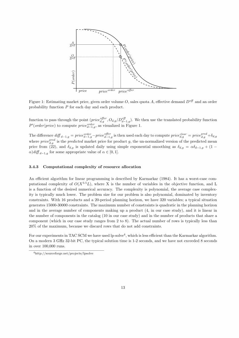
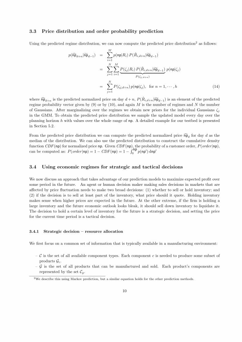
Figure 1: Estimating market price, given order volume O, sales quota A, effective demand Deff and an order

probability function P for each day and each product.

function to pass through the point (priceofferd,g , Od,g/Deffd−1,g). We then use the translated probability function

P ′(order |price) to compute priceorderd−1,g, as visualized in Figure 1.

The difference diff d−1,g = priceorderd−1,g−priceofferd−1,g is then used each day to compute pricecleard,g = pricepredd,g +δd,g

where pricepredd,g is the predicted market price for product g, the un-normalized version of the predicted mean

price from (22), and δd,g is updated daily using simple exponential smoothing as δd,g = αδd−1,g + (1 −α)diff d−1,g for some appropriate value of α ∈ [0, 1].

3.4.3 Computational complexity of resource allocation

An efficient algorithm for linear programming is described by Karmarkar (1984). It has a worst-case com-

putational complexity of O(X3.5L), where X is the number of variables in the objective function, and L

is a function of the desired numerical accuracy. The complexity is polynomial, the average case complex-

ity is typically much lower. The problem size for our problem is also polynomial, dominated by inventory

constraints. With 16 products and a 20-period planning horizon, we have 320 variables; a typical situation

generates 15000-30000 constraints. The maximum number of constraints is quadratic in the planning horizon

and in the average number of components making up a product (4, in our case study), and it is linear in

the number of components in the catalog (10 in our case study) and in the number of products that share a

component (which in our case study ranges from 2 to 8). The actual number of rows is typically less than

20% of the maximum, because we discard rows that do not add constraints.

For our experiments in TAC SCM we have used lp-solve4, which is less efficient than the Karmarkar algorithm.

On a modern 3 GHz 32-bit PC, the typical solution time is 1-2 seconds, and we have not exceeded 8 seconds

in over 100,000 runs.

4http://sourceforge.net/projects/lpsolve

13

4 A case study: The Trading Agent Competition for Supply-

Chain Management (TAC SCM)

We have implemented and tested our approach in an agent-based simulated market environment (Swami-

nathan et al., 1998) in which agents must compete with each other in both procurement and sales markets,

while simultaneously managing inventories, fulfillment, and a manufacturing process. The annual Trading

Agent Competition for Supply Chain Management (TAC SCM) (Collins et al., 2005, 2010b) is a compet-

itive agent-based simulation of an abstract supply chain environment, where software agents make all the

decisions. TAC SCM simulates a market where six autonomous agents compete to maximize profits over

a one-year life cycle for a set of computer models. The simulation takes place over 220 virtual days, each

lasting 15 seconds of real time, of which about 12 seconds can be used for computation and the rest are

needed for communication and simulation server overhead. TAC SCM agents earn money by selling comput-

ers they assemble using parts that they must competitively acquire from suppliers. Each agent has a finite

manufacturing capacity to allocate across a set of products. Each agent must pay to store raw materials

and finished-product inventory, and must borrow money to build its initial inventory. The agent with the

highest bank balance at the end of the simulation wins. TAC SCM is an abstract model of real markets,

leaving out many factors such as quality of products, marketing strategies, long-term procurement contracts,

transportation costs, etc., but has the advantage of enabling a systematic comparison of different strategies

and approaches.

Figure 2: TAC SCM scenario.

Each agent in TAC SCM can produce 16 different types of products, categorized into three market segments

(low, medium, and high quality products). Demand in each market segment varies randomly during the sim-

ulation. Every day each agent receives a set of requests for quotes (RFQs) from several potential customers.

Each customer RFQ specifies the type of product requested, along with quantity, due date, reserve price,

and penalty for late delivery. Each agent may choose to bid on some or all of the day’s RFQs. Customers

accept the lowest bid that is at or below their reserve price, and notify the winning agent. The agent must

ship customer orders on time, or pay a penalty for each day an order is late. Since the environment is

a competitive oligopolistic market, actions of each agent significantly affect the markets, and hence other

agents’ profits and strategies.

14

Organized competitions, such as TAC SCM (Collins et al., 2010b), along with many related computational

tools are driving research into a range of interesting and complex domains that are both socially and eco-

nomically important (Bichler et al., 2010). Since such experimental platforms allow market structures to

be evaluated under a variety of real-world conditions and competitive pressures, they can also be used to

effectively uncover potential hazards of proposed market designs in the face of strategic behaviors on the

part of the participating agents. This can help policy makers in policy and regulation design. For instance,

opportunities for agents to manipulate the TAC SCM competition in unintended ways were uncovered (Ket-

ter et al., 2004), and the simulation model was subsequently updated to more accurately model realistic

supplier behavior.

4.1 Price prediction in TAC SCM

Typical approaches used for price forecasting in TAC SCM are exponential smoothing and linear regression

methods (Benisch et al., 2006; Kontogounis et al., 2006; Jordan et al., 2007; Podobnik et al., 2008). Some

researchers (Zhang et al., 2004) have applied a game theoretic approach to set offer prices, using a variation of

the Cournot game for modeling the product market. Others (He et al., 2006) use fuzzy reasoning to set offer

prices. The TacTex agent predicts the distribution of prices using a weighted average of uniform densities

between the low and high prices from the previous five days, and predicts into the future by assuming that

the distribution of prices does not change (Pardoe and Stone, 2006). The Deep Maize agent uses a variation

of the TacTex algorithm with an additional online update. They employ an online learning procedure that

optimizes predictions according to a logarithmic scoring rule. Deep Maize uses tournament and self-play data

and combines them using an affine transformation (Kiekintveld et al., 2009). They determine the parameters

of the affine transformation by a brute-force search to find values that minimize the scoring rule.

In competitive oligopolistic markets with dynamic pricing, such as TAC SCM, it is also important to model

“order probability” – the probability of winning a customer order at a given price. In TAC SCM, this

probability is typically either estimated by linear interpolation from the minimum and maximum daily

prices (Pardoe and Stone, 2004), or using a linear cumulative density function (CDF) (Benisch et al., 2004)

to estimate the relationship between offer price and order probability, or using a reverse CDF and factors such

as quantity and due date (Ketter et al., 2004). The first two approaches provide a rough approximation of

the real order probability function, the last approach requires the agent to deal with sparse high dimensional

matrices that have to be updated every day during the game. Our approach of economic regimes circumvents

these problems by using only observed market prices and quantities.

5 Evaluation in TAC SCM

We have implemented our approach to drive sales decisions in an agent for the TAC SCM scenario in order

to evaluate its performance. Our experimental agent uses a regime model to compute price distributions

and price trends, and to estimate order probability. Figure 3 shows a schematic view of the major elements

the agent decision processing that leads to making offers at specific prices.

The key elements of this process are the regime model and its training data, described in Section 3, and

the sales quota optimizer, described in Section 3.4.1. The final output is offer prices, computed as described

in Section 3.4.2. Cost basis and inventory status information are derived from a procurement module, and

15

Price

monitor

Median price

estimate

Trend

prediction

Sales

performance

Order Probability

model

Future price

prediction

Demand

prediction

Offer

pricing sales offers

Figure 3: Integrating a regime model into agent sales decision processing. Links connecting the components

affected by the regime model are dashed.

production capacity data is produced by a production scheduling module.

5.1 Real-time regime identification in TAC SCM

In TAC SCM, agents are informed each day of the minimum and maximum order prices for each product on

the previous day, but they cannot observe sales volume or the distribution of prices. As a crude approximation

for the mean price one can use the mid-range normalized price, the price midway between the observed

minimum and maximum. However, since observations of minimum and maximum prices are subject to

noise, some of these observations may be outliers and not representative of the true price distribution.

0 20 40 60 80 100 120 140 160 180 200 220

0.6

0.7

0.8

0.9

1

1.1

1.2

Time in Days

Nor

mal

ized

Pric

e [n

p]

Maximum npMean npMid−Range npSmoothed npMinimum np

0 20 40 60 80 100 120 140 160 180 200 2200

0.2

0.4

0.6

0.8

1

Time in Days

P(R

|np)

EOOBSES

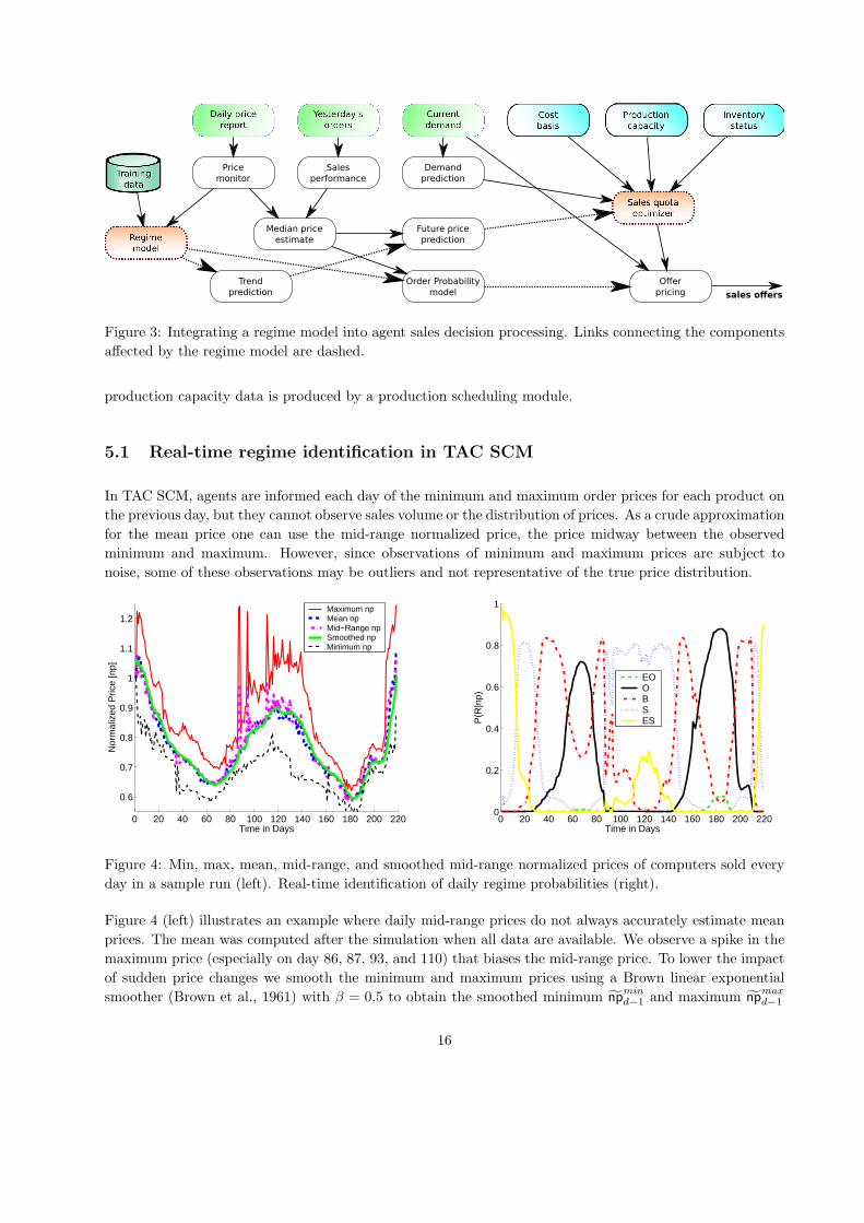
Figure 4: Min, max, mean, mid-range, and smoothed mid-range normalized prices of computers sold every

day in a sample run (left). Real-time identification of daily regime probabilities (right).

Figure 4 (left) illustrates an example where daily mid-range prices do not always accurately estimate mean

prices. The mean was computed after the simulation when all data are available. We observe a spike in the

maximum price (especially on day 86, 87, 93, and 110) that biases the mid-range price. To lower the impact

of sudden price changes we smooth the minimum and maximum prices using a Brown linear exponential

smoother (Brown et al., 1961) with β = 0.5 to obtain the smoothed minimum npmind−1 and maximum np

maxd−1

16

normalized prices, from which we compute the smoothed mid-range normalized price npd−1 as their average.

With a slight abuse of notation in the description of TAC SCM, we use npd for the mid-range price instead

of the mean price.

Figure 4 (right) shows the corresponding regime probabilities computed in real-time during the simulation.

The regimes are indicated as EO (Extreme Oversupply), O (Oversupply), B (Balanced), S (Scarcity), and ES

(Extreme Scarcity). The graph shows that different regimes are dominant at different time points, and that

there are brief intervals during which two regimes are almost equally likely. We have reported a correlation

analysis of the market parameters to regimes and more details on regime identification and other regime

evaluation measures in Ketter et al. (2005); Ketter (2007); Ketter et al. (2009).

5.2 Prediction of price distribution and trend

To obtain a predicted price distribution we sample the price densities defined in (14) every day over the

planning horizon h with values for np between 0 and 1.25, since in TAC SCM reserve prices range up to

125% of nominal component prices. The samples are placed into J = 126 price bins starting from np=0

to np=1.25 in 0.01 increments. Each bin j contains the count of samples with the corresponding price,

np(j) = (j − 1) · 0.01. These counts are then normalized to obtain a probability. For instance, the mean of

the distribution of the predicted normalized prices on day d+ n can be computed as:

E[npd+n] =J∑

j=1

p(npd+n(j) = np(j)|npd−1

)· np(j), for n = 1, · · · , h (22)

To predict price trends we use also the 10%, 50%, and 90% percentile of the predicted price distribution,

which are interpolated from the discretized cumulative distribution.

Figure 5 (left) shows the forecast price density using the repeated 1-day Markov matrix. The dashed curve

represents the price density for the first forecast day, the thick solid line shows the price density for the

last forecast day, and the thin solid curves show the forecast for the intermediate days. As expected, the

predicted price density broadens as we forecast further into the future, reflecting a decreasing certainty in

the prediction. Figure 5 (right) shows the real mean price trend for this example along with forecast price

trends, including the mean Markov prediction, the 10%, 50% and the 90% Markov density percentiles, and

the exponential smoother.

Figure 6 (left) shows the forecast price density based on a n-day Markov prediction for the same simulation

run presented above. We observe that the predicted price density shows significantly less variance as com-

pared to using the repeated 1-day Markov prediction. Figure 6 (right) shows the relative price trend for this

example. The increased certainty in prediction is reflected by the reduced width of the probability envelope,

represented by the 10% and 90% percentile contours. Note that the downward shift in actual prices, Figure 6

(right), is captured by the shift of the predicted future price distribution towards lower prices in Figure 6

(left).

The exponential smoother predictor in this example does not fare well5, since the exponential smoother

puts too much weight on recently observed prices. In this case, prior to the prediction day the prices were

increasing. The exponential smoother predictor takes the recent slope and extrapolates it into the future,

5It is usually better than shown here for near-term predictions, but this example shows one of the advantages of our method.

17

0 0.2 0.4 0.6 0.8 1 1.20

0.005

0.01

0.015

0.02

0.025

0.03

0.035

0.04

0.045

0.05

Normalized Price [np]

Pro

babi

lity

Den

sity

[p(n

p)]

Estimated Density Current Day

115 120 125 130 135−0.25

−0.2

−0.15

−0.1

−0.05

0

0.05

Day [d]

Rel

ativ

e P

rice

Tre

nd

Real PTMean Markov PT10% Markov PT50% Markov PT90% Markov PTExp Smoother PT

Figure 5: Predicted price density (left) and predicted price trend (PT) (right) using the repeated 1-day

Markov matrix for simulation 3717@tac3 from day 115 to day 135.

0 0.2 0.4 0.6 0.8 1 1.20

0.005

0.01

0.015

0.02

0.025

0.03

0.035

0.04

0.045

0.05

Normalized Price [np]

Pro

babi

lity

Den

sity

[p(n

p)]

Estimated Density Current Day

115 120 125 130 135−0.25

−0.2

−0.15

−0.1

−0.05

0

0.05

Day [d]

Rel

ativ

e P

rice

Tre

nd

Real PTMean Markov PT10% Markov PT50% Markov PT90% Markov PTExp Smoother PT

Figure 6: Predicted price density (left) and predicted price trend (PT) (right) using the n-day Markov

prediction for simulation 3717@tac3 from day 115 to day 135.

while our Markov prediction method is able to learn patterns in the data and therefore does much better in

predicting future changes.

5.3 Prediction accuracy

We now demonstrate the accuracy of the predictions made by our method by using it with historical data.

For our experiments, we used data from 28 runs, 18 used for training and 10 for testing (for details please see

the online appendix), played during the semi-finals and finals of TAC SCM 2005. The mix of agents changed

during the simulation runs, with a total of 12 agents in the semi-finals and six in the finals. Since supply

and demand vary in each market segment (low, medium, and high) independently of the other segments, our

18

method is applied independently in each market segment.

5.3.1 Prediction of regime distribution

To determine how well the probability distribution of the predicted regime R matches the one of the actual

regime R, we use the Kullback-Leibler (KL) divergence (Kullback and Leibler, 1951; Kullback, 1959). This

measures the difference between two probability distributions in bits; smaller divergence values correspond

to more accurate predictions. We calculate the KL divergence as:

KL(PR∥PR) =

M∑i=1

PR(ri) log

(PR(ri)

PR(ri)

)(23)

by summing over the regimes ri. The KL divergence can be interpreted in terms of how much additional

data is needed to achieve optimal prediction performance. The precision of this data is given by the number

of bits in the KL-divergence measure. For example a 1 bit difference would require an additional binary

piece of information (Shannon, 1948), like: “Were yesterday’s bids all satisfied?” If the difference between

two distributions is 0 than the predictions are optimal in sense that the predicted and actual distributions

match.

If the time-dependent distribution of a Markov process, in our case PR, converges to a limit, Π = limm→∞ {PR}mthen Π is called the stationary distribution. When the stationary distribution exists it is characterized by

the fix-point equation Π = Tn · Π. There are several ways to compute the stationary distribution, Π,

which involve solving the eigenvalue problem specified in the above equation (for details consult the online

appendix).

We introduced the n-day Markov matrix because we hypothesized that the n-day Markov matrix will take

longer to reach the stationary distribution of its Markov process than the 1-day Markov matrix, and therefore

it will deliver a better prediction performance. We prove this hypothesis empirically by calculating the

stationary distribution Π for the 1-day and each n-day Markov matrices and comparing it with the Markov

predicted regime distribution, using again the KL-divergence between P (R) and Π.

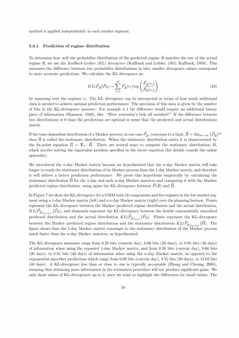
In Figure 7 we show the KL-divergence for a GMMwith 16 components and five regimes in the low market seg-

ment using a 1-day Markov matrix (left) and a n-day Markov matrix (right) over the planning horizon. Points

represent the KL-divergence between the Markov predicted regime distribution and the actual distribution,

KL(PRMarkov∥PR), and diamonds represent the KL-divergence between the double exponentially smoothed

predicted distribution and the actual distribution KL(PRExpS∥PR). Pluses represent the KL-divergence

between the Markov predicted regime distribution and the stationary distribution KL(PRMarkov∥Π). The

figure shows that the 1-day Markov matrix converges to the stationary distribution of the Markov process

much faster than the n-day Markov matrices, as hypothesized.

The KL-divergence measures range from 0.28 bits (current day), 0.80 bits (20 days), to 0.95 bits (40 days)

of information when using the repeated 1-day Markov matrix, and from 0.28 bits (current day), 0.66 bits

(20 days), to 0.81 bits (40 days) of information when using the n-day Markov matrix, as opposed to the

exponential smoother predictions which range from 0.09 bits (current day), 3.55 bits (20 days), to 12.62 bits

(40 days). A KL-divergence less than or close to one is typically acceptable (Zhang and Cheung, 2005),

meaning that obtaining more information in the estimation procedure will not produce significant gains. We

only show values of KL-divergences up to 4, since we want to highlight the differences for small values. The

19

0 5 10 15 20 25 30 35 400

0.5

1

1.5

2

2.5

3

3.5

4

Planning Horizon [Day]

KL−

Div

erge

nce

KLPred_Actual_Markov

KLPred_Actual_ExpS

KLPred_Stat_Markov

0 5 10 15 20 25 30 35 400

0.5

1

1.5

2

2.5

3

3.5

4

Planning Horizon [Day]

KL−

Div

erge

nce

KLPred_Actual_Markov

KLPred_Actual_ExpS

KLPred_Stat_Markov

Figure 7: KL-divergence between predicted, actual, and stationary regime distribution using a repeated

1-day (left) vs n-day (right) Markov matrix, computed using five regimes on a GMM with 16 components

for the low market segment over the testing set.

current day exponential smoother predictions are approximately 1.14 times better than the repeated 1-day

and n-day Markov predictions. On the other hand at 20 and 40 days, the exponential smoother predictions

are approximately 6.73 and 3259 times worse than the repeated 1-day Markov predictions and 7.42 and 3591

times worse than the n-day Markov predictions.

The KL-divergence values calculated using the n-day Markov matrix are always smaller than the repeated

1-day Markov matrix, significantly so in the long-term. This indicates a better fit between the predicted and

the actual regime probabilities for the n-day Markov matrix. As a consequence the n-day Markov matrix

should be used instead of the repeated 1-day Markov matrix for strategic decision making. The best estimate

for the short-term (current day up to 4 days into the future) is given by the exponential smoother, which

should be used to generate price densities for the short-term and sales offer prices for the current day, i.e.

for tactical decision making.

5.3.2 Comparison of price prediction methods

We compute the price density, p(npd+n)6, for the next n days into the future, where p(npd) is the distribution

of normalized prices on day d. We calculated the expected mean price using (22), and tracked different

contours (10%, 50%, and 90%) of the price density curve. We calculated the root mean square error,

RMSE (npn, npn), between the predicted normalized prices, npn, and the actual normalized price, npn, over

a prediction interval of n days in the planning horizon h, averaged across days and runs, to determine the

accuracy of the price prediction as:

RMSE ( npn, npn) =

√√√√√NG∑i=1

ND−n∑d=1

( npn,id − npn,id

)2NG · (ND − n)

, for n = 1, · · · , h (24)

6For simplicity of notation here we leave out the dependence on historical normalized prices.

20

where ND is the number of days in a TAC SCM simulation, NG is the number of simulation runs, and npn,i

d

is the predicted price vector for run i for n days into the future. In our experiments we chose an horizon

h = 40.

For these experiments we calculated the expected mean price using our three prediction methods, i.e. the

exponential smoother with regimes (Section 3.2.2), the Markov prediction (Section 3.2.3), and the Markov

correction-prediction (Section 3.2.4) methods.

We have also implemented three different comparison baselines, using approaches taken by successful TAC

SCM agents.

1. The first baseline is an exponential smoother prediction, which is widely used as a baseline (Wang

et al., 2008). In TAC SCM exponential smoothing and linear regression methods are also commonly

used for price forecasting (Benisch et al., 2006; Kontogounis et al., 2006; Jordan et al., 2007; Podobnik

et al., 2008).

2. The second is a constant predictor used by the Botticelli agent, which estimates the current mean

price using least-squares linear regression fitting yesterday minimum and maximum prices and its own

average offer prices against the ratio of the number of offers won to the number of offers issued, and

uses this value until the end of the planning horizon (Benisch et al., 2004).

3. As a third baseline we implemented the heuristic predictor used by TacTex, the most successful agent of

the TAC SCM tournament (Pardoe and Stone, 2006). This baseline method predicts the distribution of

prices using a weighted average of uniform densities between the low and high prices from the previous

five days. We use weights of 0.3 for the two most recent days, 0.2 for the middle day, and 0.1 for the

two oldest days. We predict this into the future by assuming that the distribution of prices does not

change. We consider this our main baseline, because it uses an information constraint in the current

price level, and relies completely on local price stability for predictive power. It was also used as a

benchmark by the Deep Maize team to test their predictions (Kiekintveld et al., 2009).

0 5 10 15 20 25 30 35 400

0.05

0.1

0.15

0.2

0.25

Planning Horizon [Day]

RM

S P

rice

Pre

dict

ion

Err

or

Median Markov C−PMedian Markov PMedian Exp Smoother RegimesExp SmootherBotticelliTacTex

0 5 10 15 20 25 30 35 400

0.05

0.1

0.15

0.2

0.25

Planning Horizon [Day]

RM

S P

rice

Pre

dict

ion

Err

or

Median Markov C−PMedian Markov PMedian Exp Smoother RegimesExp SmootherBotticelliTacTex

Figure 8: RMS error for price prediction based on a repeated 1-day (left) vs n-day (right) Markov matrix.

Three regime-based prediction methods are compared to three baseline methods, exponential smoothing and

methods used by other successful TAC SCM agents.

21

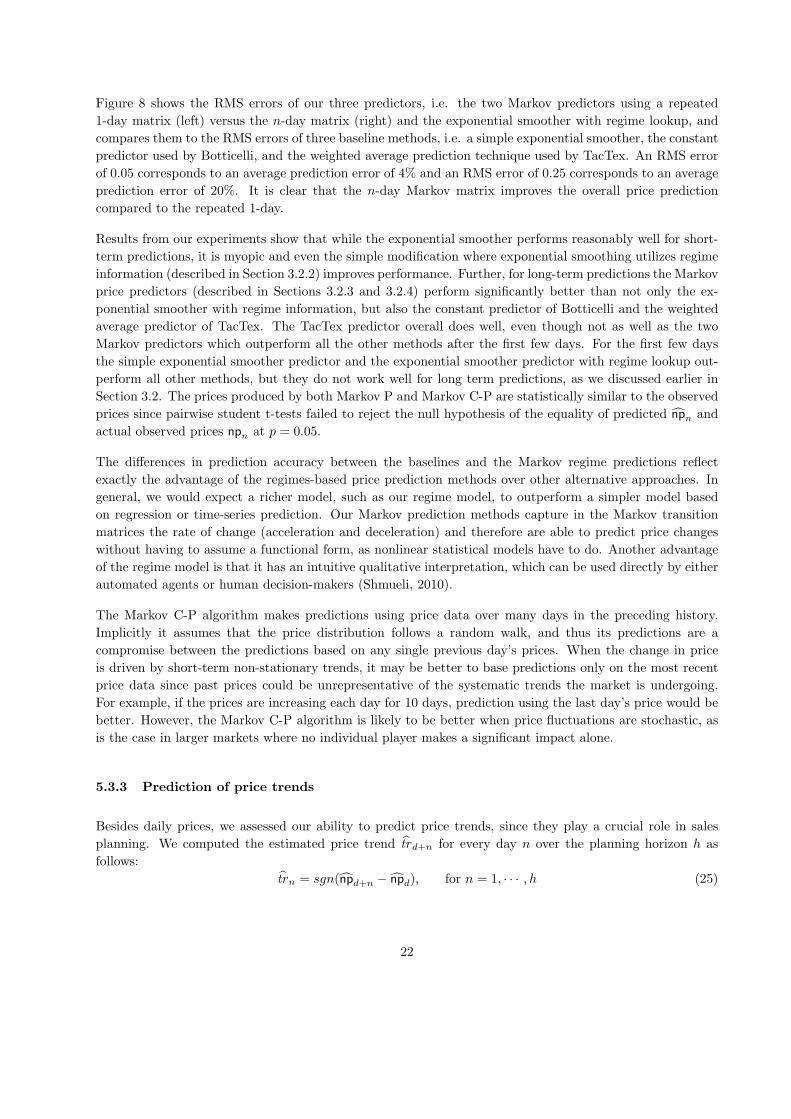
Figure 8 shows the RMS errors of our three predictors, i.e. the two Markov predictors using a repeated

1-day matrix (left) versus the n-day matrix (right) and the exponential smoother with regime lookup, and

compares them to the RMS errors of three baseline methods, i.e. a simple exponential smoother, the constant

predictor used by Botticelli, and the weighted average prediction technique used by TacTex. An RMS error

of 0.05 corresponds to an average prediction error of 4% and an RMS error of 0.25 corresponds to an average

prediction error of 20%. It is clear that the n-day Markov matrix improves the overall price prediction

compared to the repeated 1-day.

Results from our experiments show that while the exponential smoother performs reasonably well for short-

term predictions, it is myopic and even the simple modification where exponential smoothing utilizes regime

information (described in Section 3.2.2) improves performance. Further, for long-term predictions the Markov

price predictors (described in Sections 3.2.3 and 3.2.4) perform significantly better than not only the ex-

ponential smoother with regime information, but also the constant predictor of Botticelli and the weighted

average predictor of TacTex. The TacTex predictor overall does well, even though not as well as the two

Markov predictors which outperform all the other methods after the first few days. For the first few days

the simple exponential smoother predictor and the exponential smoother predictor with regime lookup out-

perform all other methods, but they do not work well for long term predictions, as we discussed earlier in

Section 3.2. The prices produced by both Markov P and Markov C-P are statistically similar to the observed

prices since pairwise student t-tests failed to reject the null hypothesis of the equality of predicted npn and

actual observed prices npn at p = 0.05.

The differences in prediction accuracy between the baselines and the Markov regime predictions reflect

exactly the advantage of the regimes-based price prediction methods over other alternative approaches. In

general, we would expect a richer model, such as our regime model, to outperform a simpler model based

on regression or time-series prediction. Our Markov prediction methods capture in the Markov transition

matrices the rate of change (acceleration and deceleration) and therefore are able to predict price changes

without having to assume a functional form, as nonlinear statistical models have to do. Another advantage

of the regime model is that it has an intuitive qualitative interpretation, which can be used directly by either

automated agents or human decision-makers (Shmueli, 2010).

The Markov C-P algorithm makes predictions using price data over many days in the preceding history.

Implicitly it assumes that the price distribution follows a random walk, and thus its predictions are a

compromise between the predictions based on any single previous day’s prices. When the change in price

is driven by short-term non-stationary trends, it may be better to base predictions only on the most recent

price data since past prices could be unrepresentative of the systematic trends the market is undergoing.

For example, if the prices are increasing each day for 10 days, prediction using the last day’s price would be

better. However, the Markov C-P algorithm is likely to be better when price fluctuations are stochastic, as

is the case in larger markets where no individual player makes a significant impact alone.

5.3.3 Prediction of price trends

Besides daily prices, we assessed our ability to predict price trends, since they play a crucial role in sales

planning. We computed the estimated price trend trd+n for every day n over the planning horizon h as

follows:

trn = sgn(npd+n − npd), for n = 1, · · · , h (25)

22

where sgn is the sign function, and npd and npd+n are the predicted prices respectively on day d and day

d+ n. Since the agent has access only to the minimum and maximum prices of the previous day, it needs a

one day forecast of the mid range price to estimate the price on the current day d. If trn is positive, then

the predicted prices are increasing, otherwise they are decreasing.

Figure 9 displays the success rate of price trend sign prediction using a repeated 1-day Markov matrix (left)

and a n-day Markov matrix (right). Since the price trend is used for strategic decision making, we calculated

the success rate starting at d+5. As the figure demonstrates, the Markov correction-prediction predicted the

correct trend about 70% of time and dominated the exponential smoothing approach. In general, the n-day

Markov predictions performed better than the repeated 1-day Markov matrix. In the figure we show the

success rate using the expected means of the distributions, computed using Eq. 22, as well as the medians

of the distributions.

5 10 15 20 25 30 35 4050

55

60

65

70

75

Planning Horizon [Day]

Tre

nd S

ucce

ss R

ate

in %

Expected Mean Markov C−PExpected Mean Markov PMedian Markov C−PMedian Markov PExp Smoother

5 10 15 20 25 30 35 4050

55

60

65

70

75

Planning Horizon [Day]

Tre

nd S

ucce

ss R

ate

in %

Expected Mean Markov C−PExpected Mean Markov PMedian Markov C−PMedian Markov PExp Smoother

Figure 9: Success rate of price trend predictions based on 1-day (left) vs. n-day (right) Markov matrix.

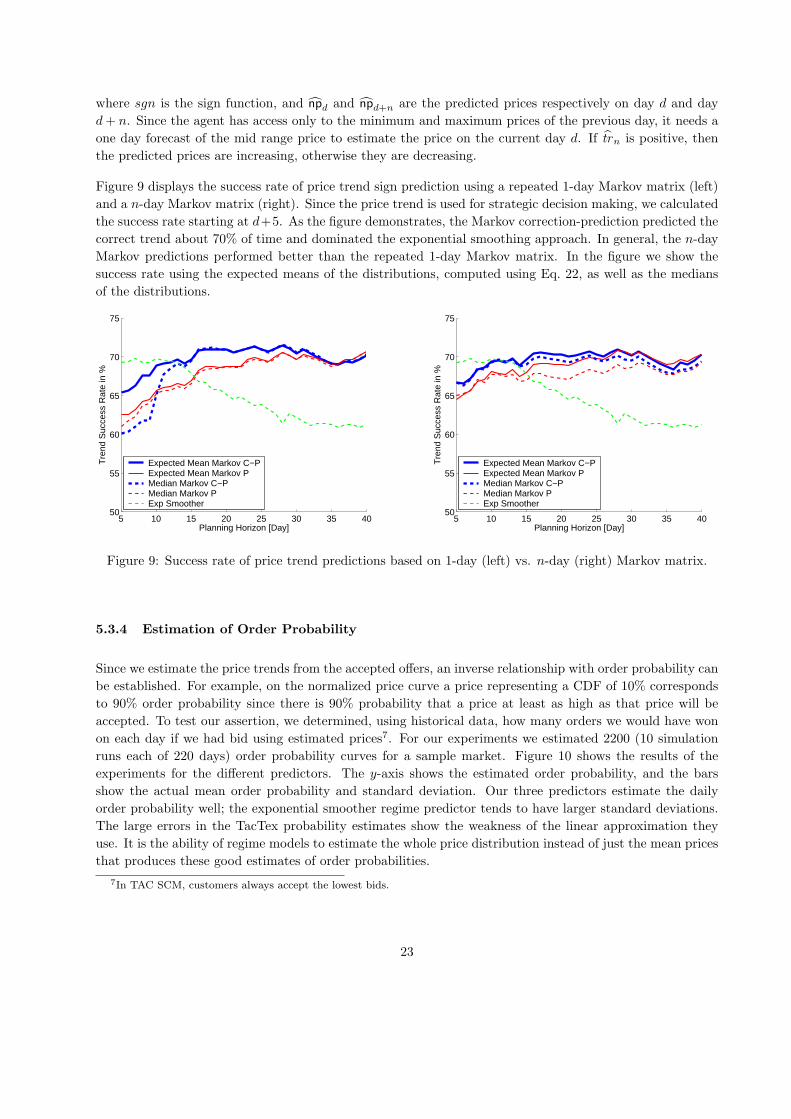
5.3.4 Estimation of Order Probability

Since we estimate the price trends from the accepted offers, an inverse relationship with order probability can

be established. For example, on the normalized price curve a price representing a CDF of 10% corresponds

to 90% order probability since there is 90% probability that a price at least as high as that price will be

accepted. To test our assertion, we determined, using historical data, how many orders we would have won

on each day if we had bid using estimated prices7. For our experiments we estimated 2200 (10 simulation

runs each of 220 days) order probability curves for a sample market. Figure 10 shows the results of the

experiments for the different predictors. The y-axis shows the estimated order probability, and the bars

show the actual mean order probability and standard deviation. Our three predictors estimate the daily

order probability well; the exponential smoother regime predictor tends to have larger standard deviations.

The large errors in the TacTex probability estimates show the weakness of the linear approximation they

use. It is the ability of regime models to estimate the whole price distribution instead of just the mean prices

that produces these good estimates of order probabilities.

7In TAC SCM, customers always accept the lowest bids.

23

np(10%) np(25%) np(50%) np(75%) np(90%)

10%

25%

50%

75%

90%

Normalized Price by Density Percentile

Est

imat

ed O

rder

Pro

babi

lity

with

Err

orba

rs

Markov C−PMarkov PExp Smoother RegimesTacTex

Figure 10: Daily order probability estimation (mean/std) for the 10th, 25th, 50th, 75th, and 90th percentile

using different predictors.

5.4 Agent performance

The analysis presented so far demonstrates that our approach performs well with historical data. However,

to make decisions in real time, the methods have to be dynamic and self-adjusting. We next evaluate the

performance of our approach when used by an agent that plays against five other agents in real-time in TAC

SCM.

5.4.1 Experimental setup

We implemented different prediction methods for short term (tactical) and long-term (strategic) predictions

and tested them in real-time in our MinneTAC (?Collins et al. (2010a)) agent. The prediction methods

we tested are: linear predictor, exponential smoother, exponential smoother with regimes, Markov 1-day

predictor, and Markov n-day predictor.

The agents we used for our experiments have been obtained from the TAC SCM agent repository8. We

selected five of the finalists from the 2006 competition and an agent from the 2005 competition. The agents

are: (1) TacTex, from the University of Texas at Austin; (2) DeepMaize, from the University of Michigan; (3)

PhantAgent, from the Politechnica University of Bucharest; (4) Maxon, from Xonar Inc; (5) RationalSCM,

from the Australian National University; and (6) “our agent”.

Agent performance in TAC SCM is affected not only by the set of competing agents, but also by random

variations in supply, demand, and other market parameters. To compare different variations of our own

agent without having to run a very large number of simulation runs, we used a version of the simulation

server (Sodomka et al., 2007) that supports repeatable pseudo-random sequences of any individual market

8http://www.sics.se/tac/showagents.php

24

factor or combination of factors. The use of this server removes the profit variability due to agents facing

different market conditions and enables us to test multiple variations of our agent under repeatable market

conditions.

We ran NG = 23 simulations, each with a different pseudo-random sequence, using the base version of

MinneTAC, and then ran NG simulations with the same market factors each using a different version

of MinneTAC with different prediction models for tactical (order probability calculation when responding

to RFQs) and strategic decisions (price and price trend prediction for sales quota and inventory holding

decisions). At the strategic level we used different price prediction methods, namely an exponential smoother,

an exponential smoother with regimes, a Markov prediction process with 1-day, and a Markov prediction

process with n-day predictions. At the tactical level we used two methods to calculate order probability,

one based on a linear interpolation between the estimated minimum and maximum daily prices, the other

an exponential smoother with economic regimes.

The design of the simulation limits agents to about 12 seconds for each daily decision cycle, which must

be allocated among procurement, manufacturing, and sales processes. The linear program described in

Section 3.4.1 requires up to 8 seconds to complete. All of the regime models described in this paper are able

to produce results in less than one second on modern desktop machines.

5.4.2 Real-time results

Our tests included five sets of 23 simulations each, one set for each different configuration of our agent, using

the same 23 pseudo-random sequences for each set.

As the primary measure of agent performance in Table 1 we show the mean total profit per agent. Table 1

shows that our agent always comes in fifth when competing against this set of agents. The performance of

an agent depends upon its entire decision processes, which cover procurement, manufacturing and sales. Our

agent is somewhat weaker than its competitors in the procurement and manufacturing areas, but since our

work is focused on sales performance, we are only interested in the relative performance of our agent under

different sales strategies. The results of the experiments are as follows:

1. In the first experiment our agent used a linear interpolation to determine the probability of order and

an exponential smoother to predict price trends. The final mean profit is 1.347 million.

2. In the second experiment our agent used again a linear interpolation to determine the probability of

order, and economic regimes (based on a repeated 1-day Markov prediction) to predict price trends.

The final mean profit was 1.813 million.

3. The third experiment used an exponential smoother with regimes both to predict prices and to de-

termine the order probability, median prices and price trends. It had a final mean profit of 1.545

million.

4. The fourth experiment used an exponential smoother with regimes for tactical decisions (determination

of order probability) and a repeated 1-day Markov predictor for strategic decisions (price and price

trend prediction). The final mean profit for this experiment was 2.117 million, the best among the

tested configurations.

5. The fifth experiment used an exponential smoother with regimes for tactical decisions and a Markov

n-day prediction to determine price trends. Its final mean profit was 1.567 million.

25

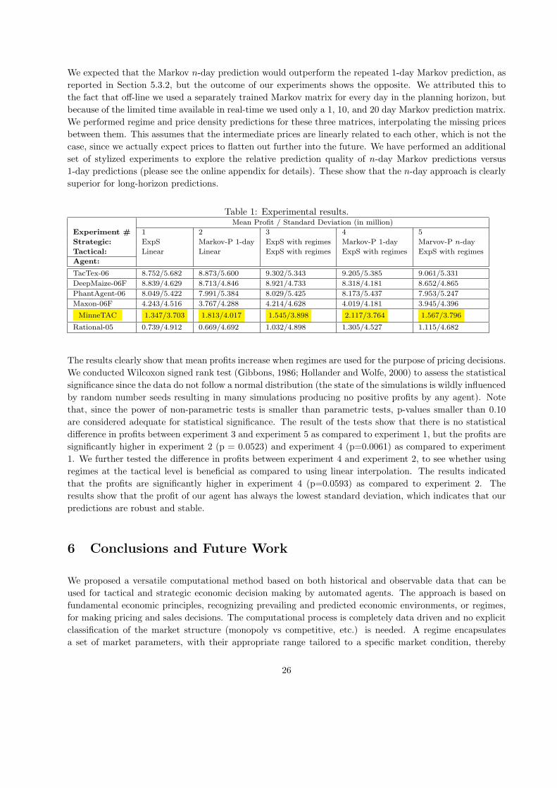
We expected that the Markov n-day prediction would outperform the repeated 1-day Markov prediction, as

reported in Section 5.3.2, but the outcome of our experiments shows the opposite. We attributed this to

the fact that off-line we used a separately trained Markov matrix for every day in the planning horizon, but

because of the limited time available in real-time we used only a 1, 10, and 20 day Markov prediction matrix.

We performed regime and price density predictions for these three matrices, interpolating the missing prices

between them. This assumes that the intermediate prices are linearly related to each other, which is not the

case, since we actually expect prices to flatten out further into the future. We have performed an additional

set of stylized experiments to explore the relative prediction quality of n-day Markov predictions versus

1-day predictions (please see the online appendix for details). These show that the n-day approach is clearly

superior for long-horizon predictions.

Table 1: Experimental results.Mean Profit / Standard Deviation (in million)

Experiment # 1 2 3 4 5

Strategic: ExpS Markov-P 1-day ExpS with regimes Markov-P 1-day Marvov-P n-day

Tactical: Linear Linear ExpS with regimes ExpS with regimes ExpS with regimes

Agent:

TacTex-06 8.752/5.682 8.873/5.600 9.302/5.343 9.205/5.385 9.061/5.331

DeepMaize-06F 8.839/4.629 8.713/4.846 8.921/4.733 8.318/4.181 8.652/4.865

PhantAgent-06 8.049/5.422 7.991/5.384 8.029/5.425 8.173/5.437 7.953/5.247

Maxon-06F 4.243/4.516 3.767/4.288 4.214/4.628 4.019/4.181 3.945/4.396

MinneTAC 1.347/3.703 1.813/4.017 1.545/3.898 2.117/3.764 1.567/3.796

Rational-05 0.739/4.912 0.669/4.692 1.032/4.898 1.305/4.527 1.115/4.682

The results clearly show that mean profits increase when regimes are used for the purpose of pricing decisions.

We conducted Wilcoxon signed rank test (Gibbons, 1986; Hollander and Wolfe, 2000) to assess the statistical

significance since the data do not follow a normal distribution (the state of the simulations is wildly influenced

by random number seeds resulting in many simulations producing no positive profits by any agent). Note

that, since the power of non-parametric tests is smaller than parametric tests, p-values smaller than 0.10

are considered adequate for statistical significance. The result of the tests show that there is no statistical

difference in profits between experiment 3 and experiment 5 as compared to experiment 1, but the profits are

significantly higher in experiment 2 (p = 0.0523) and experiment 4 (p=0.0061) as compared to experiment

1. We further tested the difference in profits between experiment 4 and experiment 2, to see whether using

regimes at the tactical level is beneficial as compared to using linear interpolation. The results indicated

that the profits are significantly higher in experiment 4 (p=0.0593) as compared to experiment 2. The

results show that the profit of our agent has always the lowest standard deviation, which indicates that our

predictions are robust and stable.

6 Conclusions and Future Work

We proposed a versatile computational method based on both historical and observable data that can be

used for tactical and strategic economic decision making by automated agents. The approach is based on

fundamental economic principles, recognizing prevailing and predicted economic environments, or regimes,

for making pricing and sales decisions. The computational process is completely data driven and no explicit

classification of the market structure (monopoly vs competitive, etc.) is needed. A regime encapsulates

a set of market parameters, with their appropriate range tailored to a specific market condition, thereby

26

reducing the dimensionality of the parameter space. This results in a fast computational approach. Economic

regimes provide comparatively more degrees of freedom than ordinary regression based approaches, since the

full price distribution is available for decision making. Availability of complete distributions and their

trends allows a decision maker to choose an appropriate level of risk, and supports estimation of other

useful metrics such as order probabilities. Economic regimes are especially suited to make predictions in

non stationary environments where supply-demand relationship is highly dynamic. Economic regimes also

provide an opportunity for niche learning, i.e., an agent is able to apply different approaches and actions

when specific regimes are dominant.

We presented three different algorithms for dynamic identification of regimes and for prediction of regime

distribution over a planning horizon. Our methods use knowledge of current and future regime distributions

to facilitate tactical decision making, such as calculation of customer offer prices, and strategic decision

making, such as allocation of resources over a planning horizon. Using the complete price distribution,

instead of point estimates of prices, enables our approach to better account for price variance in decision

making. Our choice of using only price and its associated quantity information to estimate regimes makes our

approach applicable in real world competitive environments. In a real world market environment companies

are able to observe competitors prices, but have no access to internal data, such as costs, manufacturing

capacity, and inventory positions.

In future, we intend to apply our method in other domains where predicting price distributions may be

fruitful, including B2B domains such as computer chips and components, B2C domains such as Amazon.com,

and eBay.com, and in financial applications.

A real B2B domain we are currently working with is the Dutch Flower Auctions (DFA) (Kambil and van

Heck, 1998). We have established a cooperation with the DFA and begun work to apply economic regimes

to the flower market. The DFA play a vital role in maintaining the Netherlands’s leadership in the flower

industry; they serve as efficient centers for flower exchange between suppliers and buyers. In 2009, the DFA

reported daily trades of over 37.0 million cut flowers and 2.6 million potted plants, generating over 3.81

billion Euros in annual sales.

In the DFA, bidders decide which and how many flowers to bid on and at what price, while the auctioneers

set initial prices, reserve prices, minimum lot sizes, and clock speeds. In the current practice, those auc-

tioneering parameters are set up in a static manner. Realizing the opportunities offered by dynamic pricing

in maximizing revenue (Zhao and Zheng, 2000), and in order to increase the auction efficiency, we propose

to move the auctioneer away from the current practice of static starting price setup to dynamic pricing

using our method of economic regimes. Bidders could also use economic regimes to predict different market

regimes and associated prices, and align all elements of the supply-chain accordingly, especially procurement

and sales. An opportunistic buyer might bid low for certain flowers in an over-supply situation, since he

could sell them up to some threshold at a profit. On the other hand, if a scarcity situation is predicted, then

the buyer might start bidding for certain flowers a few days earlier and store them in cold storage until the

price reaches the highest point, e.g. mother’s day.

27

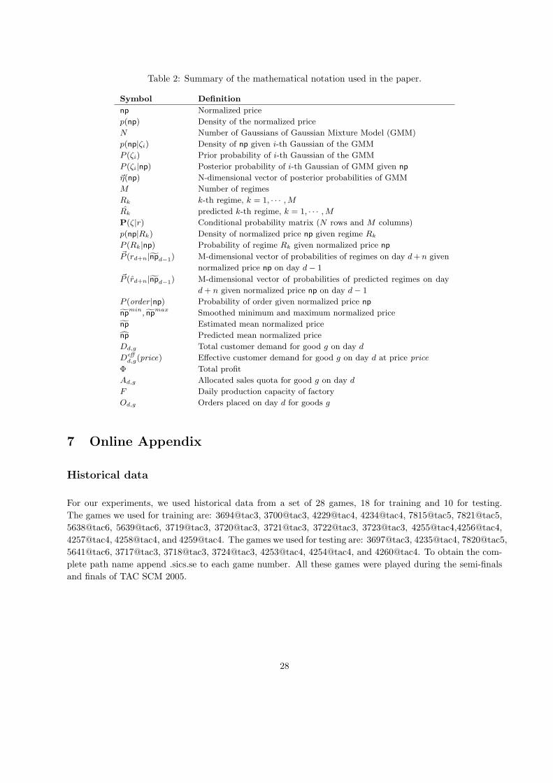
Table 2: Summary of the mathematical notation used in the paper.

Symbol Definition

np Normalized price

p(np) Density of the normalized price

N Number of Gaussians of Gaussian Mixture Model (GMM)

p(np|ζi) Density of np given i-th Gaussian of the GMM

P (ζi) Prior probability of i-th Gaussian of the GMM

P (ζi|np) Posterior probability of i-th Gaussian of GMM given np

η(np) N-dimensional vector of posterior probabilities of GMM

M Number of regimes

Rk k-th regime, k = 1, · · · ,MRk predicted k-th regime, k = 1, · · · ,MP(ζ|r) Conditional probability matrix (N rows and M columns)

p(np|Rk) Density of normalized price np given regime Rk

P (Rk|np) Probability of regime Rk given normalized price np

P (rd+n|npd−1) M-dimensional vector of probabilities of regimes on day d+n given

normalized price np on day d− 1

P (rd+n|npd−1) M-dimensional vector of probabilities of predicted regimes on day

d+ n given normalized price np on day d− 1

P (order |np) Probability of order given normalized price np

npmin, npmax Smoothed minimum and maximum normalized price

np Estimated mean normalized price

np Predicted mean normalized price

Dd,g Total customer demand for good g on day d

Deffd,g(price) Effective customer demand for good g on day d at price price

Φ Total profit

Ad,g Allocated sales quota for good g on day d

F Daily production capacity of factory

Od,g Orders placed on day d for goods g

7 Online Appendix

Historical data

For our experiments, we used historical data from a set of 28 games, 18 for training and 10 for testing.

The games we used for training are: 3694@tac3, 3700@tac3, 4229@tac4, 4234@tac4, 7815@tac5, 7821@tac5,

5638@tac6, 5639@tac6, 3719@tac3, 3720@tac3, 3721@tac3, 3722@tac3, 3723@tac3, 4255@tac4,4256@tac4,

4257@tac4, 4258@tac4, and 4259@tac4. The games we used for testing are: 3697@tac3, 4235@tac4, 7820@tac5,

5641@tac6, 3717@tac3, 3718@tac3, 3724@tac3, 4253@tac4, 4254@tac4, and 4260@tac4. To obtain the com-

plete path name append .sics.se to each game number. All these games were played during the semi-finals

and finals of TAC SCM 2005.

28

Reasons for selecting a Gaussian Mixture Model

We use a GMM since it is able to approximate arbitrary density functions. Another advantage is that

the GMM is a semi-parametric approach which can be computed fast and uses less memory than other

approaches. The GMM is one way of modeling a probability density function p(x), given a finite number of

data points Xs, s = 1, . . . , S drawn from that density.

We decided to use this model over other possible models for various reasons. First, there are three alter-

natives to approach the density estimation problem: parametric, non-parametric, and semi-parametric. In

parametric methods one assumes a specific functional form for the density model. Its parameters are then

optimized by fitting the model to the data set. For instance, the functional form can be a Gaussian and the

parameters the mean µ and standard deviation σ of that distribution. The drawback is that the functional

form might not be consistent with the data and may result in unsatisfactory estimation.

In non-parametric estimation methods the form of the density is determined entirely by the data, i.e. no

particular functional form is assumed, e.g., histograms, kernel-based methods, K-nearest-neighbors and

Parzen window (Bishop, 1995; Duda et al., 2000; Nabney, 2001). The drawback is that huge data sets are

needed for good models and that parameter tuning is critical for performance.

In semi-parametric estimation methods a general class of functional forms is allowed and the number of

adaptive parameters can be adapted in a systematic way allowing even more flexible models, e.g. more

hidden units, multi-layer perceptrons, radial basis functions and Gaussian mixture models. The advantage

is that these methods combine the best characteristics of parametric and non-parametric methods. The

complexity of the model increases only with the total number of parameters in the model, and not with the

size of the data set.

The demand characteristics in electronic marketplaces have been found to be fractal, that is the short-term

demand pattern has much larger variation than the long-term time-averaged demand pattern (Gupta et al.,

1997). This means that while there are periods of no or little demand there will be periods when demand

will be extremely high. The pricing strategy of an agent needs to take this into account. Traditionally

parameterized econometric models perform poorly in these situations. On the contrary, non-parametric

approaches do an excellent job in estimation, but are usually computationally too expensive. In the TAC

SCM domain, our testbed, and in many real-world trading scenarios decisions have to be made fast and there

is not enough time for time consuming computations. Therefore, we selected a semi-parametric approach,

and in particular the GMM.

Determination of the optimal number of Gaussians for the GMM

We developed an algorithm (see Figure 11) to find the optimal number of Gaussians in the GMM. The

algorithm iterates from 1 to N Gaussian components and for each set of Gaussians it fits a GMM to all the

historical normalized price data from the training set. New normalized price samples are generated from

each fitted GMM model via Monte-Carlo sampling, with the number of new samples matching the original

data size. Price histograms are generated using the same bins for the original and sampled data, and are

compared with the help of the KL-divergence (Kullback and Leibler (1951); Kullback (1959))9. For each set

9With the KL-divergence we are able to measure the closeness of two distributions. If the two distributions are exactly the

same, then the KL-divergence is zero. A more detailed discussion of the KL-divergence can be found in (citation suppressed

29

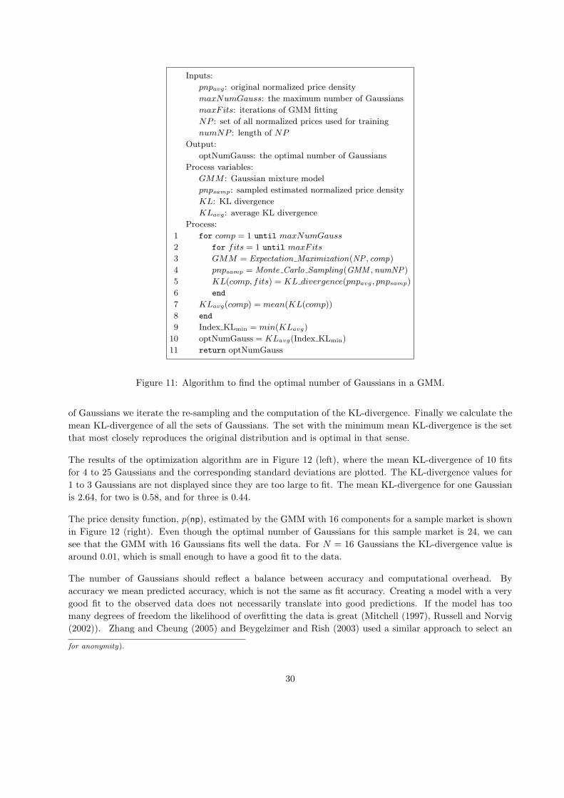
Inputs:

pnpavg: original normalized price density

maxNumGauss: the maximum number of Gaussians

maxFits: iterations of GMM fitting

NP : set of all normalized prices used for training

numNP : length of NP

Output:

optNumGauss: the optimal number of Gaussians

Process variables:

GMM : Gaussian mixture model

pnpsamp: sampled estimated normalized price density

KL: KL divergence

KLavg: average KL divergence

Process:

1 for comp = 1 until maxNumGauss

2 for fits = 1 until maxFits

3 GMM = Expectation Maximization(NP , comp)

4 pnpsamp = Monte Carlo Sampling(GMM ,numNP)

5 KL(comp, fits) = KL divergence(pnpavg, pnpsamp)

6 end

7 KLavg(comp) = mean(KL(comp))

8 end

9 Index KLmin = min(KLavg)

10 optNumGauss = KLavg(Index KLmin)

11 return optNumGauss

Figure 11: Algorithm to find the optimal number of Gaussians in a GMM.

of Gaussians we iterate the re-sampling and the computation of the KL-divergence. Finally we calculate the

mean KL-divergence of all the sets of Gaussians. The set with the minimum mean KL-divergence is the set

that most closely reproduces the original distribution and is optimal in that sense.

The results of the optimization algorithm are in Figure 12 (left), where the mean KL-divergence of 10 fits

for 4 to 25 Gaussians and the corresponding standard deviations are plotted. The KL-divergence values for

1 to 3 Gaussians are not displayed since they are too large to fit. The mean KL-divergence for one Gaussian

is 2.64, for two is 0.58, and for three is 0.44.

The price density function, p(np), estimated by the GMM with 16 components for a sample market is shown

in Figure 12 (right). Even though the optimal number of Gaussians for this sample market is 24, we can

see that the GMM with 16 Gaussians fits well the data. For N = 16 Gaussians the KL-divergence value is

around 0.01, which is small enough to have a good fit to the data.

The number of Gaussians should reflect a balance between accuracy and computational overhead. By

accuracy we mean predicted accuracy, which is not the same as fit accuracy. Creating a model with a very

good fit to the observed data does not necessarily translate into good predictions. If the model has too

many degrees of freedom the likelihood of overfitting the data is great (Mitchell (1997), Russell and Norvig

(2002)). Zhang and Cheung (2005) and Beygelzimer and Rish (2003) used a similar approach to select an

for anonymity).

30

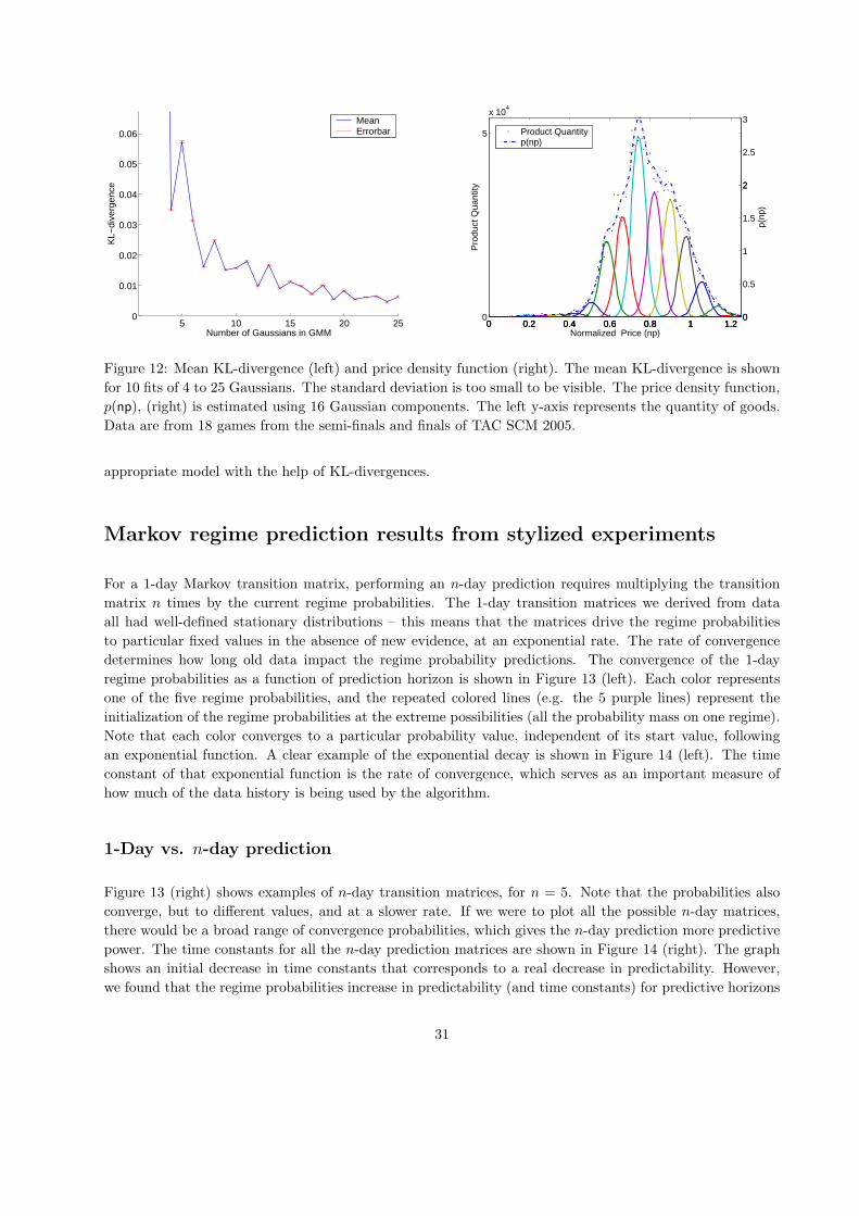
5 10 15 20 250

0.01

0.02

0.03

0.04

0.05

0.06

Number of Gaussians in GMM

KL−

dive

rgen

ceMeanErrorbar

0 0.2 0.4 0.6 0.8 1 1.20

5

x 104

Pro

duct

Qua

ntity

Normalized Price (np)0 0.2 0.4 0.6 0.8 1 1.2

0

0.5

1

1.5

2

2.5

3

p(np

)

0 0.2 0.4 0.6 0.8 1 1.20

2

Product Quantityp(np)

Figure 12: Mean KL-divergence (left) and price density function (right). The mean KL-divergence is shown

for 10 fits of 4 to 25 Gaussians. The standard deviation is too small to be visible. The price density function,

p(np), (right) is estimated using 16 Gaussian components. The left y-axis represents the quantity of goods.

Data are from 18 games from the semi-finals and finals of TAC SCM 2005.

appropriate model with the help of KL-divergences.

Markov regime prediction results from stylized experiments

For a 1-day Markov transition matrix, performing an n-day prediction requires multiplying the transition

matrix n times by the current regime probabilities. The 1-day transition matrices we derived from data

all had well-defined stationary distributions – this means that the matrices drive the regime probabilities

to particular fixed values in the absence of new evidence, at an exponential rate. The rate of convergence

determines how long old data impact the regime probability predictions. The convergence of the 1-day

regime probabilities as a function of prediction horizon is shown in Figure 13 (left). Each color represents

one of the five regime probabilities, and the repeated colored lines (e.g. the 5 purple lines) represent the

initialization of the regime probabilities at the extreme possibilities (all the probability mass on one regime).

Note that each color converges to a particular probability value, independent of its start value, following

an exponential function. A clear example of the exponential decay is shown in Figure 14 (left). The time

constant of that exponential function is the rate of convergence, which serves as an important measure of

how much of the data history is being used by the algorithm.

1-Day vs. n-day prediction

Figure 13 (right) shows examples of n-day transition matrices, for n = 5. Note that the probabilities also

converge, but to different values, and at a slower rate. If we were to plot all the possible n-day matrices,

there would be a broad range of convergence probabilities, which gives the n-day prediction more predictive

power. The time constants for all the n-day prediction matrices are shown in Figure 14 (right). The graph

shows an initial decrease in time constants that corresponds to a real decrease in predictability. However,

we found that the regime probabilities increase in predictability (and time constants) for predictive horizons

31

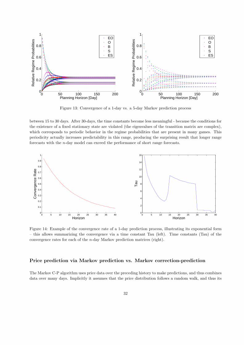
0 50 100 150 2000

0.2

0.4

0.6

0.8

1

Planning Horizon [Day]

Rel

ativ

e R

egim

e P

roba

bilit

ies

EOOBSES

0 50 100 150 2000

0.2

0.4

0.6

0.8

1

Planning Horizon [Day]

Rel

ativ

e R

egim

e P

roba

bilit

ies

EOOBSES

Figure 13: Convergence of a 1-day vs. a 5-day Markov prediction process

between 15 to 30 days. After 30-days, the time constants become less meaningful - because the conditions for

the existence of a fixed stationary state are violated (the eigenvalues of the transition matrix are complex),

which corresponds to periodic behavior in the regime probabilities that are present in many games. This

periodicity actually increases predictability in this range, producing the surprising result that longer range

forecasts with the n-day model can exceed the performance of short range forecasts.

0 5 10 15 20 25 30 35 400

0.1

0.2

0.3

0.4

0.5

0.6

0.7

0.8

0.9

1

Horizon

Con

verg

ence

Rat

e

0 5 10 15 20 25 30 35 400

2

4

6

8

10

12

14

16

Horizon

Tau

Figure 14: Example of the convergence rate of a 1-day prediction process, illustrating its exponential form

– this allows summarizing the convergence via a time constant Tau (left). Time constants (Tau) of the

convergence rates for each of the n-day Markov prediction matrices (right).

Price prediction via Markov prediction vs. Markov correction-prediction

The Markov C-P algorithm uses price data over the preceding history to make predictions, and thus combines

data over many days. Implicitly it assumes that the price distribution follows a random walk, and thus its

32

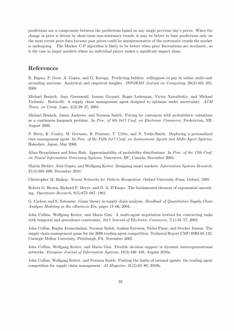
predictions are a compromise between the predictions based on any single previous day’s prices. When the

change in price is driven by short-term non-stationary trends, it may be better to base predictions only on

the most recent price data because past prices could be unrepresentative of the systematic trends the market

is undergoing. The Markov C-P algorithm is likely to be better when price fluctuations are stochastic, as

is the case in larger markets where no individual player makes a significant impact alone.

References

R. Bapna, P. Goes, A. Gupta, and G. Karuga. Predicting bidders: willingness to pay in online multi-unit

ascending auctions: Analytical and empirical insights. INFORMS Journal on Computing, 20(3):345–355,

2008.

Michael Benisch, Amy Greenwald, Ioanna Grypari, Roger Lederman, Victor Naroditskiy, and Michael

Tschantz. Botticelli: A supply chain management agent designed to optimize under uncertainty. ACM

Trans. on Comp. Logic, 4(3):29–37, 2004.

Michael Benisch, James Andrews, and Norman Sadeh. Pricing for customers with probabilistic valuations

as a continuous knapsack problem. In Proc. of 8th Int’l Conf. on Electronic Commerce, Fredericton, NB,

August 2006.

P. Berry, K. Conley, M. Gervasio, B. Peintner, T. Uribe, and N. Yorke-Smith. Deploying a personalized

time management agent. In Proc. of the Fifth Int’l Conf. on Autonomous Agents and Multi-Agent Systems,

Hakodate, Japan, May 2006.

Alina Beygelzimer and Irina Rish. Approximability of probability distributions. In Proc. of the 17th Conf.

on Neural Information Processing Systems, Vancouver, BC, Canada, December 2003.

Martin Bichler, Alok Gupta, and Wolfgang Ketter. Designing smart markets. Information Systems Research,

21(4):688–699, December 2010.

Christopher M. Bishop. Neural Networks for Pattern Recognition. Oxford University Press, Oxford, 1995.

Robert G. Brown, Richard F. Meyer, and D. A. D’Esopo. The fundamental theorem of exponential smooth-

ing. Operations Research, 9(5):673–687, 1961.

G. Cachon and S. Netessine. Game theory in supply chain analysis. Handbook of Quantitative Supply Chain

Analysis Modeling in the eBusiness Era, pages 13–66, 2004.

John Collins, Wolfgang Ketter, and Maria Gini. A multi-agent negotiation testbed for contracting tasks

with temporal and precedence constraints. Int’l Journal of Electronic Commerce, 7(1):35–57, 2002.

John Collins, Raghu Arunachalam, Norman Sadeh, Joakim Ericsson, Niclas Finne, and Sverker Janson. The

supply chain management game for the 2006 trading agent competition. Technical Report CMU-ISRI-05-132,

Carnegie Mellon University, Pittsburgh, PA, November 2005.

John Collins, Wolfgang Ketter, and Maria Gini. Flexible decision support in dynamic interorganizational

networks. European Journal of Information Systems, 19(3):436–448, August 2010a.

John Collins, Wolfgang Ketter, and Norman Sadeh. Pushing the limits of rational agents: the trading agent

competition for supply chain management. AI Magazine, 31(2):63–80, 2010b.

33

A. P. Dempster, N. M. Laird, and D. B. Rubin. Maximum likelihood from incomplete data via the EM

algorithm. J. of the Royal Stat. Soc., Series B, 39(1):1–38, 1977.

Richard O. Duda, Peter E. Hart, and David G. Stork. Pattern Classification (2nd Edition). Wiley-

Interscience, 2000.

W. Elmaghraby and P. Keskinocak. Dynamic pricing in the presence of inventory considerations: Research

overview, current practices, and future directions. Management Science, 49(10):1287–1309, 2003.

M. Fan, J. Stallaert, and A. B. Whinston. Decentralized mechanism design for supply chain organizations

using an auction market. Information Systems Research, 14(1):1–22, 2003.

S. Fine, Y. Singer, and N. Tishby. The hierarchical hidden markov model: Analysis and applications.

Machine learning, 32(1):41–62, 1998.

Rayid Ghani. Price prediction and insurance for online auctions. In Int’l Conf. on Knowledge Discovery in

Data Mining, pages 411–418, Chicago, Illinois, August 2005.

Anindya Ghose, Michael D. Smith, and Rahul Telang. Internet exchanges for used books: An empirical

analysis of product cannibalization and welfare impact. Information Systems Research, 17(1):3–19, 2006.

Jean Dickinson Gibbons. Nonparametric statistical inference. Technometrics, 28(3):275, 1986.

J.A. Gray and D.E. Spencer. Price prediction errors and real activity: A reassessment. Economic Inquiry,

28(4):658–681, 1990.

Alok Gupta, Dale O. Stahl, and Andrew Whinston. The Internet: A Future Tragedy of the Commons? In

H. Amman, B. Rustem, and A. B. Whinston, editors, Computational Approaches to Economic Problems,

pages 347–361, Dordrecht, The Netherlands, 1997. Kluwer Academic Publishers.

Minghua He, Alex Rogers, Xudong Luo, and Nicholas R. Jennings. Designing a successful trading agent for

supply chain management. In Proc. of the Fifth Int’l Conf. on Autonomous Agents and Multi-Agent Systems,

pages 1159–1166, May 2006.

Myles Hollander and Douglas A. Wolfe. Nonparametric statistical methods. Journal of the American

Statistical Association, 95(449):333, 2000.

Patrick R. Jordan, Christopher Kiekintveld, and Michael P. Wellman. Empirical game-theoretic analysis

of the TAC supply chain game. In Proc. of the Sixth Int’l Conf. on Autonomous Agents and Multi-Agent

Systems, pages 1188–1195, May 2007.

Ajit Kambil and Eric van Heck. Reengineering the Dutch flower auctions: A framework for analyzing

exchange organizations. Information Systems Research, 9(1):1–19, 1998.

S. Kaplan and M. Sawhney. E-hubs: the new B2B (business-to-business) marketplaces. Harvard business

review, 78(3):97–103, 2000.

N. Karmarkar. A new polynomial-time algorithm for linear programming. In Proceedings of the sixteenth

annual ACM symposium on Theory of computing, page 311. ACM, 1984. ISBN 0897911334.

Wolfgang Ketter. Identification and Prediction of Economic Regimes to Guide Decision Making in Multi-

Agent Marketplaces. PhD thesis, University of Minnesota, Twin-Cities, USA, January 2007.

34

Wolfgang Ketter, Elena Kryzhnyaya, Steven Damer, Colin McMillen, Amrudin Agovic, John Collins, and

Maria Gini. MinneTAC sales strategies for supply chain TAC. In Int’l Conf. on Autonomous Agents and

Multi-Agent Systems, pages 1372–1373, New York, July 2004.

Wolfgang Ketter, John Collins, Maria Gini, Alok Gupta, and Paul Schrater. A Computational Approach

to Predicting Economic Regimes in Automated Exchanges. In Proc. of the Fifteenth Annual Workshop on

Information Technologies and Systems, pages 147–152, Las Vegas, Nevada, USA, December 2005.

Wolfgang Ketter, John Collins, Maria Gini, Alok Gupta, and Paul Schrater. Detecting and Forecasting

Economic Regimes in Multi-Agent Automated Exchanges. Decision Support Systems, 47(4):307–318, 2009.

Wael Khreich, Eric Granger, Ali Miri, and Robert Sabourin. On the memory complexity of the forward-

backward algorithm. Pattern Recognition Letters, 31(2):91–99, 2010. ISSN 0167-8655.

Christopher Kiekintveld, Jason Miller, Patrick R. Jordan, Lee F. Callender, and Michael P. Wellman. Fore-

casting market prices in a supply chain game. Electronic Commerce Research and Applications, 8(2):63 –

77, 2009. ISSN 1567-4223. Special Section: Supply Chain Trading Agent Research.

P. R. Kleindorfer and D. J. Wu. Integrating long-and short-term contracting via business-to-business ex-

changes for capital-intensive industries. Management Science, pages 1597–1615, 2003.

I. Kontogounis, K.C. Chatzidimitriou, A.L. Symeonidis, and P.A. Mitkas. A robust agent design for dynamic

SCM environments. Proceedings of the 4th Hellenic Joint Conference on Artificial Intelligence (SETN),

Heraklion, Greece, pages 127–136, 2006.

Solomon Kullback. Information Theory and Statistics. Dover Publications, New York, 1959.

Solomon Kullback and Richard A. Leibler. On information and sufficiency. Annals of Mathematical Statistics,

22:79–86, 1951.

Richard Lawrence. A machine learning approach to optimal bid pricing. In 8th INFORMS Computing

Society Conf. on Optimization and Computation in the Network Era, pages 1–22, Arizona, January 2003.

Bill Mark and Raymond C. Perrault. Calo: Cognitive assistant that learns and organizes.

http://www.ai.sri.com/project/CALO, 2006.

Cade Massey and George Wu. Detecting regime shifts: The causes of under- and overestimation. Management

Science, 51(6):932–947, 2005.

Tom M. Mitchell. Mchine Learning. McGraw-Hill, 1997. ISBN: 0071154671.

J.F. Muth. Rational expectations and the theory of price movements. Econometrica, 29(3):315–335, 1961.

Ian T. Nabney. NETLAB Algorithms for Pattern Recognition. Springer, 2001.

Venu Nagali, Jerry Hwang, David Sangheraand Matt Gaskins, Mark Pridgen, Tim Thurston, Patty Mack-

enroth, Dwight Branvold, Patrick Scholler, and Greg Shoemaker. Procurement risk management (PRM) at

Hewlett-Packard company. Interfaces, 38(1):51–60, 2008.

FJ Nogales, J. Contreras, AJ Conejo, and R. Espinola. Forecasting next-day electricity prices by time series

models. IEEE Transactions on Power Systems, 17(2):342–348, 2002. ISSN 0885-8950. doi: 10.1109/TP-

WRS.2002.1007902.

35

Denise R. Osborn and Marianne Sensier. The prediction of business cycle phases: financial variables and

international linkages. National Institute Econ. Rev., 182(1):96–105, 2002.

David Pardoe and Peter Stone. Bidding for customer orders in TAC SCM: A learning approach. In Workshop

on Trading Agent Design and Analysis at AAMAS, pages 52–58, New York, July 2004.

David Pardoe and Peter Stone. Tactex-05: A champion supply chain management agent. In Proc. of the

Twenty-First National Conference on Artificial Intelligence, pages 1389–1394, Boston, Mass., July 2006.

AAAI.

Koen Pauwels and Dominique Hanssens. Windows of change in mature markets. In European Marketing

Academy Conf., Braga, Portugal, May 2002.

Vedran Podobnik, Anna Petric, and Gordan Jezic. An agent-based solution for dynamic supply chain

management. Journal of Universal Computer Science, 14(7):1080–1104, 2008. ISSN 0948-695X.

Stuart Russell and Peter Norvig. Artificial Intelligence - A Modern Approach; 2nd Edition. Prentice Hall,

2002. ISBN: 0137903952.

Tuomas Sandholm. Expressive commerce and its application to sourcing: How we conducted $35 billion of

generalized combinatorial auctions. AI Magazine, 28(3):45–58, 2007.

Claude E. Shannon. A mathematical theory of communication. Bell System Technical Journal, 27(3):379–423

and 623–656, July and October 1948.

Galit Shmueli. To explain or to predict? Statistical Science, 25(3):289–310, 2010.

Eric Sodomka, John Collins, and Maria Gini. Efficient statistical methods for evaluating trading agent

performance. In Proc. of the Twenty-Second National Conference on Artificial Intelligence, pages 770–775,

2007.

J. M. Swaminathan and S. R. Tayur. Models for supply chains in e-business. Management Science, 49(10):

1387–1406, 2003.

J.M. Swaminathan, S.F. Smith, and N.M. Sadeh. Modeling supply chain dynamics: A multiagent approach.

Decision Sciences, 29(3):607–632, 1998.

D. Titterington, A. Smith, and U. Makov. Statistical Analysis of Finite Mixture Distributions. Wiley, New

York, 1985.

Shanshan Wang, Wolfgang Jank, and Galit Shmueli. Explaining and forecasting online auction prices and

their dynamics using functional data analysis. Journal of Business and Economic Statistics, 26(2):144–160,

2008. ISSN 0735-0015.

Dongmo Zhang, Kanghua Zhao, Chia-Ming Liang, Gonelur Begum Huq, and Tze-Haw Huang. Strategic

trading agents via market modeling. SIGecom Exchanges, 4(3):46–55, 2004.

Xiaofeng Zhang and William K. Cheung. Learning global models based on distributed data abstractions. In

Nineteenth International Joint Conference on Artificial Intelligence, pages 1645–1646, Edinburgh, Scottland,

August 2005.

Wen Zhao and Yu-Sheng Zheng. Optimal dynamic pricing for perishable assets with nonhomogeneous

demand. Management Science, 46(3):375–388, 2000.

36