real-time visualization of unsteady vector …gerlebacher/home/publications/reno_2002... ·...

1 American Institute for Aerospace and Aeronautics

REAL-TIME VISUALIZATION OF UNSTEADY VECTOR FIELDS

M. Y. Hussaini*, Gordon Erlebacher†, Bruno Jobard‡ Florida State University, Tallahassee, FL 32306

Abstract We propose a new technique to visualize dense vector fields associated with unsteady fluid flows. This tech-nique is based on a Lagrangian-Eulerian Advection (LEA) scheme, and it enables animations with high spa-tio-temporal correlation at interactive rates. We demon-strate the efficiency and efficacy of the technique in applications to numerical simulation of a shock interact-ing with a longitudinal vortex, and of ocean circulation in the Gulf of Mexico. The simplicity of the data struc-tures and the facility of implementation suggest that LEA could become a useful component of any scientific visualization toolkit concerned with the display of un-steady flows.

Introduction Several techniques have been developed for the dense representation of unsteady vector fields. The best known technique is perhaps due to Shen1 who devel-oped UFLIC (Unsteady Flow LIC). Based on the Line Integral Convolution (LIC) scheme2, it achieves good spatial and temporal correlation. However, the images are difficult to interpret as the pathlines or streamlines become blurred in regions of rapid change of direction, and thicken where the flow is almost uniform. This drawback is due to the large number of particles (three to five times the number of pixels in the image) that need to be processed for each animation frame.

The spot noise technique, originally developed for the visualization of steady vector fields, has been naturally extended to include unsteady flows3. It employs a suffi-ciently large collection of elliptic spots to cover entirely an image of the physical domain. The position of these spots is integrated along the flow, their shape is bent along the local pathline or streamline, and the resulting

* Professor, TMC Eminent Scholar. † Professor, Department of Mathematics, Senior Meme-

ber. ‡ Researcher, Swiss Center for Scientific Computing,

Switzerland. Copyright © 2001 American Institute of Aeronautics

and Astronautics, Inc. All rights reserved.

image is finally blended into the animation frame. In this technique, the rendering speed is increased by de-creasing the number of spots in the image and the pixel coverage is controlled by assigning a fixed lifespan to each spot.

Max and Becker4 proposed a texture-based technique that advects a texture along the flow either by advecting the vertices of a triangular mesh or by integrating the texture coordinates associated with each triangle back-ward in time. When texture coordinates or particles leave the physical domain, an external velocity field is linearly extrapolated from the boundary. This technique attains interactive frame rates by controlling the resolu-tion of the underlying mesh.

A technique to display streaklines was developed by Rumpf and Becker5. They precompute a two-dimensional noise texture whose coordinates represent time and a boundary Lagrangian coordinate. Particles at any point in space and time that originate from an in-flow boundary are mapped back to a point in this tex-ture.

More recently, Jobard et al.6,7 extended the work of Heidrich et al.8 to animate unsteady two-dimensional vector fields. The technique relies heavily on extensions to OpenGL proposed by SGI, in particular, pixel tex-tures, additive and subtractive blending, and color trans-formation matrices. They pay particular attention to the flow entering and leaving the physical domain, leading to smooth animations of arbitrary duration. Excessive discretization errors associated with 12 bit textures are addressed by a tiling mechanism9. Unfortunately, the graphics hardware extension, specifically the pixel tex-ture extension, on which this algorithm relies most, is not adopted by other graphics card manufacturers. As a result, the algorithm runs at present only on the SGI Maximum Impact and the SGI Octane with the MXE graphics card.

In this paper, we propose a new visualization technique that combines the advantages of what are called La-grangian and Eulerian formalisms. A dense collection of particles is integrated backward in time (Lagrangian step), while the color distribution of the image pixels is updated in place (Eulerian step). The dynamic data structures normally required to track individual parti-cles, pathlines, or streaklines are no longer necessary since all information is now stored in a few two-

2002-0749


dimensional arrays. The combination of Lagrangian and Eulerian updates is repeated at every iteration. A single time step is executed as a sequence of identical opera-tions over all array elements. By its very nature, the algorithm takes advantage of spatial locality and in-struction pipelining and can generate animations at in-teractive frame rates.

Problem Statement We track the evolution of a dense collection of parti-cles, tagged by their position X at some fixed time, immersed in a time-dependent velocity field. The posi-tion x of each particle depends on X and time t :

( , ) ( )tt= =x x X x X , (1)

and the velocity of this particle is simply the time derivative of its position:

( , )

( , ) ( )td tt

dt= =x X

v X v X . (2)

At any time t , there is a one-to-one mapping between the position x of a particle and its label X . Therefore, (1) is invertible:

( , ) ( )tt= =X X x X x .

As the particle advects with the flow velocity, its label remains constant so that its variation along a particle path vanishes:

( )( )( ) 0

tt t

t

∂ + ⋅ ∇ =∂

X xv X X x . (3)

When x is viewed as an independent variable, the par-ticular particle tX that passes through x changes in time. In a similar manner, any material (or particle) property ( ( ))tF X x constant along a particle path satis-fies 0dF = , or

( )( ) ( ) ( )( ) 0

t

t tF

Ft

∂+ ⋅ ∇ =

∂X x

v x X x (4)

An Eulerian approach solves (4) directly for the mate-rial property as a function of x; as a result, particles lose their identity. In exchange, the particle property, viewed as a field, is known for all time at any spatial location.

A Lagrangian approach solves (2) where ( )tx X is physically interpreted to mean the trajectory of a parti-cle X . In this approach, the trajectory of each particle is computed separately, and the time evolution of a col-lection of particles is displayed by rendering each parti-cle by a glyph (point, texture spot, arrow). With the exception of the recent work of Jobard et al.6,7 and Rumpf and Becker5, current time-dependent algorithms are all based on particle tracking, e.g.,1,3,4,10. While La-grangian tracking is well suited to the task of under-standing how dense groups of particles evolve in time, it suffers from several shortcomings. For example, in re-

gions of flow convergence, particles may accumulate into small clusters that follow almost identical trajecto-ries, leaving regions of flow divergence with a low den-sity of particles. To maintain a dense coverage of the domain, the data structures must support dynamic inser-tion and deletion of particles1, or track more particles than needed3, which often decreases the efficiency of any numerical implementation. On the other hand, an explicit discretization of (4) is subject to a Courant-Friedrich-Levy (CFL) condition, which limits the speed of the flow animation as seen by the user.

Methodology We propose a new algorithm, called the Lagrange-Euler-Advection (LEA) approach, which builds on the strengths of both the Eulerian and Lagrangian ap-proaches to particle advection. In this approach, the coordinates of a dense collection of particles (placed at every pixel of a destination image) are tracked between two successive time steps with a Lagrangian scheme, whereas the property field is subject to an Eulerian up-date. At the beginning of each iteration, a new dense collection of particles is chosen and assigned the prop-erty computed at the end of the previous iteration.

To illustrate the idea, consider the advection of the bit-map image shown in Figure 1a by a circular vector field centered at the lower left corner of the image. With a pure Lagrangian scheme, a dense collection of particles (one per pixel) is first assigned the color of the corre-sponding underlying pixel. Each particle advects along the vector field and deposits its color property in the corresponding pixel in a new bitmap image. This tech-nique does not ensure that every pixel of the new image is updated. Indeed, holes usually appear in the resulting image (Figure 1b). To avoid such holes, our scheme considers each pixel of the new image as a particle, and it is updated with the color of the bitmap that the parti-cle initially occupied, obtained by integrating backward in time (Figure 1c). Repeating the process at each itera-tion, any property can be advected while maintaining a dense coverage of the domain.

Thus, the core of the advection process is the composi-tion of two basic operations: coordinate integration and property advection.

Given the position ( ) ( )0 , ,i j i j=x of a particle in an image at pixel ( ),i j , backward integration of Equation (2) over a time interval h determines its position

Figure 1. Rotation of bitmap image about the lower left corner. (a) Original image, (b) Image rotated with Lagrangian scheme, (c) Image rotated with Eulerian scheme.


( ) ( ) ( )( )0

0

, , ,h

h ti j i j i j dτ τ τ−

− += + ∫x x v x (5)

at a previous time step. h is the integration step, ( ),i jτx represents intermediary positions along the

pathline passing through ( ),t i jx , and τv is the vector field at time τ .

From (5) it follows that an image of resolution W H× , defined at a previous time t h− , is advected to time t through the indirection operation

( ) ( )( ) [ ) [ ), 0, 0,,

user-specified value otherwise

t h h ht i j W H

i j− − − ∀ ∈ ×=

I x xI

(6)

which allows the image at time t to be computed from the image at any prior time t h− . This technique was used by Max4 with h t= . However, instead of integrat-ing back to the initial time to advect the initial texture, we choose h to be the interval between two successive images and always advect the last computed frame. This minimizes the need to access coordinate values outside the physical domain and eliminates texture distortion4. To compute an image of acceptable quality from t h−I evaluated at h−x , at least linear interpolation is neces-sary.

Algorithm In the Lagrangian-Eulerian approach, a full per-pixel advection requires manipulating exactly W H× parti-cles. Information attached to a given particle at pixel ( ),i j is stored in two-dimensional arrays of resolution W H× at the corresponding index location ( ),i j . Thus, we store the initial coordinates ( ),x y of the par-ticles in two arrays ( ),x i jC and ( ),y i jC . Two arrays

x′C and y′C contain their x - and y - coordinates after integration along pathlines. A first order integration method requires two arrays xV and yV that store the velocity field at the current time. Similar to LIC, we choose to advect noise images. Four noise arrays N ,

′N , aN and bN contain, respectively, the noise to advect, two advected noise images, and the final blended image.

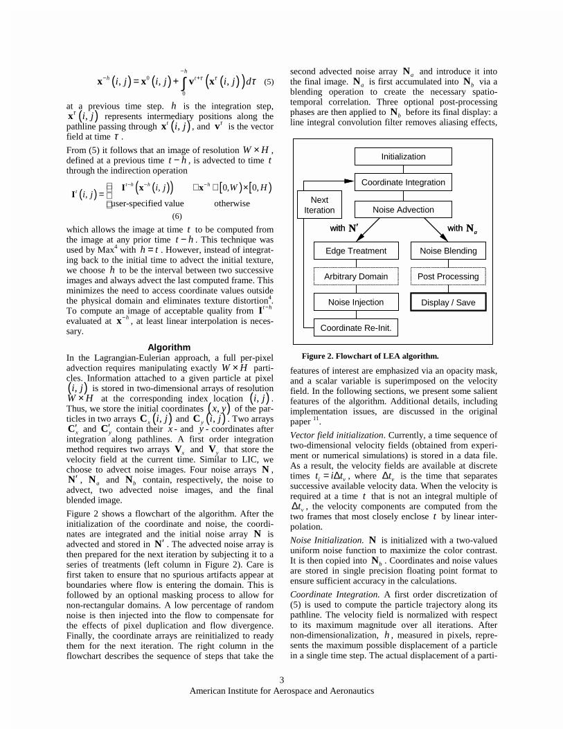
Figure 2 shows a flowchart of the algorithm. After the initialization of the coordinate and noise, the coordi-nates are integrated and the initial noise array N is advected and stored in ′N . The advected noise array is then prepared for the next iteration by subjecting it to a series of treatments (left column in Figure 2). Care is first taken to ensure that no spurious artifacts appear at boundaries where flow is entering the domain. This is followed by an optional masking process to allow for non-rectangular domains. A low percentage of random noise is then injected into the flow to compensate for the effects of pixel duplication and flow divergence. Finally, the coordinate arrays are reinitialized to ready them for the next iteration. The right column in the flowchart describes the sequence of steps that take the

second advected noise array aN and introduce it into the final image. aN is first accumulated into bN via a blending operation to create the necessary spatio-temporal correlation. Three optional post-processing phases are then applied to bN before its final display: a line integral convolution filter removes aliasing effects,

features of interest are emphasized via an opacity mask, and a scalar variable is superimposed on the velocity field. In the following sections, we present some salient features of the algorithm. Additional details, including implementation issues, are discussed in the original paper 11.

Vector field initialization. Currently, a time sequence of two-dimensional velocity fields (obtained from experi-ment or numerical simulations) is stored in a data file. As a result, the velocity fields are available at discrete times i vt i t= ∆ , where vt∆ is the time that separates successive available velocity data. When the velocity is required at a time t that is not an integral multiple of

vt∆ , the velocity components are computed from the two frames that most closely enclose t by linear inter-polation.

Noise Initialization. N is initialized with a two-valued uniform noise function to maximize the color contrast. It is then copied into bN . Coordinates and noise values are stored in single precision floating point format to ensure sufficient accuracy in the calculations.

Coordinate Integration. A first order discretization of (5) is used to compute the particle trajectory along its pathline. The velocity field is normalized with respect to its maximum magnitude over all iterations. After non-dimensionalization, h , measured in pixels, repre-sents the maximum possible displacement of a particle in a single time step. The actual displacement of a parti-

Initialization

Coordinate Integration

Edge Treatment

Arbitrary Domain

Noise Injection

Coordinate Re-Init.

Noise Blending

Post Processing

Display / Save

Noise Advection

′N aNwith with

Next Iteration

Initialization

Coordinate Integration

Edge Treatment

Arbitrary Domain

Noise Injection

Coordinate Re-Init.

Noise Blending

Post Processing

Display / Save

Noise Advection

′N aNwith with

Next Iteration

Figure 2. Flowchart of LEA algorithm.


cle is proportional to the local velocity and is measured in units of cell widths.

Noise Advection. The advection of noise described by (6) is applied twice to N to produce two noise arrays:

′N for advection and aN for display. ′N is an inter-nal noise array whose sole purpose is to track the advec-tion process and serve as the initial noise array for the next iteration. To maintain a sufficiently high contrast in the advected noise, ′N is computed with a constant interpolation. A linear interpolation would produce “gray” noise and become uniformly gray after several iterations. Before ′N can be used in the next iteration, it must undergo a series of corrections to account for edge effects, the presence of arbitrary domains, and the deleterious consequences of flow divergence. The high contrast of ′N is not suitable for display. To remedy the situation, we simultaneously compute a noise array

aN from N using linear interpolation, which decreases spatial aliasing. Although some contrast is lost, this is only done once with a high contrast source. aN partici-pates in the creation of the current animation frame through alpha blending with bN .

A straightforward implementation of (6) leads to condi-tional expressions to handle the cases when

( ) ( )( ), , ,x yi j i j′ ′ ′=x C C is exterior to the physical domain. A more efficient implementation eliminates the need to test for boundary conditions by surrounding N and ′N with a buffer zone of constant width b h= cell widths.

Edge Treatment. A recurring issue with texture advec-tion is the proper treatment of information flowing into the physical domain. Within the context of this paper, we must determine the user-specified value in Equation (6). We recall that the advected image contains a two-valued random noise with little or no spatial correlation. We take advantage of this property to replace the user-specified value by a random value. At each iteration, new random noise is stored in the buffer zone, at negli-gible cost. Particles that were outside the physical do-main at the previous time step carry a random property value into the domain. Since random noise has no spa-tial correlation, the advection of the surrounding buffer values into the interior region of ′N produces no visi-ble artifacts.

Incoming Flow in Arbitrary- Shape Domains. It often happens that the physical domain is non-rectangular or contains interior regions where the flow is not defined (e.g. shores and islands). Denote by B the boundaries interior to N that delineate these regions. LEA handles this case with no modification by simply setting the velocity to zero where it is not defined. The stationary noise in these regions is hidden from the animation frame by superimposing a semitransparent map that is opaque where the flow is undefined.

Noise Injection. When particles in neighboring cells of ′N retrieve their property value from within the same

cell of N , the property value (i.e., the particle color)

will be duplicated in the corresponding cells of N . This duplication process will propagate over time, increasing

the spatial correlation of the noise between adjacent image pixels. To illustrate the effect of this duplication, we show in Figure 3 two time frames of the interaction of a shock with a longitudinal vortex (see Result Sec-tion). In the right column the effect of pixel duplication is clearly seen: at later time (bottom figure), areas of constant color have expanded. This effect is undesirable since lower noise frequency reduces the spatial resolu-tion of the features that can be represented. This dupli-cation effect is further reinforced in regions where the flow has a strong positive divergence. Note that these images correspond to several successive frames blended together. The corresponding unblended images at the later time, shown in Figure 3 clearly show that the noise array has increased its spatial correlation.

To break the formation of uniform blocks and to main-tain a high frequency random noise, we inject a user-specified percentage of noise into ′N . Random cells are chosen in ′N and their value is inverted (a zero value becomes one and vice versa). The number of cells ran-domly inverted must be sufficiently high to eliminate the appearance of pixel duplication, but low enough to maintain the temporal correlation introduced by the advection step. The effect of this procedure is seen in the left column of Figure 3.

Coordinate Re-Initialization The final step is to re-initialize the coordinate arrays to prepare a new collection of particles for the next itera-tion. Unfortunately, our use of constant interpolation to compute the particle property at the previous time step (to avoid a rapid loss of contrast), would “freeze” the flow in regions where the velocity magnitude is too low. A property value can only change if it originates from a different cell. If the coordinate arrays were re-initialized

Figure 3. Two frames of animation: frame 25 (top) and 95 (middle, bottom). Two percent noise injec-tion (middle), no noise injection (bottom). Blended image (left), noise texture (right).


to their original values at each iteration, sub-cell dis-placements would be ignored and the flow would be frozen where the velocity magnitude is too low. This is illustrated in Figure 4, which shows the advection of a steady circular vector field. Constant interpolation without fractional coordinate tracking clearly shows that the flow is partitioned into distinct regions within which the integer displacement vector is constant (Figure 4a). To prevent this, we track the fractional part of the dis-placement within each cell. Instead of re-initializing the coordinates to their initial values, the fractional part of the displacement is added to cell indices. The effect of this correction is shown in Figure 4b.The coordinate arrays have now returned to the state in which they were after their initialization phase.

Noise Blending. Although successive advected noise arrays are correlated in time, each individual frame re-mains devoid of spatial correlation. By applying a tem-poral filter to successive frames, spatial correlation is introduced. We store the result of the filtering process in an array bN . We find the exponential filter to be convenient, since its discrete version only requires the current advected noise and the previous filtered frame. It is implemented as an alpha blending operation

(1 )b b aα α= − +N N N , (7)

where α represents the opacity of the current advected noise array. A typical range for α is [ ]0.05,0.2 . Fig-ure 5 shows the effect of α on images based on the same set of noise arrays.

The blending stage is crucial because it introduces spa-tial correlation along pathline segments in every frame. To show clearly that the spatial correlation occurs along pathlines passing through each cell, we conceptualize the algorithm in 3D space; the x - and y - axes repre-sent the spatial coordinates, whereas the third axis is time. To understand the effect of the blending opera-tion, let’s consider an array N with black cells and change a single cell to white. During advection, a se-quence of noise arrays (stacked along the time axis) is generated in which the white cell is displaced along the flow. By construction, the curve followed by the white cell is a pathline. The temporal filter blends successive

noise arrays aN with the most recent data weighted more strongly. The temporal blend of these noise arrays produces the projection of the pathline onto the x y− plane, with an exponentially decreasing intensity as one travels back in time along the pathline. When the noise array with a single white cell is replaced by a two-color noise distribution, the blending operation introduces spatial correlation along a dense set of short pathlines.

Streamlines and pathlines passing through the same cell at the same time are tangent to each other, so a stream-line of short extent is well approximated by a short pathline. Therefore, a collection of short pathlines

serves to approximate the instantaneous direction of the flow. With our LEA technique, a single frame repre-sents the instantaneous structure of the flow (stream-lines), whereas an animated sequence of frames reveals the motion of a dense collection of particles released into the flow.

We illustrate the temporal correlation in Figure 5, which is a small area in the animation of flow over a circular cylinder (wake region). The three frames shown are separated by five iterations. Two regions are marked (white square and circle) to draw attention to the advec-tion of a particular flow structure.

(a) (b)(a) (b)

Figure 4. Circular flow without (left) and with (right) accumulation of fractional displacement (h=2).

α=0.10

α=1.00

α=0.50

α=0.03

α=0.10

α=1.00

α=0.50

α=0.03

Figure 5. Frames obtained with different values of . .

Figure 6. Small area from the wake region of an animation of flow past a circular cylinder. Three successive frames from the flow field are shown to demonstrate the temporal correlation. The white shapes identify a fixed location in space to help visualize the feature advecting with the flow.


Post-Processing A series of optional post-processing steps is applied to

bN to enhance the image quality and to remove fea-tures of the flow that are uninteresting to the user. A fast version of LIC can be applied to remove high frequency content in the image, a velocity mask serves to draw attention to regions of the flow with strong currents, and a scalar variable overlay allows the simultaneous visu-alization of an animated flow field and time evolution of a user-specified scalar field.

Directional Low-Pass Filtering (LIC). By construction, the noise in the advected images is of high frequency and high contrast. After blending, bN retains some residual effects of these high frequencies due to aliasing artifacts. Experimentation with different low-pass filters led us to conclude that a Line Integral Convolution filter applied to bN is the best filter to remove the effects of high frequency while preserving and enhancing the di-rectional correlation resulting from the blending phase. Although image quality is often enhanced with longer kernel lengths, it is detrimental here since the resulting streamlines will have significant deviations from the actual pathlines. The partial destruction of the temporal correlation between frames would lead to flashing ef-fects in the animation. A secondary effect of longer ker-nels is decreased contrast.

In general, a filter length L h≈ produces a smooth image with no aliasing. However, large values of h speed up the flow, with a resulting increase in aliasing effects (Figure 7). If the quality of the animation is im-portant, L must be increased with a resulting slowdown in the frame rate. As shown in Table 1, smoothing the velocity field with LIC reduces the frame rate by a fac-tor of three on the various computer architectures and operating systems the algorithm was benchmarked on. We recommend exploring the data at higher resolution without the filter or at low resolution with the filter.

We have implemented a software version of the algo-rithm developed in Heidrich8; the source code can be found in 11.

Velocity Mask and Background Image. A straightfor-ward implementation of the texture advection algorithm described so far produces static images that show the flow streamlines and interactive animations that show the motion for the flow along pathlines. The length of the streaks is statistically proportional to the flow veloc-ity magnitude. Additional information can be encoded into the images by modulating the color intensity ac-cording to one or more secondary variables.

It is often advantageous to superimpose the representa-tion of flow advection over a background image that provides additional context. An example is shown in Figure 8, which shows the ocean currents along with a background map colored with depth. In order to imple-ment this capability, the image must become partially transparent.

Two approaches have been implemented. First, we cou-ple the opacity of a pixel to its color intensity. Second, we modulate the pixel transparency with the magnitude of the velocity.

The blended image pixel color ranges from black to white. Neither color has a predominant role in repre-senting the velocity streaks. Therefore, one of these colors can be eliminated and therefore made partially transparent. We consider a black pixel to be transparent, and a while pixel to be fully opaque. The transfer func-tion that links these two states is a power law.

Regions of the flow that are nearly stationary add little useful information to the view. For example, regions of high velocity are often of most interest in wind and ocean current data. Accordingly, we also modulate the transparency of each pixel according to the velocity magnitude. This produces a strong correlation between the length of the velocity streaks and their opacity.

The ideas described in the two previous paragraphs are implemented through an opacity map, also referred to as a velocity mask. Once computed, the velocity mask is combined with bN into an intensity-alpha texture that is blended with the background image. We define the opacity map

( )( ) ( )( )1 1 1 1m n

b= − − − −A V N (8)

as a product of a function of local velocity magnitude and a function of the noise intensity. Higher values of the exponents m and n increase the contrast between regions of low and high velocity magnitude, and low and high intensity, respectively. When 1m n= = , the opacity map reduces to

bA = VN

As the exponents are increased, the regions of high velocity magnitude and of high noise intensity increase their impor-tance relative to other regions in the flow.

Figure 7. Frame without (bottom) and with (top) LIC filter. A velocity mask is applied to both im-ages. Data courtesy Z. Ding.


Higher quality pictures that emphasize the velocity magnitude can also be obtained by replacing the noise texture with a scalar map of the velocity magnitude (with color ranging from black to white as the magni-tude ranges from zero to one) combined with positive exponents. As a result, the texture advection is seen through the opacity map.

Scalar Overlay. To further add to the information dis-played, a scalar variable can be superimposed over the image. Care must be taken to ensure that a proper bal-ance is achieved between the visibility of the scalar variable and the velocity field of the underlying flow. We compute the image of the time-dependent scalar function at every iteration by computing its value at the vertices of a uniform grid and displaying each cell using hardware Gouraud shading. The resolution of the grid is chosen by the user to strike a proper balance between enhanced spatial structure and maximum interactivity. Higher grid resolutions lead to lower frames rates. We currently map the range of the scalar variable linearly between two colors. The scalar field is stored in a sepa-rate image that is alpha-blended with bN to produce a composite image. The final image I is a linear combi-nation of B (the background texture), bN (the flow field), and S (the scalar function).

The correct weighing of the various terms is chosen on a case-by-case basis not to obfuscate bN or S . Clearly, automatic strategies for this selection are highly desir-able. Finally, we note that the scalar image is fully opaque. Judicious use of its opacity channel could fur-ther enhance the contrast between bN , S and N .

Parameters for Realistic Visualization The numerical algorithm decouples the choice of the time interval between successive velocity fields t∆ , and the displacement h of a particle with unit velocity magnitude. Unless the relationship between h and t∆ is consistent with the physics of the problem, the rate of change in the structure of the velocity field (determined by t∆ ) will not be consistent with the speed at which information is convected along the particle paths (de-termined by h ).

A physically realistic animation of an unsteady vector field must respect the spatio-temporal relationships be-tween the dimensions of the physical problem and that of the animation frames. By physically realistic, we mean that if some fluid property is at point A with co-ordinates ( ),A Ax y ϕ at physical time 0t ϕ and reaches point B ( ),B Bx y ϕ at 1t ϕ , a fluid element virtually tagged passing through ( ),A Ax y at 0t in an animation frame should pass through the location ( ),B Bx y at the corresponding animation time 1t′ . We have affixed a subscript ϕ to denote physical variables.

It is easy to find a system of linear equations that keeps constant ratios between physical and computational dimensions. Such a system links together dimensions of the physical phenomenon with noise texture resolution, integration step size, number of images in the anima-tion, and fractional increment between available vector fields. Aside from the physical parameters normally associated with a vector field, we propose a way to compute the other parameters that lead to visually pleas-ing, realistic-looking advection animations. This entails

Figure 8. Three frames of ocean circulation in the Gulf of Mexico.


adopting the proper balance between animation frame rate, and rate of evolution of property values along the streamlines. Note that sometimes we wish to accelerate the evolution of physical time to concentrate on the structural evolution of the flow, rather than on the prop-erty advection itself. As a result, the convection of noise along particle paths may be to rapid to discern properly on the chosen timescale. Either the user can reduce the motion of the particles with respect to the change of structure, thus breaking the physical realism, or he can simply ignore the particles moving along the paths. If the particles move at too rapid a rate, the paths may become overly blurred and hard to discern. At this time, the control of the parameters is a manual operation.

Among the visualization parameters, the integration step size h has the highest impact on images. Visually, it determines the maximum distance in cells a property can travel in a single iteration. If h is too small, the flow appears to be motionless. On the other hand, if h is too large, a fluid property in regions of high velocity is displaced several cells in a single iteration, decreas-ing the effectiveness of the temporal correlation. In practice, taking h between 2.0 and 5.0 produces consis-tently high quality visual results.

The relationship between parameters in physical and computational space is given by

images maxVhN V t

W Wϕ ϕ

ϕ

= , (9)

where maxVϕ is the maximum velocity component in the whole dataset, tϕ is the duration of the physical phe-nomenon, Wϕ is the width of the physical domain and W is the width (measured in number of cells) of the animation frame. Note that both sides of the equation are dimensionless. Our choice of normalization implies that 1V = .

The temporal slices are equally spaced in time; there-fore, image i in the animation is computed with the

vfin vector field, vf vf images

in iN N= , where vfN is the number of temporal slices available in the dataset, and

imagesN is the number of animation frames. The frac-tional part of vf

in is used to perform an interpolation of the vector field between the two nearest enclosing available fields.

The precise ratio between physical and computational linear time is most important for animations of time-dependent flows since it affects the rate at which the structure of the fluid changes with respect to the rate at which particles move along the pathlines. Getting the ratio correct is far less important when single time slices are shown (e.g., the figures in this paper). In this case, an incorrect ratio will shorten or lengthen the extent of blending along the particle path. However, the blending will always remain proportional to the fluid velocity. Since the scale factor is uniform, the relative distribu-tion of velocities is not affected.

Results We evaluated the efficiency of the algorithm on several computer architectures at three resolutions ( 2300 through 21000 pixels). In Table 1, timings in frames/second, are presented. The architectures consid-ered were a Dell Precision Workstation 530 (1.7 GHz Intel Xeon, 250 kbyte cache, 400 MHz bus, and a Quadro-2 Pro Nvidia card), an SGI Octane with EMXI graphics hardware (200 MHz R10000 MIPS processor, 4Mbyte of secondary cache), and a four-processor SGI Onyx (300 MHz R12000 MIPS processor, 12 Mbytes of secondary cache). Both serial and parallel (using OpenMP) benchmarks were conducted on the Onyx. The proposed algorithm is fully implemented in soft-ware with the exception of the 2D texture placement. Although all of the graphics cards support hardware texture operations, the software component of the algo-rithm dominates the computational time. The organiza-tion of the algorithm as a series of array operations makes it particularly straightforward to parallelize on shared memory architectures. Furthermore, operations on the array elements only make accesses within h rows or columns. Small h (< 5), moderate texture sizes ( 21000 ), and moderate secondary cache sizes (> 1 Mbyte), lead to very few cache misses, and thus very high efficiency. We have considered the options used most often. The highest frame rates correspond to the texture advection algorithm without masking or post-processing (the cost of the blending operation is insig-nificant). As expected, the Onyx produces the highest frame rates across all combinations of options and tex-ture resolutions. A parallel implementation of the algo-rithm on four processors produces a speedup of about a factor of three. Our Onyx has a single graphics pipe; all graphic primitives can only reach the graphics hardware through a single processor. As a result, calls to the OpenGL library are serialized. The effect of this seriali-zation becomes worse as the number of processors is increased. The cost of the masking operation ranges from 30 to 50 percent on the Onyx and Octanes, but only 10 percent on the Dell. The reason for this discrep-ancy is not known, although the Dell bus speed and their very fast processors are surely a factor. The LIC filter is extremely expensive relative to the base algo-rithm. Application of the filter at every time step leads to a 2 to 3-fold decrease in the frame rate relative to the base algorithm combined with masking. One of the rea-sons for this cost is that the LIC computation is totally recomputed at each step. The cost of the LIC is ap-proximately proportional to the length of the filter ker-nel. We expect that further optimization is possible by considering temporal coherence; however, have not pursued this idea.

We now now demonstrate the versatility of the Lagran-gian-Euler Advection technique by considering exam-ples from experimental fluid dynamics, computational fluid dynamics, and oceanic sciences.


Reso-lution

Advection Advection + Velocity Mask

( )3m n= =

Advection + Velocity Mask + LIC filter

( )6L =

9.7 14.0 8.7 8.8 2.6 3.0 300

16.3 39.0 10.4 27.0 3.6 11.6

3.5 4.7 3.2 3.1 0.93 1.0 500

6.3 18.0 3.7 10.5 1.3 4.5

NA 1.2 NA 0.7 NA 0.2 1000

1.4 4.1 0.9 2.7 0.3 1.1

Table 1: Timings in frames/second as a function of op-tions and resolutions. Each configuration has been tested on four different configurations: Dell Precision 530 Workstation with Quadro2-Pro video card (upper left), Octane (upper right), Onyx2 (lower left) and Onyx2 with four processors (lower right).

Gulf of Mexico

Shock

Grid size 352 320× 257 151×

Number of frames

183 300

Dataset (Mbytes)

165 93

Table 2: Characteristics of datasets used in the paper.

Ocean circulation in the Gulf of Mexico Recent numerical simulations at the Center for Ocean-Atmospheric Prediction Studies (COAPS) at Florida State University aim to reveal the detailed structure of ocean currents. The simulations are based on the Navy Coastal Ocean Model (NCOM). The data was obtained from a simulation at a resolution of 352 320 40× × using a third order upwind scheme for the horizontal advection terms and a second order discretization in the vertical direction. Each time step in the simulation is 400 seconds. The velocity field is stored at intervals of 48 hours (432 iterations in the simulation). The 183 frames provided correspond to a one-year simulation. The spatial domain extends from latitudes 15.55 ND to 31.55 ND and from longitudes 98.15 WD to 80.55 WD . The spatial grid is 0.05 degrees.

Figure 8 shows three frames of this flow at a single depth. The images are enhanced by first rendering a fixed background image of the topography of the ocean floor and surrounding land. A velocity mask is applied to the flow to enhance regions of high velocity magni-tude. As a result, regions of lowest opacity lie in areas

of low velocity magnitude, which renders the back-ground image partially visible. The flow has a compli-cated topology, composed of a series of localized vortices. From the sequence of images shown, the to-pology is also seen to be time-dependent. For example, the two vortices in the upper frame have merged in the lower frame. The strong temporal correlation and the interactive frame rates permit parametric investigations and make it possible to improve our intuition about the flow evolution.

For a noise texture size of 2512 and using four proces-sors on an SGI Onyx, we observe rates of approxi-mately 20 frames per second with masking turned off and 10 frames per second with masking turned on.

Shock-Vortex interaction An example of a strongly unsteady flow is the interac-tion of a shock with a vortex oriented with its axis nor-mal to the shock. Numerical simulations of this interaction were conducted under conditions of axi-symmetry12. In the chosen configuration, two uniform flow regions are separated by a plane shock of infinite extent. An isentropic vortex is superimposed on the mean flow. The vortex is a solution to the steady-state Euler equations and is convected towards the shock at the uniform upstream velocity. The radial profile decays exponentially to avoid numerical artifacts at the free-stream boundary. The numerical method is based on a formally third order ENO algorithm in space that main-tains sharp, essentially non-oscillatory, shock transi-tions.

We conducted a numerical simulation on a grid of 400 151× with a uniform grid in the streamwise direc-tion, and a grid concentrated near the centerline to bet-ter capture the vortex shock interactions that result from the interaction of the vortex core structure with the shock. The data was then interpolated to a 256 151× uniform grid over the same physical domain [ 7,2] [0,4]− × . The velocity field and the density gra-dient are read from 96 files on a grid of 256 151× . The velocity field is defined over a span of 50 time units. A unit time interval is the time it takes a fluid element to travel the distance of one vortex core diameter upstream of the shock. The dataset is composed of 200 frames, with a separation of 0.4 time units between successive frames.

We limit our examples to a Mach 7 shock and a unit vortex circulation12. To maximize the information con-tent, we superimpose the density gradient field over the advected texture. (The density gradient captures both the shock structures and the slip lines of the flow.) To better emphasize the density gradient, we compute the auxiliary scalar variable ( )maxexp /ρ ρ− and map it to a range of yellows, brighter in regions of higher gradi-ent, or lower scalar value. A transparency map is asso-ciated with, and proportional to, the scalar field. This allows the velocity field to show through regions of low


density gradient. We have found that the composite image of the velocity field and scalar field is strongly dependent on the precise mapping and transparency functions, thus leading to excessive trial and error on the part of the user. Additional research into the auto-matic selection of functional and color mappings is re-quired to minimize user intervention. From an imple-mentation standpoint, the density is drawn at the full resolution of the underlying velocity field using Gouraud shading. This technique was chosen, as op-posed to direct texture mapping, to avoid preprocessing the time-dependent scalar data and storing it into tex-tures prior to an interactive session. Furthermore, the user has control of the grid resolution on which the sca-lar field is defined. Since the cost of displaying a scalar function is proportional the grid that underlies it, in-creased interactivity is achieved by defining the scalar on two or more grids: coarser grids for higher interac-tivity, finer grids for static pictures, when the flow is steady, or when visualizing detailed structures is more important than interactive exploration.

A time sequence of the shock vortex interaction process is shown in Figure 9. Increasing time is from top to bot-tom, left to right. We have maximized information con-tent by combining a mask cubic in the noise intensity and cubic in the velocity magnitude. In the absence of a background texture, transparent pixels are black. The mask clearly brings into evidence the discontinuity of the velocity across the shock. A triple point structure and its associated slip line become well defined by the last frame in the left column. The figure also indicates that the velocity magnitude is very high and is strongly rotational in the region between the primary shock and the slip line. Dark regions correspond to areas where the flow is almost at a standstill. We should note that the velocity field is normalized across all frames of the animation. Therefore, a very bright region in the image indicates that the flow is near its maximum. The density gradient vividly shows internal structure in the flow. While the upstream structure is smooth inside the vor-tex, a complex network of secondary shocks and slip lines is visible downstream of the primary shock. In the last two frames, an intriguing inverted triple point shock, whose presence was unsuspected, is clearly seen. A more detailed analysis is necessary to determine its origin.

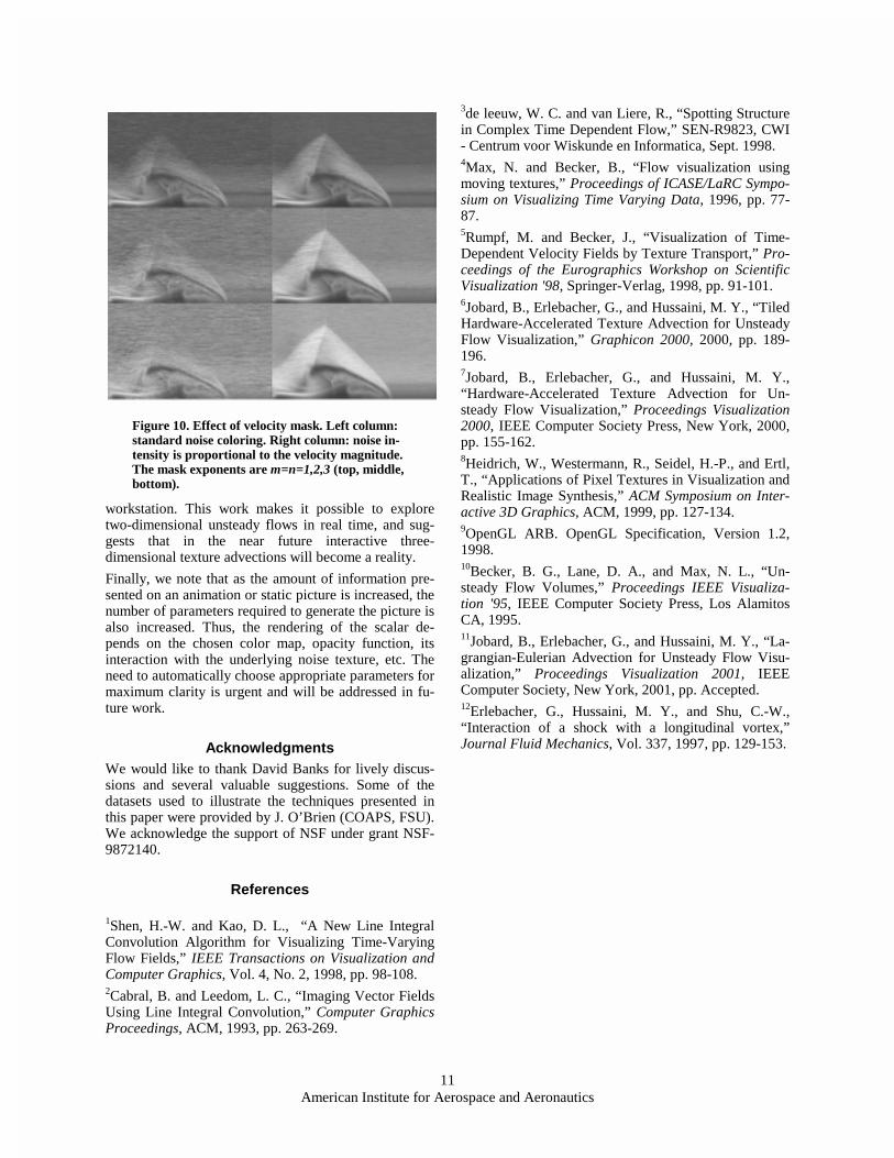
The opacity masking function is defined by two parame-ters: m controls the relation between opacity and noise intensity, and n controls the effect of velocity magni-tude on opacity. In Figure 10, we show the effect of the mask on the flow at a fixed time. The same scalar func-tion has also been superimposed. In the left column,

0n = . The opacity is only determined by the noise intensity. Although the length of the streaks that result from the temporal blending of successive temporal im-ages is proportional to the velocity magnitude, the con-trast between regions of low and high velocity is not very strong. The transparency mask acts as a form of

anisotropic and locally homogeneous dithering. The contrast becomes stronger as m is increased from 1 (top) to 3 (bottom). Increased contrast is achieved by combining 1m = with a modulation of opacity with velocity magnitude. As expected, the contrast becomes sharper as n increases from 1 (top) to 3 (bottom).

Concluding Remarks This paper describes an algorithm to visualize time-dependent flows based on an original per-pixel Lagran-gian-Eulerian Advection approach. A noise image is advected from a time step to the next. The color of every pixel in the current image is determined in two steps. A dense collection of particles (one per pixel) is first integrated backward in time for a fixed time inter-val (Lagrangian phase) to determine their positions in the previous frame. The color at these positions deter-mines the color of each pixel in the current frame (Eule-rian phase). We describe how to seamlessly handle regions where the flow enters the physical domain. A temporal filter is applied to successive images to intro-duce a good level of spatio-temporal correlation. Thus, every still frame represents the instantaneous structure of the flow, whereas an animated sequence of frames reveals the motion of a dense collection of particles released into the flow. When necessary, spatial correla-tion is enhanced through a fast LIC algorithm. A post-processing filter is described to control the contrast be-tween regions of high and low velocity magnitude. Transparency makes it possible to view a background image through the flow; which leads to our current in-vestigation into multiple layer texture advection. We have demonstrated the efficiency of the algorithm on a variety of computers, including a multiprocessor

Figure 9. Interaction of a planar shock with a lon-gitudinal vortex time sequence. Cubic opacity mask. Gray intensity is proportional to velocity magnitude.


workstation. This work makes it possible to explore two-dimensional unsteady flows in real time, and sug-gests that in the near future interactive three-dimensional texture advections will become a reality.

Finally, we note that as the amount of information pre-sented on an animation or static picture is increased, the number of parameters required to generate the picture is also increased. Thus, the rendering of the scalar de-pends on the chosen color map, opacity function, its interaction with the underlying noise texture, etc. The need to automatically choose appropriate parameters for maximum clarity is urgent and will be addressed in fu-ture work.

Acknowledgments We would like to thank David Banks for lively discus-sions and several valuable suggestions. Some of the datasets used to illustrate the techniques presented in this paper were provided by J. O’Brien (COAPS, FSU). We acknowledge the support of NSF under grant NSF-9872140.

References

1Shen, H.-W. and Kao, D. L., “A New Line Integral Convolution Algorithm for Visualizing Time-Varying Flow Fields,” IEEE Transactions on Visualization and Computer Graphics, Vol. 4, No. 2, 1998, pp. 98-108. 2Cabral, B. and Leedom, L. C., “Imaging Vector Fields Using Line Integral Convolution,” Computer Graphics Proceedings, ACM, 1993, pp. 263-269.

3de leeuw, W. C. and van Liere, R., “Spotting Structure in Complex Time Dependent Flow,” SEN-R9823, CWI - Centrum voor Wiskunde en Informatica, Sept. 1998. 4Max, N. and Becker, B., “Flow visualization using moving textures,” Proceedings of ICASE/LaRC Sympo-sium on Visualizing Time Varying Data, 1996, pp. 77-87. 5Rumpf, M. and Becker, J., “Visualization of Time-Dependent Velocity Fields by Texture Transport,” Pro-ceedings of the Eurographics Workshop on Scientific Visualization '98, Springer-Verlag, 1998, pp. 91-101. 6Jobard, B., Erlebacher, G., and Hussaini, M. Y., “Tiled Hardware-Accelerated Texture Advection for Unsteady Flow Visualization,” Graphicon 2000, 2000, pp. 189-196. 7Jobard, B., Erlebacher, G., and Hussaini, M. Y., “Hardware-Accelerated Texture Advection for Un-steady Flow Visualization,” Proceedings Visualization 2000, IEEE Computer Society Press, New York, 2000, pp. 155-162. 8Heidrich, W., Westermann, R., Seidel, H.-P., and Ertl, T., “Applications of Pixel Textures in Visualization and Realistic Image Synthesis,” ACM Symposium on Inter-active 3D Graphics, ACM, 1999, pp. 127-134. 9OpenGL ARB. OpenGL Specification, Version 1.2, 1998. 10Becker, B. G., Lane, D. A., and Max, N. L., “Un-steady Flow Volumes,” Proceedings IEEE Visualiza-tion '95, IEEE Computer Society Press, Los Alamitos CA, 1995. 11Jobard, B., Erlebacher, G., and Hussaini, M. Y., “La-grangian-Eulerian Advection for Unsteady Flow Visu-alization,” Proceedings Visualization 2001, IEEE Computer Society, New York, 2001, pp. Accepted. 12Erlebacher, G., Hussaini, M. Y., and Shu, C.-W., “Interaction of a shock with a longitudinal vortex,” Journal Fluid Mechanics, Vol. 337, 1997, pp. 129-153.

Figure 10. Effect of velocity mask. Left column: standard noise coloring. Right column: noise in-tensity is proportional to the velocity magnitude. The mask exponents are m=n=1,2,3 (top, middle, bottom).

real-time visualization of unsteady vector …gerlebacher/home/publications/reno_2002... ·...

Documents