JHEP01(2012)028

Published for SISSA by Springer

Received: November 2, 2011

Accepted: December 16, 2011

Published: January 9, 2012

Realizability of the Lorentzian (n, 1)-simplex

Kyle Tate and Matt Visser

School of Mathematics, Statistics, and Operations Research, Victoria University of Wellington,

PO Box 600, Wellington 6140, New Zealand

E-mail: kyle.tate@msor.vuw.ac.nz, matt.visser@msor.vuw.ac.nz

Abstract: In a previous article [JHEP 11 (2011) 072; arXiv:1108.4965] we have de-

veloped a Lorentzian version of the Quantum Regge Calculus in which the significant

differences between simplices in Lorentzian signature and Euclidean signature are crucial.

In this article we extend a central result used in the previous article, regarding the realiz-

ability of Lorentzian triangles, to arbitrary dimension. This technical step will be crucial

for developing the Lorentzian model in the case of most physical interest: 3+1 dimensions.

We first state (and derive in an appendix) the realizability conditions on the edge-

lengths of a Lorentzian n-simplex in total dimension n = d + 1, where d is the number

of space-like dimensions. We then show that in any dimension there is a certain type of

simplex which has all of its time-like edge lengths completely unconstrained by any sort of

triangle inequality. This result is the d+ 1 dimensional analogue of the 1 + 1 dimensional

case of the Lorentzian triangle.

Keywords: Models of Quantum Gravity, Lattice Models of Gravity

ArXiv ePrint: 1110.5694

c© SISSA 2012 doi:10.1007/JHEP01(2012)028

JHEP01(2012)028

Contents

1 Introduction 1

2 Realizability of generic simplices 2

3 Realizability of the Lorentzian (n, 1) simplex 3

4 Constraints on the other Lorentzian (l, k) simplices 7

5 Conclusions 8

A Lorentzian-signature Cayley-Menger determinant 9

1 Introduction

In the formulation of Lorentzian Fixed Triangulations (LFT) which we developed in ref-

erence [1], an important geometrical fact about a certain type of Lorentzian 2-simplex

(Lorentzian triangle) in 1 + 1 dimensions is exploited: All three of its edge-lengths, one

space-like and two time-like, are completely unconstrained by any form of the triangle in-

equalities. This is in stark contrast to the situation in Euclidean signature. In particular,

the absence of any triangle inequality constraints allowed for the explicit demonstration,

essentially dependent on the difference in configuration spaces, that the Euclidean and

Lorentzian Quantum Regge Calculus are not simply related theories — that is, they are

not related by a naive “Wick Rotation”. (See references [2–4] for additional background.)

In the case of quantum field theories defined on flat Minkowski space there are rigorous

mathematical theorems relating the Euclidean-signature Osterwalder-Schrader axioms to

the equivalent Lorentzian-signature Wightman axioms, so in that situation the choice of

whether to work in Euclidean signature or Lorentzian signature can be based on technical

convenience. For quantum gravity no such formal axiom structure exists, and there is no

equivalent theorem of this nature. That is, there is no physics reason to expect candidate

models for Euclidean quantum gravity and Lorentzian quantum gravity to be the same

theory — and in fact the difference in classical configuration spaces indicates that in (at

least in 1+1 dimensions) they cannot be the same theory.

In this current article, we will demonstrate that in any dimension n = d + 1 there

is a Lorentzian n-simplex which has all of its time-like edge lengths unconstrained. This

will be important for formulating LFT in n dimensions, as it implies that the non-trivial

distinction between the Lorentzian and Euclidean theories holds in any dimension. We also

discuss the origin of constraints on the time-like edges of the remaining simplices which are

not of the specific type mentioned above.

– 1 –

JHEP01(2012)028

2 Realizability of generic simplices

An n-simplex (in either Euclidean or Lorentzian signature), which we will denote by the

symbol < 012 · · ·n >, consists of n+ 1 vertices connected by 12n(n+ 1) edges. Given a set

of 12n(n+ 1) squared edge lengths {D2

ij | i, j = 0, · · · , n}, a simplex is called “realizable” if

one can find a linear imbedding of the n + 1 vertices into flat space/spacetime such that

the squared distance from vertex i to vertex j is given by the specified D2ij .

• For a Euclidean n-simplex this corresponds to finding a linear imbedding in the Rn

Euclidean space, where the distance is given by the standard Euclidean inner product

(D2ij = (D2

E)ij).

• For a Lorentzian n-simplex this corresponds to finding a linear imbedding in the Rd,1

Minkowski space with n = d+ 1, where the distance is given by the Minkowski inner

product (D2ij = (D2

L)ij).

For a Euclidean n-simplex a necessary and sufficient condition for it to be realizable in

this sense is for its Cayley-Menger determinant (and appropriate minors) to have the

appropriate (dimension dependent) sign. This is equivalent to the statement that the

square of the volume be positive [5–8], both for the simplex itself and for an appropriate

selection of its sub-simplices.

The so-called Cayley-Menger determinant is the determinant of the (n+ 2)× (n+ 2)

matrix E2ab which has entries E2

ij = 〈~vi−~vj , ~vi−~vj〉 = (D2E)ij for i, j = 0, · · · , n, and which

is augmented by an additional row and column with entries given by En+1,n+1 = 0 and

Ei,n+1 = En+1,j = 1. That is

E2ab =

[(D2

E)ij 1i

1j 0

]. (2.1)

We will call this matrix the Cayley-Menger matrix. The proportionality factor occurring

in the volume formula is combinatorial in nature, and depends on the dimension n. The

volume of the simplex is given by:

(Vn)2E =(−1)n+1

2n(n!)2|E2

ab|. (2.2)

The distance matrix (DE)2ij represents a realizable simplex only if

sign(|E2

ab|)

= (−1)n+1, (2.3)

so that the volume is real.

As stated in [1] there is an analogous Cayley-Menger determinant and volume formula

for the Lorentzian n-simplex, with Euclidean distances replaced by Lorentzian distances in

the Lorentzian Cayley-Menger matrix L2ab. That is:

L2ab =

[(D2

L)i,j 1i

1j 0

]. (2.4)

– 2 –

JHEP01(2012)028

The corresponding Lorentzian Cayley-Menger determinant formula for the volume is

(Vn)2L =(−1)n

2n(n!)2|L2ab|. (2.5)

The squared volume must again be positive for the simplex to be realizable in Rd,1. Deriving

this result is straightforward, and is very similar to the usual derivation in Euclidean space.

We will therefore relegate the details to appendix A. We should point out that the derivation

presented in that appendix is “direct” — the derivation does not mention the term “Wick

rotation”, nor does it need any such concept. In principle equation (2.5) describes a function

of the 12n(n+ 1) edge lengths whose positivity tells one everything that one needs to know

about the realizability of Lorentzian n-simplices.

However, its compact form obscures the main result of this article: There is a special

class of Lorentzian simplices for which, (once the spacelike edges have been chosen in an

appropriate manner), the function is always positive for any arbitrary choice of the time-like

edge lengths. That is: those edge lengths which have (D2L)ij < 0 can be chosen arbitrarily.

3 Realizability of the Lorentzian (n, 1) simplex

In both LFT [1] and CDT [9–13], the class of Lorentzian simplices one considers are the

(l, k) simplices (where l + k = n+ 1). These are simplices which have a (l − 1)-Euclidean

simplex in one space-like hypersurface, connected in “time” to a Euclidean (k− 1)-simplex

in the subsequent space-like hypersurface. Note that there are then

l(l − 1)

2+k(k − 1)

2=

(n+ 1)(n− 2k) + 2k2

2(3.1)

space-like edges and

kl = k(n+ 1− k) (3.2)

time-like edges in the simplex. The simplex which in n dimensions has all of its n time-like

edge lengths completely unconstrained by triangle inequalities is the (n, 1) simplex. (See

for example figure 1.)

Specifically, the (n, 1) simplex contains a Euclidean (n−1)-simplex sitting in an n−1 =

d dimensional space-like hypersurface, which is connected by n time-like edge lengths to

a single vertex in the subsequent n − 1 dimensional space-like hypersurface. We assume

that the Euclidean (n − 1)-simplex < 01 · · · (n − 1) > is realizable, that is we can find

coordinates xµi for the i = 0, 1, · · · , n− 1 vertices with xµ = (x1, x2, · · · , xn) where in this

article we will denote the time coordinate by t = xn. Without loss of generality we can

choose our coordinate system such that the vertex < 0 > is at the origin, then we can

define the vectors ~v1, ~v2, · · · , ~vn−1 to be the edges < 01 >, < 02 >, · · · , < 0(n−1) >. Since

these vectors span a space-like hypersurface, we can choose our coordinate system so that

xni = ti = 0. In order for the (n, 1) simplex to be realizable, with time-like edge lengths

given by

T 2i = 〈~vn − ~vi, ~vn − ~vi〉 < 0, (3.3)

– 3 –

JHEP01(2012)028

< 1 >

< 0 >< 2 >

< 3 >

Figure 1. The (3,1) tetrahedron in 2+1 dimensions. The < 012 > 2-simplex is a Euclidean triangle.

The < 30 >, < 31 >, and < 32 > 1-simplices are time-like edges whose lengths are unconstrained

by any triangle inequalities.

where ~vn is the vector from the origin to the vertex < n >, we must be able to find

coordinates xµn such that the following nonlinear equations hold:

ηµν(xn − x0)µ (xn − x0)ν = −T 20 ,

ηµν(xn − x1)µ (xn − x1)ν = −T 21 ,

ηµν(xn − x2)µ (xn − x2)ν = −T 22 ,

...

ηµν(xn − xn−1)µ (xn − xn−1)

ν = −T 2n−1. (3.4)

We have chosen a coordinate system where xµ0 = 0, and we have boosted in the space-like

hyper-surface so that ∀i we have xni = 0. We can make use of the rotational freedom in

the space-like hypersurface to choose xji = 0 for i < j, i, j = 0, · · · , n− 1. That is:

x1 = (x11, 0, 0, · · · , 0),

x2 = (x12, x22, 0, · · · , 0),

x3 = (x13, x23, x

33, · · · , 0),

...

xn−1 = (x1n−1, x2n−1, x

3n−1, · · · , xn−1

n−1, 0). (3.5)

In contrast the nth vector

xn = (x1n, x2n, x

3n, · · · , xn−1

n , xnn) (3.6)

has no a priori zeros. Note that the components xji form a lower-triangular matrix so the

n× n determinant |xji | is simply∏i x

ii. With these coordinate choices, the equations (3.4)

– 4 –

JHEP01(2012)028

become:

(x1n)2 + (x2n)2 + (x3n)2 · · ·+ (xn−1n )2 − (xnn)2 = −T 2

0 ,

(x1n − x11)2 + (x2n)2 + (x3n)2 · · ·+ (xn−1n )2 − (xnn)2 = −T 2

1 ,

(x1n − x12)2 + (x2n − x22)2 + (x3n)2 · · ·+ (xn−1n )2 − (xnn)2 = −T 2

2 , (3.7)

...

(x1n − x1n−1)2 + (x2n − x2n−1)

2 + (x3n − x3n−1)2 · · ·+ (xn−1

n − xn−1n−1)

2 − (xnn)2 = −T 2n−1.

As long as the Euclidean sub-simplex is non-degenerate, which by the above requires that

∀i ∈ {1, . . . , n− 1} we have xii 6= 0, this system of equations can be inverted recursively:

x1n =(x11)

2 + T 21 − T 2

0

2x11,

x2n =(x22)

2 − 2x1nx12 + (x12)

2 + T 22 − T 2

0

2x22,

x3n =(x33)

2 − 2x2nx23 + (x23)

2 − 2x1nx13 + (x13)

2 + T 23 − T 2

0

2x33, (3.8)

...

xnn = t = ±√

(x1n)2 + (x2n)2 + (x23)2 + · · ·+ (xn−1

n )2 + T 20 .

That the system of equations (3.7) always has two distinct solutions (related by reflection

through t = 0) is best understood by realizing that it is equivalent to the fact that the n

hyperboloids defined in equations (3.7) have two intersections, one in the joint intersection

of the future light cones of the vertices < 0 >, · · · , < n − 1 >, and one in the joint

intersection of the past light cones.

Thus we can state the main result of this article: In any dimension n = d+ 1, d > 0,

there exists a Lorentzian n-simplex denoted (n, 1) which, provided its Euclidean sub-simplex

is realizable, has all its n time-like edge lengths completely unconstrained.

The result can also be understood by directly examining the Cayley-Menger determi-

nant (2.5). This is because, for the (n, 1) simplex all of the time-like edge lengths are only

in one column (row). Suitably permuting indices one has

(V(n,1)

)2=

(−1)n

2n(n!)2det(L2) =

(−1)n

2n(n!)2

∣∣∣∣∣ E2 ~T

~T T 0

∣∣∣∣∣ . (3.9)

Here E2 is the reduced Cayley-Menger matrix for the d = (n − 1) dimensional Euclidean

sub-simplex, and~T =

(1,−T 2

0 ,−T 21 , · · · ,−T 2

n−1

)T. (3.10)

Let U be the (n+ 1)× (n+ 1) identity matrix, augmented with an extra column and row,

Un+1,i = ~αTi , Ui,n+1 = 0, and Un+1,n+1 = β, where the ~α and β are at this stage unspecified

numbers:

U =

(I 0

~αT β

). (3.11)

– 5 –

JHEP01(2012)028

Examine the matrix equation:

L2 = UL2UT , (3.12)

where L2 is the Cayley-Menger matrix of the Euclidean (n− 1)-simplex, augmented with

an extra row and column, L2n+1,n+1 = 1, L2

n+1,i = L2i,n+1 = 0:

L2 =

(E2 0

0 1

). (3.13)

Solving equation (3.12) is identical to solving the vector equation

E2~α = −β ~T , (3.14)

and the scalar equation

β~αT ~T = 1. (3.15)

Since we are assuming that the Euclidean sub-simplex is realizable, (and in particular non-

degenerate), E2 is invertible and there is a unique solution to equation (3.14) for ~α in terms

of β and the T 2i :

~α = −β(E2)−1 ~T . (3.16)

Assuming that ~T T (E2)−1 ~T 6= 0, (we shall soon see that ~T T (E2)−1 ~T = −2t2), the scalar

equation has solution

β2 = − 1

~T T (E2)−1 ~T, (3.17)

where we have used the fact that E2 = (E2)T . Note that det(U) = β, and provided β 6= 0,

then U is invertible. Suppose this is the case, then we can rewrite equation (3.9) as(V(n,1)

)2=

(−1)n

2n(n!)2det[(U−1)T L2U−1

]=

(−1)n

2n(n!)2(det[UTU ]

)−1det[L2]

=(−1)n

2n(n!)2(det[UTU ]

)−1det[E2]

=1

2

1

β21

n2(−1)(n−1)+1

2n−1((n− 1)!)2det[E2]

=1

2β2 n2(VE)2n−1, (3.18)

where, as stated above, E2 is the (n+ 1, n+ 1) cofactor of L2, which is the Cayley-Menger

matrix for the Euclidean (n− 1)-simplex, and in the last step we have used equation (2.2).

Finally, using the fact that the volume of a simplex can always be written as

Vn =1

nVn−1 h, (3.19)

where h is the perpendicular distance from the (n− 1)-sub-simplex to the last vertex, and

in light of equation (3.8) we have:(V(n,1)

)2=t2

n2(VE)2n−1. (3.20)

– 6 –

JHEP01(2012)028

S1

T2T1T3

S2

T4

Figure 2. The (2,2) tetrahedron with edge lengths explicitly displayed. S1 and S2 are space-like,

whereas T1, T2, T3, and T4 are time-like.

Thus we can identify

β =1√2 t. (3.21)

So we explicitly see that the positivity of the (n, 1) Cayley-Menger determinant reduces to

the realizability condition on the Euclidean sub-simplex, plus the existence of a nonzero

solution for β, or equivalently t. This existence of this solution is guaranteed by (3.8).

As mentioned above, this decomposition can only be done for the (n, 1) simplex; for the

other (l, k) simplices the time-like edge lengths get mixed up in columns (rows) with the

space-like edge lengths.

4 Constraints on the other Lorentzian (l, k) simplices

To understand why the constraints on the (n, 1) simplex are straightforwardly simple, in

contrast to those for the other (l, k) simplices, it is instructive to consider the first dimension

where this distinction arises: n = 2 + 1. In dimension 2 + 1 there are two simplices that

need to be considered: The elementary (3, 1) simplex of figure 1 and the more complex

(2, 2) simplex of figure 2.

As stated above, the simplicity of the (3, 1) simplicial constraints can be seen to be

a result of the fact that given a Euclidean triangle in a space-like hyper-surface the three

hyperboloids, defined as the set of points for which the time-like distance from each vertex

is fixed to a certain value, always have precisely two intersections: one in the forward

light cone and one in the past lightcone. For the (2, 2) simplex with edge lengths given by

S1, S2, T1, T2, T3, T4 the fact that these edge legths may be non-realizable can be understood

as follows: First, given S1, T1, T2 we can always choose the coordinate system where the

vertices are at (x, y, t) = (−S1/2, 0,−S1/2), (S1/2, 0,−S1/2), and (X, 0, τ) respectively,

where

τ =1

2S1

(√(S2 + [T1 − T2]2)(S2

1 + [T1 + T2]2)− S21

), (4.1)

X =1

2S1

(T 22 − T 2

1

). (4.2)

Then, given some S2, T3, and T4, we need to find coordinates (x, y, t) such that we have

a realizable (2, 2) simplex. For it to be realizable, the point (x, y, t) must be inside the

– 7 –

JHEP01(2012)028

intersection of the light cones of the first two space-like vertices (call that region T12 = T1∩T2), and outside of the lightcone of the third vertex (call that region S3 = (T3)c = R2,1\T3).Thus we have:

T12 =

{(t, x, y)

∣∣∣∣ (|x|+ S12

)2

+ y2 −(t+

S12

)2

≤ 0

}; (4.3)

S3 ={

(t, x, y)∣∣ (x−X)2 + y2 − (t− τ)2 > 0

}; (4.4)

R = T12 ∩ S3. (4.5)

Thus we see that the constraints on the (2, 2) simplex have their origin in the question of

whether or not there exists a point (x, y, t) in the region (4.5) such that the three remaining

edges (one space-like and two time-like) have length S2, T3 and T4.

Of course this is equivalent to the fact, pointed out in reference [1], that if one considers

the time-like edge lengths as vectors directed from one of the space-like hyper-surface to

the other, then ~T1 + ~T3 = ~T2 + ~T4. This is the same as stating that given ~T1 and ~T2 the

other two time-like edges must be such that ~T1− ~T4 and ~T2− ~T4 are space-like, that is they

must be inside the region (4.5).

Turning to the physically interesting case of 3 + 1 dimensions, there are only two

distinct (l, k) simplices: The (4, 1) simplex, which by the results of this article has no con-

straints on its time-like edge lengths, and the (3, 2) simplex. This (3, 2) simplex in 3+1

dimensions will be constrained in a similar fashion to the (2, 2) simplex in 2+1 dimensions.

Note that the (3, 2) simplex contains one Euclidean triangle, nine Lorentzian triangles, two

(3, 1) tetrahedra and three (2, 2) tetrahedra. Each of these sub-simplices must be realizable

and hence, in addition to a standard Euclidean constraint, (that on the Euclidean trian-

gle), there will also be constraints on the six time-like edge lengths arising from the (2, 2)

tetrahedral sub-simplices. Note however that in general for a simplex to be realizable it is

necessary but not sufficient that its sub-simplices be realizable. That is to say, one should

expect that in addition to the constraints arising from the (2, 2) tetrahedron, there will

now be further constraints arising from the 3 + 1 dimensional Cayley-Menger determinant.

Nevertheless, it is safe to say that for certain choices of time-like edges the Lorentzian (3, 2)

simplex will not be realizable, which stands in contrast to the Lorentzian (4, 1) simplex.

5 Conclusions

In this article we have shown that in any dimension n = d+ 1, where d > 0, there exists a

Lorentzian n-simplex denoted (n, 1) which, provided its Euclidean sub-simplex is realizable,

has its n time-like edge lengths completely unconstrained. This was claimed in reference [1]

without explicit proof, and this article has served as verification of that claim. As a result

we have shown that in all dimensions, the geometry of simplices in Lorentzian signature

can be surprisingly and significantly different from their geometry in Euclidean signature.

This observation is of particular relevance for simplicial models of quantum gravity

in that it implies that the configuration space for path integrals over simplicial manifolds,

that is the set of edge lengths for which every simplex in the manifold is realizable, de-

pends on whether one’s model is formulated in Euclidean or Lorentzian signature. This

– 8 –

JHEP01(2012)028

difference further strengthens the notion, first encountered in the formulation of CDTs and

further developed in reference [1], that simplicial approaches to quantum gravity should

be developed directly in Lorentzian signature, rather than first in Euclidean signature and

then trying to Wick rotate to relate the results to Lorentzian signature.

A Lorentzian-signature Cayley-Menger determinant

Suppose we have a realizable n-simplex in n = d + 1 Minkowski space < 012 . . . n >,

with squared edge lengths (D2L)ij . By realizability, we mean that given the n + 1 edge

lengths there exists a linear embedding of the simplex in d + 1 space, that is we can find

coordinates xµi = (x1i , . . . , xdi , ti) for each vertex i = 0, . . . , n (where we identify ti = xni )

such that (D2L)ij = 〈xi−xj , xi−xj〉. If this holds, and we place the vertex 0 at the origin,

then exactly as if this were a Euclidean simplex, the volume is given by

Vn =1

n!detXij , (A.1)

where Xij = xji . Let us now use this result to derive the Lorentzian-signature Cayley-

Menger formula for Lorentzian volume. We have:

Vn =1

n!

∣∣∣∣∣∣∣x11 · · · xn1...

. . ....

x1n · · · xnn

∣∣∣∣∣∣∣ . (A.2)

We can move away from referencing the origin by subtracting the coordinates of xµ0 :

Vn =1

n!

∣∣∣∣∣∣∣x11 − x10 · · · xn1 − xn0

.... . .

...

x1n − x10 · · · xnn − xn0

∣∣∣∣∣∣∣ . (A.3)

We can add the following column and row without changing the volume, changing the

determinant by (−1)n+1:

Vn =(−1)n+1

n!

∣∣∣∣∣∣∣∣∣∣1 x11 − x10 · · · xn1 − xn0...

.... . .

...

1 x1n − x10 · · · xnn − xn01 0 · · · 0

∣∣∣∣∣∣∣∣∣∣. (A.4)

Adding xi0 times the first column to the ith column does not change the determinant:

Vn =(−1)n+1

n!

∣∣∣∣∣∣∣∣∣∣1 x11 · · · xn1...

.... . .

...

1 x1n · · · xnn1 x10 · · · xn0

∣∣∣∣∣∣∣∣∣∣. (A.5)

– 9 –

JHEP01(2012)028

Multiply the last column by −1:

Vn =(−1)n

n!

∣∣∣∣∣∣∣∣∣∣1 x11 · · · −xn1...

.... . .

...

1 x1n · · · −xnn1 x10 · · · −xn0

∣∣∣∣∣∣∣∣∣∣, (A.6)

then multiply each side of (A.6) by the determinant of the transpose of (A.5):

V 2n =

−1

(n!)2

∣∣∣∣∣∣∣∣∣∣1 x11 · · · −xn1...

.... . .

...

1 x1n · · · −xnn1 x10 · · · −xn0

∣∣∣∣∣∣∣∣∣∣

∣∣∣∣∣∣∣∣∣∣1 1 · · · 1

x11 · · · x1n x10...

.... . .

...

xn1 · · · xnn xn0

∣∣∣∣∣∣∣∣∣∣. (A.7)

Hence

V 2n =

−1

(n!)2

∣∣∣∣∣∣∣∣∣∣1 + 〈x1, x1〉 1 + 〈x1, x2〉 · · · 1 + 〈x1, x0〉

......

. . ....

1 + 〈xn, x1〉 1 + 〈xn, x2〉 · · · 1 + 〈xn, x0〉1 + 〈x0, x1〉 1 + 〈x0, x2〉 · · · 1 + 〈x0, x0〉

∣∣∣∣∣∣∣∣∣∣, (A.8)

where 〈·, ·〉 is the Minkowski inner product. Now add the following rows and columns,

noting that they do not change the determinant:

V 2n =

−1

(n!)2

∣∣∣∣∣∣∣∣∣∣∣∣

1 1 · · · 1

0 1 + 〈x1, x1〉 · · · 1 + 〈x1, x0〉...

.... . .

...

0 1 + 〈xn, x1〉 · · · 1 + 〈xn, x0〉0 1 + 〈x0, x1〉 · · · 1 + 〈x0, x0〉

∣∣∣∣∣∣∣∣∣∣∣∣. (A.9)

Subtract the first row from every other row:

V 2n =

−1

(n!)2

∣∣∣∣∣∣∣∣∣∣∣∣

1 1 · · · 1

−1 〈x1, x1〉 · · · 〈x1, x0〉...

.... . .

...

−1 〈xn, x1〉 · · · 〈xn, x0〉−1 〈x0, x1〉 · · · 〈x0, x0〉

∣∣∣∣∣∣∣∣∣∣∣∣. (A.10)

The cofactor C11 of the top-left element is zero since:∣∣∣∣∣∣∣∣∣∣〈x1, x1〉 · · · 〈x1, x0〉

.... . .

...

〈xn, x1〉 · · · 〈xn, x0〉〈x0, x1〉 · · · 〈x0, x0〉

∣∣∣∣∣∣∣∣∣∣=

∣∣∣∣∣∣∣∣∣∣0 x11 · · · −xn1...

.... . .

...

0 x1n · · · −xnn0 x10 · · · −xn0

∣∣∣∣∣∣∣∣∣∣

∣∣∣∣∣∣∣∣∣∣0 0 · · · 0

x11 · · · x1n x10...

.... . .

...

xn1 · · · xnn xn0

∣∣∣∣∣∣∣∣∣∣= 0. (A.11)

– 10 –

JHEP01(2012)028

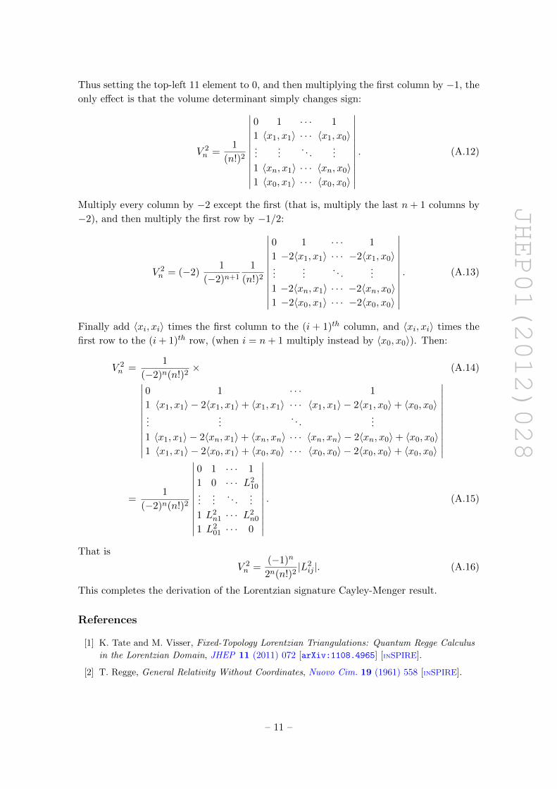
Thus setting the top-left 11 element to 0, and then multiplying the first column by −1, the

only effect is that the volume determinant simply changes sign:

V 2n =

1

(n!)2

∣∣∣∣∣∣∣∣∣∣∣∣

0 1 · · · 1

1 〈x1, x1〉 · · · 〈x1, x0〉...

.... . .

...

1 〈xn, x1〉 · · · 〈xn, x0〉1 〈x0, x1〉 · · · 〈x0, x0〉

∣∣∣∣∣∣∣∣∣∣∣∣. (A.12)

Multiply every column by −2 except the first (that is, multiply the last n+ 1 columns by

−2), and then multiply the first row by −1/2:

V 2n = (−2)

1

(−2)n+1

1

(n!)2

∣∣∣∣∣∣∣∣∣∣∣∣

0 1 · · · 1

1 −2〈x1, x1〉 · · · −2〈x1, x0〉...

.... . .

...

1 −2〈xn, x1〉 · · · −2〈xn, x0〉1 −2〈x0, x1〉 · · · −2〈x0, x0〉

∣∣∣∣∣∣∣∣∣∣∣∣. (A.13)

Finally add 〈xi, xi〉 times the first column to the (i + 1)th column, and 〈xi, xi〉 times the

first row to the (i+ 1)th row, (when i = n+ 1 multiply instead by 〈x0, x0〉). Then:

V 2n =

1

(−2)n(n!)2× (A.14)∣∣∣∣∣∣∣∣∣∣∣∣

0 1 · · · 1

1 〈x1, x1〉 − 2〈x1, x1〉+ 〈x1, x1〉 · · · 〈x1, x1〉 − 2〈x1, x0〉+ 〈x0, x0〉...

.... . .

...

1 〈x1, x1〉 − 2〈xn, x1〉+ 〈xn, xn〉 · · · 〈xn, xn〉 − 2〈xn, x0〉+ 〈x0, x0〉1 〈x1, x1〉 − 2〈x0, x1〉+ 〈x0, x0〉 · · · 〈x0, x0〉 − 2〈x0, x0〉+ 〈x0, x0〉

∣∣∣∣∣∣∣∣∣∣∣∣

=1

(−2)n(n!)2

∣∣∣∣∣∣∣∣∣∣∣∣

0 1 · · · 1

1 0 · · · L210

......

. . ....

1 L2n1 · · · L2

n0

1 L201 · · · 0

∣∣∣∣∣∣∣∣∣∣∣∣. (A.15)

That is

V 2n =

(−1)n

2n(n!)2|L2ij |. (A.16)

This completes the derivation of the Lorentzian signature Cayley-Menger result.

References

[1] K. Tate and M. Visser, Fixed-Topology Lorentzian Triangulations: Quantum Regge Calculus

in the Lorentzian Domain, JHEP 11 (2011) 072 [arXiv:1108.4965] [INSPIRE].

[2] T. Regge, General Relativity Without Coordinates, Nuovo Cim. 19 (1961) 558 [INSPIRE].

– 11 –

JHEP01(2012)028

[3] R.M. Williams, Recent progress in Regge calculus, Nucl. Phys. Proc. Suppl. 57 (1997) 73

[gr-qc/9702006] [INSPIRE].

[4] H.W. Hamber and R.M. Williams, Discrete Wheeler-DeWitt Equation, Phys. Rev. D 84

(2011) 104033 [arXiv:1109.2530] [INSPIRE].

[5] L.M. Blumenthal, Theory and Applications of Distance Geometry, Oxford University Press,

Oxford U.K. (1953).

[6] D.M.Y. Sommerville, An Introduction to the Geometry of n Dimensions, Dover, New York

U.S.A. (1958).

[7] A. Cayley, On a theorem in the geometry of position, Cambridge Math. J. 2 (1841) 267.

[8] K. Menger, Untersuchungen uber allegemeine Metrik, Math. Annal. 100 (1928) 47.

[9] J. Ambjørn and R. Loll, Nonperturbative Lorentzian quantum gravity, causality and topology

change, Nucl. Phys. B 536 (1998) 407 [hep-th/9805108] [INSPIRE].

[10] R. Loll, Discrete Lorentzian quantum gravity, Nucl. Phys. Proc. Suppl. 94 (2001) 96

[hep-th/0011194] [INSPIRE].

[11] J. Ambjørn, J. Jurkiewicz and R. Loll, Dynamically triangulating Lorentzian quantum

gravity, Nucl. Phys. B 610 (2001) 347 [hep-th/0105267] [INSPIRE].

[12] J. Ambjørn, J. Jurkiewicz and R. Loll, Lattice quantum gravity - an update,

PoS(LATTICE2010)014 [arXiv:1105.5582] [INSPIRE].

[13] J. Ambjørn, S. Jordan, J. Jurkiewicz and R. Loll, A Second-order phase transition in CDT,

Phys. Rev. Lett. 107 (2011) 211303 [arXiv:1108.3932] [INSPIRE].

– 12 –