recent developments in the economics of price …else.econ.ucl.ac.uk/papers/uploaded/175.pdf ·...
TRANSCRIPT

P1: FCW/
CUNY595-04 Cuny535/Blundell 0 521 87152 2 Printer: cupusbw August 16, 2006 17:35 Char Count= 0
CHAPTER 4
Recent Developments in the Economicsof Price Discrimination∗
Mark Armstrong
Abstract
This paper surveys the recent literature on price discrimination. The focus is
on three aspects of pricing decisions: the information about customers avail-
able to firms; the instruments firms can use in the design of their tariffs; and
the ability of firms to commit to their pricing plans. Developments in market-
ing technology mean that firms often have access to more information about
individual customers than was previously the case. The use of this information
might be restricted by public policy towards customer privacy. Where it is not
restricted, firms may be unable to commit to how they use the information.
With monopoly supply, an increased ability to engage in price discrimination
will boost profit unless the firm cannot commit to its pricing policy. Likewise,
an enhanced ability to commit to prices will benefit a monopolist. With com-
petition, the effects of price discrimination on profit, consumer surplus and
overall welfare depend on the kinds of information and/or tariff instruments
available to firms. The ability to commit to prices may damage industry profit.
1 INTRODUCTION
This paper surveys, in a highly selective manner, recent progress that has beenmade in the economic understanding of price discrimination. One can say thatprice discrimination exists when two “similar” products with the same marginalcost are sold by a firm at different prices.1 There are many forms of price
* Much of this paper reflects joint work and discussions with John Vickers. In preparing this
paper I have greatly benefited from consulting the earlier and more comprehensive survey by
Lars Stole (2006), and the reader is referred to that survey for a more complete account of the
important contributions to this topic. Thanks for comments and criticisms are due to V. Bhaskar,
Richard Blundell, Jan Bouckaert, Yongmin Chen, Drew Fudenberg, Ken Hendricks (my excellent
discussant), Paul Klemperer, Marco Ottaviani, Barry Nalebuff, Pierre Regibeau, Patrick Rey, John
Thanassoulis, Frank Verboven, Nir Vulkan, Mike Waterson, and Mike Whinston. The support of
the Economic and Social Research Council (UK) is gratefully acknowledged.
1 Stigler (2004) suggests a definition that applies to a wider class of cases: Discrimination exists
when two similar products are sold at prices that are in different ratios to their marginal costs.
97
Cambridge Collections Online © Cambridge University Press, 2006

P1: FCW/
CUNY595-04 Cuny535/Blundell 0 521 87152 2 Printer: cupusbw August 16, 2006 17:35 Char Count= 0
98 Advances in Economics and Econometrics
discrimination, including: charging different consumers different prices for thesame good (third-degree price discrimination); making the marginal price de-pend on the number of units purchased (nonlinear pricing); making the marginalprice depend on whether other products are also purchased from the same firm(bundling); making the price depend on whether this is the first time a consumerhas purchased from the firm (introductory offers; customer “poaching”).
In broad terms, this paper is about what happens to profit and consumersurplus when firms use more ornate tariffs to sell their products. There are tworeasons why a firm might be able to tune its tariff more finely: It might obtainmore detailed information about its potential customers, or it might be able touse additional instruments in its tariff design.
A firm can become better informed about its potential customers if it pur-chases customer data from a marketing company or from another firm. It canuse this data to send personalized price offers to new customers (an exampleof third-degree price discrimination).2 Alternatively, a firm might keep recordsof its customers’ past purchases and use this information to update its futureprices or the range of products offered to those customers. Firms’ access tobetter information is affected by public policy towards consumer privacy (forinstance, whether firms are permitted to pass information about their customersto other firms). It is also constrained by a consumer’s ability to “anonymise”contact with firms and to pretend to be a new customer.
Examples of the use of more tariff instruments include: using two-part tar-iffs instead of linear prices; charging different identifiable consumer groupsdifferent prices instead of a common price; offering a discount if two productsare jointly purchased; or making the price for an item depend on whether acustomer has previously purchased similar items from the firm.3 Public policytowards price discrimination affects the range of instruments that firms can use.Firms are also constrained in their range of instruments by the possibility ofarbitrage and resale between consumers.
A third theme of the paper, in addition to the effects of more information andinstruments, is how the ability of firms to commit to their pricing plans affectsoutcomes. Recent advances in marketing techniques may mean that the com-mitment problem has become more severe. The finely tuned customer data that
(This definition makes more sense when discussing “versioning,”where slightly different versions
of a product – such as hardback and paperback books – are offered for sale at very different
prices.) Which of these definitions we use makes no difference for the purposes of this paper.
An alternative definition might be that price discrimination is present when a similar product
is sold to different consumers at different prices. However, this definition rules out cases of
“intra-personal” discrimination, which are sometimes relevant, as discussed in section 4.1 below.2 See Taylor (2004, section 1) for a summary of the market for customer information. For instance,
he reports that a good customer mailing list can sell for millions of dollars on its own.3 Pure bundling – where two products are made available only as a joint purchase – is not a more
ornate tariff compared to separable prices, but rather just a different kind of tariff. However,
mixed bundling, where individual products as well as the bundle are offered for sale, is a more
ornate tariff compared to either pure bundling or separable prices.
Cambridge Collections Online © Cambridge University Press, 2006

P1: FCW/
CUNY595-04 Cuny535/Blundell 0 521 87152 2 Printer: cupusbw August 16, 2006 17:35 Char Count= 0
Recent Developments in the Economics of Price Discrimination 99
firms often possess permits the use of personalized prices. Such prices are often“secret” rather than public, and it is unlikely that firms can commit to such prices.Moreover, even if firms could commit, the complexity of the linkages betweenconsumer actions and future prices may be too complicated for many consumersto comprehend. A related theme is the impact of consumer naivete or sophisti-cation on firms’ policies. Most forms of personalised pricing make a customer’sfuture prices depend upon her past actions, often in a way that is not explicitlystated by firms. Sophisticated consumers – or consumers who have been activein a market for some time – may be able to predict the effect their actions willhave on their subsequent deals, and adjust their behavior accordingly. Naive con-sumers – or consumers in a new market – may not adequately take this linkageinto account, however, and firms may be in a position to exploit this myopia.4
A summary of the main results presented in the paper is as follows. Withmonopoly supply, except when commitment problems arise, the use of moreornate tariffs must lead to higher profits. When the firm has access to more de-tailed information about its customers or can use a wider range of instrumentsin its tariff, it can do no worse than before and generally it can do better. Withcompetition, though, the effects of using more ornate tariffs are less clear cut.In particular, in section 3 a Hotelling example is used to argue that the impact ofmore information on profits and prices depends crucially on the kind of informa-tion that becomes available. Some information will cause firms to make higherprofits in equilibrium, whereas other kinds of information will cause all pricesto fall compared to the situation with uniform pricing. An important factor forpredicting the impact of more information is whether firms agree about whichconsumers are “strong” and which are “weak.”5 If firms agree about the effect ofa specific kind of information on the incentive to set a higher or lower price (thecase of “best-response symmetry”), some prices will rise and others will fall,and profit will typically rise, when price discrimination is practiced. However,if firms obtain information about a consumer which suggests to one firm that itsprice to that consumer should rise and suggests to the other firm that its priceshould fall (“best-response asymmetry”), the outcome may well be that all pricesfall in equilibrium. In such cases, this competition-intensifying effect of pricediscrimination benefits all consumers. Finally, in section 3.4, the incentives offirms to acquire and to share information with rivals is considered. In cases ofbest-response symmetry, a firm typically wishes to acquire and to share its pri-vate information about consumers. With best-response asymmetry we show thata firm can sometimes be made worse off if it unilaterally acquires customer data.
The availability of an additional tariff instrument also has ambiguous ef-fects on profit and consumer surplus in oligopolistic settings (see section 4).Competing multiproduct firms often make less profit when they practice mixed
4 See Ellison (2006) for further discussion of the effects of (firm and consumer) bounded rationality.5 In the price discrimination literature, a market is said to be “strong” (“weak”) if a firm wishes
to raise (lower) its price there compared to the situation where it must charge a uniform price
across all markets.
Cambridge Collections Online © Cambridge University Press, 2006

P1: FCW/
CUNY595-04 Cuny535/Blundell 0 521 87152 2 Printer: cupusbw August 16, 2006 17:35 Char Count= 0
100 Advances in Economics and Econometrics
bundling than when they sell their products separately, while consumers ben-efit. In contrast, in a one-stop shopping framework where consumers buy allrelevant products from one firm, the effect of more ornate tariffs in competitivemarkets is often to boost profit and harm consumers. Unfortunately, the under-lying economic reasons for why some tariff instruments are profit-enhancing,while other instruments damage profit, is currently unclear.
In a dynamic context, a monopolist’s ability to commit to future pricesraises its profit, since this ability can only widen the range of tariffs that thefirm can offer (see section 2.2). With monopoly supply, profit is also higher ifconsumers are naive. Once a consumer has made a purchase, he typically revealshimself to be likely to purchase at the same price (or higher) subsequently,while consumers who do not initially purchase reveal that they are likely to beunwilling to pay a high price in the future. A firm that cannot commit (or whichfaces naive consumers) will price to these distinct consumer groups accordingly.In such situations, a policy that forbids price discrimination can act to restorecommitment power, to the detriment of consumers. The same pattern of pricesprevails in competitive settings, where firms price low to try to poach theirrival’s past customers. As with monopoly, consumers often benefit from thisform of price discrimination. However, in duopoly the ability to set long-termcontracts can be damaging to profit, and firms can also be worse-off if they facenaive consumers (see section 5).
The welfare effects of allowing price discrimination is ambiguous, bothwith monopoly and with oligopoly supply. Price discrimination can lead toefficient pricing (see section 2.1). When firms offer different prices to their loyalcustomers and to their rival’s previous customers this can make competitionmore intense, but it can also induce socially excessive switching between firms(section 5). By contrast, multiproduct firms might induce excessive loyalty, orone-stop shopping, when they offer bundling discounts (section 4.2). In a one-stop shopping framework, the effect of firms using more ornate tariffs is oftenwelfare-enhancing, at least in highly competitive markets. Price discriminationalso allows a firm to target price reductions more accurately at market segmentswhere competition is most intense. Doing so can harm rivals and deter entry,and as such can harm consumers compared to the case where discrimination isbanned (section 4.3). In sum, sensible policy towards price discrimination needsto be founded on a good economic understanding of the market in question.
2 MONOPOLY SUPPLY
2.1 Information and Instruments
With monopoly supply, the use of more ornate tariffs will boost profit, at least ifcommitment is not a problem. If the firm has access to more detailed informationabout its customers or to a wider range of tariff instruments, it can do no worsethan before and usually it can do better. In addition, the ability to commit tofuture prices can only enhance the monopolist’s profit, since the firm with suchan ability can always choose to implement the non-commitment price if it so
Cambridge Collections Online © Cambridge University Press, 2006

P1: FCW/
CUNY595-04 Cuny535/Blundell 0 521 87152 2 Printer: cupusbw August 16, 2006 17:35 Char Count= 0
Recent Developments in the Economics of Price Discrimination 101
chooses. (We will see later in the paper that these easy conclusions for monopolydo not easily carry over to competitive situations.)
In many cases, the efficiency losses caused by monopoly power are due tothe firm being unable to offer sufficiently ornate tariffs. In some circumstances,allowing firms to engage in price discrimination can implement efficient prices,in which case welfare is unambiguously improved. One familiar example isfirst-degree discrimination, where a monopolist has perfect information abouteach consumer’s valuation for its products and has the ability to set personal-ized prices. To be concrete, suppose there is a population of consumers, eachof whom wishes to consume a unit of the firm’s product. A consumer’s valu-ation for this unit is denoted v and this varies among consumers according tothe distribution function F(v). Suppose the firm has unit cost c. If price dis-crimination is not possible (e.g., because the firm does not have the necessaryinformation, cannot prevent arbitrage between consumers, or is not permitted toengage in discrimination), the firm will choose a uniform price p to maximizeprofit (p − c)(1 − F(p)). Clearly, this uniform price will be above cost, andtotal surplus is not maximized. (It is efficient to serve those consumers withv ≥ c, but only those with v ≥ p > c are served.) If the firm can observe eachconsumer’s v and is permitted to discriminate on that basis, it will charge thetype-v consumer p = v , provided this price covers its cost of supply. In otherwords, an efficient outcome is achieved. However, the firm appropriates theentire gains from trade and consumers are left with nothing.
There are also situations when price discrimination can lead to approxi-mately efficient prices, even when the monopolist has relatively little informa-tion about consumer tastes.6 A supermarket, say, supplies a large number ofproducts. Consumers have a wide variety of preferences over these products– some people prefer tea to coffee, and so on. Suppose consumer valuationsfor the various products are independently distributed product by product (sothe fact a consumer likes coffee, say, gives no guidance about whether she alsolikes potatoes). For a given list of prices, the “law of large numbers” impliesthat each consumer’s total surplus is approximately the same, even though con-sumers differ significantly in their individual purchases. Therefore, the firmcan extract almost all this total surplus without excluding many consumers.In these circumstances the firm can obtain approximately the first-best profitlevel by setting its marginal prices equal to marginal costs and extracting theresulting consumer surplus by means of a lump-sum fee.7 The key insight isthat a multiproduct firm can better predict a consumer’s total surplus than itcan predict a consumer’s surplus derived from any individual product. As withexact first-degree price discrimination, the efficient outcome is approximatelyachieved and the firm extracts almost all the gains from trade.
6 See Armstrong (1999), Bakos and Brynjolfsson (1999), and Geng, Stinchcombe, and Whinston
(2005) for this analysis.7 As emphasized by Bakos and Brynjolfsson (1999), if marginal costs are zero (as with electronic
distribution of software and other information), this profit-maximizing outcome is implemented
by pure bundling.
Cambridge Collections Online © Cambridge University Press, 2006

P1: FCW/
CUNY595-04 Cuny535/Blundell 0 521 87152 2 Printer: cupusbw August 16, 2006 17:35 Char Count= 0
102 Advances in Economics and Econometrics
Monopoly first-degree price discrimination is merely an extreme form ofa fairly common situation. Lack of information about consumer tastes (or aninability to set suitably finely tuned prices) in combination with market powerleads to welfare losses as the firm faces a trade-off between volume of demandand the profit it makes from each consumer. In many cases, if the firm obtainsmore detailed information about its consumers (or if it is permitted to pricediscriminate when it was not previously) this will enable the firm to extractconsumer surplus more efficiently, and this will often lead to greater over-all welfare. However, it is consumers’ private information that protects themagainst giving up their surplus to a monopoly. Therefore, there will often be areduction in consumer surplus when the monopolist can use more ornate tariffs.
2.2 Dynamic Pricing with Monopoly
A topic that has received much recent attention is dynamic price discrimination.8
There are many aspects to this phenomenon. A publisher sets a high price fora new (hardback) book, then subsequently the price is reduced. Or a retailermight use information it has obtained from its previous dealings with a customerto offer that customer a special deal (or, as we will see, sometimes a baddeal). This latter form of discrimination, sometimes termed “behavior-based”price discrimination, could be highly complex. If a supermarket has sufficientinformation, it could offer those customers who have purchased, say, nappies,a voucher offering discounts to a particular brand of baby food. If a customerregularly spends £80 per shopping trip, the supermarket might send the customera discount voucher if he spends more than £100 next time. Or if the consumerappears to have starting shopping elsewhere recently, the supermarket will senda generous discount voucher to attempt to regain that consumer.
Here and in section 5 the focus is on only simple forms of dynamic price dis-crimination. Specially, I assume that consumers have unit demand for a singleproduct per period, and that there is no scope for firms to tailor their productsto what they judge to be a consumer’s particular tastes.9 I will focus on the casewhere firms are able, where policy and technology permit, to make their pricedepend on whether or not the consumer has already purchased from the firm.10
8 See Fudenberg and Villas-Boas (2005) for a more detailed survey of this material, covering both
monopoly and oligopoly supply.9 For instance, someone might return to the same hairdresser since that hairdresser knows how
best to cut his/her hair. Or Amazon suggests new books that you might like, given your past
purchases. See Acquisti and Varian (2005) for a fuller account of the various ways in which a
monopolist might use a customer’s history to tailor its current deal.10 Another form of dynamic price discrimination, not discussed further in this survey, involves a
firm experimenting with different prices over time in order to obtain information about aggregate
consumer demand, See Rothschild (1974) and the subsequent literature. That analysis focuses
on a very different motive for “discriminatory” pricing than I present in this survey, namely the
desirability of using time-varying prices in order to try to learn the aggregate demand function
(at which point no price discrimination is practiced).
Cambridge Collections Online © Cambridge University Press, 2006

P1: FCW/
CUNY595-04 Cuny535/Blundell 0 521 87152 2 Printer: cupusbw August 16, 2006 17:35 Char Count= 0
Recent Developments in the Economics of Price Discrimination 103
The reader might ask: what is the difference between dynamic discrimina-tion and static multi-product discrimination such as mixed bundling (discussedin section 4.2)? There are two chief differences. First, unlike the static case,consumers might not know their preferences for future consumption at thetime of their initial dealings with a firm. And second, firms might be unableto commit to their future price policy at the time of their initial dealings withconsumers. It is perhaps especially plausible that firms cannot commit whenthey offer personalized discounts (such as the supermarket examples just men-tioned). In the following discussion I will focus on this second aspect of thedynamic interaction.
In more detail, suppose there is a diverse population of consumers, each ofwhom potentially wishes to buy a single unit of the firm’s product in each oftwo periods. A consumer’s valuation of the unit v is uniformly distributed on[0, 1], and this valuation is the same in the two periods. Suppose production iscostless, and the firm and consumers share the discount factor δ ≤ 1. In general,the firm chooses three prices: p1, the price for a unit in the first period; p2, theprice in the second period if the consumer did not purchase in the first period;and p2, the price for a unit in the second period if the consumer also purchasedin the first period. In this framework there are two forms of price discriminationpossible: (i) the firm can base its second-period price on whether the consumerpurchased in the initial period (i.e., p2 �= p2), or (ii) the firm sets the sameprice the second period, but this common price is different from the initial price(p2 �= p1). Case (i) might be termed “behavior-based” discrimination, whilecase (ii) could be termed “inter-temporal” discrimination.
Three settings are discussed in this section: the case where consumers aresophisticated and the firm can commit to its pricing plans; the case whereconsumers are naive and do not foresee the firm may react strategically to theirinitial choices; and the case where consumers are sophisticated but the firmcannot commit to its pricing plans.
Sophisticated Consumers and Commitment
Suppose the firm announces its three prices {p1, p2, p2} at the start of period 1,and the firm cannot alter these prices in the light of a consumer’s first-perioddecision. In this case, the profit-maximizing policy is to reproduce the optimalstatic policy over the two periods, so that11
p1 = p2 = p2 = 1
2. (1)
11 See Hart and Tirole (1988) and Acquisti and Varian (2005). More generally, it is a standard
result in principal-agent theory that when the agent’s private information does not change over
time, the optimal dynamic incentive scheme simply repeats the optimal static incentive scheme.
(See section 8.1 of Laffont and Martimort (2002) and the references therein.) If consumer
valuations are imperfectly correlated over time, then even with commitment the firm will wish
to practice behavior-based price discrimination. For instance, see Baron and Besanko (1984) for
this analysis in the context of regulation.
Cambridge Collections Online © Cambridge University Press, 2006

P1: FCW/
CUNY595-04 Cuny535/Blundell 0 521 87152 2 Printer: cupusbw August 16, 2006 17:35 Char Count= 0
104 Advances in Economics and Econometrics
When the firm can commit to its second-period prices, it is optimal not to pricediscriminate (in either sense).12 Clearly, this is also the outcome when the firmis unable to practice price discrimination.
Naive Consumers
Suppose next that consumers do not take into account the effect that theirinitial purchasing decision has on the second-period prices they will face.13 Thisframework might be relevant for a new market, for instance, where consumershave not yet learned the firm’s pricing strategy. If the firm chooses the first-period price p1, naive consumers will purchase in the first period whenever v ≥p1, in which case the firm makes profit in the first period equal to p1(1 − p1).In the second period, the firm knows whether a consumer’s valuation lies in theinterval [0, p1], if the consumer did not purchase in period 1, or [p1, 1], if theconsumer did purchase in period 1, and will choose its second-period pricesaccordingly. In the low-value segment it will set the price p2 = 1
2p1, and in
the high-value segment it sets the higher price p2 = max{ 12, p1}. In particular,
the firm views its previous customers as its strong market in the second period,while new customers constitute the weak market. (This will continue to hold inoligopolistic settings in section 5.)
The static profit-maximizing price in the first period is p1 = 12. However,
the firm will wish to raise its price above this level, since this strategy rendersits customer information in the second period more valuable.14 If it chooses theinitial price p1 ≥ 1
2, its discounted profit is
p1(1 − p1) + δ
[p1(1 − p1) + 1
4p2
1
],
and so the profit-maximizing initial and subsequent prices are
p1 = p2 = 1 + δ
2 + 32δ
>1
2; p2 = 1
2p1 . (2)
Thus, consumers face an unchanged price in the second period if they purchasein the first period, while the offered price is halved if they did not initially
12 If the model is modified so that either consumers have different discount factors or consumers
as a whole have a different discount factor to the firm, then it can be optimal to engage in
price discrimination. In addition, Cremer (1984) presents a model with commitment where the
price declines over time. At the time of their first purchase consumers are uncertain about their
valuation for the product. In this setting it is optimal to set the second-period price equal to
marginal cost, since that maximizes a consumer’s “option value” from future consumption. All
the monopolist’s profit is therefore extracted in the first period.13 Alternatively, we could think of consumers as simply being myopic. However, the stated
“behavioral” assumption seems more plausible.14 The period-1 price, which generates the highest period-2 profit is p1 = 2
3 .
Cambridge Collections Online © Cambridge University Press, 2006

P1: FCW/
CUNY595-04 Cuny535/Blundell 0 521 87152 2 Printer: cupusbw August 16, 2006 17:35 Char Count= 0
Recent Developments in the Economics of Price Discrimination 105
purchase. Here, discounted consumer surplus is lower compared to when thefirm cannot practice price discrimination.15
Sophisticated Consumers and No Commitment
When consumers are sophisticated, the price plan in (1) (or (2)) is not feasiblewhen the firm cannot commit to its future prices. Once those consumers withv ≥ 1
2have purchased in the first period, the firm is left with an identifiable pool
of low-value consumers. Given this, in the second period the profit-maximizingpolicy is to set p2 = 1
4to those consumers who have not already purchased.
Sophisticated consumers foresee the firm will behave in this opportunistic man-ner, and some consumers (with v slightly greater than 1
2) will strategically delay
their purchase in order to receive the discounted price next period.The non-commitment price policy is calculated as follows. Suppose in the
first period the price is p1. What must the time-consistent second-period pricesbe? Given p1, suppose those consumers with value v ≥ v∗ choose to buy in thefirst period, where the threshold v∗ is to be determined. The firm will optimallychoose the second-period price for consumers who did not purchase in the firstperiod to be
p2 = 12v∗ . (3)
The second-period price for those who did buy in the first period depends onv∗: if v∗ < 1
2then p2 = 1
2whereas if v∗ > 1
2then p2 = v∗. In either case, the
consumer who is indifferent between buying in the first period and buying onlyin the second period, v∗, satisfies
v∗ − p1 = δ(v∗ − p2) ,
and so from expression (3) it follows that v∗ = 2p1/(2 − δ). If v∗ ≥ 12
(as willhappen in equilibrium) the firm’s discounted profit is
p1(1 − v∗) + δ{
v∗(1 − v∗) + (12v∗)2
}.
After substituting v∗ = 2p1/(2 − δ) and maximizing this expression with re-spect to p1, equilibrium prices are shown to be
p1 = 4 − δ2
2(4 + δ); p2 = 2 + δ
2(4 + δ); p2 = v∗ = 2 + δ
4 + δ. (4)
Notice that p2 ≤ p1 ≤ 12
≤ p2. Therefore, when the firm cannot commit to
future prices, it will set a relatively low first-period price (p1 ≤ 12), followed
by a high second-period price for those consumers who purchased in the firstperiod ( p2 ≥ 1
2) and an even lower second-period price aimed at those who
15 Discounted consumer surplus with the prices in (2) is equal to 12
(5δ + 2δ2 + 4
)(δ + 1) /
(3δ + 4)2. This is lower than the case without price discrimination, when prices are given
by (1) and discounted consumer surplus is 18 (1 + δ).
Cambridge Collections Online © Cambridge University Press, 2006

P1: FCW/
CUNY595-04 Cuny535/Blundell 0 521 87152 2 Printer: cupusbw August 16, 2006 17:35 Char Count= 0
106 Advances in Economics and Econometrics
did not purchase in the first period (p2 ≤ p1). In this example, the second-period price for consumers who previously purchased from the firm is twicethe price for those consumers who did not already purchase.16 All consumersare better off when the firm cannot commit, compared to the price plan (1),while the firm is obviously worse off.17 Total welfare is also higher, despite therestricted consumption in the first period (v∗ > 1
2) and the high price for repeated
sales compared to the commitment regime.18
The effect of a ban on price discrimination in this case is to restore the firm’scommitment power, to the detriment of all consumers.19 (By contrast, whenconsumers are naive, a ban on price discrimination will make consumers inaggregate better off.) All that is needed to restore commitment power is toforbid behavior-based discrimination, i.e., to require p2 = p2. When second-period prices are constrained to be equal, a consumer has no incentive to behavestrategically in the first period (i.e., he will buy if v ≥ p1), and the firm has noincentive to lower the second-period price below the commitment level. If thefirm could commit not to practice behavior-based discrimination, for instanceby being seen not to invest in consumer tracking technology, its profits wouldrise.20
16 Of course, this form of discrimination is not feasible if past consumers can pretend to be new
customers, for instance by deleting their computer “cookies” or using another credit card when
they deal with an online retailer.17 With commitment prices (1), the total discounted payment for two units is (1 + δ)/2. With the
no-commitment prices (4), if a consumer buys two units the total discounted payment p1 + δ p2
is less than (1 + δ)/2, and so all consumers must be better off when the firm cannot commit.
(Some consumers will be even better off if they choose to consume only in the second period.)18 One can also consider a plausible form of partial commitment, where the firm can commit to
long-term contracts but not to its future price for those consumers who did not initially purchase.
Thus, a consumer who buys in the first period is promised a specified second-period price, but
the price aimed at new consumers in the second period is determined in a time-consistent manner
(i.e., the firm announces its prices p1 and p2 at the start of period 1, while p2 is chosen at the start
of period 2). However, one can show that the no-commitment prices in expression (4) remain
optimal in this regime of partial commitment. (The balance of prices p1 and p2 is indeterminate,
but the prices in (4) are among the set of prices which are optimal.) Thus, in this example at least,
the commitment problem that harms profit lies with the inability to commit to p2 rather than p2,
and the ability to commit to p2 brings no benefit to the firm (nor does it harm consumers). The
firm’s damaging temptation is to target low-valuation consumers in the future, not to exploit
consumers who have revealed themselves to have high valuations.19 A similar feature is seen in the related model of “secret deals” in vertical contracting. Suppose
an upstream monopolist offers contracts for an essential input to two competing downstream
firms. If these contracts are secret, in the sense that one downstream firm does not observe the
other downstream firm’s deal, then the monopolist cannot help but choose marginal-cost prices
for the input. This harms its profit but benefits final consumers. If public policy prevented price
discrimination and forced the monopolist to offer the same contract to the two downstream
firms, this restores the monopolist’s commitment power, and harms consumers. See Rey and
Tirole (2006) for a survey of this literature.20 Villas-Boas (2004) analyzes a related model with an infinitely lived firm facing a sequence of
(sophisticated) two-period consumers arranged in overlapping generations. The firm’s prices
depend on whether a consumer has previously purchased, but it cannot determine whether a
Cambridge Collections Online © Cambridge University Press, 2006

P1: FCW/
CUNY595-04 Cuny535/Blundell 0 521 87152 2 Printer: cupusbw August 16, 2006 17:35 Char Count= 0
Recent Developments in the Economics of Price Discrimination 107
Taylor (2004) analyzes a related model where one firm sells a product inperiod 1, and a separate firm sells a related product in period 2.21 The firstfirm is able to sell its information about which consumers purchased from it inthe first period to the second firm. The second firm is willing to pay for thisinformation, since it provides the basis for behavior-based price discriminationtowards its consumers. Since the first firm can fully extract the second firm’sbenefit from the information, the scenario is essentially the same as when anintegrated firm supplies in both periods and cannot commit to its second-periodprice. Taylor also distinguishes between sophisticated and naive consumers. Ifconsumers are naive, in the sense that they do not foresee their decisions withone firm might affect their offers from the subsequent firm, the first firm has anincentive to raise its price above the monopoly level in order to boost the valueof information to the second firm (just as in expression (2) above). Public policytowards privacy might prohibit the passing of consumer information betweenfirms, and this would make naive consumers better off and reduce the level ofindustry profit. On the other hand, when consumers are sophisticated, a ban oninformation transfer will surely increase profit.
3 THE EFFECTS OF MORE INFORMATIONIN OLIGOPOLY
The discussion to this point has focused on monopoly, and argued that con-sumers are protected from having their surplus extracted when (i) they possessprivate information about their tastes and/or (ii) the firm is unable to committo its pricing plans. Competition between suppliers provides a third means bywhich consumers are protected against surplus extraction. Even if firms knoweverything about a consumer’s tastes and can commit to any price plan, com-petition ensures the consumer will still be left with positive surplus. A questionof current policy concern (for instance, in discussions about the impact ofe-commerce) is whether the availability of more detailed customer informationto firms is likely to benefit or to harm consumers, firms or overall welfare. Thisis a subtle question, as we will see in this section.22
new consumer is “young” or whether she is “old” but chose not to consume in her first period.
An interesting result in this richer framework is that there can be cycles in the pattern of prices
offered to new consumers. In addition, as in the two-period framework presented in the text, the
firm is better off if it is unable to practice behavior-based price discrimination.21 In Taylor’s model, consumer valuations are binary and are not perfectly correlated for the two
products. See Calzolari and Pavan (2005) for a related and more general model.22 In general, however, when a fixed set of competing firms are fully informed about consumer
tastes, (one) equilibrium necessarily involves the efficient outcome. See Spulber (1979) for this
analysis. Bernheim and Whinston (1986) provide related analysis in a more general context.
Also, notice that not all equilibria need be efficient. Consider two firms that each supply one of
two perfectly complementary products. Suppose that consuming one unit of each product yields
utility 2 to the consumer, while consuming two units of each product yields utility 3. Suppose
production is costless. If both firms offer the nonlinear tariff such that p1 = 1 and p2 = 3
Cambridge Collections Online © Cambridge University Press, 2006
P1: FCW/
CUNY595-04 Cuny535/Blundell 0 521 87152 2 Printer: cupusbw August 16, 2006 17:35 Char Count= 0
108 Advances in Economics and Econometrics
Many of the extra effects that appear with competition can be illustratedusing a simple symmetric Hotelling duopoly example.23 A consumer wishesto buy a single unit from either firm A or firm B, and if he buys from firmi = A, B his net surplus is
ui = v − pi − tdi ,
where v is the consumer’s valuation for the unit (which is the same at eitherfirm), pi is firm i’s price, di is the distance the consumer travels to firm i , and tis the transport cost per unit of distance incurred. The two firms are situated ateach end of the unit interval [0, 1] and consumers are uniformly located alongthis interval. A consumer located at x ∈ [0, 1] is a distance d A = x from firmA and d B = 1 − x from firm B. A consumer’s preferences are then defined bythree parameters: v is the consumer’s valuation for the product, x represents hisrelative preference for firm B over firm A, and t represents his “choosiness,”i.e., how much he dislikes buying his less preferred brand.
The parameters (v, x, t) are distributed among consumers in some way. In thevarious examples that follow, I assume for simplicity that all consumers chooseto buy from one firm or the other. This assumption largely, but not entirely,eliminates the ability to compare welfare with or without price discrimination,but it does hugely simplify the calculations. In addition, I assume the parameters(v, x, t) are independently distributed. (I will in the following sections supposethat each of the three parameters in turn is observable to the firms, and I do notwish to consider whether observing v , say, allows firms to obtain a signal about(x, t).) Suppose that production costs are normalised to zero. The consumerwith preferences (v, x, t) will buy from A rather than B if his surplus u ishigher there. Since his valuation of the product v is the same from either firm,he will buy from the firm with the lower total cost of purchase, and he will buyfrom firm A if
pA + xt ≤ pB + (1 − x)t. (5)
3.1 Discriminating on Valuation: Profit Neutrality
Suppose that firms each observe a consumer’s valuation v and can target apersonalized price to that consumer. Does this information affect prices and
(where pi is the firm’s price for buying i units), the consumer will choose to buy just one unit of
each product, which is inefficient. Nevertheless, neither firm has a profitable deviation. Bhaskar
and To (2004) show in a free entry model that, even when firms possess full information about
the market and can use the full range of tariff instruments, there is a socially excessive number
of firms in the market.23 A similar exercise was performed in the pioneering paper by Borenstein (1985). He analyzes
a free entry model rather than a duopoly, and so also considers the effect of permitting price
discrimination on the equilibrium number of firms. He does not consider the effect of discrimi-
nating on the basis of brand preference. See Stole (1995) for related analysis in the context of
nonlinear pricing.
Cambridge Collections Online © Cambridge University Press, 2006

P1: FCW/
CUNY595-04 Cuny535/Blundell 0 521 87152 2 Printer: cupusbw August 16, 2006 17:35 Char Count= 0
Recent Developments in the Economics of Price Discrimination 109
profits in equilibrium? Clearly, with monopoly supply the ability to observevaluations would be valuable – see section 2.1 – but in this particular competitiveenvironment it actually has no effect. For simplicity, suppose all consumershave the same choosiness parameter t .24 Given v , if firms’ prices are pA andpB , expression (5) shows that a type-x consumer will buy from A when x ≤12
− pA−pB
2t . Therefore, firm i’s profit from the type-v segment is
π i =(
1
2− pi − p j
2t
)pi
and it is straightforward to show that the equilibrium price in this segment ispA = pB = t . Since the equilibrium price does not depend on v , whether ornot v is observable has no effect on outcomes. Notice that this is true evenwith asymmetric information: If firm B has no information about v while Adoes, A has no incentive to use its superior information in its pricing decisions.Therefore, a marketing firm with customer data about v would, in this setting,be unable to sell this data to one or both duopolists.
This example extends to situations where consumers buy multiple units andmultiple products, and where consumers’ preferences over these various unitsis private information.25 Suppose that a type-θ consumer obtains gross utilityu(θ, q) if she buys the vector of quantities q from a firm, excluding his transportcost and the price he must pay. The net surplus obtained by a type-θ consumerlocated at x if he purchases quantities q A from firm A in return for total paymentP A is
u(θ, q A) − P A − t x,
while his net surplus if he purchases q B from firm B in return for payment P B
is
u(θ, q B) − P B − t(1 − x).
In particular, we assume brand preferences (or transport costs) do not dependon the quantities purchased.26 Suppose first that firms can observe the type θ ofeach consumer (but not the location x), and that θ is distributed independentlyfrom the brand preference parameter x . Then the most profitable way for a firmto attract a consumer is to set its marginal prices equal to marginal costs andto extract profit by means of a fixed charge. If each firm’s marginal cost for
24 The argument works just as well with unobserved heterogeneity in t , provided all consumers
participate.25 For this analysis see Armstrong and Vickers (2001, section 4) and Rochet and Stole (2002).
This analysis presumes a one-stop-shopping framework where consumers purchase all products
from a single firm. Rochet and Stole show that this “no discrimination” result is not robust to
a number of changes to the model, including: firms having different costs, brand preference xbeing correlated with the vertical taste parameter θ , or the total market size being affected by
the contracts offered.26 See Spulber (1989), Stole (1995) and Yin (2004) for models of nonlinear pricing when transport
costs do depend on the quantities purchased.
Cambridge Collections Online © Cambridge University Press, 2006
P1: FCW/
CUNY595-04 Cuny535/Blundell 0 521 87152 2 Printer: cupusbw August 16, 2006 17:35 Char Count= 0
110 Advances in Economics and Econometrics
supplying product i is ci , each firm will set marginal price pi ≡ ci and the fixedcharge t . This cost-based two-part tariff does not depend on θ . Therefore, thistwo-part tariff remains an equilibrium even when firms cannot observe the tasteparameter θ . If firm B offers the cost-based two-part tariff T (q) = t + ∑
i ci qi ,then the same tariff is firm A’s best response if A does not observe θ (since itis also A’s best response when it can observe θ ).27
In sum, information about “vertical” taste parameters (v or θ in the previousdiscussion) has no effect on outcomes in these models of competitive pricediscrimination.
3.2 Discriminating on Choosiness: Best-Response Symmetry
Now return to the unit demand Hotelling framework and suppose consumersdiffer in their choosiness parameter t . Suppose that t is distributed on the in-terval [tL , tH ] according to some probability distribution, and that location xis independently and uniformly distributed on the unit interval [0, 1]. AssumetL > 0, so that no consumers view the firms’ services as perfect substitutes.If firms were able to observe t but not x , the equilibrium price to the type-tconsumers is pt = t , as in section 3.1. This reveals a major difference betweendiscrimination based on choosiness t and based on valuation v: in the lattercase firms could not extract anything extra from high-value consumers due tocompetitive pressure, but when a consumer is known to be choosy, firms canextract high profit. Industry profit when firms price discriminate in this way ist , the mean of t .
If firms cannot price discriminate, they will set uniform prices pA and pB .
From (5), a type-(x, t) consumer will buy from A if x ≤ 12
− pA−pB
2t . Whenprices are not too different, the number of such consumers is28
1
2− pA − pB
2t,
where t is the harmonic mean of t (so t = (E{1/t})−1). Therefore, the equilib-rium non-discriminatory price (and equilibrium industry profit) is t .29 Since the
27 Miravete and Roller (2004) fit a model of duopoly competition in nonlinear tariffs to data from
cellular telephone markets. (The model assumes that consumers buy services from both firms,
in contrast to the one-stop shopping framework used in the text.) They estimate that if firms
were restricted to offer two-part tariffs rather than fully nonlinear tariffs, in equilibrium they
would obtain 94% of the equilibrium profits with unrestricted tariffs.28 The condition for this to be the correct formula for A’s demand is that
∣∣pA − pB∣∣ < tL , so that
no firm has a monopoly over even the most price-sensitive of consumers.29 One important issue not discussed here is when a pure strategy equilibrium exists. If some
consumers view the two firms as very close substitutes then no pure strategy equilibrium exists,
as in Varian (1980), for instance. If tL is close to zero the candidate equilibrium price t is also
close to zero, and it will be worthwhile for a firm to deviate from the candidate equilibrium, and
instead to set a high price, which targets the choosier consumers. For instance, take the special
case where there are just two values of t , tL and tH , which are equally likely. One can show
Cambridge Collections Online © Cambridge University Press, 2006

P1: FCW/
CUNY595-04 Cuny535/Blundell 0 521 87152 2 Printer: cupusbw August 16, 2006 17:35 Char Count= 0
Recent Developments in the Economics of Price Discrimination 111
harmonic mean is necessarily lower than the (arithmetic) mean, it follows thatindustry profits rise when firms can discriminate according to choosiness. Sincetotal welfare is not affected by price discrimination in this full-participationframework,30 aggregate consumer surplus decreases with this form of discrim-ination, although clearly the more price-sensitive consumers are better-off withprice discrimination.31
In this example a firm will raise some prices and lower others if it is permittedto engage in price discrimination. That is to say, the non-discriminatory priceis an “average” of the discriminatory prices (in this case it is the harmonicmean). In the remainder of this section we investigate in more detail when thisphenomenon occurs.
First, consider the straightforward case of monopoly supply. Suppose a mo-nopolist serves two markets, 1 and 2, which have independent consumer de-mands. The firm’s profit in market i when it sets the price pi in that marketis denoted π i (pi ). Then the profit-maximizing discriminatory prices are char-acterized by π ′
i (pi ) = 0, while the profit-maximizing uniform price p satisfiesπ ′
1( p) + π ′2( p) = 0. Except in the fluke case where there is no gain from dis-
crimination, it follows that in market 1, say, we have π ′1( p) > 0 and in market
2 we have π ′2( p) < 0. Assuming profit functions are single-peaked, it follows
that if the firm can price discriminate it will raise its price in market 1 (thestrong market) and lower its price in market 2.32
that the candidate equilibrium, where price equals the harmonic mean of t , is an equilibrium
provided pL/pH > 0.093.30 As ever, one should be wary of reaching policy conclusions on the basis of these unit demand
models since prices have little role to play in welfare terms. If consumers had elastic multi-unit
demands in each period, the price reductions to the low-t consumers, as well as the high prices
charged to high-t consumers, would have a welfare impact. A similar remark applies at several
points in this survey.31 This example is closely related to Proposition 4 (part (i)) in Armstrong and Vickers (2001),
specialized to the case of inelastic demand. Similar effects are seen if the model of “tourists
and locals” in Varian (1980) is extended to allow for price discrimination. Local consumers
are assumed to know the full range of prices offered by the competing firms and to buy
from the lowest price firm. Tourists are assumed to know nothing, and randomly choose
a firm. If firms cannot price discriminate between these two groups, Varian shows that
firms choose prices according to a mixed strategy. However, if firms can distinguish be-
tween the two groups, they would charge a price equal to marginal cost to the local con-
sumers and a price equal to the reservation value to tourists. Therefore, as in the example
in the text, the choosy group (here, the ignorant group) is treated badly by price discrimina-
tion. In Varian’s model, however, industry profit is unchanged when price discrimination is
practiced.32 This discussion concerns third-degree discrimination. At least in the case of monopoly, the
typical case with other forms of discrimination is also that some prices rise while others fall. For
instance, when a multiproduct monopolist practices mixed bundling, in many cases it will raise
its prices for individual purchase, and lower its price for joint purchase, compared to the case
where the firm sets a separable price for each product. Similarly, if a firm offers a two-part tariff
instead of a linear price, the typical case is that the overall payment increases for consumers
who buy little but falls for high-volume consumers.
Cambridge Collections Online © Cambridge University Press, 2006

P1: FCW/
CUNY595-04 Cuny535/Blundell 0 521 87152 2 Printer: cupusbw August 16, 2006 17:35 Char Count= 0
112 Advances in Economics and Econometrics
Figure 4.1. Duopoly reaction functions.
Matters are more complicated when there are competing firms, as discussedin Corts (1998). The chief aspect that differs from monopoly is that a marketmight be strong for one firm but weak for its rival.33 For now, though, supposefirms do not differ in their judgement of which markets are strong. Corts uses theterm “best-response symmetry” for such cases. This case of price discriminationbased on choosiness is an example of best-response symmetry.
Suppose there are two markets, 1 and 2, and two firms, A and B. Supposethere are no cross-price effects across the two markets, and that firm A’s profit inmarket i is π A
i (pAi , pB
i ) if it sets the price pAi while its rival sets the price pB
i . Ifdiscrimination is allowed, write pA
i = R Ai (pB
i ) for firm A’s profit-maximizingprice in market i if its rival sets the price pB
i . (Similar notation is used forfirm B’s reaction functions.) In reasonable situations these reaction functionsare upward sloping. Suppose that both firms view market 1, say, as the strongmarket, in the sense that
R A1 (pB) > R A
2 (pB) ; RB1 (pA) > RB
2 (pA) .
See Figure 4.1 for a depiction of this situation.
33 This basic insight is also found in Stole (1995, page 530): “Of fundamental importance, horizon-
tal preferences are naturally incongruous across firms – a strong preference for one firm implies a
weaker preference for the others. Vertical preferences, in contrast, are harmonious across firms –
a customer with a high marginal valuation of quality for one firm will have similar preferences
for other firms as well; all firms prefer these customers.”
Cambridge Collections Online © Cambridge University Press, 2006

P1: FCW/
CUNY595-04 Cuny535/Blundell 0 521 87152 2 Printer: cupusbw August 16, 2006 17:35 Char Count= 0
Recent Developments in the Economics of Price Discrimination 113
When firms can price discriminate, the equilibrium prices in market 1 are at γon the figure, and the prices in market 2 are at α. Now suppose that firms cannotprice discriminate. As in the monopoly case just described, if the profit functionsare single-peaked, firm A’s best response to a uniform price pB from its rivalwill lie between its pair of reaction functions on the figure. Similarly, firmB’s response function, if it cannot discriminate, lies between its two reactionfunctions. We can deduce that the equilibrium prices when discrimination is notpossible lie inside the diamond aβγ δ. In particular, the comparison betweendiscriminatory and non-discriminatory prices is clear: Permitting discriminationincreases the prices in market 1 (the strong market) and decreases the prices inmarket 2 (the weak market).
3.3 Discriminating on Brand Preference:Best-Response Asymmetry
Now return to the specific Hotelling example, and suppose for simplicity thatall consumers have the same choosiness parameter t .34 Suppose that firms canobserve a consumer’s location x and price accordingly. Consider firm A’s bestresponse to its rival’s price pB
x when a consumer has brand preference parameterx . Firm A can profitably serve this consumer segment provided that
t x < pBx + t(1 − x) ,
in which case it will offer the limit price that just prevents the consumer frombeing tempted by the rival offer pB
x , so that pAx + t x = pB
x + t(1 − x), or
pAx = pB
x + t(1 − 2x) .
Thus, firm A prices high to those consumers who prefer its product but priceslow to consumers who prefer its rival’s product, so that small x consumers arethe strong market for firm A. Similarly, those consumers who prefer firm B’sproduct are that firm’s strong market. A firm sets a high price to consumers witha strong brand preference for its product to exploit those consumers’ distastefor the rival product. We deduce that one firm’s strong market is the other’sweak market. Corts terms this situation “best-response asymmetry.”
With this form of price discrimination, the equilibrium price paid by a con-sumer located at x is
px =⎧⎨⎩
(1 − 2x)t if x ≤ 12
(2x − 1)t if x ≥ 12
. (6)
Consumers will obtain the product from the closer (preferred) firm, which isefficient, and those consumers closer to the middle will obtain the best deal(even when account is taken of their greater transport costs).
34 This analysis is due to Thisse and Vives (1988).
Cambridge Collections Online © Cambridge University Press, 2006

P1: FCW/
CUNY595-04 Cuny535/Blundell 0 521 87152 2 Printer: cupusbw August 16, 2006 17:35 Char Count= 0
114 Advances in Economics and Econometrics
Suppose next that firms must set a uniform price to consumers. If consumersare uniformly distributed along the interval then the equilibrium uniform priceis p = t . This uniform price is above all the discriminatory prices in expression(6). Thus, this is an example where all prices fall when firms have access tomore customer information.35,36 Price discrimination has no impact on totalwelfare since all consumers just wish to buy a single unit, and they buy this unitfrom the closer firm with either pricing regime. All consumers clearly benefitfrom price discrimination. Firms make lower profits – in fact, in this examplethey make precisely half the profit – when they engage in this form of pricediscrimination compared to when they must offer a uniform price.
The fact that firms might be worse off when they practice price discrimina-tion is one of the key differences between monopoly and competition. Ignoringissues of commitment, a monopolist is better off when it can price discriminate.In the same way, an oligopolistic firm is always better off if it can price dis-criminate, for given prices offered by its rivals. However, once account is takenof what rivals too will do, firms in equilibrium can be worse off when discrim-ination is used. Firms then find themselves in a classic prisoner’s dilemma.
A closely related model, which is also useful for understanding models ofdynamic price discrimination in section 5, is by Bester and Petrakis (1996).37
Instead of being able to condition prices on a consumer’s precise location, here afirm merely observes whether a consumer has a brand preference for its productor its rival’s product. That is to say, firms observe whether a consumer haslocation x ≤ 1
2or location x ≥ 1
2. (For instance, firms might target different
prices to consumers in different regions by placing targeted coupons, whichpromise a discount if the consumer brings the coupon to the store, in differentregional newspapers.) When consumers are uniformly located along the intervalone can show the equilibrium discriminatory prices are
p = 23t ; p = 1
3t . (7)
Here, p is a firm’s price to a consumer on that firm’s “turf” (i.e., when theconsumer is known to prefer that firm), and p is a firm’s price to a consumeron the rival’s turf. Thus, each consumer is offered two prices: a low price fromthe less-preferred firm and a high price from the preferred firm. However, as inthe Thisse-Vives model, these prices are both below the equilibrium uniformprice (p = t). Those consumers close to the middle of the interval, who havelittle preference for one firm over the other, will clearly choose the low price
35 In this framework it is perfectly possible that some prices increase with discrimination. Suppose
that instead of following a uniform distribution, the density of x on [0, 1] is f (x) = 6x(1 − x),
a density which puts more consumers located close to the mid-point. Then one can show that
the equilibrium uniform price is p = 23 t , which is lower than discriminatory prices for those
consumers close to the ends of the interval.36 See Wallace (2004) for an extension of the Thisse-Vives framework to allow firms to make
customer-specific investments, which adds quality to the product they supply to a customer. He
finds that locational price discrimination can then increase equilibrium profit.37 See also Shaffer and Zhang (1995).
Cambridge Collections Online © Cambridge University Press, 2006

P1: FCW/
CUNY595-04 Cuny535/Blundell 0 521 87152 2 Printer: cupusbw August 16, 2006 17:35 Char Count= 0
Recent Developments in the Economics of Price Discrimination 115
from the (slightly) more distant firm. This is inefficient, since consumers shouldbuy from their preferred firm regardless of prices. Consumers with a strongbrand preference will buy from the preferred firm despite the high price. Again,a prisoner’s dilemma emerges, and both firms are better off without this form ofprice discrimination even though each would individually like to discriminate.38
Thus, there are competitive situations where price discrimination causesall prices to fall.39 In such cases, discrimination acts to intensify competition.The analysis in section 3.2 indicates that, at least in the case of third-degreediscrimination, this situation can only occur when firms differ in their viewof which markets are strong and which are weak. In the early literature oncompetitive price discrimination it was not always made clear that the crucialfeature that can cause discrimination to intensify competition is best-responseasymmetry. For instance, Thisse and Vives (1988, page 134) wrote that “denyinga firm the right to meet the price of a competitor on a discriminatory basisprovides the latter with some protection against price attacks. The effect is thento weaken competition [. . .]” And Anderson and Leruth (1993, page 56), inthe context of mixed bundling, argue that price discrimination reduces profitssince “firms compete on more fronts.” The example of discrimination based onchoosiness in section 3.2 above, illustrates that it is not the number of frontson which firms compete which is relevant. (In that example, price discriminationraises equilibrium profit.) Rather, in the case of third-degree price discriminationwhat matters is whether firms have divergent views about which markets arestrong and which are weak.40
3.4 Private Information
Until this point the discussion has considered situations in which informationis either freely available to all firms or it is not available to any firm. In thissection we discuss the impact of firms possessing information about consumersthat is not necessarily available to rival firms. To this end, consider a variant
38 Notice that industry profit with discrimination in the Thisse-Vives model ( 12 t) is lower than that
in the Bester-Petrakis model (which can be calculated to be 59 t). Liu and Serfes (2004) propose a
model that encompasses these two as extremes. They show that equilibrium profits are U-shaped
in the precision of information about brand preferences: profit is lowest when the firms have
information that is less precise than the perfect information in the Thisse-Vives framework.39 Price discrimination might also cause all prices to fall when there is monopoly supply. Nahata,
Ostaszewski, and Sahoo (1990) show that if the profit functions are not single-peaked then all
prices might decrease, or all might increase, when a monopolist engages in third-degree price
discrimination. In addition, as discussed in Coase (1972), when a monopolist sells a durable
good over time and cannot commit to future prices, all prices might fall compared to the case
where the firm can commit to future prices.40 Nevo and Wolfram (2002) present evidence consistent with the hypothesis that price discrimi-
nation via coupons in the breakfast cereal market exhibits best-response asymmetry, and that the
introduction of coupons leads to a fall in all prices. They also document how firms allegedly col-
luded to stop the use of coupons. Odlyzko (2003) discusses how competing railway companies
may have welcomed tariff regulation in order to avoid profit-destroying price discrimination.
Cambridge Collections Online © Cambridge University Press, 2006

P1: FCW/
CUNY595-04 Cuny535/Blundell 0 521 87152 2 Printer: cupusbw August 16, 2006 17:35 Char Count= 0
116 Advances in Economics and Econometrics
of the Bester and Petrakis (1996) model where firms have private informationabout brand preferences. Perhaps each firm purchases customer data from adifferent marketing company, for example. If a consumer prefers firm A (i.e.,x ≤ 1
2) suppose firm i receives the signal si = sL with probability α ≥ 1
2and
the signal si = sR with probability 1 − α.41 Similarly, if a consumer prefersfirm B then firm i receives a signal si = sR with probability α and the signalsi = sL with probability 1 − α. Conditional on a consumer’s location x , thesignals s A and s B are independently distributed. A symmetric equilibrium willconsist of a firm choosing the price p for those consumers they believe prefertheir product and choosing price p when they think the consumer is likely toprefer their rival’s product. (Specifically, if firm A observes the signal s A = sL
it will set the price p, while if it sees the other signal it will set the price p. FirmB will follow the reverse strategy.)
Then Appendix A shows that equilibrium prices are
p = t
α + 12
; p = t
α + 2α2. (8)
When α > 12
it follows that p > p and firms charge more to those consumers
they consider likely to have a brand preference for them. When α = 12
(i.e.,when the signal has no informational content) it follows that p = p = t , justas in the standard Hotelling model without information. When α = 1 (i.e., thesignal is perfectly accurate), the prices are as given in expression (7). More gen-erally, the availability of the private signal causes both prices to fall comparedto the case when the signal is not available. Finally, one can show that equi-librium industry profit falls monotonically as the accuracy of the private signalrises.
One can perform the same exercise when signals instead give informationabout a consumer’s choosiness t . In this case, industry profit is increasing in theprecision of the signal. More interesting, though, is to present an asymmetricvariant of this model, which is suited to discussing whether a firm has anincentive to acquire and/or share information with its rival. Suppose there aretwo consumer segments: a consumer has choosiness parameter t = tL withprobability 1
2and choosiness parameter t = tH with probability 1
2. Suppose
that firm A knows each consumer’s choosiness precisely, but firm B knowsnothing. Does A have an incentive to share its private information with itsrival? Without information sharing, firm A sets the two prices, pA
L and pAH ,
respectively to the type-tL and the type-tH consumers, but firm B is constrainedto choose a uniform price, pB . One can show equilibrium prices are
pAL = 3tL tH + t2
L
2tL + 2tH; pA
H = 3tL tH + t2H
2tL + 2tH; pB = 2
tL tH
tL + tH.
41 This model is a variant of chapter 2 of Esteves (2004).
Cambridge Collections Online © Cambridge University Press, 2006

P1: FCW/
CUNY595-04 Cuny535/Blundell 0 521 87152 2 Printer: cupusbw August 16, 2006 17:35 Char Count= 0
Recent Developments in the Economics of Price Discrimination 117
Here, pAL ≤ pB ≤ pA
H , and so the better-informed firm has the greater marketshare in the price-sensitive market but the smaller share of the choosy market.42
With these equilibrium prices, one can show that the profits of firms A and Bare respectively
π I = 14tL tH + t2L + t2
H
16(tL + tH ); πU = tL tH
tL + tH≤ π I N F , (9)
so that the better-informed firm makes higher profit.43 (Here, “I ” stands forinformed and “U” for uninformed.) Firm B’s profit is the same as if firm Awere not informed. Therefore, in this example, an uninformed firm is indifferentabout whether or not its rival has the ability to practice price discrimination.Firm A obtains higher profit compared to the case in which it was not informedand so has an incentive unilaterally to acquire this information.
Suppose now that firm A shares its information with its rival. In this case,both firms’ equilibrium prices are pL = tL in the price-sensitive segment andpH = tH in the choosy segment. Firms share each segment equally, and sofirm A obtains profit 1
4(tL + tH ). One can verify that this profit is higher than
π I in expression (9) except when tL = tH . Thus, the well-informed firm has anincentive to provide its rival with its information (and the rival is willing to acceptthis information). In this example, when a firm is uninformed about a consumer’schoosiness it will price low, and this low price disadvantages the well-informedfirm. Welfare also rises when there is sharing of information, since in thisframework welfare is maximized when firms share the markets equally. Theeffect of information sharing on consumers appears to be ambiguous in thisframework.44
Finally, we can investigate a firm’s incentive to acquire and share informationabout brand preference.45 Specifically, suppose all consumers have the samechoosiness parameter t , and firm A knows whether x < 1
2or x > 1
2while firm
B knows nothing. Suppose firm A sets the price pA to those consumers it knowsprefer its product and the price pA to those consumers who prefer B’s product,while firm B sets the uniform price pB . Then one can show the equilibriumprices are
pA = 34t ; pA = 1
4t ; pB = 1
2t.
42 One can also show neither market is cornered by one firm with these prices. Interestingly, firm
B’s price is the same as when firm A is not informed. When neither firm is informed, section
3.2 above shows that each firm sets the uniform price 2 tL tHtL +tH
.43 It is unclear whether it is a general result that a better-informed firm makes higher profit than
its rival.44 However, if tL and tH are not too different then information sharing is bad for consumers in
aggregate.45 See also section III of Thisse and Vives (1988) and section 3 of Chen (2006). These authors as-
sume that when one firm chooses to discriminate while the other does not, the non-discriminating
firm acts as a Stackleberg price leader.
Cambridge Collections Online © Cambridge University Press, 2006
P1: FCW/
CUNY595-04 Cuny535/Blundell 0 521 87152 2 Printer: cupusbw August 16, 2006 17:35 Char Count= 0
118 Advances in Economics and Econometrics
With these prices, the central 25% of consumers buy from their less-preferredfirm. The profits of firms A and B are respectively
π I = 516
t ; πU = 14t .
Suppose instead that neither firm has information. In this case, firms set theuniform price p = t and each makes profit 1
2t . Therefore, firm A is actually
made worse off by its private information about consumer tastes.46,47 Clearly,if firm A could secretly obtain the information (so that firm B continued to setthe price pB = t) then it is made better off by its information. However, so longas it is common knowledge that firm A has this information (and will surely useit), firm A is worse off once B’s aggressive response is considered. If firm Ahas this information, it would like to commit not to price discriminate. Anotherway to think about this is to suppose that the Bester-Petrakis model is extendedto a two-stage interaction, where firms first (simultaneously) decide whether ornot to “invest” in the technology or information gathering procedures needed tobe able to price discriminate, and in the second stage they choose their price(s).In this two-stage game, one equilibrium is for neither firm to choose to be ableto price discriminate in the first period. Thus, the prisoner’s dilemma aspect ofthe Bester-Petrakis model falls away in this dynamic setting.48,49
4 THE EFFECTS OF MORE INSTRUMENTSIN OLIGOPOLY
4.1 One-Stop Shopping
The model presented in Armstrong and Vickers (2001, section 3) provides aninitial framework in which to discuss the effects of increasing the range of
46 If firm A gives firm B this information, we are in the Bester-Petrakis situation where each firm
makes profit 518 t . This means that firm A’s profits decrease, and it has no incentive to share its
information.47 Somewhat related analysis is in Cooper (1986), who presents a model of repeated Bertrand
duopoly where, before competition starts, firms can publicly commit to set constant prices over
time (a kind of commitment not to price discriminate). He shows that it can be unilaterally
profitable for a firm to make such a commitment, even if the rival does not.48 There is also another, lower profit, equilibrium where both firms choose to be able to discriminate
in the first period. Thus, there is a complementarity in the firms’ decisions about whether to
price discriminate, and a firm’s incentive to discriminate is higher if its rival also discriminates.
A similar feature is seen in Ellison (2005).49 A related issue is whether firms choose to compete in (i) “posted prices” or by (ii) “secret
deals.” For instance, one might envisage a two-stage interaction in which each firm chooses its
pricing strategy in the first stage and then chooses its actual prices in the second stage. With
(i) a firm knows nothing about its individual consumers and posts a uniform price. With (ii) a
firm might learn about the consumers from the negotiation process and price accordingly, and
moreover the firm might take the rival’s posted price as given if the rival chooses strategy (i).
Thus, when one firm chooses (i) and the other chooses (ii), the former acts as a Stackleberg
price leader (as in section III of Thisse and Vives (1988)).
Cambridge Collections Online © Cambridge University Press, 2006

P1: FCW/
CUNY595-04 Cuny535/Blundell 0 521 87152 2 Printer: cupusbw August 16, 2006 17:35 Char Count= 0
Recent Developments in the Economics of Price Discrimination 119
tariff instruments. Suppose there are two firms, A and B. Suppose that firmi’s maximum profit per consumer is π i (u) when the firm offers each of itsconsumers the surplus u. For this function to be well behaved, assume thatfirms have constant-returns-to-scale technology in serving consumers, so profitper consumer does not depend on the number of consumers served. Assumeconsumers are homogeneous in the sense that the relationship π i (u) is thesame for each consumer. Assume further that consumers choose to purchaseall relevant products from one firm. The shape of π i (u) embodies the firm’scost function, the demand function of consumers, and – most important for thecurrent purpose – the kinds of tariffs the firm can employ. In particular, when afirm has access to a wider range of tariff instruments its profit function π i (·) isnecessarily shifted upward.
If consumers choose their supplier according to a Hotelling specificationwith homogeneous transport cost parameter t , firm i’s profit is
�i =(
1
2+ ui − u j
2t
)π i (ui ) , (10)
where ui is its chosen consumer surplus and u j is its rival’s consumer surplus.Let ui denote the maximum level of consumer surplus that allows firm i to breakeven. In most natural cases, this is the level of consumer surplus associatedwith marginal-cost pricing, a pricing policy that is assumed to be feasible foreither firm. Assume firms are symmetric except possibly for the range of tariffinstruments they employ. This implies that each firm delivers the same consumersurplus with marginal-cost pricing, and so u A = u B = u, say. Moreover, sincepricing at marginal cost maximizes total per-consumer surplus (u + π i (u)), itfollows that π ′
i (u) = −1 for each firm. In sum, it is natural to assume
π A(u) = π B(u) = 0 ; π ′A(u) = π ′
B(u) = −1. (11)
The analysis in Appendix B shows that in competitive markets (t small), firm i’sequilibrium consumer surplus (ui ), firm i’s total profit (�i ), and total welfare(W ) are approximately:
ui ≈ u − t − t2
6
(2π ′′
i (u) + π ′′j (u)
)(12)
�i ≈ t
2+ t2
6
(2π ′′
i (u) + π ′′j (u)
)(13)
W ≈ u − t
4+ t2
4
(π ′′
A(u) + π ′′B(u)
). (14)
Next, suppose there are two possible profit functions, π (·) and π (·), whereπ (·) ≤ π (·). Therefore, π is the profit function when a firm has access to awider range of instruments when designing its tariff compared to the situationassociated with profit function π (·). (For instance, π might be the profit func-tion when a firm uses linear prices, while π is the corresponding profit function
Cambridge Collections Online © Cambridge University Press, 2006

P1: FCW/
CUNY595-04 Cuny535/Blundell 0 521 87152 2 Printer: cupusbw August 16, 2006 17:35 Char Count= 0
120 Advances in Economics and Econometrics
when a firm uses two-part tariffs. Alternatively, π could be the profit func-tion if the firm is constrained to set uniform linear prices for similar products,while π is the profit function that corresponds to third-degree price discrimi-nation.) Since the two profit functions satisfy (11) and π ≥ π , it follows thatπ ′′(u) ≥ π ′′(u), with strict inequality except in knife-edge cases. Using expres-sions (12)–(14) we can then draw the following conclusions for competitivemarkets.
Suppose the market environment changes so that both firms have access tomore instruments in their tariff design. This can be modeled by supposing thatboth firms use the profit function π (·) instead of π (·). In this case consumersurplus falls, profit rises, and total welfare rises.50 Thus, this model exhibitsthe same qualitative features as monopoly first-degree price discrimination dis-cussed in section 2.1: The use of more instruments enables the industry to betterextract consumer surplus, which causes profits and welfare to rise but consumersurplus to decline. Moreover, there is no prisoner’s dilemma in this setting, anda firm wishes to use the more ornate tariff even if its rival does not.51 In sum, inthis framework we predict that firms will use whichever tariff instruments theycan, and the result is that profit and welfare rise (compared to a situation whereless ornate tariffs are employed), while consumers suffer.
This result seems sometimes to be at odds with casual observation. Firmsin many industries do not use two-part tariffs, for instance, even though suchtariffs could be offered. (Supermarkets do not generally offer two-part tariffs,for example.) That is to say, there is sometimes too little price discriminationobserved compared to what simple theory suggests. It seems, then, that thisframework fails to capture an important aspect of many real-world markets.One possibility is that consumers have an aversion to fixed charges, say, forpsychological reasons, which is not captured in the model. Another possibilityis that arbitrage between consumers renders the use of some instruments infea-sible. Alternatively, the presence of substantial consumer heterogeneity mightoverturn the result, and a firm perhaps might be made worse off by unilaterallychoosing to compete with two-part tariffs, say, given the response this inducesfrom its rivals.52 A fourth aspect of some real-world markets that this model
50 This is part (i) of Proposition 3 in Armstrong and Vickers (2001). For instance, from expression
(12) ui ≈ u − t − 12 t2π ′′(u) if π (·) is used, but ui ≈ u − t − 1
2 t2π ′′(u) if π (·) is used, and so
consumers are worse off in the latter case. Expression (13) shows the firms’ benefit from using
more ornate tariffs is approximately twice the loss that consumers then suffer.51 From expression (13), it is a dominant strategy for a firm to use the profit function π instead
of π . In this case, (12) shows that the firm that uses the more ornate tariff will obtain a smaller
market share in equilibrium.52 However, Armstrong and Vickers (2006) suggest it is hard to find models where industry profit
falls with the use of competitive nonlinear pricing, which indicates that this is unlikely to be an
important factor in many settings. Armstrong and Vickers (2006) investigate a one-stop model
with lump-sum transport costs where consumers are heterogeneous in their demands. If firms
can practice nonlinear pricing, the unique symmetric equilibrium is the cost-based two-part
tariff reported in section 3.1 above. A comparison of this outcome with the situation where firms
Cambridge Collections Online © Cambridge University Press, 2006

P1: FCW/
CUNY595-04 Cuny535/Blundell 0 521 87152 2 Printer: cupusbw August 16, 2006 17:35 Char Count= 0
Recent Developments in the Economics of Price Discrimination 121
ignores is that consumers often make purchases from more than one supplier.This extension is pursued in the next section, where it is seen that the use ofmore ornate tariffs can then depress equilibrium profit.
4.2 Mixed Bundling
In addition to the case of discrimination based on brand preference (section3.3), a second situation in which price discrimination can intensify competitionis competitive bundling. Consider for instance the following two-dimensionalHotelling model.53 Two firms, A and B, each offer their own brand of twoproducts, 1 and 2. Consumer preferences are determined by the parameters(x1, x2) ∈ [0, 1]2. Here, x1 represents a consumer’s distance from firm A’s brandof product 1 and x2 represent a consumer’s distance from the same firm’sbrand of product 2. Transport cost (or choosiness) is t1 for product 1 and t2 forproduct 2.
In general, each firm sets three prices. Let pi1 denote firm i’s price for its
product 1, let pi2 be its price for its product 2, and let pi
12 be its total price whena consumer buys both of its products. For simplicity, suppose that conditionsin the market are such that all consumers buy both products.54 A type-(x1, x2)consumer’s total cost if he buys both products from firm A is pA
12 + t1x1 + t2x2,his total cost if he buys both products from B is pB
12 + t1(1 − x1) + t2(1 − x2),and his total cost if he buys product i from A and product j �= i from B ispA
i + pBj + ti xi + t j (1 − x j ). The consumer will choose the option from among
these four possibilities that involves the smallest outlay. Whenever firms offerdiscounts for joint purchase (pi
12 ≤ pi1 + pi
2), the pattern of demand is as shownin Figure 4.2.
Suppose that production is costless and consumer preferences (x1, x2) areuniformly distributed on the unit square. Consider first the case where firmscannot use the instrument of discounts for joint consumption. That is to say,firms must choose separable tariffs, so that pi
12 ≡ pi1 + pi
2. In this case firmscompete product-by-product, the equilibrium price for product i from each firmis Pi = ti , and each firm makes profit 1
2(t1 + t2).
Next suppose firms offer discounts for joint consumption (i.e., firms can setpi
12 < pi1 + pi
2). By calculating the areas of the regions depicted in Figure 4.2,
can only set linear prices shows that firms are always better off when they practice nonlinear
pricing.53 The following model is very similar to Matutes and Regibeau (1992). (See Anderson and Leruth
(1993) for related analysis using a Logit model of consumer demand.) There are two main
differences between Matutes and Regibeau (1992) and the analysis presented here: (i) Matutes
and Regibeau do not assume that all consumers buy and (ii) they restrict attention to situations
where the two products are symmetric, whereas the analysis here allows the two products to
differ in their substitutability.54 This assumption implies that the two products could equally well be taken to be perfect comple-
ments, so that each consumer needs to buy both products if he is to gain any utility, as is assumed
in the more general model with partial consumer participation in Matutes and Regibeau (1992).
Cambridge Collections Online © Cambridge University Press, 2006

P1: FCW/
CUNY595-04 Cuny535/Blundell 0 521 87152 2 Printer: cupusbw August 16, 2006 17:35 Char Count= 0
122 Advances in Economics and Econometrics
Figure 4.2. Pattern of consumer demand with duopoly bundling.
when t1 �= t2 intricate calculations show the symmetric equilibrium prices are
p12 = 12t1 + 1
2t2 + 1
6
√9t2
1 + 9t22 − 14t1t2 (15)
p1 = 1116
t1 + 316
t2
+ 148
1
t1 − t2
((5t1 + 3t2)
√9t2
1 + 9t22 − 14t1t2 − 16t1t2
)(16)
p2 = 1116
t2 + 316
t1
+ 148
1
t2 − t1
((5t2 + 3t1)
√9t2
1 + 9t22 − 14t1t2 − 16t1t2
). (17)
The prices p1 and p2 are well behaved as t1 → t2, and by L’Hopital’s rule theabove prices reduce to
p12 = 43t ; p1 = p2 = 11
12t (18)
when t1 = t2 = t .55,56 Notice also that when there is no product differentiation
55 These prices are not the only equilibrium, and when t1 = t2 = t , one can check that the prices
p12 = t, p1 = p2 = ∞ also form a symmetric equilibrium. With these prices, all consumers
buy both products from one firm or the other, and there is pure bundling. With these prices,
profit is lower than with the prices in (18), and so the discussion is focused on the equilibrium
prices in (18).56 Even more strenuous calculations yield the equilibrium mixed bundling tariff with three products.
If consumer locations (x1, x2, x3) are uniformly distributed on the unit cube [0, 1]3, and if each
Cambridge Collections Online © Cambridge University Press, 2006
P1: FCW/
CUNY595-04 Cuny535/Blundell 0 521 87152 2 Printer: cupusbw August 16, 2006 17:35 Char Count= 0
Recent Developments in the Economics of Price Discrimination 123
for one product (say t2 = 0), then bundling plays no role: p12 = p1 = t1 andp2 = 0, just as when there is no bundling. This has the interpretation that afirm has no incentive to bundle a product over which it enjoys market powerwith a perfectly competitive product. In other cases, though, one can showthat p1 + p2 > p12, so that firms offer discounts for joint purchases. One canalso show that with the prices in (15)–(17) there are always some “two-stopshoppers” who choose to buy a single item from both firms.
Next, compare prices with and without bundling. (Recall that withoutbundling each firm sets the price Pi = ti for product i .) From (15) we seethat P1 + P2 ≥ p12, with strict inequality unless some ti = 0. Thus, the bun-dle price is always lower than the sum of the two prices when bundling is notpracticed. Next, it is possible to show that the stand-alone prices also fall whenbundling is practiced, provided that the two products are not too asymmetric.57
Thus, as with expression (18), whenever the two products are not too asymmet-ric all three prices fall when firms practice mixed bundling. When products arevery asymmetric, however, the more differentiated product’s stand-alone pricerises when mixed bundling is practiced.
One can also show that a firm’s equilibrium profit is smaller with bundlingthan without (except if one ti = 0 when profit is unchanged). For instance,in the symmetric case (18), each firm’s profit is approximately 0.7 × t com-pared to profit of t when the bundling instrument is not employed. And allconsumers are better off when mixed bundling is practiced.58 Thus, althoughit is not necessarily the case that all individual prices fall when bundling isused, consumers are nevertheless offered better overall deals. However, there isexcessive one-stop shopping: Too many consumers buy both products from thesame firm than is efficient, and welfare falls with this form of discrimination.(The efficient pattern of consumption requires there be no bundling discounts,so that p12 = p1 + p2.) These are exactly the opposite comparative statics tothose obtained in the one-stop shopping model in section 4.1.59
Similarly to the model in section 3.3, firms play a prisoner’s dilemma: Givena rival’s prices, a firm is always better off if it has the flexibility to engage inmixed bundling, but in equilibrium profit is reduced when this extra instru-ment is employed by both firms. As discussed in section 3.4, though, in some
product’s transport cost is normalized to t = 1, by calculating the volumes of the relevant regions
in the three-dimensional version of Figure 4.2, one can show that the equilibrium price for any
single item from a firm is (approximately) 0.85, the price for any two items from the same firm
is 1.43, and the price for all three items from the same firm is 1.67.57 The precise condition is that the smaller of {t1, t2} is at least 5
9 the size of the larger.58 The easiest way to see this is to notice that the sum of the stand-alone prices p1 + p2 in (16)–
(17) is always lower than the sum of the non-bundling prices, which is P1 + P2 = t1 + t2.
Since consumers are assumed always to purchase each product, when bundling is practiced one
possible consumer strategy is to buy the product from her preferred firm for each product. At
worst, this entails the outlay p1 + p2, which is less than when firms do not engage in bundling.59 Closely related comparison of the two situations is contained in Thanassoulis (2006).
Cambridge Collections Online © Cambridge University Press, 2006

P1: FCW/
CUNY595-04 Cuny535/Blundell 0 521 87152 2 Printer: cupusbw August 16, 2006 17:35 Char Count= 0
124 Advances in Economics and Econometrics
circumstances it is natural to model the firms’ interaction as a two-stage game,where firms first decide whether to compete using separable prices or usingmixed bundling, and then in the second stage they choose their prices. Sup-pose in the second stage of this interaction that firm A can practice mixedbundling whereas B cannot. In the case where the two products are symmetric(t1 = t2 = t), one can show the equilibrium prices are
pA1 = pA
2 = 1312
t ; pA12 = 3
2t ; pB
1 = pB2 = 3
4t .
Firm A’s equilibrium profit in this case is approximately 0.82 × t , while firmB’s profit is 3
4t . (Thus, the firm with more tariff instruments makes higher
profit.) Recall that if neither firm chooses to compete using mixed bundlingeach will make profit t . Therefore, in the first stage a firm has no incentiveunilaterally to price discriminate in this manner if its rival does not. If firm Ahas the ability to bundle, this induces such an aggressive response from B thatA’s profits fall. Moreover, even if its rival chooses to bundle, it is still in a firm’sinterest to choose not to bundle. Therefore, in this extended two-stage game itis no longer an equilibrium to practice bundling, and it is a dominant strategyfor a firm to commit to price its products separably.60
The economic reason for why bundling depresses profit is not easy to comeby. Some intuition is available if one restricts attention to a choice between sep-arable pricing and pure bundling.61 Take the symmetric situation mentioned infootnote 55 where pA
12 = pB12 = t , and firms each make profit of just 1
2t . Thus,
with pure bundling the profit halves. As Nalebuff (2000, page 328) puts it: “Theprice of the entire bundle is reduced to the prior price of each of the single com-ponents. In hindsight, the intuition is relatively straightforward. Cutting pricebrings the same number of incremental customers as when selling individualcomponents. So the bundle price must equal the individual price in a symmetricequilibrium.” This competition-intensifying impact of pure bundling becomesmore pronounced as the number of component products increases, and a “largenumber” effect comes into play. This effect – that bundling has a homogeniz-ing effect on consumer valuations – is essentially the same as discussed in themonopoly context of section 2.1. Equilibrium prices are determined as a bal-ance between building market share and exploiting infra-marginal consumers.If there are many marginal consumers compared to consumers overall (as isthe case with homogeneous consumers), then equilibrium prices are close tocost. With monopoly, when consumers become more homogeneous because
60 Gans and King (2006) consider a variant of this model, where there are four separate firms each
offering one of the four product variants. They show that it can be profitable for two firms to
agree to set a discount for joint purchase of their two products. (The authors assume that the two
firms commit to the size of the discount, which they agree to fund equally, and subsequently set
their prices non-cooperatively.) If both pairs of firms do this, then there is no effect on profit
compared to the case where neither pair of firms offers bundling discounts (although there is
again socially excessive bundling).61 See Matutes and Regibeau (1988), Economides (1989), and Nalebuff (2000) for this analysis.
Cambridge Collections Online © Cambridge University Press, 2006

P1: FCW/
CUNY595-04 Cuny535/Blundell 0 521 87152 2 Printer: cupusbw August 16, 2006 17:35 Char Count= 0
Recent Developments in the Economics of Price Discrimination 125
of bundling, the firm can extract more consumer surplus. With competition,though, when bundling makes consumers more homogeneous this leads to moreaggressive competition and low prices.62,63
Exogenous Shopping Costs
The discussion about bundling has so far assumed that consumers do not in-cur any exogenous additional costs when they buy from more than one firm.Rather, when firms offered a discount for joint purchase this gave consumersan endogenous, “tariff mediated,” shopping cost, which generated a tendencytowards one-stop shopping. It is worthwhile to extend this analysis to allowconsumers to face an exogenous shopping cost, and to see how this might af-fect firms’ incentives to bundle. To this end, keep everything as in the previousanalysis except suppose all consumers face an additional cost z if they buy fromtwo firms rather than just one.64 In this case, Figure 4.2 is modified as shownin Figure 4.3.
For simplicity, suppose the two products are symmetric, so that t1 = t2 = t .Suppose further that z < t (otherwise all consumers will choose to buy bothproducts from a single firm). When firms do not practice bundling, one canshow that they will each set the price
P = t2
t + z(19)
for each product. This price decreases from the usual Hotelling price P = twhen z = 0 to the price P = 1
2t when z = t . (This latter price corresponds to
the case of pure bundling, when the price of the bundle is t .) Therefore, thepresence of the shopping cost acts to make the market more competitive, in justthe same way as firms selling their products as a bundle did so.
62 Nalebuff (2000) shows that as the number of products which can be bundled together becomes
large, the profit obtained with pure bundling becomes an ever smaller proportion of the profit
obtained with separable pricing. If there are n products, Nalebuff shows that profits with pure
bundling increase at the rate√
n, while profits with separable pricing increase at the rate n.63 The fact that (pure) bundling can make firms price aggressively appears in a different context in
Whinston (1990). There, a multiproduct firm faces competition from a single-product rival. In
certain conditions, when the multiproduct firm commits to bundle its products together before
prices are chosen, it will choose a lower effective price in the rival’s market compared to when it
prices its products separably. Therefore, a commitment to bundle can act to deter single-product
entry. (See section 4.3 below for a related model in a more conventional price discrimination
framework.) In other circumstances, however, when the multiproduct firm commits to bundle
its products, this can act to relax subsequent competition with a single-product rival. In such
cases, an incumbent might wish to commit to price its products separably to convince potential
entrants that it will be aggressive in the event of entry. See Carbajo, De Meza, and Seidman
(1990), Whinston (1990), Chen (1997a), and section III.E of Nalebuff (2004) for further details.64 Section 4.1 in effect assumed that z was so large that all consumers choose to buy from a single
firm. See Klemperer (1992) for further analysis of the effects of shopping costs.
Cambridge Collections Online © Cambridge University Press, 2006

P1: FCW/
CUNY595-04 Cuny535/Blundell 0 521 87152 2 Printer: cupusbw August 16, 2006 17:35 Char Count= 0
126 Advances in Economics and Econometrics
Figure 4.3. Pattern of consumer demand with bundling and shopping cost z.
Suppose next that firms can offer a discount for joint purchase. One can showthat the equilibrium mixed bundling tariff is given by
p12 = 4t2
3t + z; p1 = p2 = 11t2 − 2t z − z2
12t + 4z. (20)
(These prices reduce to (18) when z = 0.) The discount for joint purchaseis
p1 + p2 − p12 = 12(t − z) ,
which is decreasing in z. In this sense, the shopping cost reduces the equilibriumincentive to offer bundling discounts. Nevertheless, in this example firms stillhave an incentive to offer a discount (p1 + p2 > p12). Comparing (20) with(19) shows the bundle price is always lower than the sum of the non-bundlingprices. However, the stand-alone price with bundling in (20) is higher than thenon-bundling price (19) unless the shopping cost z is small.65 Whenever z isnot too small, then, the “two-stop shoppers” (those consumers with a strongpreference for one firm’s product 1 and strong preference for the other firm’sproduct 2) will be worse off when firms engage in bundling.
Firms continue to receive lower profits with bundling compared to non-bundling (unless z = t , in which case both regimes involve pure bundling),and welfare too is lower since the discount for joint consumption continues toinduce excessive one-stop shopping.
65 The stand-alone price with bundling is above the non-bundling price if z > (√
5 − 2)t .
Cambridge Collections Online © Cambridge University Press, 2006

P1: FCW/
CUNY595-04 Cuny535/Blundell 0 521 87152 2 Printer: cupusbw August 16, 2006 17:35 Char Count= 0
Recent Developments in the Economics of Price Discrimination 127
4.3 Selective Price Cuts
This section discusses a more asymmetric situation in which a firm that op-erates in several markets faces a rival that is (potentially) active in just onemarket.66 Price discrimination can enable a multi-market firm to target pricecuts selectively in those markets where competition is present. The ability tomake selective price cuts is therefore likely to have an adverse effect on asingle-market firm’s profits.
To see this formally, suppose firm A serves two independent markets, 1 and 2.Market 1 is monopolized by firm A, whereas in market 2 there is a rival firm B.Firm A’s (linear) prices in the two markets are pA
1 and pA2 , while firm B’s price in
market 2 is pB2 . In market 1, firm A’s profit function is π1(pA
1 ) whereas in market2 the firm’s profit function given its rival’s price is π A
2 (pA2 , pB
2 ). Similarly, firmB’s profit function is π B
2 (pA2 , pB
2 ). If firm A can price discriminate, in the sensethat it may set different prices in the two markets, it will set the monopolyprice pM
1 in market 1 (where this price maximizes π1(·)) and in market 2prices will be determined by the intersection of reaction functions. In market2, let pA
2 = R A2 (pB
2 ) be firm A’s best response to firm B’s price when pricediscrimination is allowed, and let pB
2 = RB2 (pA
2 ) be firm B’s best response toA’s price. These two reaction functions are depicted on Figure 4.4, and theequilibrium prices in market 2 are at β on the figure.
Next suppose that firm A cannot set different prices in the two markets.Suppose further that for all relevant prices set by B, firm A prefers to set ahigher price in the monopoly market than in the competitive market, so thatpM
1 > R A2 (pB
2 ). In other words, the captive market is firm A’s strong market,which seems plausible in a variety of contexts. With single-peak assumptionson firm A’s profit functions, it follows that when it must set a common pricein the two markets, firm A’s best response to its rival’s price, R A
N D(pB2 ) say,
is shifted upward, so that R AN D(pB
2 ) > R A2 (pB
2 ). (See Figure 4.4.) It followsthat market 2 prices when price discrimination is permitted are lower than thecorresponding prices when A must set a uniform price (denoted γ on the figure).Therefore, the effect of a ban on price discrimination is to reduce price in thecaptive market, and to raise both prices in the competitive market. The profitof the single-market rival clearly increases with such a ban, while the effect onfirm A’s overall profit is not clear cut in general.67
66 This discussion is loosely based on Armstrong and Vickers (1993). That paper also argues that
the effect of allowing price discrimination on the incumbent’s response to entry is exacerbated
when the multiproduct firm is regulated and operates under an average-price constraint. (If it
reduces its price in the competitive market it is then allowed to raise its price in the captive
market.)67 Dobson and Waterson (2005) present a related model where a national retailer operates in a
number of markets, in some of which it is the sole supplier and in the remainder of which it
faces a single local competitor. They show that it is possible for the chain store to benefit if it
commits to a national pricing policy (i.e., it does not price differently depending on competitive
conditions in each local market).
Cambridge Collections Online © Cambridge University Press, 2006

P1: FCW/
CUNY595-04 Cuny535/Blundell 0 521 87152 2 Printer: cupusbw August 16, 2006 17:35 Char Count= 0
128 Advances in Economics and Econometrics
Figure 4.4. The effect of banning price discrimination.
Of course, if firm B has not yet entered the market, firm A’s ability to engagein price discrimination has implications for B’s incentive to enter. If the entranthas a fixed cost of entry, it will enter only if it expects its post-entry profit tocover its entry cost. There are then three cases to consider. If the entry costis large, entry will not take place regardless of whether the incumbent canprice discriminate. In this case, the social desirability of price discriminationis exactly as in the standard monopoly case (which is ambiguous in general).Similarly, if the entry cost is small, entry will take place regardless of policytowards price discrimination. The interesting case is when the cost of entrylies in the intermediate range where entry is profitable only if the incumbentis not permitted to make selective price cuts. In such cases, a ban on pricediscrimination acts to induce entry. Then a ban on price discrimination willcause prices in both markets to fall: If discrimination is possible, there will beno entry and the incumbent will charge monopoly prices in each market; if theincumbent must charge a common price in the two markets, this will bring inthe entrant, which causes both prices to fall from monopoly levels.
The general principle, as in the Thisse-Vives quote in section 3.3, is thatdenying an incumbent the right to meet the price of a competitor on a discrimi-natory basis provides the latter with some protection against price attacks. Whilethe effect of a ban on price discrimination is indeed to weaken competition ifthe entrant is already in the market, once ex ante incentives to enter are con-sidered, the effect of a ban on price discrimination might be pro-competitive.However, the welfare effect of a ban on price discrimination in this context is
Cambridge Collections Online © Cambridge University Press, 2006

P1: FCW/
CUNY595-04 Cuny535/Blundell 0 521 87152 2 Printer: cupusbw August 16, 2006 17:35 Char Count= 0
Recent Developments in the Economics of Price Discrimination 129
not clear cut. For instance, since the incumbent is reluctant to cut its profits inthe captive market by meeting its rival’s price in the competitive market, even ahighly inefficient entrant might prosper. While preventing an incumbent fromengaging in selective price cuts is likely to be a powerful means with whichto assist entry, as with many forms of entry assistance the danger of inefficiententry is rarely far away.68
5 DYNAMIC PRICING IN OLIGOPOLY
This section extends the discussion of behavior-based price discrimination insection 2.2 to competitive situations. Two kinds of models are discussed. First,situations in which firms react ex post to previous consumer decisions are pre-sented. In these models, firms learn about a consumer’s relative preference forthe firms’ future offerings from her initial choice of firm, and prices are chosenaccordingly. Firms do not announce or commit to future prices or discounts inthese situations. As will be seen, in these situations, firms attempt to “poach”their rival’s previous customers by offering those customers low prices, andthe market typically exhibits excessive switching between firms (or two-stopshopping). Second, the case where firms announce explicit loyalty schemes exante is considered. This corresponds to the case where firms can fully commit totheir future prices. This situation is similar to the previous discussion of mixedbundling in section 4.2, and here the danger is rather that there is excessiveloyalty (or one-stop shopping). In both kinds of situation, the typical outcomeis that profit is reduced when behavior-based price discrimination is used, whileconsumers benefit.
5.1 Ex Post Price Discrimination and Customer Poaching
Here, two distinct models are presented, one by Fudenberg and Tirole (2000)and the other by Chen (1997b).69 In the first model, consumers have a stablebrand preference for one of the two firms. If a consumer buys from firm A in thefirst period, she prefers to buy from firm A in the second period as well, all elseequal, and both firms will price accordingly. In the second model, consumersinitially view the two firms as perfect substitutes, but in the second periodthey incur a switching cost if they wish to change supplier. In each model,the second period closely resembles the static model of Bester and Petrakis
68 See section 2.2 of Vickers (2005) for an account and analysis of recent policy towards selective
price cuts.69 Although it does not specifically address the issue of price discrimination, the analysis of
switching costs in Klemperer (1988) shares several of the features in the following analysis.
For instance, Klemperer’s model involves the firm with the larger initial market share pricing
less aggressively than its rival in the second period. In addition, Klemperer compares the cases
of sophisticated and naive consumers, and shows that the initial market is less competitive
with sophisticated consumers. (A similar feature is seen in the model of price discrimination in
Fudenberg and Tirole (2000), as I will discuss.)
Cambridge Collections Online © Cambridge University Press, 2006
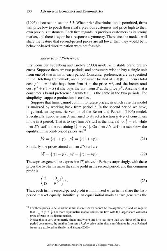
P1: FCW/
CUNY595-04 Cuny535/Blundell 0 521 87152 2 Printer: cupusbw August 16, 2006 17:35 Char Count= 0
130 Advances in Economics and Econometrics
(1996) discussed in section 3.3: When price discrimination is permitted, firmswill price low to poach their rival’s previous customers and price high to theirown previous customers. Each firm regards its previous customers as its strongmarket, and there is again best-response asymmetry. Therefore, the models willshare the feature that second-period prices are all lower than they would be ifbehavior-based discrimination were not feasible.
Stable Brand Preferences
First, consider Fudenberg and Tirole’s (2000) model with stable brand prefer-ences. Suppose there are two periods, and consumers wish to buy a single unitfrom one of two firms in each period. Consumer preferences are as specifiedin the Hotelling framework, and a consumer located at x ∈ [0, 1] incurs totalcost pA + t x if she buys from firm A at the price pA, and she incurs totalcost pB + t(1 − x) if she buys the unit from B at the price pB . Assume that aconsumer’s brand preference parameter x is the same in the two periods. Forsimplicity, suppose production is costless.
Suppose that firms cannot commit to future prices, in which case the modelis analyzed by working back from period 2. In the second period we have,in general, an asymmetric version of the Bester and Petrakis (1996) model.Specifically, suppose firm A managed to attract a fraction 1
2+ γ of consumers
in the first period. That is to say, firm A’s turf is the interval [0, 12
+ γ ], while
firm B’s turf is the remaining [ 12
+ γ , 1]. On firm A’s turf one can show theequilibrium second-period prices are70
pA2 = 2
3t(1 + γ ) ; pB
2 = 13t(1 + 4γ ) . (21)
Similarly, the prices aimed at firm B’s turf are
pB2 = 2
3t(1 − γ ) ; pA
2 = 13t(1 − 4γ ) . (22)
These prices generalize expression (7) above.71 Perhaps surprisingly, with theseprices the two firms make the same profit in the second period, and this commonprofit is (
5
18+ 10
9γ 2
)t . (23)
Thus, each firm’s second-period profit is minimized when firms share the first-period market equally. Intuitively, an equal initial market share generates the
70 For these prices to be valid the initial market shares cannot be too asymmetric, and we require
that − 14 ≤ γ ≤ 1
4 . For more asymmetric market shares, the firm with the larger share will set a
price of zero to its distant market.71 Notice that in very asymmetric situations, where one firm has more than two-thirds of the first-
period consumers, the smaller firm sets a higher price on its rival’s turf than on its own. Related
issues are explored in Shaffer and Zhang (2000).
Cambridge Collections Online © Cambridge University Press, 2006

P1: FCW/
CUNY595-04 Cuny535/Blundell 0 521 87152 2 Printer: cupusbw August 16, 2006 17:35 Char Count= 0
Recent Developments in the Economics of Price Discrimination 131
most informative outcome in the second period, and, in this setting with best-response asymmetry, more information destroys profit. When initial marketshares are very asymmetric, on the other hand, little is learned about mostconsumers’ brand preferences.72
Consider next the choice of first-period prices. Here, the outcome depends onthe sophistication of consumers. Suppose first that consumers are sophisticatedand anticipate the effect of initial market share on future prices in expressions(21)–(22). Notice that the larger “turf” faces higher second-period prices, whichimplies that, all else equal, a sophisticated consumer would prefer to purchasefrom the firm with fewer consumers in the first period. When both firms choosethe same initial price p1 say, they will share the market equally in the firstperiod (so γ = 0). Suppose instead that firm A slightly undercuts its rival inthe first period, and chooses price p1− ε. How many more consumers will itattract in the first period? Let us say that the marginal consumer in period 1is located at x = 1
2+ γ . When a consumer lies near the midpoint between the
two firms (γ small), she will surely switch firms in the second period in orderto take advantage of the poaching discount. Therefore, the marginal consumeris indifferent between buying from A-then-B or buying from B-then-A. Giventhe second-period prices in (21)–(22), γ satisfies
p1 − ε + (12
+ γ)t + δ
[13t(1 + 4γ ) + (
12
− γ)t]
= p1 + (12
− γ)t + δ
[13t(1 − 4γ ) + (
12
+ γ)t],
and so
γ = ε
2t(1 + 1
3δ) .
We deduce that sophisticated consumers react less sensitively to price reductionsin the first period than they would in a static model of this kind (when γ =ε/(2t)). The reason is that if a firm cuts its price in the first period, that brings adirect benefit to a consumer in the first period, but a disadvantage to the marginalconsumer at that firm in the second period, since her poaching price is raised.It follows that the first-period price is73
p1 = t(1 + 13δ) (24)
72 This is especially clear in the variant of the Fudenberg-Tirole model presented in chapter 3 of
Esteves (2004). Esteves assumes that consumer preferences follow a binary distribution, and
half the consumers prefer A by a fixed amount and half the consumers prefer B by the same fixed
amount. If firms set similar prices in the first period, they will share the market and consumer
tastes are fully revealed in the second period. If firms set significantly different first-period
prices then one firm attracts all consumers, and so nothing is learned in the second period and
subsequent profit is high.73 In fact, if a firm undercuts it rival in the first period this will affect its equilibrium profit in
the second period (which from (23) will rise). However, this effect is second-order for small
deviations, at least for this particular example, and so it plays no role in the calculation of the
equilibrium first-period price.
Cambridge Collections Online © Cambridge University Press, 2006

P1: FCW/
CUNY595-04 Cuny535/Blundell 0 521 87152 2 Printer: cupusbw August 16, 2006 17:35 Char Count= 0
132 Advances in Economics and Econometrics
while the second-period prices are as in (7) above:
p2 = 23t ; p2 = 1
3t. (25)
These second-period prices imply that the middle third of consumers switchfirms in the second period.
The sophisticated reasoning of the consumers in this model when there isbehavior-based discrimination might sometimes be implausible, especially innew markets where consumers have not yet grasped the firms’ pricing incen-tives. Suppose instead consumers are naive and do not foresee that when theybuy from the low price firm in the first period they will face higher prices inthe second period. Then, competition in the first period is just as in a standardstatic model, and the first-period price is p1 = t instead of the price in (24).Second-period prices are unaffected. Therefore, if consumers are naive thisimproves their position compared to when they are sophisticated. By contrast,in the monopoly situation of section 2.2, when consumers are naive they aretreated less favourably.
If the instrument of behavior-based price discrimination is not available, afirm’s price in each period is p1 = p2 = p2 = t . This implies that the first-period price is reduced (or unchanged with naive consumers) while second-period prices are raised compared to the situation with discrimination. Just aswith the Bester-Petrakis model, behavior-based price discrimination is sociallyinefficient, since in the second period a third of consumers buy from the less-preferred firm. When consumers are sophisticated, total discounted profit islower with discrimination.74 (When consumers are naive, firms are even worseoff with discrimination.) Therefore, when firms cannot commit to future prices,the ability to engage in behavior-based price discrimination reduces their profit.All consumers are at least weakly better off with discrimination.75 (And ifconsumers were naive, they would be even better off with discrimination.) Insum, a ban on this form of price discrimination makes consumers worse off,regardless of their presumed sophistication.76 (By contrast, in the monopolyanalysis of section 2.2, a ban on discrimination makes naive consumers betteroff.)
74 Industry profit with discrimination is (1 + 89 δ)t and without discrimination it is (1 + δ)t .
75 Without discrimination, a consumer pays a total discounted charge (1 + δ)t for the two
units. With discrimination, a consumer can buy a unit from the same firm in each pe-
riod, in which case expressions (24)–(25) imply that the total discounted charge is the same
(1 + δ)t . However, some consumers will be strictly better off by switching firms in the second
period.76 Villas-Boas (1999) presents related analysis when long-lived firms face overlapping generations
of short-lived consumers. One important difference with the Fudenberg-Tirole model is that a
firm only knows whether or not a consumer has previously purchased from it, and cannot
distinguish between its rival’s previous consumer and consumers who are new to the market.
He finds that, at least for patient firms and consumers, behavior-based discrimination causes all
prices to fall.
Cambridge Collections Online © Cambridge University Press, 2006

P1: FCW/
CUNY595-04 Cuny535/Blundell 0 521 87152 2 Printer: cupusbw August 16, 2006 17:35 Char Count= 0
Recent Developments in the Economics of Price Discrimination 133
Finally, a richer model would consider the impact of imperfect correlationof brand preference over time. If the first-period choice of firm was only animperfect signal of second-period brand preference, the temptation to set lowprices in the second period would be mitigated. In the extreme case where con-sumer brand preference was uncorrelated over time, a consumer’s initial choiceof firm would give no useful information about her subsequent preferences,and there would be no scope for behavior-based price discrimination. In gen-eral, we expect that when firms price discriminate, profit is decreasing in theextent of correlation of brand preference, while consumers benefit from highercorrelation.
Switching Costs
Second, consider Chen’s (1997b) model of switching costs. Again, there are twofirms each selling a product over two periods and consumers wish to purchase asingle unit in each of the two periods. If a consumer wishes to change supplierin the second period, she must incur a switching cost s. This cost varies acrossconsumers, and suppose s is uniformly distributed on the interval [0, t]. Thus,if firm A sets the second-period price pA
2 to its first-period customers, and iffirm B sets the poaching price pB
2 to the same group of customers, a customerwill switch to B whenever pA
2 > pB2 + s. If firms can price discriminate in the
second period, one can show the equilibrium prices are just as in the brandloyalty model in (25). (These are the prices regardless of market shares in thefirst period.) Just as in the Fudenberg-Tirole model, a third of consumers switchsuppliers in the second period, which is inefficient. If the number of firm A’sfirst-period customers is denoted n A (and the number of firm B’s customers isnB = 1 − n A), then firm A’s second-period profit is77
23n A p2 + 1
3nB p2 = 1
3t( 1
3+ n A) . (26)
Consider next the equilibrium first-period price. Since second-period pricesare the same for the two firms, a consumer will choose her initial supplierpurely on the basis of the lowest initial price. (The sophistication or otherwiseof consumers plays no role here.) Since each first-period consumer brings withher a second-period profit of 1
3t (see expression (26)), which is discounted
by δ, the equilibrium first-period price is p1 = − 13δt , which is below cost.
This feature is common in models of switching costs, where firms competehard to attract new consumers, anticipating consumers will generate high profitsubsequently. Therefore, we see a major difference between the two models ofFudenberg-Tirole and Chen: In the former, prices start high and then decrease,whereas here the reverse is seen.
77 Thus, in contrast to the Fudenberg-Tirole model, here the firm with the larger initial market
share makes a higher profit in the second period compared to its rival.
Cambridge Collections Online © Cambridge University Press, 2006

P1: FCW/
CUNY595-04 Cuny535/Blundell 0 521 87152 2 Printer: cupusbw August 16, 2006 17:35 Char Count= 0
134 Advances in Economics and Econometrics
By contrast, consider the situation where firms must charge a uniform pricein the second period. Unlike the case of price discrimination, the equilibriumsecond-period prices will here depend on initial market shares (as well as theassumed sophistication of consumers). If firms divide the market equally in thefirst period, the equilibrium price in the second period is p2 = t . If firms havedifferent market shares in the first period, the larger firm will choose the higherprice in the second period since it has a greater number of “captive” consumers.More precisely, the uniform prices in the second period given firm A’s initialmarket share n A ≥ 1
2are
pA = 1 + n A
3n At ; pB = 2 − n A
3n At ≤ pA . (27)
Both prices here are lower than when firms share the market equally (n A = 12),
and so second-period competition is intensified when firms have asymmetricinitial market shares. Second-period profits of the two firms are
π A2 = (1 + n A)2
9n At ; π B
2 = (2 − n A)2
9n At , (28)
and the firm with the larger market share obtains higher second-period profit.However, the profit of both firms is decreasing in the larger firm’s market shareand both firms are better off in the second period if they share the first-periodmarket equally.
From (27), in the first period sophisticated consumers may not react sen-sitively to price reductions since they know that if they buy from the largerfirm they will face a higher price in the second period. (Somewhat confusingly,this is the same mechanism as occurs in the Fudenberg-Tirole model with pricediscrimination.) A more important factor, which applies equally if consumersare naive, is that a firm has a strong incentive to set the same price as its rival inthe first period: From (28) a firm makes less second-period profit if it obtainsa higher or a lower market share in the first period, compared to when the twofirms share the initial market equally. As a result, there are multiple symmetricfirst-period prices that can be equilibria.78 Chen shows that firms are alwaysbetter off when behavior-based price discrimination is not possible, and it isambiguous whether consumers are better or worse off.79
78 Take for instance the situation where consumers are naive (which is not considered by Chen),
and in the first period consumers simply buy from the firm with the lower price (and the initial
market is equally divided if firms choose equal prices). If a firm undercuts its rival in the first
period it will attract all consumers and so make less profit in the second period (see (28)).
Similarly, if a firm sets a negative price in the first period, its rival may be unwilling to choose a
higher price because if it does so it will lose all its initial consumers and so make small profits
in the second period. One can show that any initial price in the range − 79 δt ≤ p1 ≤ 1
9 δt can be
an equilibrium in this context.79 See Taylor (2003) for an extension to Chen’s analysis in a number of important directions,
for instance to more than two periods and more than two firms. When there are more than
Cambridge Collections Online © Cambridge University Press, 2006

P1: FCW/
CUNY595-04 Cuny535/Blundell 0 521 87152 2 Printer: cupusbw August 16, 2006 17:35 Char Count= 0
Recent Developments in the Economics of Price Discrimination 135
5.2 Ex Ante Price Discrimination and Customer Loyalty
Finally, suppose firms can commit to all future prices.80 This setting, where firmscommit to explicit rewards for consumer loyalty, seems broadly applicable tofrequent flyer programes and the like. Consider the Fudenberg-Tirole setting ofrepeated sales to consumers with Hotelling preferences between the two firms’products. For simplicity, consider the extreme case in which a consumer’s brandpreferences are independently distributed over the two periods. Suppose furtherthat consumers know their second-period preferences at the time of their initialchoice of firm. In this situation, the mixed bundling model discussed in section4.2 applies immediately. Therefore, equilibrium prices are given in expression(18), which in the current notation become
p1 = p2 = 1112
t ; p2 = 512
t ,
and a repeat buyer receives a discount of 12t on her second unit. Here, compared
to the case where this form of ex ante dynamic pricing is not possible, firmssuffer from the profit-destroying impact of mixed bundling while consumersbenefit. Welfare is reduced since there is excessive customer loyalty.
Both kinds of price discrimination involve welfare losses, but of a differentform. Ex ante pricing involves excessive loyalty (one-stop shopping) while expost pricing induces excessive switching (two-stop shopping). The key differ-ence between the two models is that with ex post pricing the low price is aimedat the rival’s past customers, whereas with explicit ex ante loyalty schemes thelow price is aimed at a firm’s own past customers. This analysis suggests thatexplicit loyalty schemes have the potential to be pro-consumer, just like thecustomer poaching schemes of the previous section.81
two periods, the fact that a consumer switched supplier in the second period indicates that the
consumer has low switching costs, and this could generate more intense competition for him in
future periods.80 One issue is the realistic extent of commitment in this dynamic oligopoly context. For instance,
can firms commit to their second-period “poaching” price pi2? This seems less plausible than to
suppose firms can commit to their repeat price to loyal consumers, pi2. (One can say the same
for the monopoly analysis of section 2.2 – see footnote 18.) Section 5 of Fudenberg and Tirole
(2000) analyzes the use of long-term contracts where firms have the opportunity to poach their
rival’s customers in the second period at prices that are determined only in the second period.
Compared to when short-term contracts are employed, they show in the uniform example that
the use of long-term contracts reduces profit, reduces switching (which improves efficiency)
and boosts consumer surplus.81 For related analysis in the case where consumers do not know their future preferences at the
time of the initial choice, see Caminal and Matutes (1990), section 6 of Fudenberg and Tirole
(2000), and Caminal and Claici (2005). See Kim, Shi, and Srinivasan (2001) for an analysis of
reward programs as a price discrimination device to segment the high-volume and low-volume
markets. This paper also shows that firms might commit to use inefficient reward schemes (e.g.,
free gifts instead of price reductions), since that can sometimes act to soften subsequent price
competition.
Cambridge Collections Online © Cambridge University Press, 2006

P1: FCW/
CUNY595-04 Cuny535/Blundell 0 521 87152 2 Printer: cupusbw August 16, 2006 17:35 Char Count= 0
136 Advances in Economics and Econometrics
6 CONCLUDING COMMENTS
This paper has surveyed the recent literature on price discrimination, with afocus on the effects on industry outcomes when firms: (i) have access to moreinformation about their potential customers; (ii) can use more instruments whenchoosing their tariffs; and (iii) cannot commit to their pricing policy. The paperargued that the importance of each of these three factors has been increased dueto developments in marketing and e-commerce.
The analysis reported here is more suggestive than definitive, and was largelypresented through a series of worked examples. (Many of the papers from whichthis analysis was taken share this feature.) In particular, it is important to extendthe analysis beyond the examples presented here, which involved a relentlessuse of Hotelling demand specifications with unit demands and uniform distribu-tions. For instance, when consumers have inelastic demand there is no welfarebenefit when price discrimination causes prices to fall, and such a benefit wouldbe present in a richer model.82
Economic intuition seems to be better developed for the impact of moredetailed information than it is for the effects of more tariff instruments. Forinstance, the concept of best-response symmetry is a useful tool for predictingthe outcome of better information on profits and consumer surplus. However,there is as yet no such tool or intuition which can explain why competingfirms are (i) typically better off using two-part tariffs than linear prices (seesection 4.1) but (ii) typically worse off if they use bundling rather than separableprices (see section 4.2). There is plenty more work to be done in this excitingarea.
TECHNICAL APPENDIX
A PRIVATE INFORMATION
Here, the equilibrium prices in expression (8) are derived. Suppose that firm Bsets the price p when it sees the signal sR and the price p when it sees the signalsL . First consider the case when firm A sees the signal s A = sL for a consumer.What price should firm A offer this consumer? There are four relevant events:(i) the consumer is near to firm A and the rival firm also receives the signals B = sL and so sets the price p; (ii) the consumer is near to firm A but therival firm receives the ‘wrong’ signal s B = sR and so sets the high price p; (iii)the consumer is far from A and the rival firm also receives the signal s B = sL
and so sets the price p; and (iv) the consumer is far from A and the rival firmreceives the ‘correct’ signal s B = sR and so sets the price p. Conditional onfirm A seeing the signal s A = sL , the respective probabilities of the four eventsare α2, α(1 − α), (1 − α)2, α(1 − α). If firm A sets a price q to this consumer
82 See Armstrong and Vickers (2006) for some preliminary work on this extension.
Cambridge Collections Online © Cambridge University Press, 2006

P1: FCW/
CUNY595-04 Cuny535/Blundell 0 521 87152 2 Printer: cupusbw August 16, 2006 17:35 Char Count= 0
Recent Developments in the Economics of Price Discrimination 137
(which lies in the range p ≤ q ≤ p) then it will make the sale with probability
α2
(1 + p − q
t
)+ α(1 − α) + α(1 − α)
p − q
t.
(With case (ii) firm A will surely make the sale whenever it sets a price q ≤ p;with case (iii) it will surely not make the sale when q ≥ p.)
Suppose next that firm A observes signal s A = sR . In the same way, if it setsthe price q (which lies in the range p ≤ q ≤ p) its probability of making thesale is
α2 p − q
t+ α(1 − α)
(1 + p − q
t
)+ (1 − α)2 .
One can then show that symmetric equilibrium prices are given by expression(8).
B EFFECT OF MORE INSTRUMENTS
Here, the results reported in section 4.1 are derived. Let π A(u) and π B(u) be twoprofit-as-a-function-of-utility functions which satisfy (11). Firm i will choose ui
to maximize expression (10), and so equilibrium utilities {u A(t), u B(t)} satisfythe first-order conditions
π i (ui (t)) + (t + ui (t) − u j (t))π′i (ui (t)) = 0 , (29)
where ui (t) denotes the equilibrium utility offered by firm i when transport costis t . We wish to investigate the equilibrium in competitive markets, i.e., whent ≈ 0. Clearly, ui (0) = u. Differentiating (29) yields
π ′i u
′i + (1 + u′
i − u′j )π
′i + (t + ui − u j )π
′′i u′
i ≡ 0 .
Setting t = 0 here yields u′A(0) = u′
B(0) = −1. Differentiating (29) once more
yields
π ′′i (u′
i )2 + π ′
i u′′i + (u′′
i − u′′j )π
′i + 2(1 + u′
i − u′j )π
′′i u′
i
+ (t + ui − u j )(π′′′i (u′
i )2 + π ′′
i u′′i ) = 0 .
When t = 0 this simplifies to
u′′j (0) − 2u′′
i (0) = π ′′i (u) .
Solving this pair of simultaneous equations yields
u′′i (0) = −2π ′′
i (u) + π ′′j (u)
3,
which leads to expression (12).The equilibrium market share of firm i is approximately
ni = 1
2+ ui − u j
2t≈ 1
2+ 1
12(π ′′
j (u) − π ′′i (u))t .
Cambridge Collections Online © Cambridge University Press, 2006
P1: FCW/
CUNY595-04 Cuny535/Blundell 0 521 87152 2 Printer: cupusbw August 16, 2006 17:35 Char Count= 0
138 Advances in Economics and Econometrics
Aggregate consumer surplus in equilibrium is approximately equal to
U (t) ≈ u − 5t
4− t2
4(π ′′
A(u) + π ′′B(u)) . (30)
The per-consumer profit for firm i is
π i (ui (t)) ≈ t +(
5
6π ′′
i (u) + 1
6π ′′
j (u)
)t2 .
Therefore, the total profit of firm i (i.e., ni × π i ) is given by expression (13).Industry profit is therefore
�(t) ≈ t + t2
2(π ′′
A(u) + π ′′B(u)) .
Finally, from (30), total welfare (W = � + U ) is given by expression (14).
References
Acquisti, A., and H. Varian (2005): “Conditioning Prices on Purchase History,” Market-ing Science, 24(3), 367–381.
Anderson, S., and L. Leruth (1993): “Why Firms May Prefer Not to Price Discriminate
via Mixed Bundling,” International Journal of Industrial Organization, 11(1), 49–
61.Armstrong, M. (1999): “Price Discrimination by a Many-Product Firm,” Review of
Economic Studies, 66(1), 151–168.Armstrong, M., and J. Vickers (1993): “Price Discrimination, Competition and Regula-
tion,” Journal of Industrial Economics, 41(4), 335–360.——– (2001): “Competitive Price Discrimination,” Rand Journal of Economics, 32(4),
579–605.——– (2006): “Competitive Nonlinear Pricing and Bundling,” mimeo.Bakos, Y., and E. Brynjolfsson (1999): “Bundling Information Goods: Pricing, Profits,
and Efficiency,” Management Science, 45(12), 1613–1630.Baron, D., and D. Besanko (1984): “Regulation and Information in a Continuing Rela-
tionship,” Information Economics and Policy, 1(4), 267–302.Bernheim, D., and M. Whinston (1986): “Menu Auctions, Resource Allocation, and
Economic Influence,” Quarterly Journal of Economics, 101(1), 1–31.Bester, H., and E. Petrakis (1996): “Coupons and Oligopolistic Price Discrimination,”
International Journal of Industrial Organization, 14(2), 227–242.Bhaskar, V., and T. To (2004): “Is Perfect Price Discrimination Really Efficient? An
Analysis of Free Entry,” Rand Journal of Economics, 35(4), 762–776.Borenstein, S. (1985): “Price Discrimination in Free-Entry Markets,” Rand Journal of
Economics, 16(3), 380–397.Calzolari, G., and A. Pavan (2005): “On the Optimality of Privacy in Sequential Con-
tracting,” Journal of Economic Theory, forthcoming.Caminal, R., and A. Claici (2005): “Are Loyalty-Rewarding Pricing Schemes Anti-
Competitive?,” mimeo.Caminal, R., and C. Matutes (1990): “Endogenous Switching Costs in a Duopoly Model,”
International Journal of Industrial Organization, 8(3), 353–373.
Cambridge Collections Online © Cambridge University Press, 2006

P1: FCW/
CUNY595-04 Cuny535/Blundell 0 521 87152 2 Printer: cupusbw August 16, 2006 17:35 Char Count= 0
Recent Developments in the Economics of Price Discrimination 139
Carbajo, J., D. De Meza, and D. Seidman (1990): “A Strategic Motivation for Commodity
Bundling,” Journal of Industrial Economics, 38(3), 283–298.Chen, Y. (1997a): “Equilibrium Product Bundling,” Journal of Business, 70(1), 85–
103.——– (1997b): “Paying Customers to Switch,” Journal of Economics and Management
Strategy, 6(4), 877–897.——– (2006): “Marketing Innovation,” Journal of Economics and Management Strategy,
15(1), 101–123.Coase, R. (1972): “Durability and Monopoly,” Journal of Law and Economics, 15(1),
143–149.Cooper, T. (1986): “Most-Favored-Customer Pricing and Tacit Collusion,” Rand Journal
of Economics, 17(3), 377–388.Corts, K. (1998): “Third-Degree Price Discrimination in Oligopoly: All-Out Competi-
tion and Strategic Commitment,” Rand Journal of Economics, 29(2), 306–323.Cremer, J. (1984): “On the Economics of Repeat Buying,” Rand Journal of Economics,
15(3), 396–403.Dobson, P., and M. Waterson (2005): “Chain-Store Pricing Across Local Markets,”
Journal of Economics and Management Strategy, 14(1), 93–119.Economides, N. (1989): “The Desirability of Compatibility in the Absence of Network
Externalities,” American Economic Review, 71(5), 1165–1181.Ellison, G. (2005): “A Model of Add-on Pricing,” Quarterly Journal of Economics,
120(2), 585–637.——– (2006): “Bounded Rationality in Industrial Organization,” in Advances in Eco-
nomics and Economectrics: Theory and Applications: Ninth World Congress, ed. by
R. Blundell, W. Newey, and T. Persson. Cambridge University Press, Cambridge,
UK.Esteves, R. B. (2004): “Competitive Behaviour-Based Price Discrimination,” PhD thesis,
Oxford University.Fudenberg, D., and J. Tirole (2000): “Customer Poaching and Brand Switching,” Rand
Journal of Economics, 31(4), 634–657.Fudenberg, D., and M. Villas-Boas (2005): “Behaviour-Based Price Discrimination and
Customer Recognition,” in Handbook on Economics and Information Systems, ed. by
T. Hendershott. North-Holland, Amsterdam, forthcoming.Gans, J., and S. King (2006): “Paying for Loyalty: Product Bundling in Oligopoly,”
Journal of Industrial Economics, 54(1), 43–62.Geng, X., M. Stinchcombe, and A. Whinston (2005): “Bundling Information Goods of
Decreasing Value,” Management Science, 51(4), 662–667.Hart, O., and J. Tirole (1988): “Contract Renegotiation and Coasian Dynamics,” Review
of Economic Studies, 55(4), 509–540.Kim, B.-D., M. Shi, and K. Srinivasan (2001): “Reward Programs and Tacit Collusion,”
Marketing Science, 20(2), 99–120.Klemperer, P. (1988): “The Competitiveness of Markets with Switching Costs,” Rand
Journal of Economics, 18(1), 138–150.——– (1992): “Equilibrium Product Lines: Competing Head-to-Head May be Less
Competitive,” American Economic Review, 82(4), 740–755.Laffont, J.-J., and D. Martimort (2002): The Theory of Incentives: The Principal-Agent
Model. Princeton University Press, Princeton, NJ.Liu, Q., and K. Serfes (2004): “Quality of Information and Oligopolistic Price Discrim-
ination,” Journal of Economics and Management Strategy, 13(4), 671–702.Matutes, C., and P. Regibeau (1988): “Mix and Match: Product Compatibility without
Network Externalities,” Rand Journal of Economics, 19(2), 221–234.
Cambridge Collections Online © Cambridge University Press, 2006

P1: FCW/
CUNY595-04 Cuny535/Blundell 0 521 87152 2 Printer: cupusbw August 16, 2006 17:35 Char Count= 0
140 Advances in Economics and Econometrics
——– (1992): “Compatibility and Bundling of Complementary Goods in a Duopoly,”
Journal of Industrial Economics, 40(1), 37–54.Miravete, E., and L.-H. Roller (2004): “Competitive Nonlinear Pricing in Duopoly
Equilibrium: The Early U.S. Cellular Telephone industry,” mimeo.Nahata, B., K. Ostaszewski, and P. Sahoo (1990): “Direction of Price Changes in
Third-Degree Price Discrimination,” American Economic Review, 80(5), 1254–
1258.Nalebuff, B. (2000): “Competing Against Bundles,” in Incentives, Organization,
and Public Economics, ed. by G. Myles and P. Hammond. Oxford University
Press.——– (2004): “Bundling as an Entry Barrier,” Quarterly Journal of Economics, 119(1),
159–188.Nevo, A., and C. Wolfram (2002): “Why do Manufacturers Issue Coupons? An Empirical
Analysis of Breakfast Cereals,” Rand Journal of Economics, 33(2), 319–339.Odlyzko, A. (2003): “Privacy, Economics, and Price Discrimination on the Inter-
net,” ICEC2003: Fifth International Conference on Electronic Commerce, pp. 355–
366.Rey, P., and J. Tirole (2006): “A Primer on Foreclosure,” in Handbook of Industrial Orga-
nization: Volume III, ed. by M. Armstrong and R. Porter. North-Holland, Amsterdam,
forthcoming.Rochet, J.-C., and L. Stole (2002): “Nonlinear Pricing with Random Participation,”
Review of Economic Studies, 69(1), 277–311.Rothschild, M. (1974): “A Two-Armed Bandit Theory of Market Pricing,” Journal of
Economic Theory, 9, 185–202.Shaffer, G., and J. Zhang (1995): “Competitive Coupon Targeting,” Marketing Science,
14(4), 395–415.——– (2000): “Pay to Switch or Pay to Stay: Preference-Based Price Discrimination
in Markets with Switching Costs,” Journal of Economics and Management Strategy,9(3), 397–424.
Spulber, D. (1979): “Noncooperative Equilibrium with Price Discriminating Firms,”
Economics Letters, 4, 221–227.——– (1989): “Product Variety and Competitive Discounts,” Journal of Economic The-
ory, 48(2), 510–525.Stigler, G. (1987): Theory of Price. Macmillan, New York.Stole, L. (1995): “Nonlinear Pricing and Oligopoly,” Journal of Economics and Man-
agement Strategy, 4(4), 529–562.——– (2006): “Price Discrimination and Imperfect Competition,” in Handbook of In
dustrial Organization: Volume III, ed. by M. Armstrong, and R. Porter. North-Holland,
Amsterdam, forthcoming.Taylor, C. (2003): “Supplier Surfing: Competition and Consumer Behavior in Subscrip-
tion Markets,” Rand Journal of Economics, 34(2), 223–246.——– (2004): “Consumer Privacy and the Market for Customer Information,” Rand
Journal of Economics, 35(4), 631–650.Thanassoulis, J. (2006): “Competitive Bundling and Mixed Consumer Surplus,” mimeo.Thisse, J.-F., and X. Vives (1988): “On the Strategic Choice of Spatial Price Policy,”
American Economic Review, 78(1), 122–137.Varian, H. (1980): “A Model of Sales,” American Economic Review, 70(4), 651–659.Vickers, J. (2005): “Abuse of Market Power,” Economic Journal, 115(504), F244–
F261.Villas-Boas, J. M. (1999): “Dynamic Competition with Customer Recognition,” Rand
Journal of Economics, 30(4), 604–631.
Cambridge Collections Online © Cambridge University Press, 2006

P1: FCW/
CUNY595-04 Cuny535/Blundell 0 521 87152 2 Printer: cupusbw August 16, 2006 17:35 Char Count= 0
Recent Developments in the Economics of Price Discrimination 141
——– (2004): “Price Cycles in Markets with Customer Recognition,” Rand Journal ofEconomics, 35(3), 486–501.
Wallace, R. (2004): “Preference-Based Discrimination and Profit: On the Profitability
of Discriminatory Spatial Policy,” Journal of Economics and Management Strategy,13(2), 351–369.
Whinston, M. (1990): “Tying, Foreclosure and Exclusion,” American Economic Review,80(4), 837–859.
Yin, X. (2004): “Two-Part Tariff Competition in Duopoly,” International Journal ofIndustrial Organization, 22(6), 799–820.
Cambridge Collections Online © Cambridge University Press, 2006