1

Recent global-warming hiatus tied to equatorial Pacific surface cooling

Yu Kosaka1 and Shang-Ping Xie

1,2,3

1Scripps Institution of Oceanography, University of California, San Diego, 9500

Gilman Drive MC 0230, La Jolla, California 92093, USA

2Physical Oceanography Laboratory and Ocean–Atmosphere Interaction and Climate

Laboratory, Ocean University of China, 238 Songling Road, Qingdao, 266100, China

3International Pacific Research Center, SOEST, University of Hawaii at Manoa, 1680

East West Road, Honolulu, Hawaii 96822, USA

Despite the continued increase of atmospheric greenhouse gases, the

annual-mean global temperature has not risen in this century1,2, challenging the

prevailing view that anthropogenic forcing causes climate warming. Various

mechanisms have been proposed for this hiatus of global warming3-6, but their

relative importance has not been quantified, hampering observational estimates of

climate sensitivity. Here we show that accounting for recent cooling in the eastern

equatorial Pacific reconciles climate simulations and observations. We present a

novel method to unravel mechanisms for global temperature change by

prescribing the observed history of sea surface temperature over the deep tropical

Pacific in a climate model, in addition to radiative forcing. Although the surface

temperature prescription is limited to only 8.2% of the global surface, our model

reproduces the annual-mean global temperature remarkably well with r = 0.97 for

1970-2012 (a period including the current hiatus and an accelerated global

warming). Moreover, our simulation captures major seasonal and regional

characteristics of the hiatus, including the intensified Walker circulation, the

2

winter cooling in northwestern and prolonged drought in southern North America.

Our results show that the current hiatus is part of natural climate variability, tied

specifically to a La Niña-like decadal cooling. While similar decadal hiatus events

may occur in the future, multi-decadal warming trend is very likely to continue

with greenhouse gas increase.

Daily mean carbon dioxide at Mauna Loa of Hawaii exceeded 400ppm for the

first time in May 2013. Whereas the greenhouse gas increase has been shown to cause

the centennial trend of global temperature rise since the industrial revolution7, global

temperature has remained flat for the past 15 years (Extended Data Fig. 1). Two schools

of idea exist regarding what causes this hiatus of global warming: one suggests a

slowdown in radiative forcing due to the stratospheric water vapour3, the rapid increase

of stratospheric and tropospheric aerosols4,5

, and the solar minimum around 2009 (ref.

5), while the other considers the hiatus as part of natural variability, especially a La

Niña-like cooling in the tropical Pacific6. A quantitative method is necessary to evaluate

the relative importance of these mechanisms. Adding to the confusion that, amid the

global warming hiatus, record heat waves hit Russia (2010 summer) and US (July 2012),

and Arctic sea ice reached record lows (Extended Data Fig. 1). Attributing these

regional climate changes requires a dynamic approach. Here we use an advanced

climate model that takes radiative forcing and tropical Pacific sea surface temperature

(SST) as input. The simulated global-mean temperature is in excellent agreement with

observations, showing that the decadal cooling of the tropical Pacific causes the current

hiatus. Our dynamic-model based attribution has a distinct advantage over the empirical

approach2,5

by revealing seasonal and regional aspects of the hiatus.

Three sets of experiments were performed based on the Geophysical Fluid

Dynamics Laboratory (GFDL) coupled model version 2.1 (CM2.1) (ref. 8). The

historical (HIST) experiment is forced with observed atmospheric composition changes

3

and the solar cycle. In Pacific Ocean-Global Atmosphere (POGA) experiments, SST

anomalies in the equatorial eastern Pacific (8.2% of the Earth surface) follow the

observed evolution (see Methods). In POGA-H, the radiative forcing is identical to

HIST, while in the POGA control experiment (POGA-C) it is fixed at 1990 value.

Outside the equatorial eastern Pacific, the atmosphere and ocean are fully coupled and

free to evolve.

Figure 1 compares the observed and simulated global near-surface temperature. In

HIST, the annual-mean temperature keeps rising in response to the increased radiative

forcing, with expanding departures from observations for the recent decade (Fig. 1a).

POGA-H well reproduces the observed record (Extended Data Table 1). For a 43-year

period after 1970 when equatorial Pacific SST data are more reliable, correlation (r)

with observations is r = 0.97 for POGA-H, due largely to the long-term trend (r = 0.90

for HIST). Detrended, POGA-H still reproduces the observations at r = 0.70, whereas it

falls to 0.26 in HIST. POGA-C illustrates the tropical control of the global temperature

with constant radiative forcing, with the global-mean temperature closely following

tropical Pacific variability (Fig. 1b). The global-mean surface air temperature (SAT)

changes by 0.29ºC in response to a 1ºC SAT anomaly over the equatorial eastern Pacific.

For the recent decade, the decrease in tropical Pacific SST has lowered the global

temperature by ~0.15ºC compared to the 1990s (Fig. 1b), opposing the radiative forcing

effect and causing the hiatus. Likewise an El Niño-like trend in the tropics9 accelerated

the global warming from the 1970s to late 1990s10

(Extended Data Table 1).

The POGA experimental design has been used to study global teleconnections of

interannual El Niño-Southern Oscillation (ENSO)11,12

. Here we have presented a novel

application of POGA and demonstrated its skill in simulating the observed decadal

modulations of the global warming trend including the peculiar hiatus. Our results show

that the two-parameter (radiative forcing and tropical Pacific SST) system is remarkably

4

skilful in reproducing the observed global-mean temperature record, superior over the

HIST results with radiative forcing alone. In individual HIST realizations, hiatus events

feature decadal La Niña-like cooling in the tropical Pacific6 (Extended Data Fig. 2), but

POGA-H enables a direct year-by-year comparison with the observed timeseries of

global temperature, not just the statistics from unconstrained coupled runs.

We focus on trends over the recent 11 years from 2002 to 2012, to avoid the

strong 1997/98 El Niño event and the following 3-year La Niña events. Net downward

radiation and ocean heat content in POGA-H have continued to increase during the

global SAT hiatus6 (Extended Data Fig. 3). The SAT hiatus is confined to the cold

season13

(referred to the boreal seasons hereafter), with a decadal cooling trend for

November-April, while the global temperature continues to rise during summer (Fig.

1c). POGA-H reproduces this seasonal cycle of the hiatus, albeit with a somewhat

reduced amplitude. Although the La Niña-like cooling trend in the tropical Pacific is

similar between winter and summer (Extended Data Fig. 4a), stationary/transient eddies,

the dominant mechanism for meridional heat transport14

, are stronger in winter than

summer. As a result, the tropical cooling effect on the extratropics is most pronounced

in winter (seasonality of the temperature trend in the Southern Hemisphere extratropics

is weak). The tropical influence on the Northern Hemisphere (NH) extratropics is weak

during the summer, allowing the radiative forcing to continue the warming trend during

the recent decade (Extended Data Fig. 4b).

This seasonal contrast is evident also in HIST. For 1970-2040, a period when the

ensemble-mean global temperature shows a steady increase in HIST, the probability

density function (PDF) for 11-year trend is similar between winter and summer for

tropical temperature, with means both around 0.25ºC (Extended Data Fig. 4c). The PDF

is much broader for winter than summer for NH extratropical temperature (Extended

Data Fig. 4d). The chance for 11-year temperature change to fall below –0.3ºC is 8% for

5

winter but only 0.7% for summer in the NH extratropics (~4% in the tropics for both

seasons). The 11-fold increase in the chance of an extratropical cooling in winter is due

partly to the stronger tropical influence than in summer.

We examine regional climate change associated with the hiatus. While models

project a slowdown of the Walker circulation in global warming15

, the Pacific Walker

cell intensified during the past decade (Fig. 2c). POGA-H captures this circulation

change, forced by the SST cooling across the tropical Pacific (Fig. 2d). As in

interannual ENSO, the tropical Pacific cooling excites global teleconnections in

December-January-February (DJF; the season is denoted with first letters of the months).

SST changes in POGA-H are in broad agreement with observations over the Indian

Ocean, South Atlantic, and Pacific outside the restoring domain (Figs. 2a,b). The model

reproduces the weakening of the Aleutian low as the response of the Pacific-North

American pattern to tropical Pacific cooling11

(Figs. 2c,d). As a result, the SAT change

over North America is well reproduced, including a pronounced cooling in the

northwestern continent. The model fails to simulate the SAT and sea-level pressure

(SLP) changes over Eurasia, suggesting that they are due to internal variability

unrelated to tropical forcing (Extended Data Fig. 5, left panels).

In summer, the broad agreement between simulated and observed SST remains

over the Pacific (Figs. 3a,b) but the tropical influence on SAT over extratropical Eurasia

and Arctic is weak (Extended Data Fig. 5, right panels), and the increasing radiative

forcing permits heat waves to develop in NH continents and Arctic sea ice to melt. (The

model does not produce the record shrinkage of Arctic sea ice because of model biases

and natural variability in the Arctic.) We note that the observed JJA warming in western

midlatitude Eurasia is much more intense than in POGA-H as heat waves there (2003 in

central Europe and 2010 in Russia) are associated with long-lasting blocking events

unrelated to tropical variability16

. POGA-H captures the rainfall decrease and warming

6

over the southern US, changes associated with prolonged droughts of record severity in

Texas17

. The southern US anomalies are probably tropical-forced (Extended Data Fig. 5,

right panels), for which winter-spring precipitation deficits and land-surface memory

processes are likely important17

. Likewise, during the epoch of accelerated global

warming from the 1970s to late 1990s, the southern US appears as a warming hole18

, a

spatial pattern likely tied to tropical SST (Extended Data Fig. 6).

We have presented a unique dynamic-based method for quantitative attributions of

decadal modulations of global warming. By prescribing observed SST in only 8.2% of

the Earth’s surface, POGA-H reproduces the observed timeseries of global-mean

temperature strikingly well, including interannual to decadal variability. The

comparison between HIST and POGA-H indicates that the decadal cooling of the

tropical Pacific is the culprit of the current hiatus. In addition, POGA-H reproduces the

seasonal and key regional patterns of the hiatus. The La Niña-like cooling in the tropics

affects the extratropics strongly in boreal winter, causing a global cooling, weakened

Aleutian low, and enhanced cooling over northwestern North America among other

regional anomalies. In boreal summer, by contrast, the NH extratropics is largely

shielded from the tropical influence, and the temperature continues to rise in response to

the increased radiative forcing.

A question remains whether the La Niña-like decadal trend is internal or forced.

We note the following facts: i) The tropical Pacific features pronounced low-frequency

SST variability (Extended Data Fig. 7), so large that the pattern of modest forced

response has yet emerged from observations (Fig. 1b). ii) All the climate models project

a tropical Pacific warming in response to increased greenhouse gas concentrations7. We

conclude that the recent cooling of the tropical Pacific and hence the current hiatus are

likely due to natural internal variability rather than a forced response. As such, the

hiatus is temporary, and global warming will return when the tropical Pacific swings

7

back to a warm state. Similar hiatus events may occur in the future and are difficult to

predict at multi-year leads due to limited predictability of tropical Pacific SST. We

showed that when taking place, such events are accompanied by characteristic regional

patterns including an intensified Walker circulation, weakened Aleutian low and

prolonged droughts in the southern US.

While radiative-forced response will become increasingly important, deviations

from the forced response are substantial at any given time, especially on regional

scales19

. Quantitative tools like our POGA-H are crucial to attribute the causes of

regional climate anomalies17

. The current hiatus illustrates the global influence of

tropical Pacific SST, and a dependency of climate sensitivity on the spatial pattern of

tropical ocean warming, which itself is uncertain in observations20

and among

models21,22

. This highlights the need to develop predictive pattern dynamics constrained

by observations.

8

Methods summary

We use the Hadley Centre-Climate Research Unit combined land SAT and SST

(HadCRUT) version 4.1.1.0 (ref. 23), the Hadley Centre mean SLP dataset version 2

(HadSLP2, ref. 24) and monthly precipitation data from Global Precipitation

Climatology Project (GPCP) version 2.2 (ref. 25). We examine three sets of coupled

model experiments based on GFDL CM2.1 (ref. 8). HIST is forced by historical

radiative forcing for 1861-2005 and Representative Concentration Pathway 4.5

(RCP4.5) for 2006-2040, based on Coupled Model Intercomparison Project phase 5

(CMIP5, ref. 26). In POGA-H and POGA-C experiments, SST is restored to the model

climatology plus historical anomaly by a Newtonian cooling over the deep tropical

eastern Pacific. The restoring timescale is 10 days for a 50 m mixed layer. Figures 2b

and 3b shows the region where SST is restored; within the inner box the ocean surface

heat flux is fully overridden, while in the buffer zone between the inner and outer boxes,

the flux is blended with the model-diagnosed one. In POGA-H, radiative forcing is

identical to HIST, while it is fixed at 1990 values in POGA-C. The three experiments

consist of 10 member runs each.

9

References

1. Easterling, D. R. & Wehner, M. F. Is the climate warming or cooling? Geophys.

Res. Lett. 36, L08706 (2009).

2. Foster, G. & Rahmstorf, S. Global temperature evolution 1979-2010. Environ.

Res. Lett. 6, 044022, doi:10.1088/1748-9326/6/4/044022 (2011).

3. Solomon, S. et al. Contributions of stratospheric water vapor to decadal changes

in the rate of global warming. Science 327, 1219–1223 (2010).

4. Solomon, S. et al. The persistently variable "background" stratospheric aerosol

layer and global climate change. Science 333, 866–870 (2011).

5. Kaufmann, R. K., Kauppi, H., Mann, M. L. & Stock, J. H. Reconciling

anthropogenic climate change with observed temperature 1998-2008. Proc. Natl.

Acad. Sci. USA 108, 11790–11793 (2011).

6. Meehl, G. A., Arblaster, J. M., Fasullo, J. T., Hu, A. & Trenberth, K. E.

Model-based evidence of deep-ocean heat uptake during surface-temperature

hiatus periods. Nature Clim. Change 1, 360–364 (2011).

7. Meehl, G. A. et al. in Climate Change 2007: The Physical Science Basis (eds.

Solomon, S. et al.). 747–845 (Cambridge University Press, 2007).

8. Delworth, T. L. et al. GFDL's CM2 global coupled climate models. Part I:

Formulation and simulation characteristics. J. Clim. 19, 643–674 (2006).

9. Zhang, Y., Wallace, J. M. & Battisti, D. S. ENSO-like interdecadal variability:

1900–93. J. Clim. 10, 1004–1020 (1997).

10. Meehl, G. A., Hu, A., Arblaster, J., Fasullo, J. & Trenberth, K. E. Externally

forced and internally generated decadal climate variability associated with the

Interdecadal Pacific Oscillation. J. Clim., doi: 10.1175/JCLI-D-12-00548.1 (in

press).

11. Alexander, M. A. et al. The atmospheric bridge: The influence of ENSO

teleconnections on air-sea interaction over the global oceans. J. Clim. 15,

2205–2231 (2002).

12. Lau, N.-C. & Nath, M. J. The role of the ''atmospheric bridge'' in linking tropical

Pacific ENSO events to extratropical SST anomalies. J. Clim. 9, 2036–2057

(1996).

10

13. Cohen, J. L., Furtado, J. C., Barlow, M., Alexeev, V. A. & Cherry, J. E.

Asymmetric seasonal temperature trends. Geophys. Res. Lett. 39, L04705

(2012).

14. Trenberth, K. E., Caron, J. M., Stepaniak, D. P. & Worley, S. Evolution of El

Niño-Southern Oscillation and global atmospheric surface temperatures. J.

Geophys. Res. 107, AAC 5-1–AAC 5-17 (2002).

15. Vecchi, G. A. et al. Weakening of tropical Pacific atmospheric circulation due to

anthropogenic forcing. Nature 441, 73–76 (2006).

16. Barriopedro, D., Garcia-Herrera, R., Lupo, A. R. & Hernandez, E. A

climatology of northern hemisphere blocking. J. Clim. 19, 1042–1063 (2006).

17. Hoerling, M. et al. Anatomy of an extreme event. J. Clim. 26, 2811–2832

(2013).

18. Wang, H. et al. Attribution of the seasonality and regionality in climate trends

over the United States during 1950-2000. J. Clim. 22, 2571–2590 (2009).

19. Deser, C., Knutti, R., Solomon, S. & Phillips, A. S. Communication of the role

of natural variability in future North American climate. Nature Clim. Change 2,

775–779 (2012).

20. Tokinaga, H., Xie, S.-P., Deser, C., Kosaka, Y. & Okumura, Y. M. Slowdown of

the Walker circulation driven by tropical Indo-Pacific warming. Nature 491,

439–443 (2012).

21. DiNezio, P. N., Clement, A. C., Vecchi, G. A., Soden, B. J. & Kirtman, B. P.

Climate response of the equatorial Pacific to global qarming. J. Clim. 22,

4873–4892 (2009).

22. Ma, J. & Xie, S.-P. Regional patterns of sea surface temperature change: A

source of uncertainty in future projections of precipitation and atmospheric

circulation. J. Clim. 26, 2482–2501 (2013).

23. Morice, C. P., Kennedy, J. J., Rayner, N. A. & Jones, P. D. Quantifying

uncertainties in global and regional temperature change using an ensemble of

observational estimates: The HadCRUT4 data set. J. Geophys. Res. 117,

D08101 (2012).

24. Allan, R. & Ansell, T. A new globally complete monthly historical gridded

mean sea level pressure dataset (HadSLP2): 1850-2004. J. Clim. 19, 5816–5842

(2006).

11

25. Adler, R. F. et al. The version-2 global precipitation climatology project (GPCP)

monthly precipitation analysis (1979-present). J. Hydrometeorol. 4, 1147–1167

(2003).

26. Taylor, K. E., Stouffer, R. J. & Meehl, G. A. An overview of CMIP5 and the

experiment design. Bull. Am. Meteorol. Soc. 93, 485–498 (2012).

Acknowledgements. We wish to thank GFDL model developers for making CM2.1 available; L. Xu, Y.

Du, N. C. Johnson and C. Deser for discussions. The work was supported by NSF (ATM-0854365), the

National Basic Research Program of China (2012CB955600), and NOAA (NA10OAR4310250).

Author Contributions. Y.K. and S.-P.X. designed the model experiments. Y.K. performed the

experiments and analysis. S.-P.X. and Y.K. wrote the manuscript.

Author Information. The authors declare no competing financial interests. Correspondence and requests

for materials should be addressed to S.-P.X. (sxie@ucsd.edu).

12

Figure legends

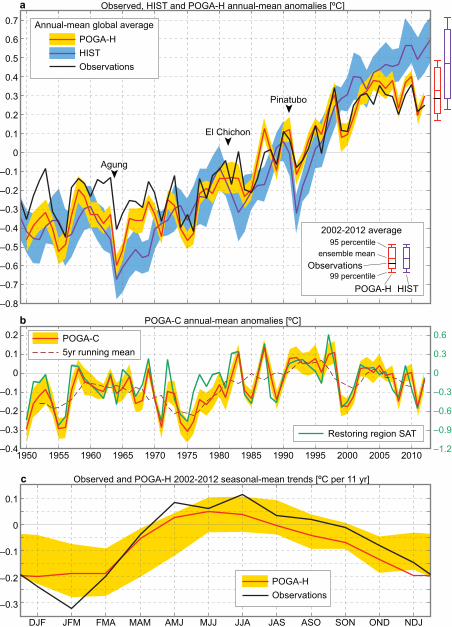
Figure 1. Observed and simulated global temperature trends. Annual-mean

timeseries based on a, observations, HIST and POGA-H; and b, POGA-C. Anomalies

are deviations from the 1980-1999 averages, except for HIST, for which the reference is

the 1980-1999 average of POGA-H. SAT anomalies over the restoring region are

plotted in b, with the axis on the right. Major volcanic eruptions are indicated in a. c,

Trends of seasonal global temperature for 2002-2012 in observations and POGA-H.

Shading represents 95% confidence interval of ensemble means. Bars on the right of a

show ranges of ensemble spreads of the 2002-2012 averages.

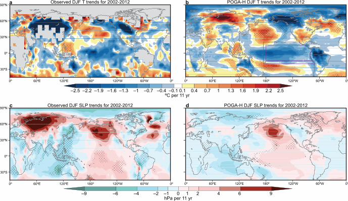
Figure 2. Observed and simulated trend patterns in boreal winter for 2002-2012.

a-b, Near-surface temperature, and c-d, SLP, from observations (left panels) and

POGA-H (right panels) in DJF. Grey shading represent missing values. Stippling

indicate regions exceeding 95% statistical confidence. Purple boxes in b show the

restoring region of POGA experiments.

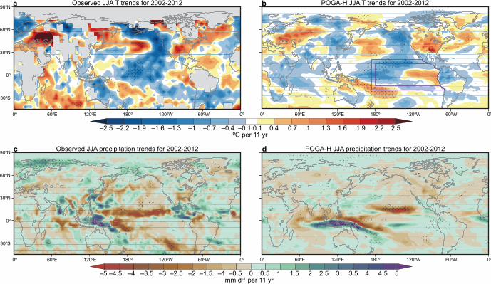
Figure 3. Observed and simulated trend patterns in boreal summer for 2002-2012.

Same as Fig. 2, but a-b, near-surface temperature and c-d, precipitation in JJA.

13

Methods

Gridded observational datasets. We use the Hadley Centre-Climate Research Unit

combined land SAT and SST (HadCRUT) version 4.1.1.0

(http://www.metoffice.gov.uk/hadobs/crutem4/; ref. 23); the Hadley Centre mean SLP

dataset version 2 (HadSLP2, http://www.metoffice.gov.uk/hadobs/hadslp2/; ref. 24);

monthly precipitation data from Global Precipitation Climatology Project (GPCP)

version 2.2 (http://www.gewex.org/gpcp.html; ref. 25). HadCRUT is compared with

SAT of the model.

Model experiments. We use GFDL CM2.1 (ref. 8). HIST, POGA-H and POGA-C

experiments are made of 10 member runs each. HIST is forced by historical radiative

forcing of the Coupled Model Intercomparison Project phase 5 (CMIP5, ref. 26) for

1861-2005 and extends to 2040 with Representative Concentration Pathway 4.5

(RCP4.5). The forcing includes greenhouse gases, aerosols, ozone, the solar activity

cycle (repeating the cycle for 1996-2008 after 2009) and land use.

In POGA experiments, deep tropical eastern Pacific SST is restored to the model

climatology plus historical anomaly, by overriding surface sensible heat flux to ocean

( F↓) with

F↓ = 1−α( ) F

*

↓ +α cD τ( ) ⋅ ′T −T*′( ) .

Here the prime indicates the anomaly, asterisks represent model-diagnosed values, and

T denotes SST. The reference temperature anomaly T' is based on Hadley Centre Ice

and SST version 1 (HadISST1, http://www.metoffice.gov.uk/hadobs/hadisst/; ref. 27).

The model anomaly is the deviation from the climatology of a 300-year control

experiment. c is the specific heat of sea water, D = 50 m the typical depth of the

ocean-mixed layer, and IJ = 10 d is the restoring timescale. Figures 2b and 3b show the

14

region where SST is restored: Į = 1 within the inner box, linearly reduced to zero in the

buffer zone from the inner to the outer boxes. In POGA-H, radiative forcing is identical

to HIST, while it is fixed at 1990 values in POGA-C.

Trend estimates. Trends are calculated as the Sen median slope28

. For observed surface

temperature, trends are calculated for grid boxes where data are available for > 80% of

years with at least one month per season. Mann-Kendall test is performed for statistical

significance of trends shown in Figs. 2, 3 and Extended Data Fig. 6, while t-test is

applied for significance of composited differences/anomalies of trends (Extended Data

Table 1 and Extended Data Fig. 2). In Extended Data Figs. 4c,d, the trends are evaluated

every 4 years for individual members of HIST, and PDFs are plotted with a kernel

density estimation and a Gaussian smoother.

Decadal variability. In Extended Data Figs. 5 and 7, Lanczos low-pass filter with a

half-power frequency of 8 years has been applied to extract decadal variability.

Extended Data Fig. 5 shows decadal anomalies obtained from a regression analysis,

with their statistical significance tested with t-statistic.

Other observational datasets. For Extended Data Fig. 1, we also use the Southern

Oscillation Index (http://www.cpc.ncep.noaa.gov/data/indices/; ref. 29) and US National

Snow and Ice Data Center Arctic sea ice extent (http://nsidc.org/data/seaice_index/; ref.

30).

27. Rayner, N. A. et al. Global analyses of sea surface temperature, sea ice, and

night marine air temperature since the late nineteenth century. J. Geophys. Res.

108, 4407 (2003).

28. Sen, P. K. Estimates of regression coefficient based on Kendall's tau. J. Am.

Stat. Assoc. 63, 1379–1389 (1968).

15

29. Trenberth, K. E. Signal versus noise in the Southern Oscillation. Mon. Wea. Rev.

112, 326–332 (1984).

30. Fetterer, F. & Knowles, K. Sea ice index monitors polar ice extent. Eos 85, 163

(2004).

16

Title and Legend for Extended Data Table

Extended Data Table 1. Evaluation of simulations of observed global mean

temperature and its trend

All based on ensemble-mean values. Correlations and root mean square errors are

evaluated for 1970-2012 with respect to observations. The trends are significantly

different between the experiments at P < 0.01 (2002-2012) and P < 0.05 (1971-1997)

based on t-test applied for the ensembles.

Legends for Extended Data figures

Extended Data Figure 1. Observed climate indices for the recent decade. (From top

to bottom) Annual-mean global near-surface temperature anomalies from the 1980-1999

average, DJF Southern Oscillation Index, DJF SLP near Aleutian Islands (40º-60ºN,

170º-120{W), JJA SAT over the US (30º-45ºN, 110º-80ºW), and September Arctic sea

ice extent.

Extended Data Figure 2. 11-year trends of annual-mean SAT composited for 34

hiatus events in HIST. The hiatus events are chosen for which annual-mean global

SAT trends are smaller than their ensemble mean minus 0.3 ºC per 11 yr. Stippling

indicates 95% statistical confidence. Note that a typical hiatus in HIST features a La

Niña-like pattern in the tropics and SST cooling around the Aleutian Islands, patterns

similar to the current hiatus event.

Extended Data Figure 3. Net radiative imbalance and ocean heat content increase

in POGA-H and HIST. a-b, Net radiative imbalance at the top-of-atmosphere. Positive

values indicate net energy flux into the planet. c-d, Ocean heat content deviations from

17

1950 values for each ensemble member. POGA-H (left panels) and HIST (right panels).

Shading represents 95% confidence interval of ensemble means. Major volcanic

eruptions are indicated. The radiative imbalance has remained positive and ocean heat

content has kept increasing for the recent decade in both of the experiments. Note that

the energy budget is not closed in POGA.

Extended Data Figure 4. Seasonal dependency of regional temperature trends. a-b

Observed temperature anomalies (solid) and their trends (dashed) for the recent decade

(ºC). c-d PDFs (curves) and means (vertical lines) of 11-year SAT trends in HIST for

1971-2040. Temperature has been averaged over the tropics (20ºS-20ºN; left panels)

and the northern extratropics (20º-90ºN; right panels) for JJA (red) and DJF (blue). Note

that the northern extratropics features a larger PDF spread in winter than summer, in

contrast to a high similarity in the tropics. The winter spread is also greater in the

extratropics than the tropics, whereas the opposite is true for summer.

Extended Data Figure 5. Decadal anomalies associated with SST cooling over the

equatorial Pacific. Low-pass filtered inter-member anomalies in HIST regressed

against SST anomalies over [5ºS-5ºN, 170ºE-130ºW] (white boxes in a,b). a-b, SAT,

c-d, SLP and e-f, precipitation for DJF (left panels) and JJA (right panels). The sign is

flipped to show a La Niña state. Stippling indicates 95% statistical confidence. Note that

cold anomalies spread to the Arctic region in boreal winter but are restricted south of

60ºN in summer. Anomalies in the tropics, the North Pacific and North America are

broadly consistent with the trends for the current hiatus.

Extended Data Figure 6. Observed and simulated trend patterns in boreal summer

for the accelerated global warming period. a-b, Temperature and c-d, precipitation

from observations (left panels) and POGA-H (right panels) in JJA. a,b,d, Trends for

1971-1997, and c, trend is evaluated for 1979-1997 and scaled to 27-year change.

18

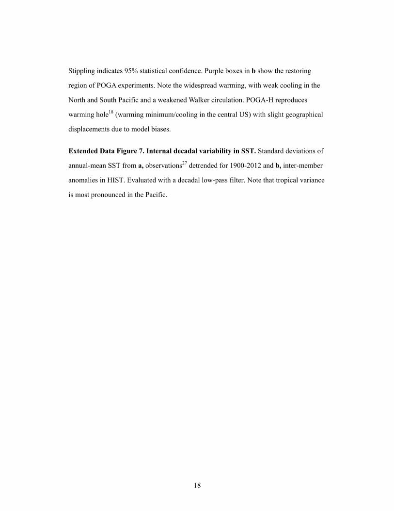
Stippling indicates 95% statistical confidence. Purple boxes in b show the restoring

region of POGA experiments. Note the widespread warming, with weak cooling in the

North and South Pacific and a weakened Walker circulation. POGA-H reproduces

warming hole18

(warming minimum/cooling in the central US) with slight geographical

displacements due to model biases.

Extended Data Figure 7. Internal decadal variability in SST. Standard deviations of

annual-mean SST from a, observations27

detrended for 1900-2012 and b, inter-member

anomalies in HIST. Evaluated with a decadal low-pass filter. Note that tropical variance

is most pronounced in the Pacific.

0.2

0.1

0

–0.1

–0.2

–0.3

–0.4

0.6

0.3

0

–0.3

–0.6

–0.9

–1.21950 1955 1960 1965 1970 1975 1980 1985 1990 1995 2000 2005 2010

0.7

0.6

0.5

0.4

0.3

0.2

0.1

0

–0.1

–0.2

–0.3

–0.4

–0.5

–0.6

–0.7

–0.8

b

DJF JFM FMA MAM AMJ MJJ JJA JAS ASO SON OND NDJ

c

Observed, HIST and POGA-H annual-mean anomalies [ºC]

POGA-C annual-mean anomalies [ºC]

Observed and POGA-H 2002-2012 seasonal-mean trends [ºC per 11 yr]

0.1

0

–0.1

–0.2

–0.3

POGA-HObservations

a

2002-2012 average

99 percentile

95 percentileensemble mean

Observations

HISTPOGA-H

POGA-HHISTObservations

Annual-mean global average

POGA-C5yr running mean

Restoring region SAT

El Chichon

Pinatubo

Agung

90ºN

60ºN

30ºN

0º

30ºS

0º 60ºE 120ºE 180º 120ºW 60ºW 0º

a b

c d

–9 –6 –4 –2 –1 0 1 2 4 6 9 hPa per 11 yr

Observed DJF T trends for 2002-2012 POGA-H DJF T trends for 2002-2012

Observed DJF SLP trends for 2002-2012 POGA-H DJF SLP trends for 2002-201290ºN

60ºN

30ºN

0º

30ºS

0º 60ºE 120ºE 180º 120ºW 60ºW 0º

0º 60ºE 120ºE 180º 120ºW 60ºW 0º 0º 60ºE 120ºE 180º 120ºW 60ºW 0º

–2.5 –2.2 –1.9 –1.6 –1.3 –1 –0.7 –0.4 –0.1 0.1 0.4 0.7 1 1.3 1.6 1.9 2.2 2.5ºC per 11 yr

–5 –4.5 –4 –3.5 –3 –2.5 –2 –1.5 –1 –0.5 0 0.5 1 1.5 2 2.5 3 3.5 4 4.5 5mm d–1 per 11 yr

90ºN

60ºN

30ºN

0º

30ºS

0º 60ºE 120ºE 180º 120ºW 60ºW 0º

a b

c d

Observed JJA T trends for 2002-2012 POGA-H JJA T trends for 2002-2012

Observed JJA precipitation trends for 2002-2012 POGA-H JJA precipitation trends for 2002-201290ºN

60ºN

30ºN

0º

30ºS

0º 60ºE 120ºE 180º 120ºW 60ºW 0º

0º 60ºE 120ºE 180º 120ºW 60ºW 0º 0º 60ºE 120ºE 180º 120ºW 60ºW 0º

–2.5 –2.2 –1.9 –1.6 –1.3 –1 –0.7 –0.4 –0.1 0.1 0.4 0.7 1 1.3 1.6 1.9 2.2 2.5ºC per 11 yr