recent mathematical tables 215 - american …€¦ · recent mathematical tables 215 5-point ... m...

RECENT MATHEMATICAL TABLES 215

5-Point

r = (A/,' - ßBo + Ím5o3)/A,

s = %ß803/A,

t = lS04/A, u = v = 0,

where A = 502 - tïoq*.

6-Point

r = (A/,' - ßd0 + |pôo3 - *Wo6)/A,

s = (hßoo3 - |mSo5)/A,

t = |5o4/A,

m = ttaôVA, i> = 0,

where A = 502 — tVô4.

7-Point

r = (Ä// - m5o + èiiao3 - ïV/i3o5)/A,

S = (fiiSo3 - |/uáo6)/A,

í = (|5o4 - ttWVA,

M = ÏT/i5o5/A,

» = xiirSoVA,

where A = 502 - tîô4 + îW-

H. E. SalzerNational Bureau of Standards

Washington 25, D. C.

This work was sponsored in part by the Office of Air Research.1 H. E. Salzer, "Table of coefficients for obtaining the first derivative without differ-

ences," NBS, Applied Mathematics Series No. 2, 1948.2 D. Gibb, A Course in Interpolation and Numerical Integration ¡or the Mathematical

Laboratory. London, Bell, 1915.3 H. E. Salzer, "A new formula for inverse interpolation," Amer. Math. Soc, Bull., v.

50, 1944, p. 513-516

RECENT MATHEMATICAL TABLES

915[F].—K. Früchtl, "Statistische Untersuchung über die Verteilung von

Primzahl-Zwillingen," Öster. Akad. Wiss., math.-nat. Kl., Anz., 1950,

p. 226-232.Information on the distribution of twin primes (p, p + 2) and quadruplets

(p, p + 2, p + 6, p + 8) is given for the first 1020000 natural numbers. Theinformation is based on the old table of Chernac.1 The main table gives the

number of prime pairs in each of the 1020 chileads 1000« < p < 1000(w + 1)for n = 0(1)1019. There is no chilead devoid of prime pairs and only

three (n = 688,851,927) with but a single prime pair. The rows of thistable are added to give the number of prime pairs in each of the 102 myriads

lOOOOra < p < 10000(» + 1) for n = 0(1)101. These frequencies are, inturn, added by tens to give a 10 entry table for each interval of 100000. The

grand total gives 8168 prime pairs < 106.

216 RECENT MATHEMATICAL TABLES

As for the quadruplets, there are enumerated in each of the 10 intervals

of 100000; the total number is 166. On p. 232 the largest quadruplet, p + 8,is given for each of the 172 cases below 1020000.

Previous tables concerning twin primes are mentioned in MTAC, v. 4,

p. 84. The reviewer has not as yet attempted to reconcile discrepancies

between these and the tables under review. No doubt some of these are due

to errata in Chernac.D. H. L.

1 L. Chernac, Cribrum Arithmeticum etc., Deventer, 1811.

916[I, O].—R. E. Beard, "Some notes on approximate product integration,"

Inst. of Actuaries, Jn., v. 73, part II, 1948, 356-403.

The author studies approximation formulas of the form :

j(x)tp(x)dx = CZ! cLrf(xr)] • 1 <f>(x)dx + P„ I <p(x)dx,Ja r=l Ja Ja

a < Xx, x2, ■ ■ -, xn < b, where the ar, xT are independent of f(x) and

Jah 4>(x)dx 9e 0. 4>(x) is generally a known, tabulated function and f(x) is a

complicated or empirically given function. One of the more important appli-

cations of such formulas is the evaluation of continuous single premiums

in the field of life and disability contingencies where <¡>(x) = vx is the dis-

count factor and f(x) is derived from a mortality or disability table for one

or more lives.

The paper is divided into two parts: a theoretical part in which formulas

are developed for the determination of a„ xr and the remainder term Rn, and

a part containing tables for the ar and xr based on the formulas of the first

part for low orders (i.e. small n).

In the theoretical part the following cases are considered :

(1) Neither the aT nor the x, are given; R„ depends on ß2n)(x).

(2) ax = a2 = • • • = an = ~ ; Rn depends on /(n+1)(;e).

(3) n = 3, ax = a3; R3 depends on flS)(x).

(4) The xT are given, P„ depends on fln)(x).

If nii = fab xl4>(x)dx/'fab <j>(x)dx are the moments of #(x) which are

assumed to exist and to be known, the xr in the cases (1) and (2) are found

to be the roots of a polynomial of degree n whose coefficients are determi-

nants the elements of which are multiples of the moments rrii. In the cases

(1) and (4) the ar are expressed as quotients of two determinants whose

elements depend in a simple manner on the xT and the »!¡. Simpson's rule,

Weddle's and Hardy's formulas are examples of formulas belonging to

case (4).In deriving his formulas for the remainder term Rn the author makes

an application of the mean value theorem which is correct only if <¡>(x) is

non-negative and 0 < a < b and arrives thereby at an expression for P„ of

the form /(i)(£i) ~n — fw(ii)h(xx, • • -, xr) where A has the values indicated

above, h(xx, ■ • ■, xr) is a function of the xT only which in many cases can


be expressed as a simple function of the mi, and 0 < £1, £2 < b. He then

simplifies this expression by stating that, for practical purposes, £1 and £2

may be replaced by a common value with 0 < £ < b which is evidently

correct only in particular cases. The remainder terms given by the author

are therefore useless in many cases for the purpose of measuring the accu-

racy of the approximation formulas. It is, in any event, doubtful whether

remainder terms expressed by means of derivatives of high order are useful

for empirically given functions f(x).

The author proceeds to develop from the general formulas the formulas

corresponding to low values of n. In many cases he first makes a linear

transformation of the variable ïtoa variable X so as to make «i = 0 and

m2 = 1 and then expresses the remaining moments by means of Pearson's ß(.

In those formulas where ßi for i > 3 appear he makes the further assump-

tion that the )3¡ for i > 3 can be expressed as functions of /3i and ß2 in the

same manner as for Pearsonian distribution functions.

In another special application the author considers special functions (p(x)

such as 4>(x) = 1, er*», exp (- {(x — m)/c)2), (1 — x)mi(l + jc)"*2.

No attempt has been made to classify the various formulas by some

optimum properties or by the magnitude of the remainder terms, the only

test being a comparison of the true values of some actuarial functions with

the results of various approximation formulas.

In the numerical part of the paper the following tables are given :

Table 1 : Solutions to 6D for Xx, X2, ax, a2 for the two point formulas of

case (1) corresponding to ßx = 0(.1)3.0(. 1)3.0.

Table 2 : Solutions to 6D for Xx, X2, X3, ax, a2, a3 for the three point for-mula of case (1) corresponding to ßx = 0(.2)2 and ß2 = 2(.5)6.

Table 3: Solutions to 6D for Xx, X2, X3 for the three point formula of

case (2) corresponding to ßx — 0(.01).50.

1 ATable 4: Solutions to 6D for Xx, X2, X3, ax = a3 = -z——j, a2

2+A'"' 2+Afor case (3) corresponding to ßx = 0(.2)2 and ß2 = 2.0(.5)6.0.

Table 5: Moments mx, m2, m3, <j to 3D and 'sßx to 5D for the continuous

function (1 + i)~x for * = .02(.01).06 and n = 5(5)60.Table 6: A similar table for discrete moments.

Table 7: Solutions to 5D for ax, a2, a3 for the three point formula of case

m(4), where Xi = 0, x2 = — , xm = m and 4>(x) = (1 + i)~x for m = 5(5)50

and * = .02(.01).06.Table 8: The values to 3D of ex, ëxx, ëxxx, ëxxxx, ëxxxxx for the A 1924-29

ultimate mortality tables for x = 15(1)80.Table 9: <r to 3D, (/Si)* to 5D, 182 to 4D for the function (ßl)xx... for 1 to

5 lives of the A 1924-29 ultimate mortality table.

There are also a few auxiliary tables for the purpose of evaluating re-

mainder terms.

Stefan Peters

University of California

Berkeley, California

218 recent mathematical tables

917[I].—Leroy F. Meyers & Arthur Sard, "Best approximate integration

formulas," Jn. Math. Phys., v. 29, 1950, p. 118-123.

For each A = c0x(0) + Cxx(l) + ■ • • + cmx(m) that is an approxima-

tion to fomx(t)dt which is exact whenever x(t) is a polynomial in / of degree n,

m > 1, n > 0, there is a kernel function k(t) such that, when x(t) is of

class Cn+1,

x(t)dt - A = x^+»(t)k(t)dt.o Jo

The kernel function is defined explicitly by

k(f) = 2?r>,,] = - *[>,.]where

/ t lt\ \ ° a. a. (,\ /(' -t'Y/n\ Ht<t'h, = Mt) = | {t _ t,)n/nl 4». = Mt) = | 0 ut>i,

By Schwarz's inequality

I^MI < ( Jmk2(t)dt\ (\mx(»+»(tydt).

The best approximation A, for given m and n, is defined as that which

minimizes J as f0mk2(t)dt.

In the present paper, the authors give the best integration formulas for

n = l, m = 1(1)20; n = 2, m = 2(1)12; n = 3, m = 2(1)9. For thesevalues of n and m, they tabulate the exact values of c0, C\, ■ • -, cm and /.

In an earlier paper by Sard1 the best integration formulas are given for

n = 0, all m, and n = 1, 2, 3, m < 6.The authors derive some fundamental algebraic relationships between

the Ci's and J. Then for the case n = 1, recursive relations are derived

which afford a complete characterization of the best integration formulas

for any m. Finally, the authors give some conjectures about the con-

vergence of the coefficients, some of which are true for n = 0 and 1, but

which are open questions for n > 2.

H. E. SalzerNBSCL

1 A. Sard, "Best approximate integral formulas; best approximation formulas," Amer.Jn. Math., v. 71, 1949, p. 80-91.

918[I].—Leroy F. Meyers & Arthur Sard, "Best interpolation formulas,"

Jn. Math. Phys., v. 29, 1950, p. 198-206.

The tabular values x(0), x(l), x(2) of a function x(t) being given, the

problem discussed here is the approximation of x(u) by an expression of the

form A = a0^(0) + axx(l) + • • • + amx(m), where the value of m and the

coefficients a0 = a0(u), ax = ai(u), • ■ -, am = am(u) are to be determined.

If A is an exact approximation whenever x(t) is a polynomial of degree n,

there is a kernel function k(t, u), such that when x(t) is of class Cn+l,

PC*] = x(u) - A = \ x^+»(t)k(t, u)dt,Jk


where K is the smallest interval containing u and those values of 0, 1, ■ ■ ■ ,m

for which the corresponding aa, ax, • ■ •, am are not zero. For each u, k(t, u)

is a broken polynomial in / consisting of at most m + 3 arcs, which is defined

explicitly by

k(t', u) = Rfytq = - Rl4>,>],

where

,, f 0 ., \(t-t'Y/n\ iît<t',** = MO = j {t _ 0„M ** = MD = ( 0 {it>t,

By Schwarz's inequality

I-KM I < À J xi»+»(t)'dt/\K\

where the modulus M is defined by M = M(u) = £\K\fKk(t, w)2d/J*. Forgiven m, n, u, that A is called best which minimizes the modulus M, and

it is denoted by Am,n,u. The authors report that for n = 0, all m, and n = 1,

m = 1(1)4, n = 2, m = 2, the conventional polynomial interpolation is

best, but not for n = 2, m = 3, 4, 5.The determination of Am,„,u involves the prior determination of a num-

ber of approximations Pm,„,„ (for different values of m and u) where Pm,„,u

is that A which minimizes / = SZmÏ/mW, u)2dt. The modulus of Bm,n,u is

denoted by Mm¡n¡u.

The authors tabulate the auxiliary function ß = Ml,.2,u/d(u) where

6(u) = (u- [u])2(l -u+ Cw])2/120form = 2(1)5,« = 0(.l)2;w = 3(1)5,u = 2.1(.1)2.5 ; 2D. The table of ß enables one (a) to compare moduli,

(b) to identify Am+j,%u with Bm,2|U, 0 < 5 — m, where each different value

of m corresponds to a different range of u, and (c) to find the proper argu-

ment by translation in using the main table..

The principal table in the article is the collection of formulas for Pm, 2, u,

0 < u < [_(m + l)/2], m = 2, 3, 4, and M^a.«, u < [(m + l)/2],m = 2, 3, 4, 5. In the Bm, %u, the coefficients of xo, xx, • • • ,xm are given as

exact polynomials in u. The M^, 2,„ are expressed as either exact poly-

nomials in u, or as exact polynomials in u multiplied by 6(u). The expres-

sions for Bm,2,u and M2m¡2,u are different for u lying within different ranges.

The rest of the paper is concerned with the derivation of those formulas

and their transformation under a linear transformation of the /-axis,

t* = bt + c, b 5¿ 0.H. E. Salzer

NBSCL

919[J].—T. M. Cherry. "Summation of slowly convergent series," Camb.

Phil. Soc, Proc, v. 46, 1950, p. 436-449.

This paper studies two transformations of the remainder that are helpful

in numerical summations.00 00

The power series considered is £ CrtT, and, in the remainder £ CrtT,0 n

Cr is written as a product crf(r), where it is supposed that f(z) has an

asymptotic expansion

f(z) ~ Aza + AxZai + A2zai + • • ■


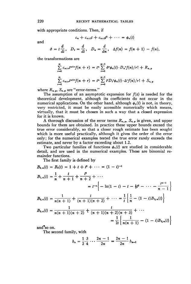
with appropriate conditions. Then, if

£„ + cn+xt + cn+2t2 + ■ ■ ■ = (j>„(t)

and

»-"î* D»mi* D» = £> A/(«) -/(» + 1) -/(«),

the transformations are

£ cn+rtn+rf(n + r) =t" £ &r*n(t)-Dsf(n)/rl + Rn,Pr-0 r—0

£ cn+rt*+'f(n + r) = /»E t'Df<t>n(t)-A*f(n)/r\ + Sn,pr=0 r=0

where Pn.P, Sn,P are "error-terms."

The assumption of an asymptotic expansion for f(z) is needed for the

theoretical development, although its coefficients do not occur in the

numerical applications. On the other hand, although <bn(t) is not, in theory,

very restricted, it must be easily accessible numerically which means,

virtually, that it must be chosen in such a way that a closed expression

for it is known.

A thorough discussion of the error terms P„,p, Sn.P is given, and upper

bounds for them are obtained. In practice these upper bounds exceed the

true error considerably, so that a closer rough estimate has been sought

which is more useful practically, although it gives the order of the error

only; for the numerical examples tested the true error rarely exceeds the

estimate, and never by a factor exceeding about 1.2.

Two particular families of functions <j>n(t) are studied in considerable

detail, and are used in the numerical examples. These are binomial re-

mainder functions.

The first family is defined by

Bo,n(t) = B0(t) = 1 + / + t2 + ■ ■ • = (1 - i)"1

B^=í + nJri+nJh+---= r- j - in(i - t) - t - \t2-^y

*■<*> -n^+T) + (n+lKn + 2) + ' ' ' " j{ I ' (1 " t)BUt)\

_1_ _t_B*n(t) = n(n + l)(n + 2) + (n + 1)(« + 2)(n + 3) + '"

= Í\n^+T) - ^ - t)B^and"so on.

The second family, with

1 3 2w - 1 2n - 16" = 2-4-2n~=~^n~b"-1


is given by

Bi,n(0 = bn + bn+xt + bn+2t2 4

= ¿"»{(I - i)"* - 1 - ¥ - • • • - bn-xt"-1}

*.W-;Hh + i^+"—îi*.-a-«*.wi

- (1 - t)Bln(t)\n + 1

i'nW (n + 1)(» + 2) T (n + 2)(n + 3) T "

2" 3/

and so on. w

Tables are given of Bj,M(i) = £ &10+.Í" = R(r, 6) + î/(r, 0) to 4 decimalss=0

for r = 0.7(0.05)1, 6 = 0°(5°)90°, and have been used for the numericalexamples, which concern the Kapteyn series

00

£ xrJr(ry)T=X

and are very fully considered.

J. C. P. MillerUniversity Mathematical Laboratory

Cambridge, England.

920[K, L].—B. V. Gnedenko, Kurs Teorii Veroiàtnostei [A Course in the

Theory of Probabilities]. Moscow and Leningrad, 1950, 388 p.

On p. 372-385 there are tables of

4>(x) = 4= e-*1'2, x = C0(.01)3.99; 4D]\2x

$(*) = -= )* e-'*i*dz, x = 0(.01)2(.02)3(.2)4(.5)5; 4D up to 2.98,

5D to 8D thereafter

Pk(a) = ^f , a = .1(.1)1(1)9, A = [0(1)27; 6D]

k am(e-°)£^V> a = .1(.1)1(1)3, A = [0(1)15; 6D]m=o m\

P^ = -1 /b\ ) zk-le-*l2dz, x = 1(1)30, A = [1(1)29; 4D]2(i-2)/2p |

ris(x) = —''® r(1+-*-\

n/2

dz

n = 2(1)20, oo, x = [0(.1)6; 3D], * - oo ; 5D


K(x) = £ (- l)*e-2*2*2, x = .28(.01)2.50(.05)3; mostly 6Dfc=—oo

,1-/3In-

a

Brown University

Providence, Rhode Island

921[L].—Aircraft Radiation Systems Laboratory, "Tables of modified

cosine-integral," Stanford Research Institute, 1951, viii + 56 p.

These tables contain 6D values of

7^. , x f* 1 - COS Í ,Ci (x) = -;-dt

Jo t

for x = 0(.001) 10(.01)50. The computation was carried out, largely on

IBM machines, by the Telecomputing Corporation of Burbank, California.

The introduction, by C. T. Tai, discusses the connection of Ci with the

cosine-integral function and the application of the tables, and describes the

computation and preparation of the tables. A bibliography is appended.

The work was sponsored by the U. S. Air Force.

A. E.

922[L, M, Q, S].—M. P. Barnett & C. A. Coulson, "The evaluation ofintegrals occurring in the theory of molecular structure. Parts I and

II," Roy. Soc. London, Philos. Trans., v. 243A, 1951, p. 221-249.

Table 1, p. 233. Modified Bessel functions of the first kind, In+i(x),to 7S for n = - 1(1)4 and x = .5 (.5) 10.

Table 2, p. 233. Modified Bessel functions of the third kind, Kn+\(x),to 7S for n = - 1(1)4 and x = .5(.5)10(1)25.

These tables are used for the numerical computation of the functions f

defined by the expansion

„mr-lg-, = (¿r)-i ¿ (2« + l)Pn(cOS 0)fm,n(l, t; r)n=0

where r2 = t2 + t2 — 2tr cos d. With these functions the authors form

Xooe-"Un(l, t;T)t'+idt

and discuss the computation of Z by both numerical integration and ana-

lytical methods.In the memoir it is shown that a large number of integrals occurring

both in nuclear physics and astrophysics can be reduced to known integrals

and to Z integrals. Formulas are listed for more than 180 integrals.

A. E.

923[L].—C. L. Bartberger, "The magnetic field of a plane circular loop,"

Jn. Appl. Phys., v. 21, 1950, p. 1108-1114.

a = .001, .01(.01).05, .1, .15

ß = [.001, .01(.01).05, .1, .15; 3D]R. C. Archibald


The integrals

J, = x-i I (1 - b cos 6)~idd

I2 = x"1 I (1 — A cos 0)-* cos 0d0

are expressed in terms of complete elliptic integrals. Series expansions are

also given in ascending powers of b and 1 — b.

Table I (p. 1110-1111) gives 6D values of Ix, and table II (p. 1111-1112)6D values of h, for b = 0(.001).809.

Table III (p. 1113-1114) gives 6D values of h, I2, Ix - 1% (1 - b)Ix,(1 - b)I2 for b = .8(.001)1, and table IV (p. 1114) 6D values of the samefunctions as table III for 6 = .995(.0001)1.

A. E.

924[L].—A. Fletcher, "Tables of two integrals and of Spielrein's inductance

function," Quart. Jn. Mech. Appl. Math., v. 4, 1951, p. 223-235.

The tables (p. 229-232) are of

/ = P (K - E)dk, J = V (K - E)k~3dkJa Ja

and -16ir(7 - ct3J)/[3(l - a)2].

Values are given to 10D, 10D and 6D respectively. The range of a is

0(.01)1. Half a dozen small auxiliary tables are also given.

925[L].—Harvard University, Computation Laboratory, Annals, v. 14:

Tables of the Bessel Functions of the First Kind of Orders Seventy-Nine

through One Hundred Thirty-Five. Cambridge, Mass., Harvard Univer-

sity Press, 1951, viii, 614 p. 19.5 X 26.7 cm. $8.00.

This is the twelfth and final volume of the monumental set of Tables of

Bessel Functions of the First Order, published by Harvard during the past

five years—six volumes in 1947, three in 1948, two in 1949 and one in 1951.

The tabular parts of the volumes fill 7652 pages. The previous 11 volumes

have been reviewed in MTAC: v. 2, p. 261-262, 344; v. 3, p. 102, 185-186,367, 474-475 ; v. 4, p. 22, 92. Roughly speaking we now have here 10Dtables of all J„(x), for x = 0(.01)100, when n = 0(1)111 ; and for x = 0(A)-100, when n has any positive integral value > 111 ; for n > 135 the values

of Jn(x) are always less than 10-10. In addition to what is thus stated, for

n = 0(1)3, x = C0(.00l)25(.01)100; 18D]; for n = 4(1)15, x = C0(.001)-25(.01) 100; 10D]. Detailed information concerning interpolation in the

whole range is given in Annals, v. 3 and 5 ; for 10D interpolation the work

is not excessive.

Further, in the present volume we have 10D tables of Jn(n) for n = 0(1)-

100. Zero values are not given, since the values found by the Computation

Laboratory were presented to the Royal Society Committee for use in

connection with their second volume of Bessel function tables. For n>92,

x<100, Jn(x)^0. For Jn(n), in the Harvard range, we had earlier: Meissel

(1891), n = 20 to 20D; Meissel (1895), n = 1(1)24 to 18D; Airey (1916),


n = 1(1)50(5)100 to 6D; Watson (1922), n = 1(1)50 to 7D; and Hayashi(1930), n = 2 to 101D, n = 10 to 61D, n = 20 to 41D, n = 30 to 35D,n = 40 to 35D, n = 50 to 30D, n = 100 to 18D. Hence most of the valuesin this special Harvard table are new.

In the recent Russian table of Faddeeva and Gavurin, RMT 852, the

argument extends to 124.9, at interval .1, so that some 6D of Jn(x) for all

orders, n = 0(1)120 supplement values given in the Harvard tables. So also

for 5D zeros < 125, of Jn(x) ; the last zero is for Jxxs(x).

The remarkable Automatic Sequence-Controlled Calculator on which

these tables were computed carried the values of Jn(x), for n = 0(1)3 to

23D, and for n > 3 to not less than 13D and most of the time much more

than this; its electromagnetic typewriters also wrote out, for checking

purposes, 10 differences in every case, and also finally produced the 18D

or 10D copy which could be sent directly to the printer for offset repro-

duction. The computation of these tables was only a tiny fraction of the

work achieved in the ASCC since its activities began in 1945, and have

continued to the present, 24 hours a day, 7 days a week.

Only one tabular slip has ever been found in the published volumes,

73(72.10) \_MTAC, v. 3, p. 41], but this slip was due to some reproductiondifficulty, and not to any error in computation or in automatic mechanical

checking. In the last line of the second page of the "Preface," of the volume

under review, for J(x), n = 0(1)120, x = C0(.01)14.99; 8D], read Jn(x),n = 0(1)120, x = C0(.l)124.9; 6D]; n = 0(1)13, x = C0(.01)14.99; 8D].

In the first page of the Preface, line — 2, for Claire, read Clare.

These Harvard Bessel Function tables, with most of the values new,

constitute an outstanding contribution to scientific research.

R. C. Archibald

Brown University

Providence, Rhode Island

926[L, S].—Helmar Krupp, "Bestimmung der allgemeinen Lösung der

Schrödinger-Gleichung für Coulomb-Potential," Akad. Wiss. Leipzig,

mat.-phys. KL, Berichte, v. 97, 1950, no. 8, p. 1-28.

The Schrödinger equation for the Coulomb potential is

d2R 2dR T 1 1 /(/ + 1) "I „ , „ . „^ + ;¿7 + 2L-^ + r-^-r = 0, / = 0'1'2'---

Two solutions are written in the form

(2r)1yP(«, I, r) = + ^ er*'» ¿M(a, b, x), j = 1,2,

where a = Z + 1 — n, b = 21 + 2, x = 2r/n.With the abbreviations

(a)o = 1, (a)m = a(a + 1) ■ ■ ■ (a + m — 1) for m = 1, 2, • • •A = tf(-a) if a = 0, -1, -2, •••A - *(a - 1) if a 91 b - 1, b - 2, • • ■


the definitions of the M are

xM(a, b,x) = £ g^m_o (b)mml

ir 2M(a, b, x) = [In x + C - *(& - 1) + A] xM(a, b, x)

+ » (a)mx^ m£ ( 1_1_1_\

m_i (b)mm\ ¡fc=o\a + A b + k 1 + A /

+ £ v ', s T(a - b + m + l)bl(b - m - 2)\xm+l-\m=om\T(a)

Tables are given for iP, dxR/dr, 2R, d2R/dr for 0 < x < 15 (the interval

in most cases is .5), for I = 0 and » = -(-!-, / = 1 and n = -( - 1 - ,

1 = 2 and n = — ( - j - . Graphs of these functions are added. A misprint

occurs on page 14, line 3 from the bottom and on page 15, line 6; in both

places ( J should be replaced by I 1 . However

the formulas to which the author refers as the source of computation do not

contain this misprint.

Maria Weber

California Institute of Technology

Pasadena, California

927[L].—U. E. Kruse & N. F. Ramsey, "The integral Jo00 y3 exp ( - y2

+ ix/y)dy," Jn. Math. Phys., v. 30, 1951, p. 40-43.

In several problems of theoretical physics there arise integrals which can

be reduced to the real part, I(x), or the imaginary part, K(x), of. the integral

mentioned in the title. Table 2 of this paper gives 5D values of both these

functions for * = 0(.1).4(.2)8(.5)20.Convergent expansions, useful for x < 3, have been given by Zahn,1

and Table 1 of the present paper gives numerical values, to 7-9S, of the

coefficients up to that of x14. For larger x it is more convenient to use asymp-

totic series developed by Laporte,2 and 6D values of the first six coefficients

in these series are also given in the present paper. [The author remarks

that in Torrey's paper3 the recurrence formula for the coefficients contains a

misprint, but Torrey's numerical values are in agreement with the author's.]

Table 2 was computed from these expansions, and V. E. Culler assisted

in the computation.

A. E.

1 C. T. Zahn, "Absorption coefficients for thermal neutrons," Phys. Rev., v. 52, 1937,

p. 67-71.2 O. Laporte, "Absorption coefficients for thermal neutrons," Phys. Rev., v. 52, 1937,

p. 72-74.' H. C. Torrey, "Notes on intensities of radio frequency spectra," Phys. Rev., v. 59,

1941, p. 293-299.


928[L, S].—N. Metropolis & J. R. Reitz, "Solutions of the Fermi-Thomas-Dirac equation," Jn. Chem. Phys., v. 19, 1951, p. 555-573.

Solutions \p are given of the equation

d2é■jZ = x(e + fa-*)3 (e3 = 3-2-6-ît-2Z-2)

in terms of the variable w = (2x)*. The tables are at intervals of .08 and

extend until \f/ becomes negative. The parameter Z takes on the 24 values

Z = 6(4) 14, 16, 18 (4) 26, 29 (4) 81, 84 (4) 92

and there are 8 different initial slopes ip'. Actually 2\f/ is tabulated to 5D.

The calculations were done on the EN I AC.D. H. L.

929[L].—L. Prandtl, with the assistance of F. Vandrey, "Flieszgesetze

normalzäher Stoffe im Rohr," Zeit, angew. Math. Mech., v. 30, 1950,

p. 169-174.Table 1. 4S table of

<p(a) = | cosh a — — sinh a + — (cosh a — 1)¿iCL Or

fora = 0(.1)5(.2)10.Table 2. 3D table of v(aÇ) / <p(a) îor t = 0(.2).6(.1)1 anda = 1(1)10(2)14.

Some of the values were obtained by interpolation: these are put in paren-

theses.A. E.

930[L].—S. Silver & W. K. Saunders, "The radiation from a transverse

rectangular slot in a circular cylinder," Jn. Appl. Phys., v. 21, 1950,

745-749.Table I gives values of ka, n, and <p0 for which H0™'(ka)/Hnm'(ka) < .0001

and (w0o)_1 sin n<j>Q > .9.

Table II gives 4D values of

" 6„t" cos n<t> I "

h sin 0Hnv'(ka sin 0)/ to

tnln

Hn^'(ka)

iorka = .8, 0 = 10°(10°)90°, <t> = 0°(10°)180°. Here e0 = 1, e„ = 2 if « > 0.Table III is similar to table II except that ka = 2.5.

A. E.

931[L].—E. Wolf, "Light distribution near focus in an error-free diffraction

image," Roy. Soc. London, Proc, v. 204A, 1951, 533-548.

In the course of the work the function

2m

©■«(«O = E (- l)°lJs(v)J2m-a(v) + Js+x(v)j2m+x-s(v)]s-0

is introduced, where the / are Bessel functions of the first kind.


Table 1 (p. 541) gives 5D values of Q2m(v) for v = 0(1)15 and m = 0(1)M(v) where

M(v) = v +1 for v < 5, M(6) = 6, M(7) = M(B) = 7, M(9) = 8,M(10) = M(ll) = 9, M(12) = 10, M(13) = M(14) = 11,

and M(15) - 12.

The results of some numerical computations involving these functions

are given in form of diagrams.

A. E.

932[V].—E. Gruschwitz, Calcul approché de la couche limite laminaire en

écoulement compressible sur une paroi conductrice de la chaleur. Office

National d'Études et de Recherches Aeronautiques (O.N.E.R.A.). Pub-

lication No. 47, Chatillon-sous-Bagneux, Seine. 1950, 39 p.

As a generalization of the Kármán-Pohlhausen1 method to steady

compressible flow, the velocity component u parallel to a wall y = 0 is ap-

proximated within the boundary layer by a quartic in r¡ = const So" pdy

for a fixed x; moreover, the density p is expressed as a rational function of r¡.

These assumptions lead to the system :

(1) (6ue/Ve)de/dx = Fx(K) - (K/b0)[2 - M2F2(k)2,

(2) bo = (1 + .2025 M2)[l + M2F3(K)y[l + M2F,(k)],

(3) K = (62bo/ve)due/dx,

with known initial conditions at ue = 0 for the determination of K (which

is a quintic in Pohlhausen's parameter X), b0 = CPe/p]i-o, and the momentum

loss 0 = fov'(pu/peue)(l — u/ue)dy. The velocity ue, kinematic viscosity ve,

Mach number Me and density pe are supposed known in the main stream

as well as ye = C30»=.99«e> while the functions F¡(K), which depend on the

Prandtl number Pr, are tabulated to 3D (i = 2, 3, 4) or 4D (i = 1) forK = .094(-.001) - .156 CPr = .725 (i = 1, 2, 3, 4) and Pr = 1 (i = 2)].In addition the displacement 8* = Jo"' (1 — pu/peue)dy of the main stream

from the wall is given by Ô* = 6[bofx(K) + M2f2(K)], the ft(K) beingtabulated to 3D for the above range in K [Pr = .725].

In the appendix E. A. Eichelbrenner describes an exact method and

presents graphical results indicating that certain aerodynamical quantities

(excluding the temperature) are equally well approximated by using

Pr = .725 or the simpler value Pr = 1 [F3(K) = P4(P)] in Gruschwitz'smethod.

The tables on pages 13-16 have columns of values of K (as above),

X (generally to 4S), P3, Ft, fx, f2, Pi, P2, F2 CPr =1]- There are also rowsof values for X = ± 12, 7.0523, K = - .157 (X, Pi, P2, P2 CPr = 1]).

The identities P2 = .595 + P3 and /2 = .405 — P3 should hold through-out the table.

R. R. ReynoldsNational Bureau of Standards

Institute for Numerical Analysis

Los Angeles 24, California

1 K. Pohlhausen, "Zur näherungsweisen Integration der Differentialgleichungen derlaminaren Grenzschicht." Zeit, angew. Math. Mech., v. 1, 1921, p. 252-268.

recent mathematical tables 215 - american …€¦ · recent mathematical tables 215 5-point ... m...

Documents