1

Reciprocal trade agreements in

gravity models: a meta-analysis

Maria Cipollina (University of Molise, Italy) and Luca Salvatici (University of Molise, Italy)

Working Paper 06/12

TRADEAG is a Specific Targeted Research Project

financed by the European Commission within its VI

Research Framework. Information about the Project, the

partners involved and its outputs can be found at

http://tradeag.vitamib.com

University of Dublin

Trinity College

Reciprocal trade agreements in gravity models: a meta-analysis

Maria Cipollina and Luca Salvatici∗∗∗∗

(University of Molise)

Abstract

Over the time a large number of reciprocal preferential trade agreements (RTAs) have been

concluded among countries. Recently many studies have used gravity equations in order to estimate

the effect of RTAs on trade flows between partners. These studies report very different estimates,

since they differ greatly in data sets, sample sizes, and independent variables used in the analysis.

So, what is the “true” impact of RTAs? This paper combines, explains, and summarizes a large

number of results (1827 estimates included in 85 papers), using a meta-analysis (MA) approach.

Notwithstanding quite an high variability, studies consistently find a positive RTAs impact on

bilateral trade: the hypothesis that there is no effect of trade agreements on trade is easily and

robustly rejected at standard significance levels. We provide pooled estimates, obtained from fixed

and random effects models, of the increase in bilateral trade due to RTAs. Finally, information

collected on each estimate allows us to test the sensitivity of the results to alternative specifications

and differences in the control variables considered.

JEL classification: C10; F10.

Keywords: Free Trade Agreements; Gravity equation; Meta-regression analysis; Publication bias.

∗ This work was in part financially supported by the “Agricultural Trade Agreements (TRADEAG)” project, funded by the European Commission (Specific Targeted Research Project, Contract no. 513666); and in part supported by the Italian Ministry of University and Technological Research (“The new multilateral trade negotiations within the World Trade Organisation (Doha Round): liberalisation prospects and the impact on the Italian economy”).

2

1. Introduction.

Preferential agreements are discriminatory policies entailing trade liberalization with respect

to a subset of trading partners. The world trading system is characterized by a wide variety of

preferential agreements, which can be broadly categorized into two major types: reciprocal

(bilateral), entailing symmetric trade liberalization, and nonreciprocal (unilateral), entailing

asymmetric trade liberalization aimed at providing support to the country which gains improved

market access without being required to open up its own domestic market. The latter, as it well

known, have been widely utilized as an instrument for integrating the developing countries into

the world trading system.

Traditionally, reciprocal preferential agreements occurred between geographically

contiguous countries with already established trading patterns. However, the configuration of

these agreements is presently diverse and becoming increasingly complex with overlapping

agreements spanning within and across continents in what Bhagwati calls a “spaghetti bowl” of

trade relationships.1 The world has witnessed a veritable explosion of reciprocal preferential

trade agreements (RTAs) in the past 15 years. More than half of world trade now occurs within

actual or prospective trading blocs, and nearly every country in the world is a member of one or

more agreements (Clarete et al., 2003).

RTAs take many forms. The most common are the free trade area (FTA)—where trade

restrictions among member countries are removed, but each member maintains its own trade

policies towards nonmembers—and the customs union—a FTA where members adopt a

common external trade policy. Deeper forms of integration include a common market—a

customs union that also allows for the free movement of factors of production—and economic

unions, which involve some degree of harmonization of national economic policies. New RTAs,

indeed, place considerable emphasis on liberalisation of services, investments and labour

markets, government procurement, strengthening of technological and scientific cooperation,

environment, common competition policies or monetary and financial integration.

In the literature there are numerous studies analysing the economic impacts of RTAs. The

focus of this paper is on estimates of the effects on trade. RTAs might be expected to increase

trade between partners, since cheaper imports within the agreement may replace domestic

production –trade creation – or crowd out imports from the rest of the world – trade diversion

(Viner, 1950; Meade, 1955). However, intra-agreement trade flows may increase even before the

formal signature of the agreement, the increases reflecting the impact of unilateral and

1 As a consequence we decided not to use the term “regional”, which is traditionally used as a convenient shortcut, but is inconsistent with the plethora of agreements linking countries around the globe.

3

multilateral liberalization, as well as the simple fact that agreements may be due to, rather than

allow for, growing trade relationships.2

The purpose of this review is to use a Meta-Analysis (MA) approach to summarize and

analyse the RTAs trade effects estimated in the literature, mostly through gravity models

assessing the difference between potential and actual trade flows (see Appendix 1 for details on

the agreements considered). The approach takes as individual observations the point estimates of

relevant parameters from different studies. An MA can improve the assessment of the parameter

describing the RTAs impact by combining all of the estimates, investigating the sensitivity of the

overall estimate to variations in underlying assumptions, identifying and filtering out publication

bias, and by explaining the diversity in the study results in relation to the heterogeneity of study

features through meta-regression analysis (MRA).

In this paper, we firstly consider all point estimates provided in the literature, i.e. including

multiple estimates coming from a single study. We test for correlation within and between

studies, and estimate meta-regression models using weighted least squares (WLS), checking the

robustness and sensitivity of our results. Then, we focus on the effect on bilateral trade of

specific trade agreements. Finally, we run a probit regression in order to assess what are the most

important factors explaining a positive (and significant) impact of the agreements on bilateral

trade flows.

The paper is structured as follows. In Section 2 we briefly review the literature studying the

impacts of RTAs on trade, while in Section 3 we present some methodological issues regarding

the MA approach. In Section 4 we discuss the explanatory variables and present the econometric

results. Finally, Section 5 concludes.

2. The impact on trade of reciprocal preferential trade agreements

Empirical research applies econometric approaches to historical trade data in order to assess

the impact of trade agreements on bilateral trade flows. Usually, these approaches use gravity

models, based upon Newton’s Law of Gravitation, predicting that the volume of trade between

two economies increases with their size (proxies are real GDP, population, land area) and

decreases with transaction costs measured as bilateral distance, adjacency, cultural similarities

(Baldwin, 1994; Eichengreen and Irwin, 1996; Feenstra, 1998; Anderson and van Wincoop,

2003).

The standard formulation expresses the bilateral trade between country i and country j as:

ijijjiij εDistβYβYββT ++++= )ln()ln()ln(ln 3210 (1)

2 Also in the case of multilateral agreements, recent empirical work (Rose, 2004) does not find significant differences between the trade patterns of countries before and after their accession to the GATT/WTO.

4

where Tij is the country pairs’ trade flow, Yi(j) indicate GDP or GNP of i and j, Distij is the

distance between i and j, finally εij is the error term. Most applications of the gravity model

search for evidence of actual or potential effects by adding dummy variables for common

languages, for common land borders and for the presence or absence of a RTA. Then, the gravity

model is estimated as:

ijijijijijjiij RTALangAdjDistYYT εγββββββ +++++++= 543210 )ln()ln()ln(ln (2)

where Adjij is a binary variable assuming the value 1 if i and j share a common land border and 0

otherwise, Langij is a binary variable assuming the value 1 if i and j share a common language

and 0 otherwise, RTAij is a binary variable assuming the value 1 if i and j have a reciprocal trade

agreement in place and 0 otherwise. A positive coefficient for the RTA variable indicates that it

tends to generate more trade among its members. In MA, the parameter of interest (estimate of γ)

is commonly referred to as the “effect size”.

Many papers find positive and statistically significant RTAs dummies, although they are not

primarily interested in estimating the RTA effect, i.e. the existence of an RTA is only included as

a control variable. On the other hand, if there is a particular interest on specific RTAs, different

dummies may be introduced for each agreement.

Some authors distinguish between the increase in the volume of trade within the bloc and the

decrease in trade from countries outside the bloc (i.e., trade diversion) by including two dummies

for intrabloc and extrabloc trade. An example of a gravity equation that takes into account the

trade creation and diversion effects is:

ijjkikijijijijjiij RTARTALangAdjDistYYT εγγββββββ −+++++++= 21543210 )ln()ln()ln(ln (3)

where RTAkij is a dummy taking value 1 if both i and j are members of bloc k and zero otherwise,

and RTAki-j is a dummy taking value 1 if i is a member of the bloc but j is not. Accordingly, γ1 is

the coefficient measuring the extent to which trade is influenced by the agreement between i and

j (intrabloc trade), and γ2 is the coefficient associated with extrabloc trade.

Greenaway and Milner (2002) claim that although the impact of any trade agreement is a

combination of trade creation and diversion effects, gravity modellers rarely tried to decompose

these effects by using dummy variables for members of trade blocs and for non-members, with

the expectation of negative coefficients for the latter. Frankel, Stein and Wei (1995) and Frankel

and Wei (1997) find evidence of trade creation in European trading blocs from 1970 to 1990, as

well as Martìnez-Zarzoso et at (2003), and Mayer and Zignano (2005) for EU and MERCOSUR

during the 1990s. Also, Jayasinghe and Sarker (2004) show positive effects for NAFTA in trade

of selected agrifood products. Rauch (1996) and Sapir (2001) find negative and significant effect

for EFTA. Other RTAs as LAIA and MERCOSUR appear to have been net trade creating in

some studies (Gosh and Yamarik, 2002; Elliott and Ikemoto, 2004; Soloaga and Winters, 2000)

5

and net trade diverting in some others (Carrère, 2006; Krueger, 1999). More recent works (Gosh

and Yamarik, 2002; Elliott and Ikemoto, 2004; Cheng and Tsai, 2005; Lee and Park, 2005;

Martìnez-Zarzoso and Horsewood, 2005; Carrère, 2006) support the idea that free trade

arrangements are generally trade creating.

Recent works investigate the robustness of the determinants of international of trade by

means of extreme-bounds analysis (Levine and Renelt, 1992). Ghosh and Yamarik (2004) show

that the trade-creating effect is highly sensitive to the choice of other variables included or

excluded from the gravity model. Thus, the empirical evidence seems to be rather “fragile”.

Another work by Baxter and Kouparitsas (2006) tests the robustness of the RTA dummy in

gravity equations using three different extreme-bounds approaches. Their analysis gives a mixed

view of the relationship between free trade areas and the level of bilateral trade: different

methods lead to different outcomes, so results are inconclusive.

The standard estimation method used in gravity equations is the ordinary least squares

(OLS). A recent work by Egger (2005) compares four different estimators with respect to their

suitability for cross-section gravity models. He recommends a Hausman–Taylor approach that

provides consistent parameter estimates, while OLS or the traditional random-effects model are

biased.

Most of the articles run regressions from cross-section data either for a single year or for

multiple years. Even if panel data allow to pin down the estimates of persistent effects with more

accuracy, only very recently gravity equations have been estimated using panel data techniques.

Usually, empirical studies do not take account the endogeneity problem, since countries

might enter into a RTA for reasons unobservable to the econometrician and possibly correlated

with the level of trade. Baier and Bergstrand (2005) address the endogeneity problem using

instrumental variables, Heckman’s control-function techniques (Heckman, 1997), and panel-data

estimates. They find that the best method to estimate the effect of RTAs on bilateral trade flows

is through differenced panel data, while instrumental variables applied to cross-section data are

biased and underestimated.

The Global Economic Prospects (2005) of the World Bank provides a meta-analysis of the

literature on the impact of regional trade agreements on intra- and extra-regional trade. It finds

that although these agreements typically have a positive impact on intra-regional trade, their

overall impact is uncertain. The analysis considers 17 research studies providing 362 estimates

of the impact on the level of trade between partners. The mean value of these estimates is

positive, but there is a high degree of variance about the mean.

6

In this study we collect papers that: (1) use gravity models for analysing bilateral trade flows;

(2) include dummy variables for the presence of RTAs; (3) estimate coefficients through cross-

section or panel analyses.

3. Methodological issues

MA is a set of quantitative techniques for evaluating and combining empirical results from

different studies (Rose and Stanley, 2005). The central concern of MA is to test the null

hypothesis that different point estimates, treated as individual observations (γ), are equal to zero

when the findings from this entire area of research are combined.3

MA has recently been growing in popularity in economics.4 Empirical economists have

increasing employed meta-analysis methods to summarize regression results particularly in

environmental economics (van den Bergh et al, 1997; Florax, 2002, Jeppesen et al 2002), labour

economics (Card and Krueger, 1995; Jarrel and Stanley, 1990; Stanley and Jarrel, 1998;

Ashenfelter et al., 1999; Longhi et al, 2005; Nijkamp and Poot, 2005; and Weichselbaumer and

Winter-Ebmer, 2005), monetary economics (Knell and Stix, 2005) and international trade

(Disdier and Head, 2004; Rose and Stanley, 2005).

Although MA is an appealing technique for evaluating and combining empirical results, there

is a risk to analyze completely different outcome variables or different explanatory variables (the

“Apples and Oranges Problem” as referred to by Glass et al, 1981). In this respect, it is crucial

the first step of any MA, namely the construction of a database of estimates. In this application,

we only used papers written in English. Papers were selected via extensive search in Google and

in databases, such as EconLit and Web of Science. EconLit provides coverage since 1969 to the

economics literature including 750 journals. Web of Science provides access to current and

retrospective multidisciplinary information from approximately 8700 of the most prestigious,

high impact research journals in the world (199 journals in the field of economics), covering the

time period from 1992 to the present. With the search in Google, we get papers and working

papers that are not published in academic journals. Finally, we traced some specific papers cross-

referenced in other works.

The keywords searched for were: “trade agreements”, “gravity equation or gravity model” in

the title, the abstract or the subject. The first keyword permits to get papers dealing with trade

agreements, while the second keyword sorts out papers using a gravity approach. Among the

first group of papers we select the papers analyzing trade agreements focusing on bilateral trade 3 Under the null hypothesis of no effect (γ = 0), no publication selection and independence, the statistic minus twice the sum of the logarithms of the p-values is distributed approximately as a χ2 with 2n degrees of freedom (Fisher, 1932). 4 In 2005, the Journal of Economic Surveys dedicated a Special Issue (Vol.19, No. 3) to the use of meta-regression analysis.

7

flows; in the second group, we selected those studies including trade agreements as a control

variable in the gravity equation.

The final sample includes 85 papers (38 published in academic journals, 47 are working

papers or unpublished studies) providing 1827 point estimates of the impact of RTAs on bilateral

trade: i.e., the coefficient γ or γ1 in equations (2) and (3), respectively (see Appendices 2 and 3

for details). In case some agreements changed their nature from “unilateral” to “reciprocal” over

time, we did not consider the estimates referring to periods when there were only preferential

tariff reductions.

It happens quite often that a study provide multiple estimates of the effect under

consideration. The presence of more that one estimated reported per study is problematic,

because the assumption that multiple observations from the same study are independent draws

becomes too strong. On the other hand, counting all estimates equally would tend to overweight

studies with many estimates (Stanley, 2001).

Various solutions have been suggested in the literature. Some authors include a dummy

variable (fixed effect) for each study that provided more than one observation (Jarrell and

Stanley, 1990), others use a panel specification (Jeppesen et al., 2002, Disdier and Head, 2004).

Alternatively, one may decide to represent each study with a single observation, identifying a

“preferred” estimate, using averages or medians of the estimates from each paper, or randomly

selecting one estimate (Card and Krueger, 1995; Stanley, 2001; and Rose and Stanley, 2005). In

this case, though, important information is lost in the grouping process and it is not clear which

estimate one should use (Jeppensen et al, 2002).

Pooling different estimates into a large sample for meta-analysis raises the question of

within-study versus between study heterogeneity. In order to take this into account, a distinction

between a fixed effect (FE) and a random effect (RE) models can be made: the former assume

that differences across studies are only due to within-variation; the latter consider both between

study and within-study variability, and assume that the studies are a random sample from the

universe of all possible studies (Sutton et al., 2000).

More specifically, the fixed-effects model assumes that a single, “true” effect ( Fθ̂ ) underlies

every study. Following Higgins and Thompson (2002), the Fθ̂ is calculated as a weighted

average of the study estimates, using the precisions as weights:

∑

∑

=

==n

i

i

n

i

ii

F

w

w

1

1

ˆ

ˆθ

θ (4)

8

where iθ̂ is the individual estimate of the RTA effect (our γi), and the weights wi are inversely

proportional to the square of the standard errors:

2)ˆ(

1

i

iθSe

w = (5)

So that studies with smaller standard errors have greater weight that studies with larger standard

errors.

A field of the literature showing high heterogeneity cannot be summarized by the fixed-

effects estimate under the assumption that a single “true” effect underlies every study. As a

consequence, the fixed-effects estimator is inconsistent and the random effects model is more

appropriate.

The random-effects model assumes that there are real differences between all studies in

the magnitude of the effect. Unlike the fixed effects model, the individual studies are not

assumed to be estimating a true single effect size, rather the true effects in each study are

assumed to have been sampled from a distribution of effects, assumed to be Normal with mean 0

and variance τ2. The weights incorporate an estimate of the between-study heterogeneity, 2τ̂ , so

that the random effects estimate ( Rθ̂ ) is equal to (Higgins and Thompson, 2002):

∑

∑

=

==n

i

n

i

i

R

i

i

w

w

1

*

1

*ˆ

ˆθ

θ (6),

where the weights are equal to:

121* )ˆ( −− += τww ii (7).

Allowing for the between-study variation has the effect of reducing the relative weighting given

to the more precise studies. Hence, the random effects model produces a more conservative

confidence interval for the pooled effect estimate.

A test of homogeneity of the iθ is provided by referring the statistic

( )2

1

ˆˆ∑=

−=n

i

FiwQ θθ (8).

9

to a 2χ distribution with n −1 degrees of freedom. If Q exceeds the upper-tail critical value, the

observed variance in estimated effect sizes is greater than what we would expect by chance if all

studies shared the same ‘true’ parameter (Higgins and Thompson, 2002).5

The Q test should be used cautiously, among other things because its power is low (Sutton

2000): when we have a large sample of observations, for example, Q is likely to be rejected even

when the individual effect sizes do not differ much. Anyway, its computation is an intermediate

step to compute the preferred tests – H2 and I2 – that we are going to use in our analysis.

The statistic H2 provides a possible measure of the amount of heterogeneity:

12

−=

n

QH (9)

through the ratio of Q over its degrees of freedom. In absence of heterogeneity

1][ −= nQE (10),

so that H2 = 1 indicates homogeneity in effect sizes.

The I2 statistic, on the other hand, measures the percentage of variability in point estimates

that is due to heterogeneity rather than sampling error:

Q

nQ

H

HI

112

22 +−

=−

= (11)

In the following, after multiplying the I2 statistic by 100, we will assign adjectives of low,

moderate, and high to values of I2 lower or equal to 25%, 50%, and 75%. respectively.

The simple mean of estimates could be misleading in presence of more than one mode or

outliers in the sample of estimates, because a large part of the estimates may lie to one side of the

mean value. If the distribution is multimodal or there are outliers (as extreme data points) the

mean could be biased. Skewness is usually tested by comparing mode, median and mean of the

distribution. However, this would not be true in the case of symmetrically distributed outliers,

since they tend to cancel out each other, or when outliers have smaller statistical weights than

other data points so that they contribute less to the mean. In any case, some authors prefer to

remove the outliers, since they compress the variation of the rest of the sample and are likely to

lead to fragile findings (Disdier and Head, 2004); while others claim that removing outliers and

extreme results at an early stage of the meta-analysis could introduce (substantial) bias into the

meta-results, and the influence of removing outliers should be explored in a sensitivity analysis

(Stanley 2001, Florax 2002).

5 A moment-based estimate of 2τ̂ may be obtained by (8) equating the observed value of Q with its expectation

1)(ˆ][1 11

22 +−

∑ ∑∑−== ==

nwwwτQEn

i

n

ii

n

iii yielding

∑ ∑∑= ==

−

+−=

n

i

n

ii

n

iii www

nQτ

1 11

2

2

)(

1ˆ .

10

Finally, there is a general belief that publication bias occurs when researchers, referees, or

editors have a preference for statistically significant results. The publication bias may greatly

affect the magnitude of the estimated effect. Several meta-regression and graphical methods have

been envisaged in order to differentiate genuine empirical effect from publication bias (Stanley,

2005).

The simplest and conventional method to detect publication bias is by inspection of a funnel

graph diagram. The funnel graph is a scatter diagram presenting a measure of sample size or

precision of the estimate on the vertical axis, and the measured effect size on the horizontal axis.

The most common way to measure precision is the inverse of the standard error (1/Se).

Asymmetry is the mark of publication bias: in the absence of such a bias, the estimates will vary

randomly and symmetrically around the true effect. The diagram, then, should resemble an

inverted funnel, wide at the bottom for small-sample studies, narrowing as it rises.

A Meta-regression Analysis (MRA) model can be used to investigate and correct publication

bias. The model regresses estimated coefficients (γi) on their standard errors (Card and Krueger,

1995; Ashenfelter et al 1999):

iii εSeββγ ++= 01 (12)

In the absence of publication selection, the magnitude of the reported effect will vary randomly

around the ‘true’ value, β1, independently of its standard error. Then, when the standard error of

the effect of RTA is not significantly different from 0 at any conventional level, the publication

bias is not a major issue.6

Since the studies in the literature may differ greatly in data sets, sample sizes, independent

variables, variances of these estimated coefficients may not be equal. As a consequence, meta-

regression errors are likely to be heteroscedastic, though the OLS estimates of the MRA

coefficients remain unbiased and consistent.

A weighted least squares (WLS) corrects the MRA for heteroscedasticity, and permits to

obtain efficient estimates of equation (12) with correct standard errors. The WLS version of

equation (12) is obtained dividing regression equation by the individual estimated standard

errors:

iii

i

i eSeββtSe

γ++== )/1(10 (13)

where ti is the conventional t-value for γi, the intercept and slope coefficients are reversed and the

independent variable becomes the inverse of Sei.7 The potential for heteroscedasticity, then,

6 In such a case, the standard error can be omitted from the regression. 7 Longhi et al. (2006) weight each effect size by the square root of the sample size from which it is estimated. Since there is no relationship between the standard errors of the estimated effect sizes and the sample sizes from which

11

causes the meta-analyst to direct his attention towards the reported t-statistics (Stanley and

Jarrell, 2005). Equation (13) is the basis for the funnel asymmetry test (FAT), and it may now be

estimated by OLS. In the absence of publication selection the magnitude of the reported effect

will be independent of its standard error, then β0 will be zero.

Stanley (2001) proposes a method to remove or circumvent publication selection by using the

relationship between a study’s standardized effect (its t-value) and its degrees of freedom or

sample size n as a means of identifying genuine empirical effect rather than the artefact of

publication selection:

iii vnααt ++= lnln 10 (14)

When there is some genuine overall empirical effect, statistical power will cause the observed

magnitude of the standardized test statistic to vary with n: this method is known as meta-

significance testing (MST).

Information on interpretation of meta-regression tests is summarized in Table 1. In the next

section we will use these approaches in order to assess genuine empirical effects beyond random

and selected misspecification biases.

Table 1: MR tests for publication bias and empirical significance

Test MRA model H1 Implications

Funnel asymmetry

Precision-effect iii eSeββt ++= )/1(10

0

0

1

0

≠

≠

β

β

Publication bias

Genuine empirical effect

Meta-significance iii vnααt ++= lnln 10 01 >α Genuine empirical effect

Joint precision-effect/

meta-significance Both of the above MRA tests

0

0

1

1

>

≠

α

β Genuine empirical effect

Source: Stanley, 2005

4. Meta-analysis regression

The standard meta regression model includes a set of explanatory variables (X) to integrate

and explain the diverse findings presented in the literature:

ji

K

kjikkjiji εXαSeββγ +∑++=

=101 (15)

where γji is the reported estimate i of the jth study in literature, β expresses the true value of the

parameter of interest, Xjik is the independent variable which measures relevant characteristics of

an empirical study and explains its systematic variation from other results in the literature, αk is

they are estimated, standard errors can still be used as an explanatory variable in the meta-regression in order to correct for publication bias.

12

the regression coefficient which reflects the biasing effect of particular study characteristics, and

εji is the disturbance term.

As it was mentioned in the previous section, meta-regression errors are likely to be

heteroscedastic. Accordingly, a common practice in meta-regression analysis is to weigh each

effect by some measure of precision of the estimated effect and then explain the heterogeneity in

study results by means of a linear regression model estimated with weighted least squares

(WLS). Dividing (15) by the standard error of the estimates we get:

ji

K

k

jijikkjiji

ji

jieSeXSet

Se∑

=

+++==1

10 )/()/1( αββγ

(16).

The previous regression may still lead to inefficient, though consistent, estimators, since it

does not take into account the dependence among estimates obtained in the same study. In order

to get correct standard errors, we adopt a “robust with cluster” procedure, adjusting standard

errors for intra-study correlation.8 Each cluster identifies the study the estimate belongs to: this

changes the variance-covariance matrix and the standard errors of the estimators, but not the

estimated coefficients themselves.

Finally, we adopt a specification that investigates factors influencing whether the estimated

effects are positive and significantly different from zero. The estimated model is given by:

ji

K

k

jikkji eXbas ++= ∑=1

(17)

where the dependent variable is a dummy (s) that takes the value 1 if the estimated effect size is

positive and statistically significant The probability that an estimated effect size is positive and

significant is explained by a set explanatory variables (X) and estimated running a probit

regression.

4.1 Explanatory variables

The set of variables X in equation (16) can be partioned in two groups: the first includes

dummies explaining the diversity in the results from a methodological point of view; the second

includes dummies regarding features of the studies considered.

The methodological dummies included in the MRA are based on a recent survey of the errors

in the empirical literature applying gravity equations carried out by Baldwin and Taglioni

(2006). They rank the major errors assigning different medals according to the seriousness of the

consequences implied. The gold medal of classic gravity model mistakes arises from the

correlation between the omitted variables and the trade-cost terms: this leads to biased estimates.

8 The “robust” specification adopts the Huber/White/sandwich estimator of variance in place of the traditional one. Some authors (Jeppensen et al, 2002; Disdier and Head, 2004) adopt a panel specification, but such a choice seems questionable: since any ordering of estimates is arbitrary, the data do not form a proper panel.

13

In particular, the estimated trade impact will be upward biased if the omitted variables and the

“variable of interest” (RTAs, in our case) are positively correlated. “The point is that the

formation of currency unions is not random but rather driven by many factors, including many of

the factors omitted from the gravity regression›” (Baldwin and Taglioni, 2006, p. 9): apparently,

the same point may be raised with reference to RTAs.

Possible solutions to the gold medal problem include country effects (a dummy that is one

for all trade flows that involves a particular country) and pair effects (a dummy that is one for all

observations of trade between a given pair of countries). Country dummies remove the cross-

section bias, but not the time-series one, and this is a serious shortcoming since omitted factors

affecting bilateral trade costs often vary over time. Accordingly, pair dummies perform better

with panel data, but they cannot work be used with cross-section data (the number of dummies

equals the number of observations) and, in any case, they provide a partial answer to the gold-

medal bias. In this respect, it is worth recalling that point estimates in our sample are obtained

from different datasets: cross-section data, pooled cross-section time series or panel data. The

most recent gravity model estimations, though, tend to use panel data regression techniques,9

since cross-sectional and pooled regression models may be affected by the exclusion or

mismeasurement of trading pair–specific variables (Baldwin, 2006).

The silver medal mistake arises from the fact that different measures of bilateral trade flows.

Even if some studies focus on directional trade using only data on bilateral import or export

flows, the most frequently used measure is the average of bilateral trade, namely the average of

the two-way exports. However, gravity models are usually estimated in log form: in such a case,

computing the wrong average trade (the arithmetic average corresponding to the log of the sums,

rather than the geometric average corresponding to the sum of the logs) tends to overestimate the

trade effects. Moreover, it should be recalled that the difference between the sum of the logs and

the log of the sums gets larger in case of unbalanced trade flows (Baldwin, 2006).

Another problem related to the log specification is due to the existence of zero trade flows.

Several methods have been proposed to tackle this issue: a large part of empirical studies simply

drops the pairs with zero trade from the data set and estimate the log-linear form by OLS;10 some

authors estimate the model using a Tobit estimator with Tij +1 (where Tij represents the bilateral

trade) as the dependent variable; others employ a Poisson fixed effects estimator. Generally,

though, all of these procedures lead to inconsistent estimates (Silva and Tenreyro, 2003 and

2005).

9 In our set of papers there are a few using dynamic panel techniques, but most of them rely on static panel gravity models. 10 When the zero values are thrown away, we face a selection problem: this can be handled through an Heckman two-steps procedure.

14

The bronze medal mistake refers to a common practice in the literature, namely to deflate the

nominal trade values by the US aggregate price index. Given that there are global trends in

inflation rates, such a procedure probably creates biases via spurious correlations (Baldwin and

Taglioni, 2006).

Finally, one of the most widely cited theoretically grounded gravity model (Anderson and

van Wincoop, 2003) shows that the typical gravity equation should account for the so-called

“multilateral resistance” term, since what really matters is bilateral relative (rather than absolute)

openness. An omission of this term may lead to inconsistent estimates. Anderson and van

Wincoop (2003) derive a practical way of using the full expenditure system to obtain a

specification of a gravity equation that can be interpreted as a reduced form of a model of trade

with micro foundations. Since this solution is based on the assumption of constant trade costs, its

application is only consistent with cross-section data analysis.

Coming to the dummies describing different features of the studies considered, we expect

that RTAs and their impact on trade may have changed over time. Accordingly, we use four

dummies –before 1970, the 70s, the 80s, and the 90s – in order to collect studies using data only

referred to a specific time period. Moreover, it seems worth distinguishing published from

unpublished studies, as well as papers primarily interested in estimating the RTA effects from

the papers that include it as a mere control variable. In both cases we do expect to find larger

RTA effects, as a consequence of the preference of researchers, and especially those specifically

interested in RTAs, for positive and possibly significant results.

4.2 Econometric results

- Sample of 85 estimates

The use of a single observation for each study begs the question of how to make the choice.

Some authors identify a “preferred” estimate (Card and Krueger, 1995; Rose and Stanley, 2005).

Others use averages or medians of the estimates from each paper, or select a single measure

either randomly or using a more objective statistical procedure, such as the highest R2 for the

corresponding regression (Disdier and Head, 2004). Bijmolt and Pieters (2001) show that the

procedures using a single value for each study generate misleading results. Indeed, if we look at

the fixed and random effects estimates based on study’s minimum, median and maximum

estimate of γ, we obtain very different results (Table 2).

15

Table 2: Sensitivity of the choice of “preferred” estimate

Pooled

Estimate

Lower Bound of

95% CI

Upper Bound

of 95% CI

p-value for

H0: no effect

test Q

(p-value) H2 I2

Fixed-effects 0.013 0.006 0.019 0.00 Min

Random-effects 0.113 0.049 0.178 0.00 0.00 49.38 98%

Fixed-effects 0.088 0.078 0.097 0.00 Median

Random-effects 0.531 0.455 0.608 0.00 0.00 40.04 98%

Fixed-effects 0.414 0.400 0.427 0.00 Max

Random-effects 1.354 1.188 1.520 0.00 0.00 99.50 99%

In all cases we reject the null hypothesis of homogeneity among estimates and both the H2

and I2 statistics confirm the results of the Q test. Apparently, pooled estimates are decreasing as

one moves towards the lower percentiles within studies.

All the confidence bounds are positive and strongly reject the null hypothesis of no effect.

The lowest estimate (minimum estimates – random effects) implies an increase in trade of 12%

( 12.0111.0 =−e ), while the highest estimate (maximum estimates – random effects) would be

larger than 285% ( 85.2135.1 =−e ).

Given these results, and considering that we would lose valuable information especially from

studies that estimate gravity equations for multiple years. In the following, then, we present the

results obtained from the largest sample of available observations.

- Sample of 1827 individual estimates

Our database consists of 1827 effect sizes collected from 85 papers estimating the effect of

RTAs on international trade. Figure 1 provides the kernel density estimate of the effect sizes.

The mean RTA effect (vertical line) is 0.59 and the median is 0.38. These simple statistics do not

make use of any information on the precision of each estimate. However, if we combine these

effect sizes to test the null hypothesis that γ = 0, the F-test shows that this hypothesis is rejected

at any standard significance level (prob. F-statistic = 0.00).

16

Figure 1: Distribution of RTA effects (γ).

0.0

0.2

0.4

0.6

0.8

1.0

-5 0 5 10 15

γγγγ

The estimated trade coefficients range from -9.01 to 15.41, though the majority of

coefficients are clustered between zero and one. We employ the Grubbs test in order to detect the

existence of outliers (Disdier and Head, 2004), finding 38 extreme values. Since the removal of

these extreme values could bias the meta-results, we prefer to deal with them inserting a dummy

variable (equal to 1 for outliers and 0 otherwise) in the MRA.

The distribution in the Figure 1 is clearly lopsided, because few estimates (312 out of 1827)

report negative RTAs effects. The values are not symmetrically distributed, with a longer tail to

the right than to the left, and the distribution appears to be positively skewed. This is certainly

not surprising, since economic theory predicts a positive impact of RTAs on trade.

Table 3 shows combined meta-estimates of γ together with the p-values associated with the

tests for the lack of any effect and the homogeneity of the data. Also in this case, the Q test is

supplemented with the H2 and I

2 statistics. All the test consistently reject the homogeneity

hypothesis, and the heterogeneity between estimates leads to large differences among fixed and

random effects results.

Mean 0.59

Sample 1 1827

Max 15.41

Min -9.01

Std. Dev 1.08

Skewness 4.76

Kurtosis 61.01

Jarque-Bera 263061

Prob. 0.00

17

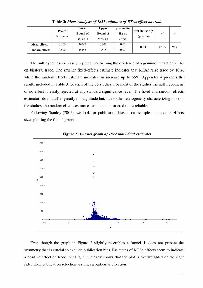
Table 3: Meta-Analysis of 1827 estimates of RTAs effect on trade

Pooled

Estimate

Lower

Bound of

95% CI

Upper

Bound of

95% CI

p-value for

H0: no

effect

test statistic Q

(p-value) H2 I2

Fixed-effects 0.100 0.097 0.101 0.00

Random-effects 0.500 0.482 0.515 0.00 0.000 47.65 98%

The null hypothesis is easily rejected, confirming the existence of a genuine impact of RTAs

on bilateral trade. The smaller fixed-effects estimate indicates that RTAs raise trade by 10%,

while the random effects estimate indicates an increase up to 65%. Appendix 4 presents the

results included in Table 3 for each of the 85 studies. For most of the studies the null hypothesis

of no effect is easily rejected at any standard significance level. The fixed and random effects

estimators do not differ greatly in magnitude but, due to the heterogeneity characterizing most of

the studies, the random effects estimates are to be considered more reliable.

Following Stanley (2005), we look for publication bias in our sample of disparate effects

sizes plotting the funnel graph.

Figure 2: Funnel graph of 1827 individual estimates

0

50

100

150

200

250

300

350

400

450

-10 -5 0 5 10 15

γγγγ

1/S

e

Even though the graph in Figure 2 slightly resembles a funnel, it does not present the

symmetry that is crucial to exclude publication bias. Estimates of RTAs effects seem to indicate

a positive effect on trade, but Figure 2 clearly shows that the plot is overweighted on the right

side. Then publication selection assumes a particular direction.

18

The six different estimates with the smallest standard errors do not differ significantly from each

other. The average of the top six points on the graph, that is the estimates associated with the

smallest standard errors, is equal to 0.04, implying a 4.1% increase in trade. Consequently, if

research reporting was unbiased, estimates should vary randomly and symmetrically around the

value 0.04, whereas the simple average of all 1827 estimates is 0.59, implying a 80% increase in

trade.

Table 4 reports the result of the MRA tests. Robust ordinary least squares estimation is used

and standard errors are recorded in parenthesis. Both tests confirm the presence of publication

bias and the existence of a positive impact. The estimate of β0 significantly different from 0

confirms the apparent asymmetry of the funnel graph; while the β1 estimate different from 0 and

a positive value for the α1 estimate, both statistically significant, provide evidence of a genuine

empirical effect.

Table 4: MRA tests of Effect and Publication Bias

Dependent Variables Variables

1: t 2:ln│t│

β0: intercept

3.53*

(0.16)

β1: 1/Se 0.03*

(0.01)

-

α1: Ln(n) - 0.25*

(0.02)

Obs 1827 1642

R-squared 0.01 0.14

S.E. of regression 6.18 1.18

Column 2: studies not reporting the number of observations are excluded

Standard errors are reported in parenthesis – *: significant at 1 percent.

After adding all of the explanatory variables discussed in the previous section, we dropped

the insignificant variables, one at a time, to yield the results for equation (16) presented in Table

5. The two columns 1 and 2 present the estimated coefficients (the standard errors adjusted for

85 studies/clusters are reported in parentheses) with and without the introduction of a fixed effect

for each type of agreement. Results show a significant general RTA effect on trade exceeding

11%. Comparing the two columns it appears that the results are by far and large robust.

The use of the log of average bilateral trade flows rather than the average of the logs of the

trade flows leads to significantly higher estimates of the RTAs effect. This result confirms and

provides a quantitative assessment of the silver medal mistake pointed out by Baldwin (see

19

section 4.1): the confusion between the log of the average and the average of the logs tends to

inflate the gravity estimates by 3 standard errors.

The time effects dummy is equal to “1” when time fixed effects are included in the

regression: this should control for the global trends existing in the data. In particular, time

dummies are expected to offset the bronze medal error implied by the mistaken deflation

procedure. The negative sign associated with this variable shows that uncorrected studies tend to

overestimate the RTAs impact on trade.

The country effect dummy is equal to “1” when the original studies use dummies to

characterize trade flows involving a particular country. Since this dummy is used to correct for

the “gold medal” mistake pointed out by Baldwin and Taglioni, the positive coefficient suggests

that the omitted variable bias leads to a serious underestimation of the RTAs trade impact.

Regarding the typologies of data used, we introduce 2 dummies with self-explanatory names:

cross-section and pooled.11 Results are negative for both variables confirming that cross-

sectional and pooled regression models may be affected by the exclusion or mismeasurement of

trading pair–specific variables (Baldwin, 2006). More specifically, our results support the claim

by Baier and Bergstrand (2005) that cross-section estimates are downward biased due to the

endogeneity problem.

As far as the estimation methods are concerned, the dummy ols equal to “1” if estimates are

obtained through simple OLS and “0” whether estimates are obtained with other approaches(i.e.,

instrumental variables, Hausman-Taylor, etc.). We find a positive and significant coefficient for

the ols dummy. As it was mentioned in the previous section, the OLS-estimator may yield biased

and inconsistent estimates due to omitted variables and selection bias. Trade between any pair of

countries is likely to be influenced by certain unobserved individual effects, if the unobserved

effects are correlated with the explanatory variables, coefficients of the latter may be higher

because they incorporate these unobserved effects. On the other hand, the dummy random effects

is equal to “1” when a panel model is estimated through a random effects approach. If we

believe, following Baier and Bergstrand (2005), that there unobserved time-invariant bilateral

variables influencing simultaneously the presence of a RTA and the volume of trade, the positive

coefficient of this dummy provides an estimate of the upward bias deriving from the assumption

of zero correlation between unobservables and RTAs.

Coming to the variables related to each study characteristics, we find a negative and highly

significant coefficient for the agreement dummy taking the value “1” if the original paper used a

variable for each type of agreement. Studies focusing on specific RTAs, then, tend to estimate

11 To avoid collinearity problems we do not include an additional dummy variable for panel studies.

20

much lower impacts on trade: apparently, the estimation problems do not cancel out when all the

RTAs are lumped together, rather they make the overestimation bias even larger.

The negative coefficient found for the dummy published may seem at odds with the picture

provided by the funnel graph. However, the negative bias of the published results may be a good

news, suggesting that editors do a pretty good job in excluding the highest (and possibly less

realistic) results. On the other hand, the dummy interested is strongly positive, hinting to the

existence of a “psychological bias”, since authors primarily interested in estimating the RTA

effect tend to report larger results.

As it was mentioned in the previous section, we handle the extreme values in the sample

adding a dummy called outliers. The estimated coefficient of this variable is clearly positive,

since most outliers indicate a positive and very high effect size of RTAs. In any case, the

removal of this dummy does not significantly affect the results.

Finally, we find significant and negative coefficients associated with the dummies for period

ranges (except for the 1970s). The effect size is much smaller before 1970, while the most recent

studies seem to get higher estimates. Such a result is consistent with the often noted evolution

from ‘shallow’ to ‘deep’ regional integration agreements, where the latter reduce trade costs

through behind-the-border reforms.

21

Table 5: Multivariate Meta-Regression Analysis (MRA) of Common RTAs Effects

Variables Coefficient

( Robust with Cluster Standard Errors)

Coefficient

( Robust with Cluster Standard Errors)

Intercept 3.27 (0.43) *** 2.73 (0.46) ***

1/Sei 0.11 (0.05) ** 0.11 (0.06)**

Log of average trade 0.13 (0.06) ** 0.15 (0.06)***

Time effects -0.14 (0.06) ** -0.14 (0.07)**

Country effects 0.35 (0.10) *** 0.36 (0.11)***

Random effects 0.14 (0.08) * 0.17 (0.08)**

Cross-section -0.21 (0.04) *** -0.21 (0.07) ***

Pooled -0.19 (0.04) *** -0.19 (0.05) ***

Ols 0.21 (0.04) *** 0.24 (0.05) ***

Agreement -0.10 (0.05) ** -

Interested 0.31 (0.07) *** 0.30 (0.07) ***

Published -0.10 (0.04) *** -0.15 (0.05) ***

Outliers 3.03 (0.26) *** 2.53 (0.60) ***

Before 1970 -0.35 (0.12) *** -0.29 (0.14) **

1970s 0.04 (0.22) 0.11 (0.24)

1980s -0.22 (0.09) *** -0.16 (0.09) *

After 1990 -0.20 (0.05) *** -0.17 (0.06) ***

Afta - 0.09 (0.19)

Aifta - -0.17 (0.06) ***

Anzcer - 0.24 (0.41)

Bfta - 1.90 (0.18) ***

Cacm - -0.04 (0.14)

Can - 0.36 (0.15) ***

Caricom - -0.06 (0.10)

Cefta - 0.12 (0.26)

Ciscu - 1.57 (0.19)***

Custa - -0.69 (0.07) ***

Efta - -0.12 (0.08)

Eu - -0.09 (0.05) *

Lafta - 0.69 (0.08) ***

Laia - -0.12 (0.09)

Mercosur - 0.12 (0.09)

Nafta - 0.12 (0.30)

Us-Chile - -0.67 (0.10)***

Us-Israel - 0.26 (0.08) ***

Obs

No of Clusters

R-squared

Prob > F

S.E. of regression

1827

85

0.25

0.00

5.40

1827

85

0.34

0.00

5.10

***:significant at 1 percent; **: significant at 5 percent; *: significant at 10 percent; All moderator variables are divided by Sei

22

- Focus on single RTAs.

46 studies out of 85 estimate the RTAs impact on trade introducing different dummies for

each trade agreement, yielding 1338 estimates. Table 6 summarizes the main results obtained for

each RTA.

Table 6: Descriptive statistics of estimates of single RTAs

Variable: γ Obs Mean Std. Dev. Min Max

RTAs 489 0.62 0.65 -3.97 4.83

Afta 41 0.81 0.69 -0.07 2.35

Aifta 10 0.06 0.04 0.00 0.10

Anzcer 15 0.87 1.10 -0.16 3.98

Bfta 24 2.96 0.43 2.37 3.77

Cacm 37 1.19 1.02 0.01 4.40

Can 13 1.34 0.55 0.12 2.22

Caricom 37 2.02 1.79 -0.35 5.23

Cefta 57 0.41 0.36 -0.51 1.52

Ciscu 6 2.66 0.60 1.98 3.37

Custa 63 -0.23 0.64 -1.89 2.26

Efta 343 0.23 0.50 -1.38 2.17

Eu 524 0.52 1.47 -9.01 15.41

Lafta 5 0.98 0.92 0.30 2.57

Laia 9 0.53 0.12 0.39 0.82

Mercosur 47 0.72 0.73 0.12 4.35

Nafta 90 0.90 1.06 -1.47 3.89

Us-Chile 5 0.27 0.66 -0.30 1.42

Us-Israel 12 0.82 0.75 -0.08 2.41

The largest number of observations refers to EU, one of the oldest and most studied case of

economic integration. Manifestly, the range between minimum and maximum estimates are very

large for the most of agreements, showing the large variety of estimates provided in the

literature.

Table 7 presents the results of the MA for the RTAs for which estimates are available. The tests

show that random effects estimates would be the most appropriate in most of the cases. Only 4

out of the 18 agreements do not show significant differences between fixed and random effects

estimates (in bold in the table), and most of these cases are characterized by a fairly low number

of observations.

23

Table 7: Meta-Analysis of estimates of specific RTAs

RTA Pooled

Estimate

Variation in

Trade (%)

Lower Bound

of 95% CI

Upper Bound

of 95% CI

test Q

(p-value) H2 I2

No. of

Estimates

Fixed 0.67 95% 0.63 0.70 Afta

Random 0.79 120% 0.60 0.99 0.00 30.92 97% 41

Fixed 0.07 7% 0.05 0.08 Aifta

Random 0.07 7% 0.05 0.09 0.18 1.40 29% 10

Fixed 0.73 107% 0.67 0.78 Anzcer

Random 0.88 142% 0.22 1.55 0.00 117.93 99% 15

Fixed 3.03 1972% 2.92 3.14 Bfta

Random 3.06 2026% 2.91 3.21 0.04 1.57 36% 24

Fixed 0.34 40% 0.31 0.37 Cacm

Random 1.03 179% 0.83 1.23 0.00 30.51 97% 37

Fixed 1.10 200% 1.00 1.19 Can

Random 1.23 242% 0.97 1.49 0.00 5.78 83% 13

Fixed 0.29 34% 0.26 0.32 Caricom

Random 1.69 440% 1.42 1.96 0.00 53.91 98% 37

Fixed 0.26 30% 0.24 0.28 Cefta

Random 0.40 49% 0.30 0.50 0.00 13.95 93% 57

Fixed 2.94 1795% 2.69 3.19 Ciscu

Random 2.82 1581% 2.38 3.26 0.02 2.61 62% 6

Fixed -0.34 -29% -0.36 -0.32 Custa

Random -0.25 -22% -0.36 -0.14 0.00 2.13 53% 63

Fixed 0.05 6% 0.05 0.06 Efta

Random 0.24 27% 0.21 0.28 0.00 18.92 95% 343

Fixed 0.05 6% 0.05 0.06 Eu

Random 0.35 41% 0.32 0.37 0.00 59.27 98% 524

Fixed 1.14 213% 1.07 1.21 Lafta

Random 0.98 168% 0.16 1.81 0.00 133.70 99% 5

Fixed 0.52 68% 0.47 0.57 Laia

Random 0.52 69% 0.45 0.60 0.13 1.58 37% 9

Fixed 0.37 45% 0.35 0.39 Mercosur

Random 0.64 90% 0.55 0.74 0.00 16.36 94% 47

Fixed 0.80 123% 0.76 0.85 Nafta

Random 0.84 131% 0.64 1.04 0.00 17.98 94% 90

Fixed 0.13 14% -0.04 0.30 Us-Chile

Random 0.27 31% -0.31 0.85 0.00 9.94 90% 5

Fixed 0.80 122% 0.72 0.87 Us-Israel

Random 0.84 131% 0.47 1.21 0.00 19.87 95% 12

The largest effect is registered for the Baltics-RTA (BFTA): the fixed effects estimate

suggests an increase in trade around 2000%! Other agreements presenting exceedingly high

estimates are the CISCU (1581%) and the Caribbean Community (400%) (Figure 3) .

24

Figure 3: Meta-Analysis of estimates of specific RTAs

-100% 100% 300% 500% 700% 900% 1100% 1300% 1500% 1700% 1900% 2100%

Afta

Aifta

Anzcer

Bfta

Cacm

CanCaric

om

Cefta

Ciscu

Custa

Efta

Eu

Lafta

LaiaMercosur

NaftaUs-C

hileUs-Is

rael

Random Effects

Fixed Effects

Looking at the most widely studied agreements – EU, EFTA and NAFTA –, the largest

impact is for NAFTA (131%), while the European agreements register much lower, but possibly

more realistic values: 27% in the case of EFTA, 41% for the EU. It is also worth noting that

custom unions – EU, CARICOM, MERCOSUR, CACM, CISCU – does not seem to consistently

outperform the free trade areas in terms of trade impact. Indeed, in the meta-analysis regression

the coefficient of the CU variable was never significant.

4.3 Probit Significance Equation

In our dataset of 1827 effect sizes, 1134 are significantly different from zero at the level of

5%, and 1048 of these estimates are positive. This is the sample used in the probit estimate

(equation 17). The results in terms of the marginal effects at the sample means are shown in

Table 8. The value at the mean of the linear combination of the explanatory variables (Z) is 0.22,

while the marginal probability of finding a positive and significant impact on trade is 0.4.

Since we use the same set of variables presented in section 4.1, we can compare these results

with those presented in table 5. We single out 3 groups of variables: significant variables in both

cases with the same sign; significant variables in both cases with opposite signs; significant

variables in the probit regression that were dropped from the MRA.

In the first group we find the dummies for the different decades, the log of the average, the

analysis of specific RTAs , the presence or not of country effects, the use of a random effects

model in panel estimations, and the primary focus of the analysis. In these cases, then, the probit

25

estimates are largely consistent with the evidence provided by the MRA. Firstly, the assessments

of older agreements (or first stages of implementation) are less likely to detect a positive impact

on trade: using data before 1970, for instance, reduces the probability by almost 40 percent. By

the same token, the use of data on specific agreements reduces the probability of estimating a

positive impact on trade by 20 percent, as it could have been expected given that the estimates

provided by these studies are generally lower. On the contrary, confusion between the log of the

average and the average of the logs (the “silver medal mistake”), omitted variables bias (country

effects), panel estimates through random effects, and interest in estimating the RTA impact

substantially raise the probability to find a positive and significant effect: a likely consequence of

the overestimation highlighted by the MRA.

In the second group, we find that the dummies for the time effects, the data used, the

estimation method, and the publication bias. In these cases, the probit estimates indicate a lower

(higher) probability to get significant estimates, even if the effect sizes show an upward

(downward) bias. Accordingly, studies offsetting the “bronze medal error” (time effects) or

formally published are more likely to find significant results, even if their estimates tend to be

smaller; while the positive sign associated with the cross-section and pooled dummies suggests

that the downward bias indicated by the MRA is mostly due to non significant estimates. On the

other hand, the estimation problems related to the OLS decrease the probability of getting

significant results, even if these estimates tend to be inflated.

In the third group, we find the methodological dummies related to studies using dynamic

techniques (dynamic) or dealing with the multilateral trade resistance term (Anderson-van

Wincoop), and the selection bias and the presence of zero trade flows (Heckman, Tobit, Poisson).

In these cases, even if there is not an evidence of a significant impact on the effect size when we

use the largest sample, there seems to be a negative sign associated with the significant

estimates. Accordingly, the use of more sophisticated estimation methods increases the

probability of getting lower, though, still positive estimates of the RTAs impact on trade.

26

Table 8: Probit Analysis

Probit Estimation Mean β Mean* β f(Z) f(Z)

Before 1970 0.06 -0.92*** -0.06 0.40 -0.37

1970s 0.07 -0.57*** -0.04 0.40 -0.23

1980s 0.20 -0.82*** -0.16 0.40 -0.33

After 1990 0.43 -0.25*** -0.11 0.40 -0.10

Log of average trade 0.20 0.29** 0.06 0.40 0.12

Anderson-van Wincoop 0.11 0.59*** 0.07 0.40 0.23

Time effects 0.12 0.27** 0.03 0.40 0.11

Country effects 0.04 0.45** 0.02 0.40 0.18

Random effects 0.04 0.53*** 0.02 0.40 0.21

Pooled 0.31 0.54*** 0.17 0.40 0.22

Cross-section 0.44 0.42*** 0.18 0.40 0.17

Ols 0.71 -0.44*** -0.31 0.40 -0.18

Heckman 0.02 -0.44* -0.01 0.40 -0.18

Tobit 0.06 -0.83*** -0.05 0.40 -0.33

Poisson 0.05 -0.68*** -0.04 0.40 -0.27

Dynamic 0.03 -0.54*** -0.02 0.40 -0.21

Agreement 0.73 -0.50*** -0.37 0.40 -0.20

Published 0.40 0.20*** 0.08 0.40 0.08

Interested 0.39 0.45*** 0.18 0.40 0.18

Intercept 1.00 0.57*** 0.57 0.40 0.23

Total 0.22

No. of Obs 1048

Wald χ2(19)

(p-value)

340

(0.000)

Pseudo R2 0.14

*: significant at 5%; **: significant at 1%.

5. Conclusion.

RTAs have been widely studied, and the interest on this type of trade liberalization is likely

to increase in the next future due to the crisis of the multilateral liberalization process. One way

to carry out a comparative study of the empirical results is to simply tabulate authors, country,

methodology, and results. However, for policy analysis and a better understanding of the

consequences of RTAs, it is useful to complement broad qualitative conclusions with a more precise

quantitative research synthesis. This is the purpose of the present paper with respect to one core

issue: the impact of these agreement on member countries’ bilateral trade flows. In particular, we

decided to overcome the main limitations of qualitative reviews, summarizing statistically the whole

body of work through meta-regression analysis.

27

In this paper, we have investigated the result of previous studies analysing the effect of

RTAs: the estimated effect varies widely from study to study and sometimes even within the

same study. From the methodological point of view, this suggests the opportunity to retain all the

available observations in most of our statistical analysis, though considering estimates from the

same study as possibly correlated observations. Accordingly, by means of meta-analysis

techniques, we statistically summarized 1827 estimates collected from a set of 85 studies.

All combined estimates imply a substantial increase in trade, but they vary a lot depending

on the estimation method. In particular, the ‘random-effects’ estimate entails an increase of 65%.

The more modest ‘fixed-effects’ estimate (10%) cannot be trusted because its basis is

undermined by obvious heterogeneity in this literature. However, there is also strong statistical

evidence of publication selection, favoring the reporting of significantly positive trade effects:

such publication bias causes all simple combined estimates of trade effects, whether fixed- or

random-effects, to be exaggerated.

Our analysis also provides a range of additional results helping to explain the wide variation in

reported estimates. In this respect, meta-analysis statistical techniques are something more than

mere weighted averages of all point estimates. Even if we do not dare to assign “weights” (or

“medals”) according to which of the studies we deem as good or bad, we do provide a

quantitative assessment of the coonsequences due to the publication selection or possibly

questionable methodological choices. For example, estimates obtained from cross and pooled

data are more likely to find a positive and significant impact, though they report smaller values.

The same example is possible for fixed and random effect estimators. On the other hand, studies

reporting OLS estimates are less likely to get (statistically speaking) “good results” and provide

results that may be upward biased due to misspecifications and omitted variables. Several studies

lump different trade agreements together: this has a negative impact on the likelihood of finding

significant results, and lead to an underestimation of the impact on trade. Conversely, published

papers and studies mainly interested in studying the RTAs’ impact are more likely to report

significant results that tend to be overestimated.

After filtering out the publication selection and other biases, the meta-analysis confirms a

robust, positive RTA effect, equivalent to an increase in trade exceeding 11%. The estimates

tend to get larger in recent years, and this could be a consequence of the evolution from

‘shallow’ to ‘deep’ trade agreements. Looking at fixed effects for type of trade agreement, we

find evidence of a differentiated impact on trade, the majority of coefficients are positive and

strongly significant, although they are lower than results obtained by single MA for specific

RTAs. Indeed, in many cases the MA estimate of the impact on trade for type of agreement

largely exceeds the estimate for all the agreements combined.

28

The meta-analysis of the trade effects of RTAs provide a combined estimate more plausible

than some extreme values reported in the literature. Moreover, our results shed some light on the

role played by some research characteristics in explaining the variation in reported estimates.

However, our findings should still be considered as provisional, since there remains excess

unexplained variation in our meta-regression models.

29

References

Adam A., Kosma T. S., McHugh J. (2003), Trade-Liberalization Strategies: What Could

Southeastern Europe Learn from the CEFTA and BFTA?, IMF Working Paper, WP/03/239. Aiello F., Agostino M.R., Cardanone P. (2006), Reconsidering the Impact of Trade

Preferences in Gravity Models. Does Aggregation Matter?, University of Calabria, unpublished. Aikeen (1973), The effect of the EEC and EFTA on European trade: A temporal Cross-

section Analysis, The America Economic Review, vol. 63, no.5. Anderson J.E., van Wincoop E. (2003), Gravity With Gravitas: A Solution to the Border

Puzzle, American Economic Review, 93(1): 170-192. Ashenfelter O., Harmon C., Oosterbeek H. (1999), A review of estimates of the

schooling/earnings relationship, with tests for publication bias, Labour Economics, No. 6, pp. 453-470.

Baier, Bergstrand (2005), Do Free Trade Agreements Actually Increase Members’

International Trade? Federal Reserve Bank of Atlanta, WP 2005-3. Baldwin R., Taglioni D. (2006), Gravity for dummies and dummies for gravity equations,

NBER Workin Paper No. 12516. Baldwin R.E. (1994), Towards an Integrated Europe, London: Centre for Economic Policy

Research. Baldwin R.E. (2006), The Euro’s Trade Effects, European Central Bank Working Paper

Series, 594. Baxter M., Kouparitsas M. A . (2006), What determines bilateral trade flows?, NBER

Working Paper No. 12188. Bayoumi, Eichengreen (1995), Is regionalism simply a diversion? Evidence from the

evolution of the EC and EFTA, NBER WP 5283. Bergstrand J. (1985), The gravity equation in international trade: some microeconomic

foundation and empirical evidence, The Review of Economics and Statistics 67, 474– 481. Bergstrand J. H. (1989), The Generalized Gravity Equation, Monopolistic Competition, and

the Factor Proportions Theory in International Trade, Review of Economic and Statistics 71: 143-53.

Bijmolt, T.H.A. and R.G.M. Pieters, 2001, Meta-Analysis in Marketing when Studies

Contain Multiple Measurements”, Marketing Letters, 12(2): 157-169. Blomqvist H.C. (2004), Explaining Trade Flows of Singapore, Asian Economic Journal, Vol.

18, No. 1. Brada J. C., Mendez J. A. (1985 ), Economic integration among developed, developimg and

centrally planned economics: a comparative analysis, Review of Economics and Statistics, 67, pp. 549-56.

Breuss F., Egger P. (1999), How reliable are estimations of East-West Trade potentials

based on Cross-Section Gravity Analyses?, Empirica, 26, pp. 81-94. Broto C., Ruiz J., Vilarrubia1 J. (2006), Firm heterogeneity, and selection bias: estimating

trade potentials in the Euromed region, Bank of Spain, unpublished. Bun M. J., Klassen F. J.G.M. (2002), Has the Euro increase Trade?, Tibergen Institute

Discussion Paper 2002-108/2. Bun M. J., Klassen F. J.G.M. (2006), The Euro Effect on Trade is not as Large as Commonly

Thought, Forthcoming in the Oxford Bulletin of Economics and Statistics. Card D., Krueger A.B. (1995), Time-Series Minimum-Wage Studies: a Meta-analysis, The

American Economic Review, 85(2): 238-243. Carrère C. (2006), Revisiting the Effects of Regional Trading Agreements on Trade Flows

with Proper Specification of the Gravity Model, European Economic Review, 50, pp. 223-247. Cernat L. (2001), Assensing regional trade arrangements: are south-south RTAs more trade

diverting?, Policy Issues in International Trade and Commodities Study Series No. 16, United Nations Conference on Trade and Development.

30

Cheng I-H., Tsai Y-Y. (2005), Estimating the Staged Effects of Regional Economic

Integration on Trade Volumes, Department of Applied Economics, Taiwan, unpublished. Cheng I-H., Wall H. J. (2004), Controlling for Heterogeneity in Gravity Models of Trade and

Integration, Working Paper Series 1999-010E, The Federal Reserve Bank of St. Louis. Clarete R., Edmonds C., Wallack J.S. (2003), Asian regionalism and its effects on trade in

the 1980s and 1990s, Journal of Asian Economics 14 91–129 Colin J. R. (2005), Issues in Meta-Regression Analysis: an overview, Journal of Economic

Surveys 19: 295-298 De Benedictis L., De Santis R.,Vicarelli C. (2005), Hub-and Spoke or else? Free trade

agreements in the enlarged EU. A gravity model estimate, European Network of Economic Policy Research Istitutes, Working Paper No. 37.

Disdier A. C., Head K. (2004), The Puzzling Persistence of the Distance Effect on Bilateral

Trade, Centro Studi Luca D’Agliano, Development Studies Working Papers No. 186. Eaton J., Kortum S. (1997), Technology and Bilateral Trade, NBER Working Paper No.

6253. Egger P. (2005), Alternative Techniques for Estimation of Cross-Section Gravity Models,

Review of International Economics, 13(5), pp. 881–891. Eichengreen, B., Irwin, D., 1996. The Role of History in Bilateral Trade Flows. NBER

Working Paper No. 5565. Elliot R. J., Ikemoto K. (2004), AFTA and the Asian Crisis: Help or Hindrance to ASEAN

intra-regional trade?, Asian Economic Journal, vol. 18(1):1-10. Endoh M. (2000), The transition of post-war Asia-Pacific trade relations, Journal of Asian

Economics 10, pp. 571–589. Faruquee H. (2004), Measuring the Trade Effects of EMU, IMF Working Paper WP/04/154. Fazio G., MacDonald R., Mélitz J. (2005), Trade costs, trade balances and current accounts:

an application of gravity to multilateral trade, CEPR Discussion Paper No. 5137. Feenstra R. C. (1998), Integration of Trade and Disintegration of Production in the Global

Economy, Journal of Economic Perspectives, 12, 31-50. Feenstra, Markusen, Rose (2001), Using the gravity equation to differentiate among

alternative theories of trade, Canadian Journal of Economics, vol. 34, no.2. Fidrmuc J., Fidrmuc J. (2003), Disintegration and trade, Review of International Economics

11(5): 811–829. Fisher R.A. (1932), Statistical Methods for Research Workers, 4th edn, Oliver andBoyd,

London. Florax, R., de Groot H., de Mooij R. (2002), Meta-analysis in policy-oriented economic

research, CPB, Report # 1: 21-24. Frankel J. A., Rose A. K. (2000), An estimate of the effect of currency unions on trade and

output, CEPR, Discussion Paper No. 2631. Frankel J. A., Stein E., Wei S-J. (1995), Trading blocs and the Americas: The natural, the

unnatural, and the super-natural, Journal of Development Economics Vol. 47, pp. 61-95 Frankel J. A., Stein E., Wei S-J. (1997), Regional Trading Blocs. Institute for International

Economics. Frankel J. A., Wei (1995), Open regionalism in a world of continental trade blocs, NBER

Working Paper No.5272. Frankel J. A., Wei S-J. (1997), ASEAN in a Regional Perspective, in J. Hicklin, D. Robinson

and A. Singh, eds., Macroeconomic Issues Facing ASEAN Countries. Washington, DC: International Monetary Fund.

Fratianni M., Kang H. (2006), Heterogeneous distance–elasticities in trade gravity models, Economics Letters 90, pp. 68–71

Freund C. L., Weinhold D. (2004), The effect of the Internet on international trade, Journal of International Economics 62, pp. 171– 189

31

Gaulier G., Jean S., Ünal-Kesenci D. (2004), Regionalism and the Regionalisation of

International Trade, CEPII, Working Paper No 2004-16 Ghosh, Yamarik, (2004), Are regional trading arrangements trade creating? An application

of extreme bounds analysis, Journal of International Economics, 63. Glass G.V., McGaw B., Lee Smith M. (1981), Meta-analysis in Social Research, Sage

Publications, Beverly Hills. Glick R., Rose A. K. (2002), Does a currency union affect trade? The time series evidence,

European Economic Review 46(6): 1125–1151. Greenaway D., Milner C. (2002), Regionalism and Gravity, Scottish Journal of Political

Economy, Vol. 49, No. 5 Grünfeld L. A., Moxnes A. (2003), The Intangible Globalization. Explaining the Patterns of

International Trade in Services, NUPI Paper No. 657. Hassan (2001), Is SAARC a viable economic block? Evidence from gravity model, Journal of

Asian Economics, 12. Heckman J. J. (1997), Instrumental Variables: A Study of Implicit Behavioral Assumptions

Used in Making Program Evaluations, Journal of Human Resources 32, No. 3, pp. 441-462. Hejazi ., Safarian A.E. (2005), NAFTA effects and the level of development, Journal of

Business Research 58, pp. 1741– 1749 Higgins J. P. T., Thompson S. G. (2002), Quantifying heterogeneity in a meta-analysis,

Statistics in Medicine 21: 1539–1558. Jakab Z. M., Kovacs M. A., Oszlay A. (2001), How Far Has Trade Integration Advanced?:

An Analysis of the Actual and Potential Trade of Three Central and Eastern European

Countries, Journal of Comparative Economics 29, pp. 276–292 Jarrell S. B., Stanley T. D. (1990), A meta-analysis of the union wage gap, Industrial and

Labour Relations Review 44, pp. 54–67 Jayasinghe, Sarker (2004), Effects of Regional Trade Agreements on Trade in Agrifood

Products: Evidence from Gravity Modeling Using Disaggregated Data, Center for Agricultural and Rural Development Iowa State University, Working Paper 04-WP 374.

Jeppesen, T., List J.A., Folmer H., (2002), Environmental Regulations and New Plant

Location Decisions: Evidence from a Meta-Analysis, Journal of Regional Science, 42(1): 19-49. Katayama H., Melatos M. (2006), Currency Unions Cannot Defy Gravity – Mind the Curves

and (Slippery) Slopes, University of Sydney, unpublished Kein N. T., Hashimoto Y. (2005), Economic analisys of ASEAN Free Trade Area; by a

country panel data, Discussion Papers in Economics and Business, No. 05-12. Kenen P. B. (2002), Currency unions and trade: Variations on themes by Rose and Persson,

RBNZ DP/2002/08. Kimura F., Lee H-H. (2004), The Gravity Equation in International trade in Services,

Kangwon National University, Korea, unpublished. Klein M. W. (2005), Dollarization and trade, Journal of International Money and Finance,

24, pp. 935-943. Knell M., Stix, H. (2005), The income elasticity of money demand: a meta-analysis of

empirical results, Journal of Economic Surveys 19, pp. 513–533. Krueger A. (1999), Trade creation and trade diversion under Nafta, NBER WP.4729. Lee J-W., Park I. (2005), Free Trade Areas in East Asia: Discriminatory or Non-

discriminatory?, The World Economy, Vol. 28, No.1, pp 21-48. Lee J-W., Park I., Shin K. (2004), Proliferating Regional Trade Arrangements: Why and

Whither?, Korea University, unpublished. Lennon C. (2006), Trade in Services and Trade in Goods: Differences and

Complementarities, University of Paris 1 and Paris-Jourdan Sciences Economiques, unpublished Levine R., Renelt D. (1992), A Sensitivity Analysis of Cross-Country Growth Regressions,

American Economic Review, 82 (4), pp. 942–963.

32

Longhi S., Nijkamp P., Poot J. (2005), A meta-analytic assessment of the effect of

immigration on wages, Journal of Economic Surveys, Vol. 19, pp. 451–478. Longhi S., Nijkamp P., Poot J. (2006), The fallancy of “Job Robbing”, Tinbergen Istitute

Discussion Paper, TI 2006-050/3. Màrquez-Ramos L., Martìnez-Zarzoso I., Suàrez-Burguet C. (2006), The role of distance in

gravity regressions: is there really a missing globalisation puzzle?, unpublished Martìnez-Galàn E., Fontoura M. P., Proenca I. (2005), Trade Potential in an Enlarged

European Union: a recent approach, ISEG, unpublished. Martinez-Zarsoso I., Nowak-Lehman F. (2003), Augmented Gravity Model: An Empirical

Application to Mercosur-European Union Trade Flows, Journal of Applied Economics, Vol. 6, No. 2, pp. 291-316.

Martìnez-Zarzoso I., Horsewood N. (2005), Regional trading agreements: Dynamic panel

data evidence from the gravity model, unpublished. Mayer T, Zignago S. (2005), Market Access in Global and Regional Trade, CEPII Working

Paper No. 2005-02. Meade J. (1955), The theory of customs unions (North-Holland, Amsterdam). Melitz J. (2001), Geography, trade and currency union, CEPR Discussion Paper, No. 2987. Melitz J. (2002), Language and foreign trade, University of Strathclyde working paper,

unpublished. Micco A., Stein E., Ordon˜ ez G. (2003), The currency union effect on trade: Early evidence

from EMU, Economic Policy, Vol. 37, pp. 316–356. Nijkamp P., Poot J. (2005), The last word on the wage curve?, Journal of Economic Surveys,

Vol.19, pp. 421–450. Nitsch V. (2002), Honey, I shrunk the currency union effect on trade, World Economy, Vol.

25, No. 4, pp. 457–474. Paiva C (2005), Assessing Protectionism and Subsidies in Agriculture: A gravity Approach,

IMF Working Paper, WP/05/21. Pakko M. R., Wall H. J. (2001), Reconsidering the trade-creating effects of a currency union,

FRB St. Louis Review, Vol. 83, No. 5, pp. 37–45. Papazoglou C, Pentecost E. J., Marques H. (2006), A Gravity Model Forecast of the

Potential Trade Effects of EU Enlargement: Lessons from 2004 and Path-dependency in

Integration, The World Economy. Rauch J. (1996), Networks versus markets in International Trade, NBER Working Paper No.

5617. Rauch J., Trindade V. (1999), Ethnic Chinese Networks in International Trade, NBER

Working Paper No. 7189. Rose A. K. (2000), Currency Unions. Their dramatic effect on international trade, Economic

Policy, April. Rose A. K. (2001), Currency unions and trade: The effect is large, Economic Policy, Vol.

33, pp. 449–461. Rose A. K. (2004), Do We Really Know that the WTO Increases Trade?, American

Economic Review, Vol. 94(1). Rose A. K. (2005a), Does the WTO Make Trade More Stable?, Open Economics Review,

No. 16. Rose A. K. (2005b), One reason countries pay their debts: renegotiation and international

trade, Journal of Development Economics, Vol. 77, pp. 189– 206 Rose A. K., Engel C. (2002), Currency unions and international integration, Journal of

Money, Credit, and Banking, Vol. 34, No. 4, pp. 1067–1089. Rose A. K., Stanley T. D. (2005), Meta-analysis of the effect of common currencies on

international trade, Journal of Economic Surveys, Vol. 19, pp. 347–366. Rose A. K., van Wincoop E. (2001), National money as a barrier to trade: The real case for

monetary union, American Economic Review, Vol. 91, No. 2, pp. 386–390.

33

Saiki A. (2005), Asymmetric Effect of Currency Union for Developing Countries, Open Economies No. 16.

Sanso M., Cuairan R., Sanz F. (1993), Bilateral Trade Flows, the Gravity Equation, and

Functional Form, The Review of Economics and Statistics, Vol. 75, No. 2, pp. 266-275 Sapir A. (2001), Domino effects in Western European regional trade, 1960–1992, European

Journal of Political Economy, Vol. 17, pp. 377-388 Siliverstovs B., Schumacher D. (2006), To log or not to log, or How to estimate a gravity

model?, DIW Berlin, unpublished Silva J. S., Tenreyro S. (2003), Gravity-Defying Trade, unpublished. Silva J. S., Tenreyro S. (2005), The Log of Gravity, CEPR Discussion Paper No.5311. Sissoko A. A. (2004), Measuring Trade Intensity within the European Zone, unpublished. Soloaga, Winters (2001), Regionalism in the nineties: What effect on trade?, North American

Journal of Economics and Finance, Vol. 12, pp. 1-29 Stanley T. D. (2004), Meta-regression methods for detecting and estimating empirical effect

in the presence of publication selection, Center for Entrepreneurial Studies Discussion Paper 2004–2, Hendrix College.

Stanley T. D. (2005), Beyond publication bias, Journal of Economic Surveys, Vol. 19, pp. 309–346.

Stanley T. D., Jarrell S. B. (1989), Meta-regression analysis: a quantitative method of

literature surveys, Journal of Economic Surveys Vol. 3, pp. 54–67. Stanley T. D., Jarrell S. B. (1998), Gender wage discrimination bias? A meta-regression

analysis, Journal of Human Resources, Vol. 33, pp. 947–973. Stanley T. D., Jarrell S. B. (2005), Meta-regression analysis: a quantitative method of

literature surveys, Journal of Economic Surveys, Vol. 19, pp. 299–308. Stanley T.D. (2001), Wheat From Chaff: Meta-Analysis as Quantitative Literature Review,

Journal of Economic Perspectives, Vol. 15, pp. 131–150 StataCorp. (2005), Stata Statistical Software: Release 9. College Station, TX: Stata-Corp LP. Subramanian A., Wei S.-J. (2003), The WTO promotes trade, strongly but unevenly, NBER

Working Paper No.10024. Subramanian A., Wei S.-J. (2005), The WTO promotes trade, strongly but unevenly, CEPR

Discussion Paper No 5122. Sutton A.J., Abrams K.R., Jones D.R., Sheldon T.A., Song F. (2000), Methods for Meta-

Analysis in medical research, Chichester: John Wiley & Sons, 2000. Tang D. (2005), Effects of the Regional Trading Arrangements on Trade: Evidence from the

NAFTA, ANZCER and ASEAN Countries, 1989 – 2000, Journal of International Trade & Economic Development, Vol. 14, No. 2, pp. 241 – 265.

Tenreyro S. (2001), On the causes and consequences of currency unions, Harvard University, unpublished.

Thom R., Walsh B. (2002), The effect of a common currency on trade: Ireland before and

after the sterling link, European Economic Review, Vol.46, No. 6, pp. 1111–1124. van den Bergh J., Button K.J. (1997), Meta-analysis of Environmental Issues in Regional

Urban and Transport Economics, Urban Studies, 34(5-6), pp. 927-944. Verdeja L. (2005), EU’s Preferential Trade Agreements With Developing Countries

Revisited, unpublished. Viner J. (1950), The Customs Union Issue, Carnegie Endowment for International Peace,

New York. Walsh K. (2006), Trade in Services: Does Gravity Hold? A Gravity Model Approach to

Estimating Barriers to Services Trade, Trinity College, Dublin, unpublished. Weichselbaumer D., Winter-Ebmer R. (2005), A meta-analysis of the international gender

wage gap, Journal of Economic Surveys, Vol. 19, pp. 479–512. World Bank, (2005), Global Economic Prespectives 2005, Regional Trade Agreements:

Effects on Trade, Chapter 3.

34

Yeyati L. E. (2003), On the impact of a common currency on bilateral trade, Economics Letters Vol. 79, No. 1, pp. 125–129.

35

APPENDIX 1

Reciprocal Trade Agreements (in chronological order of date of entry into force) Trade Agreements Date

European Union (EU): Belgium-Luxembourg, France, Germany, Italy, Netherlands Denmark, Ireland, United Kingdom Greece Portugal, Spain Austria, Finland, Sweden Cyprus, Czech Rep., Estonia, Hungary, Latvia, Lithuania, Malta, Poland, Slovak Rep., Slovenia European Free Trade Association (EFTA): Switzerland, United Kingdom Norway, Portugal Sweden Denmark Finland Austria Latin American Free Trade Agreement/Latin American Integration

Agreement, (LAFTA/ LAIA): Argentina, Bolivia, Brazil, Chile, Ecuador, Mexico, Paraguay, Peru, Uruguay, Venezuela Central American Common Market (CACM): El Salvador, Guatemala, Honduras, Nicaragua, Costa Rica Anglo–Irish Free Trade Area Agreement (AIFTAA)

Caribbean Community (CARICOM): Jamaica, Trinidad and Tobago, Guyana Australia -New Zealand Closer Economic Relations (ANZCER)

US-Israel

US-Canada (CUFTA)

Central Europe Free Trade Agreement (CEFTA): Hungary, Poland, Romania Bulgaria Baltic FTA(BFTA): Estonia, Latvia, Lithuania Commonwealth of Independent States (CIS): Russia, Kazakhstan, Ukraine, and Belarus NAFTA:

Mercado Comun del Sur (Mercosur): Argentina, Brazil, Paraguay, Uruguay Association of Southeast Nations ASEAN (AFTA): Indonesia, Philippines, Singapore, Thailand US-Chile

1958 1973 1981 1986 1995 2004 1960 Until 1973 Until 1986 Until 1995 1973 1986-1995 1995

1961-1979, 1993 ineffective 1980-1990 reinitiated 1993 1961-1975, 1993 1965 1965

1968 1995 1983

1985

1989

1993

1997 1998 1993

1993

1995

1991 formed in 1991 and FTA in 1995 1998

2004

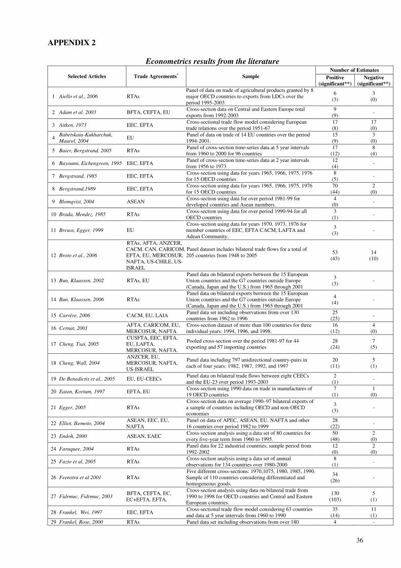
36

APPENDIX 2

Econometrics results from the literature Number of Estimates

Selected Articles Trade Agreements* Sample Positive

(significant**)

Negative

(significant**)

1 Aiello et al., 2006 RTAs Panel of data on trade of agricultural products granted by 8 major OECD countries to exports from LDCs over the period 1995-2003.

6 (3)

3 (0)

2 Adam et al. 2003 BFTA, CEFTA, EU Cross-section data on Central and Eastern Europe total exports from 1992-2003

9 (9)

-

3 Aitken, 1973 EEC, EFTA Cross-sectional trade flow model considering European trade relations over the period 1951-67

17 (8)

17 (0)

4 Babetskaia-Kukharchuk,

Maurel, 2004 EU

Panel of data on trade of 14 EU countries over the period 1994-2001.

15 (9)

3 (0)

5 Baier, Bergstrand, 2005 RTAs Panel of cross-section time-series data at 5 year intervals from 1960 to 2000 for 96 countries

17 (12)

8 (4)

6 Bayoumi, Eichengreen, 1995 EEC, EFTA Panel of cross-section time-series data at 2 year intervals from 1956 to 1973

12 (4)

-

7 Bergstrand, 1985 EEC, EFTA Cross-section using data for years 1965, 1966, 1975, 1976 for 15 OECD countries

8 (5)

-

8 Bergstrand,1989 EEC, EFTA Cross-section using data for years 1965, 1966, 1975, 1976 for 15 OECD countries

70 (44)

2 (0)

9 Blomqvist, 2004 ASEAN Cross-section using data for over period 1981-99 for developed countries and Asean members.

4 (0)

-

10 Brada, Mendez, 1985 RTAs Cross-section using data for over period 1990-94 for all OECD countries

3 (1)

-

11 Breuss, Egger, 1999 EU Cross-section using data for years 1970, 1973, 1976 for member countries of EEC, EFTA CACM, LAFTA and Adean Community.

3 (3)

-

12 Broto et al., 2006

RTAs, AFTA, ANZCER, CACM, CAN, CARICOM, EFTA, EU, MERCOSUR, NAFTA, US-CHILE, US-ISRAEL

Panel dataset includes bilateral trade flows for a total of 205 countries from 1948 to 2005

53 (43)

14 (10)

13 Bun, Klaassen, 2002 RTAs, EU Panel data on bilateral exports between the 15 European Union countries and the G7 countries outside Europe (Canada, Japan and the U.S.) from 1965 through 2001

3 (3)

-

14 Bun, Klaassen, 2006 RTAs Panel data on bilateral exports between the 15 European Union countries and the G7 countries outside Europe (Canada, Japan and the U.S.) from 1965 through 2001

4 (4)

-

15 Carrère, 2006 CACM, EU, LAIA Panel data set including observations from over 130 countries from 1962 to 1996

25 (25)

-

16 Cernat, 2001 AFTA, CARICOM, EU, MERCOSUR, NAFTA

Cross-section dataset of more than 100 countries for three individual years: 1994, 1996, and 1998.

16 (12)

4 (0)

17 Cheng, Tsai, 2005

CUSFTA, EEC, EFTA, EU, LAFTA, MERCOSUR, NAFTA.

Pooled cross-section over the period 1981-97 for 44 exporting and 57 importing countries

28 (24)

7 (5)

18 Cheng, Wall, 2004

ANZCER, EU, MERCOSUR, NAFTA, US-ISRAEL

Panel data including 797 unidirectional country-pairs in each of four years: 1982, 1987, 1992, and 1997

20 (11)

5 (1)

19 De Benedictis et al., 2005 EU, EU-CEECs Panel data on bilateral trade flows between eight CEECs and the EU-23 over period 1993-2003

2 (1)

-

20 Eaton, Kortum, 1997 EFTA, EU Cross-section using 1990 data on trade in manufactures of 19 OECD countries

7 (1)

1 (0)

21 Egger, 2005 RTAs Cross-section data on average 1990–97 bilateral exports of a sample of countries including OECD and non-OECD economies

3 (3)

-

22 Elliot, Ikemoto, 2004 ASEAN, EEC, EU, NAFTA

Panel on data of APEC, ASEAN, EU, NAFTA and other 16 countries over period 1982 to 1999

28 (22)

-

23 Endoh, 2000 ASEAN, EAEC Cross-section analysis using a data set of 80 countries for every five-year term from 1960 to 1995.

50 (48)

2 (0)

24 Faruquee, 2004 RTAs Panel data for 22 industrial countries, sample period from 1992-2002

12 (0)

2 (0)

25 Fazio et al, 2005 RTAs Cross-section analysis using a data set of annual observations for 134 countries over 1980-2000

8 (1)

-

26 Feenstra et al 2001 RTAs Five different cross-sections: 1970,1075, 1980, 1985, 1990. Sample of 110 countries considering differentiated and homogeneous goods.

34 (26)

-

27 Fidrmuc, Fidrmuc, 2003 BFTA, CEFTA, EC, EC+EFTA, EFTA,

Cross-section analysis using data on bilateral trade from 1990 to 1998 for OECD countries and Central and Eastern European countries.

130 (103)

5 (1)

28 Frankel, Wei, 1997 EEC, EFTA Cross-sectional trade flow model considering 63 countries and data at 5 year intervals from 1960 to 1990

35 (14)

11 (1)

29 Frankel, Rose, 2000 RTAs Panel data set including observations from over 180 4 -

37

countries at 5-year intervals from 1970 through 1995 (4)

30 Frankel, Stein, Wei, 1995 EEC, EFTA Cross-sectional trade flow model considering 63 countries and data at 5 year intervals from 1965 to 1990

25 (10)

11 (0)

31 Frankel, Stein, Wei, 1997 EC Cross-sectional trade flow model considering 63 countries and data at 5 year intervals from 1970 to 1990

2 (2)

32 Fratianni, Kang, 2006 RTAs Cross-section analysis using data on bilateral trade from 1970 to 1999, at five-years intervals, for 175 countries.

2 (2)

-

33 Freund, Weinhold, 2004 RTAs Cross-section analysis using data on bilateral trade from 1995 to 1999 for 56 countries.

5 (1)

-

34 Gaulier et al., 2004 EFTA, EU Panel of a large number of (group of) countries covering the whole world over the period 1967-2001,

12 (11)

-

35 Ghosh, Yamarik, 2004 CACM, CARICOM, EEA, EFTA, EU, LAIA

The data set consists of six annual observations for 186 developing and developed countries. The annual observations are for 1970, 1975, 1980, 1985, 1990, and 1995

5 (4)

1 (0)

36 Glick, Rose, 2002 RTAs Pooled panel, data set of 186 countries from 1948 to 1997. 1

(1) -

37 Grünfeld, Moxnes, 2003 RTAs Cross-section analysis using data on service exports for 1999 and 2000 of 22 OECD countries.

3 (0)

1 (0)

38 Hassan, 2001 EEC, NAFTA Cross-section analysis using annual data on bilateral trade flow of 27 countries in years 1996 and 1997.

8 (2)

-

39 Jakab et al., 2001 CEE, CEFTA, EC+EFTA, MERCOSUR, NAFTA

Cross-section of trade data from 1990 to 1997 for 53 developed and non-developed countries.

8 (8)

10 (10)

40 Jayasinghe, Sarker, 2004 NAFTA

Pooled cross-sectional time-series regression for trade of six selected agrifood products from 1985 to 2000 for NAFTA

24 (12)

6 (1)

41 Katamaya, Melatos, 2006 RTAs Panel dataset constructed by Glick and Rose (2002), covering 217 countries from 1948 to 1997.

12 (10)

-

42 Kenen, 2002 RTAs Rose’s (2000) data set (113 countries for 1990) 6

(6) -

43 Kien, Hashimoto, 2005 AFTA, EU, MERCOSUR,NAFTA

Panel data on exports flows of 39 countries for the period 1988-2002.

12 (11)

4 (3)

44 Kimura , Lee, 2004 RTAs

Cross-section data on bilateral services trade and goods trade between 10OECD countries and other countries (OECD members and non OECD members) for the years 1999 and 2000.

48 (34)

0 (0)

45 Klein, 2002 RTAs Cross-section of annual observations on 165 countries (27 industrial countries and 138 non-industrial countries) from 1948 to 1997

14 (9)

-

46 Klein, 2005 RTAs Cross-section of annual observations on 165 countries (27 industrial countries and 138 non-industrial countries) from 1948 to 1997

6 (6)

1 (0)

47 Krueger, 1999 EU, ANZCER pooled time-series-cross-section regression using data from 1987 to 1997 for members of various PTAs.

2 (1)

-

48 Lee et al., 2004 RTAs Panel data set of 175 countries from 1948 to 1999. 15

(15) -

49 Lee, Park, 2005

RTAs, AFTA, ANZCER, CACM, CAN, CARICOM, EC/EU, EFTA, MERCOSUR, NAFTA, and US-Israel FTA.

Panel data set of 175 countries from 1948 to 1999. 18

(12) 4

(2)

50 Lennon. 2006 RTAs Panel data on bilateral trade in services are drawn from the OECD Statistics on International Trade in Services from 1999 to 2002.

13 (7)

3 (2)

51 Màrquez-Ramos et al., 2006

CACM, CAN, CARICOM, EU, MERCOSUR, NAFTA

Data for 65 countries in 1980, 1985, 1990, 1995 and 1999 39

(37) 1

(0)

52 Martìnez-Galàn et al, 2005 EU Cross-section analysis using data on trade of manufactured products between EU25 and Eastern European countries from 1999 to 2002

- 4

(0)

53 Martìnez-Zarzoso,

Horsewood, 2005

CACM, CARICOM, EU, NAFTA

Sample of 47 countries from 1980 to 1999. 48

(41) -

54 Martìnez-Zarzoso, Nowak-

Lehmann, 2003 EU, MERCOSUR

Panel data of a sample of 20 countries, 15 EU countries and 5 Mercosur countries, from 1988 to 1996

28 (27)

-

55 Mayer, Zignago, 2005

RTAs, ADEAN, ASEAN, EU, MERCOSUR, NAFTA

Cross-section analysis data for 67 developing and developed countries over the period 1976-1999.

12 (12)

-

56 Meliz, 2001 RTAs Frankel and Rose (2000) database 4

(4) -

57 Meliz, 2002 RTAs Frankel and Rose (2000) database 3

(3) -

58 Micco et at, 2003 RTAs Panel data set including information on bilateral trade for 22 developed countries from 1992 to 2002.

22 (9)

21 (2)

59 Nitsch, 2002 RTAs Rose’s (2000) data set. 15

(15) -

60 Paiva, 2005 RTAs Data set covers bilateral trade in agricultural goods for 152 5 -

38

countries over the periods 1990–93 and 1999–2002. (5)

61 Pakko, Wall, 2001 RTAs Rose’s (2000) data set 6

(3) -

62 Papazoglou et al., 2006 EU This sample consists of 26 countries: 14 EU members (with Belgium and Luxembourg being treated as one country) and the 12 major trading partner countries, for 1992-2003

2 (2)

-

63 Rauch, 1996 EEC, EFTA Cross-section, data on 63 countries for the years 1970, 1980, 1990

42 (6)

30 (9)

64 Rauch, Trindade, 1999 EEC,EFTA Cross-section, data on 63 countries for the years 1970, 1980, 1990

29 (4)

19 (2)

65 Rose, 2000 RTAs Panel data, bilateral observations for five during 1970-90 covering 186 countries

50 (50)

3 (1)

66 Rose, 2004 RTAs Panel data, bilateral observations for five during 1950-2000 covering 175 countries.

6 (6)

-

67 Rose, 2005a RTAs Panel data, bilateral observations for five during 1950-2000 covering 175 countries.

17 (16)

-

68 Rose, 2005b RTAs Panel data, bilateral observations for five during 1950-2000 covering 150 countries.

- 4

(2)

69 Rose, Engel, 2002 RTAs Cross-section analysis using a data set of annual observations for 210 countries between 1960 and 1996

4 (4)

-

70 Rose, van Wincoop, 2001 RTAs Panel data on bilateral observations for five during 1970-95 covering 200 countries.

2 (2)

-

71 Saiki, 2005 RTAs Panel of OPEC and OECD countries for the period 1980 and 1997.

4 (4)

72 Sanso et al., 1993 EEC, EFTA Cross-section of annual observations on trade in 16 OECD countries from 1964 to 1987

27 (11)

1 (0)

73 Sapir, 2001 EFTA Cross-section, annually over the period 1960–1992 on the 240 bilateral trade flows

18 (0)

15 (4)

74 Siliverstovs, Schumacher,

2006 CUSTA, EFTA, EU

Panel data over the period 1988 to 1990 for 22 OECD countries

101 (50)

73 (20)

75 Silva, Tenreyro, 2003 RTAs Cross-section analysis of 137 countries in 1990. 6

(6) -

76 Silva, Tenreyro, 2005 RTAs Cross-section analysis of 137 countries in 1990. 12

(10) -

77 Sissoko, 2004 BFTA, CEFTA Panel of 36 countries of the European zone with annual data during the period 1988 – 2000.

27 (19)

-

78 Subramanian, Wei 2003 RTAs Panel data set of annual data over the period 1960–1992 on the 240 bilateral trade flows

30 (28)

-

79 Subramanian, Wei 2005 RTAs Panel data set of annual data over the period 1960–1992 on the 240 bilateral trade flows

29 (28)

1 (0)

80 Tang, 2005 ANZCER, ASEAN, NAFTA

The data set covers the bilateral trade flows for 21 countries from 1989 to 2000.

10 (8)

-

81 Tenreyro, 2001 RTAs Panel data set of annual observations for over 200 countries from 1978 to 1997.

4 (4)

-

82 Thom, Walsh, 2002 AIFTA, EEC Panel and cross-section analysis for Anglo–Irish trade over the period 1950–1998

12 (7)

8 (4)

83 Verdeja, 2005 EFTA Cross-section data covering 137 countries for the period 1973-2000.

11 (6)

4 (1)

84 Walsh, 2006 EU Panel data covers imports between 27 OECD countries and up to fifty of their trading partners over a three year period (1999-2001).

13 (5)

3 (0)

85 Yeyati, 2003 RTAs Rose’s (2000) data set (186 countries for 1995) 10

(10) -

* RTAs indicates estimates that do not specify the type of agreement.

** Statistically significant at the 5% level.

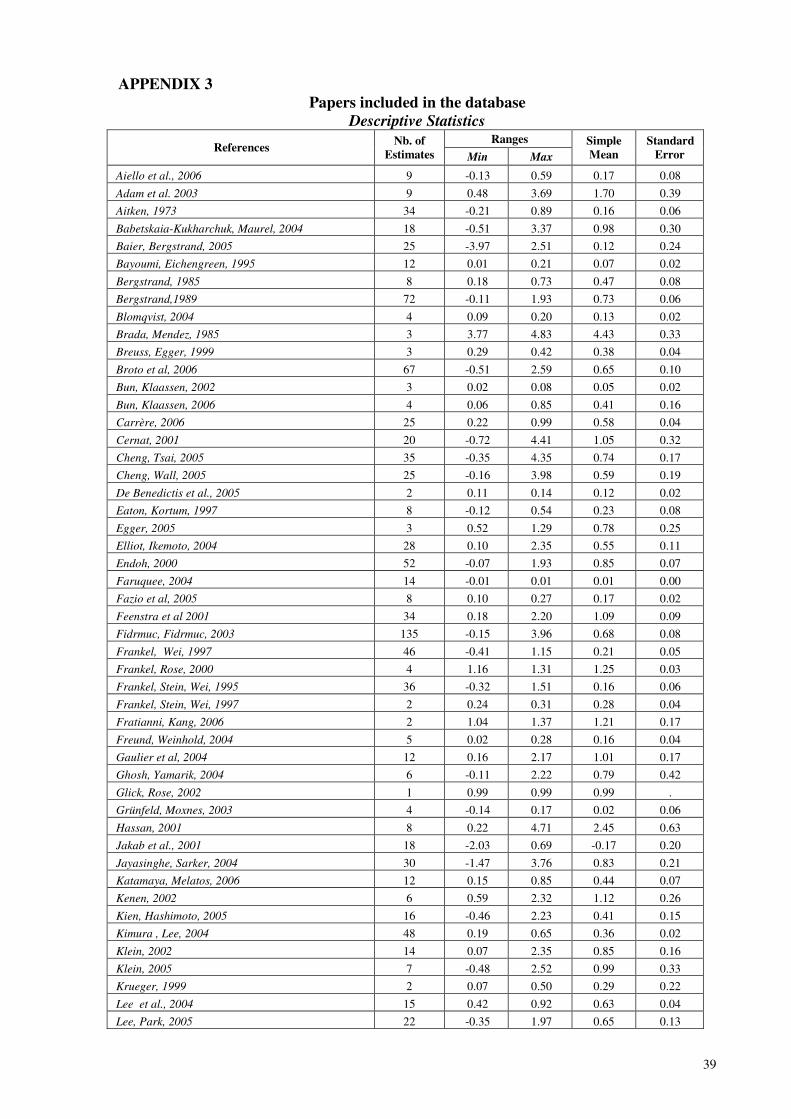
39

APPENDIX 3

Papers included in the database

Descriptive Statistics Ranges

References Nb. of

Estimates Min Max

Simple

Mean

Standard

Error

Aiello et al., 2006 9 -0.13 0.59 0.17 0.08

Adam et al. 2003 9 0.48 3.69 1.70 0.39

Aitken, 1973 34 -0.21 0.89 0.16 0.06

Babetskaia-Kukharchuk, Maurel, 2004 18 -0.51 3.37 0.98 0.30

Baier, Bergstrand, 2005 25 -3.97 2.51 0.12 0.24

Bayoumi, Eichengreen, 1995 12 0.01 0.21 0.07 0.02

Bergstrand, 1985 8 0.18 0.73 0.47 0.08

Bergstrand,1989 72 -0.11 1.93 0.73 0.06

Blomqvist, 2004 4 0.09 0.20 0.13 0.02

Brada, Mendez, 1985 3 3.77 4.83 4.43 0.33

Breuss, Egger, 1999 3 0.29 0.42 0.38 0.04

Broto et al, 2006 67 -0.51 2.59 0.65 0.10

Bun, Klaassen, 2002 3 0.02 0.08 0.05 0.02

Bun, Klaassen, 2006 4 0.06 0.85 0.41 0.16

Carrère, 2006 25 0.22 0.99 0.58 0.04

Cernat, 2001 20 -0.72 4.41 1.05 0.32

Cheng, Tsai, 2005 35 -0.35 4.35 0.74 0.17

Cheng, Wall, 2005 25 -0.16 3.98 0.59 0.19

De Benedictis et al., 2005 2 0.11 0.14 0.12 0.02

Eaton, Kortum, 1997 8 -0.12 0.54 0.23 0.08

Egger, 2005 3 0.52 1.29 0.78 0.25

Elliot, Ikemoto, 2004 28 0.10 2.35 0.55 0.11

Endoh, 2000 52 -0.07 1.93 0.85 0.07

Faruquee, 2004 14 -0.01 0.01 0.01 0.00

Fazio et al, 2005 8 0.10 0.27 0.17 0.02

Feenstra et al 2001 34 0.18 2.20 1.09 0.09

Fidrmuc, Fidrmuc, 2003 135 -0.15 3.96 0.68 0.08

Frankel, Wei, 1997 46 -0.41 1.15 0.21 0.05

Frankel, Rose, 2000 4 1.16 1.31 1.25 0.03

Frankel, Stein, Wei, 1995 36 -0.32 1.51 0.16 0.06

Frankel, Stein, Wei, 1997 2 0.24 0.31 0.28 0.04

Fratianni, Kang, 2006 2 1.04 1.37 1.21 0.17

Freund, Weinhold, 2004 5 0.02 0.28 0.16 0.04

Gaulier et al, 2004 12 0.16 2.17 1.01 0.17

Ghosh, Yamarik, 2004 6 -0.11 2.22 0.79 0.42

Glick, Rose, 2002 1 0.99 0.99 0.99 .

Grünfeld, Moxnes, 2003 4 -0.14 0.17 0.02 0.06

Hassan, 2001 8 0.22 4.71 2.45 0.63

Jakab et al., 2001 18 -2.03 0.69 -0.17 0.20

Jayasinghe, Sarker, 2004 30 -1.47 3.76 0.83 0.21

Katamaya, Melatos, 2006 12 0.15 0.85 0.44 0.07

Kenen, 2002 6 0.59 2.32 1.12 0.26

Kien, Hashimoto, 2005 16 -0.46 2.23 0.41 0.15

Kimura , Lee, 2004 48 0.19 0.65 0.36 0.02

Klein, 2002 14 0.07 2.35 0.85 0.16

Klein, 2005 7 -0.48 2.52 0.99 0.33

Krueger, 1999 2 0.07 0.50 0.29 0.22

Lee et al., 2004 15 0.42 0.92 0.63 0.04

Lee, Park, 2005 22 -0.35 1.97 0.65 0.13

40

Lennon, 2006 16 -0.20 0.41 0.07 0.03

Màrquez-Ramos et al., 2006 40 -0.21 5.23 2.03 0.26

Martìnez-Galàn et al, 2005 4 -0.06 0.00 -0.02 0.01

Martìnez-Zarzoso, Horsewood, 2005 48 0.01 2.63 0.77 0.11

Martìnez-Zarzoso, Nowak-Lehmann, 2003 28 0.04 0.65 0.24 0.03

Mayer, Zignago, 2005 12 0.72 2.30 1.78 0.16

Meliz, 2001 4 1.03 1.24 1.16 0.05

Meliz, 2002 3 1.00 1.02 1.01 0.01

Micco et at, 2003 43 -0.30 0.18 0.01 0.01

Nitsch, 2002 15 0.68 1.28 1.07 0.05

Paiva, 2005 5 1.01 1.15 1.10 0.02

Pakko, Wall, 2001 6 0.05 0.91 0.43 0.17

Papazoglou et al., 2006 2 0.29 0.33 0.31 0.02

Rauch, 1996 72 -1.18 1.11 0.03 0.06

Rauch, Trindade, 1999 48 -0.64 0.46 0.07 0.04

Rose, 2000 53 -0.97 1.54 0.79 0.06

Rose, 2004 6 0.94 1.50 1.19 0.07

Rose, 2005a 17 0.07 0.75 0.53 0.05

Rose, 2005b 4 -0.07 -0.02 -0.05 0.01

Rose, Engel, 2002 4 0.75 0.95 0.88 0.04

Rose, van Wincoop, 2001 2 0.46 1.09 0.78 0.32

Saiki, 2005 4 0.73 1.66 1.24 0.22

Sanso et al., 1993 28 -0.05 1.32 0.34 0.07

Sapir, 2001 33 -0.54 0.34 0.01 0.05

Siliverstovs and Schumacher, 2006 174 -1.89 1.77 0.08 0.04

Silva, Tenreyro, 2003 6 0.26 0.79 0.44 0.11

Silva, Tenreyro, 2005 12 0.14 1.29 0.48 0.10

Sissoko, 2004 27 0.21 2.64 1.57 0.15

Subramanian, Wei 2003 30 0.18 1.99 0.89 0.08

Subramanian, Wei 2005 30 -0.13 1.99 0.92 0.09

Tang, 2005 10 0.26 1.83 0.80 0.19

Tenreyro, 2001 4 0.29 0.70 0.53 0.09

Thom, Walsh, 2002 20 -0.10 0.74 0.11 0.06

Verdeja, 2005 15 -1.38 1.90 0.39 0.23

Walsh, 2006 16 -9.01 15.41 4.35 1.69

Yeyati, 2003 10 0.47 1.00 0.58 0.05

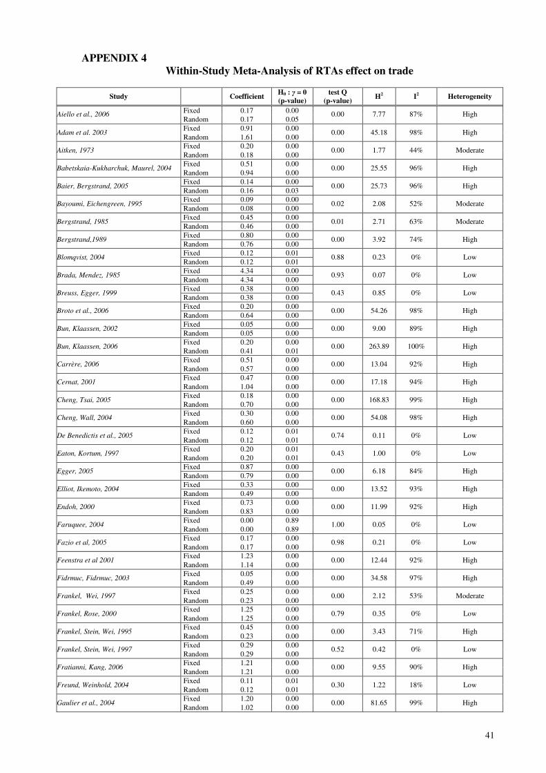
41

APPENDIX 4

Within-Study Meta-Analysis of RTAs effect on trade

Study Coefficient H0 : γ = 0

(p-value) test Q

(p-value) H2 I2 Heterogeneity

Fixed 0.17 0.00 Aiello et al., 2006

Random 0.17 0.05 0.00 7.77 87% High

Fixed 0.91 0.00 Adam et al. 2003

Random 1.61 0.00 0.00 45.18 98% High

Fixed 0.20 0.00 Aitken, 1973

Random 0.18 0.00 0.00 1.77 44% Moderate

Fixed 0.51 0.00 Babetskaia-Kukharchuk, Maurel, 2004

Random 0.94 0.00 0.00 25.55 96% High

Fixed 0.14 0.00 Baier, Bergstrand, 2005

Random 0.16 0.03 0.00 25.73 96% High

Fixed 0.09 0.00 Bayoumi, Eichengreen, 1995

Random 0.08 0.00 0.02 2.08 52% Moderate

Fixed 0.45 0.00 Bergstrand, 1985

Random 0.46 0.00 0.01 2.71 63% Moderate

Fixed 0.80 0.00 Bergstrand,1989

Random 0.76 0.00 0.00 3.92 74% High

Fixed 0.12 0.01 Blomqvist, 2004

Random 0.12 0.01 0.88 0.23 0% Low

Fixed 4.34 0.00 Brada, Mendez, 1985

Random 4.34 0.00 0.93 0.07 0% Low

Fixed 0.38 0.00 Breuss, Egger, 1999

Random 0.38 0.00 0.43 0.85 0% Low

Fixed 0.20 0.00 Broto et al., 2006

Random 0.64 0.00 0.00 54.26 98% High

Fixed 0.05 0.00 Bun, Klaassen, 2002

Random 0.05 0.00 0.00 9.00 89% High

Fixed 0.20 0.00 Bun, Klaassen, 2006

Random 0.41 0.01 0.00 263.89 100% High

Fixed 0.51 0.00 Carrère, 2006

Random 0.57 0.00 0.00 13.04 92% High

Fixed 0.47 0.00 Cernat, 2001

Random 1.04 0.00 0.00 17.18 94% High

Fixed 0.18 0.00 Cheng, Tsai, 2005

Random 0.70 0.00 0.00 168.83 99% High

Fixed 0.30 0.00 Cheng, Wall, 2004

Random 0.60 0.00 0.00 54.08 98% High

Fixed 0.12 0.01 De Benedictis et al., 2005

Random 0.12 0.01 0.74 0.11 0% Low

Fixed 0.20 0.01 Eaton, Kortum, 1997

Random 0.20 0.01 0.43 1.00 0% Low

Fixed 0.87 0.00 Egger, 2005

Random 0.79 0.00 0.00 6.18 84% High

Fixed 0.33 0.00 Elliot, Ikemoto, 2004

Random 0.49 0.00 0.00 13.52 93% High

Fixed 0.73 0.00 Endoh, 2000

Random 0.83 0.00 0.00 11.99 92% High

Fixed 0.00 0.89 Faruquee, 2004

Random 0.00 0.89 1.00 0.05 0% Low

Fixed 0.17 0.00 Fazio et al, 2005

Random 0.17 0.00 0.98 0.21 0% Low

Fixed 1.23 0.00 Feenstra et al 2001

Random 1.14 0.00 0.00 12.44 92% High

Fixed 0.05 0.00 Fidrmuc, Fidrmuc, 2003

Random 0.49 0.00 0.00 34.58 97% High

Fixed 0.25 0.00 Frankel, Wei, 1997

Random 0.23 0.00 0.00 2.12 53% Moderate

Fixed 1.25 0.00 Frankel, Rose, 2000

Random 1.25 0.00 0.79 0.35 0% Low

Fixed 0.45 0.00 Frankel, Stein, Wei, 1995

Random 0.23 0.00 0.00 3.43 71% High

Fixed 0.29 0.00 Frankel, Stein, Wei, 1997

Random 0.29 0.00 0.52 0.42 0% Low

Fixed 1.21 0.00 Fratianni, Kang, 2006

Random 1.21 0.00 0.00 9.55 90% High

Fixed 0.11 0.01 Freund, Weinhold, 2004

Random 0.12 0.01 0.30 1.22 18% Low

Fixed 1.20 0.00 Gaulier et al., 2004

Random 1.02 0.00 0.00 81.65 99% High

42

Fixed 0.38 0.00 Ghosh, Yamarik, 2004

Random 0.74 0.03 0.00 47.34 98% High

Fixed 0.99 0.00 Glick, Rose, 2002

Random 0.99 0.00 -

-

-

-

Fixed 0.03 0.70 Grünfeld, Moxnes, 2003

Random 0.03 0.70 0.56 0.70 0% Low

Fixed 2.61 0.00 Hassan, 2001

Random 2.61 0.00 0.44 0.99 0% Low

Fixed -0.44 0.00 Jakab et al., 2001

Random -0.18 0.15 0.00 484.32 100% High

Fixed 0.69 0.00 Jayasinghe, Sarker, 2004

Random 0.81 0.00 0.00 4.71 79% High

Fixed 0.54 0.00 Katamaya, Melatos, 2006

Random 0.45 0.00 0.00 16.15 94% High

Fixed 0.76 0.00 Kenen, 2002

Random 0.86 0.00 0.07 2.05 51% Moderate

Fixed 0.19 0.00 Kien, Hashimoto, 2005

Random 0.41 0.01 0.00 92.81 99% High

Fixed 0.37 0.00 Kimura , Lee, 2004

Random 0.37 0.00 0.44 1.02 2% Low

Fixed 0.87 0.00 Klein, 2002

Random 0.87 0.00 0.01 2.15 54% Moderate

Fixed 1.06 0.00 Klein, 2005

Random 1.04 0.00 0.00 6.12 84% High

Fixed 0.10 0.13 Krueger, 1999

Random 0.21 0.29 0.10 2.65 62% Moderate

Fixed 0.56 0.00 Lee et al., 2004

Random 0.62 0.00 0.00 14.64 93% High

Fixed 0.51 0.00 Lee, Park, 2005

Random 0.62 0.00 0.00 20.63 95% High

Fixed 0.09 0.00 Lennon. 2006

Random 0.08 0.01 0.00 6.16 84% High

Fixed 0.89 0.00 Màrquez-Ramos et al., 2006

Random 1.82 0.00 0.00 29.99 97% High

Fixed -0.02 0.81 Martìnez-Galàn et al, 2005

Random -0.02 0.81 1.00 0.02 0% Low

Fixed 0.16 0.00 Martìnez-Zarzoso, Horsewood, 2005

Random 0.61 0.00 0.00 26.42 96% High

Fixed 0.06 0.00 Martìnez-Zarzoso, Nowak-Lehmann,

2003 Random 0.18 0.00 0.00 22.63 96% High

Fixed 1.60 0.00 Mayer, Zignago, 2005

Random 1.76 0.00 0.00 35.81 97% High

Fixed 1.16 0.00 Meliz, 2001

Random 1.16 0.00 0.45 0.88 0% Low

Fixed 1.01 0.00 Meliz, 2002

Random 1.01 0.00 0.99 0.01 0% Low

Fixed 0.02 0.00 Micco et at, 2003

Random 0.02 0.04 0.00 2.57 61% Moderate

Fixed 1.06 0.00 Nitsch, 2002

Random 1.07 0.00 0.08 1.56 36% Low

Fixed 1.10 0.00 Paiva, 2005

Random 1.10 0.00 0.85 0.34 0% Low

Fixed 0.53 0.00 Pakko, Wall, 2001

Random 0.43 0.01 0.00 17.29 94% High

Fixed 0.30 0.00 Papazoglou et al., 2006

Random 0.30 0.00 0.84 0.04 0% Low

Fixed 0.03 0.35 Rauch, 1996

Random 0.04 0.47 0.00 3.15 68% Moderate

Fixed 0.10 0.00 Rauch, Trindade, 1999

Random 0.10 0.01 0.01 1.54 35% Low

Fixed 0.10 0.00 Rose, 2000

Random 0.83 0.00 0.00 85.65 99% High

Fixed 1.18 0.00 Rose, 2004

Random 1.18 0.00 0.13 1.69 41% Moderate

Fixed 0.60 0.00 Rose, 2005a

Random 0.54 0.00 0.00 9.53 90% High

Fixed -0.04 0.00 Rose, 2005b

Random -0.04 0.00 0.47 0.85 0% Low

Fixed 0.88 0.00 Rose, Engel, 2002

Random 0.88 0.00 0.79 0.35 0% Low

Fixed 0.83 0.00 Rose, van Wincoop, 2001

Random 0.78 0.01 0.00 16.27 94% High

Fixed 0.97 0.00 Saiki, 2005

Random 1.15 0.00 0.01 4.23 76% High

Sanso et al., 1993 Fixed 0.32 0.00 0.00 7.17 86% High

43

Random 0.35 0.00 Fixed -0.02 0.68

Sapir, 2001 Random -0.01 0.90

0.02 1.55 36% Low

Fixed 0.25 0.00 Siliverstovs, Schumacher, 2006

Random 0.13 0.00 0.00 5.35 81% High

Fixed 0.35 0.00 Silva, Tenreyro, 2003

Random 0.42 0.00 0.00 5.34 81% High

Fixed 0.41 0.00 Silva, Tenreyro, 2005

Random 0.46 0.00 0.00 8.99 89% High

Fixed 1.48 0.00 Sissoko, 2004

Random 1.46 0.00 0.00 1.99 50% Moderate

Fixed 0.86 0.00 Subramanian, Wei 2003

Random 0.88 0.00 0.00 7.42 87% High

Fixed 0.89 0.00 Subramanian, Wei 2005

Random 0.92 0.00 0.00 9.83 90% High

Fixed 0.75 0.00 Tang, 2005

Random 0.80 0.00 0.00 17.95 94% High

Fixed 0.53 0.00 Tenreyro, 2001

Random 0.53 0.00 0.00 5.24 81% High

Fixed 0.04 0.00 Thom, Walsh, 2002

Random 0.10 0.00 0.00 18.40 95% High

Fixed 0.37 0.00 Verdeja, 2005

Random 0.45 0.02 0.00 5.72 83% High

Fixed 0.31 0.00 Walsh, 2006

Random 0.47 0.01 0.01 2.16 54% Moderate

Fixed 0.58 0.00 Yeyati, 2003

Random 0.58 0.00 0.05 1.91 48% Moderate