recognizing semantics in human actions with object detectionann/exjobb/oscar_friberg.pdf ·...
TRANSCRIPT

Recognizing Semantics inHuman Actions with ObjectDetection
OSCAR FRIBERG
Master in Computer ScienceDate: June 9, 2017Supervisor: Atsuto MakiExaminer: Hedvig KjellströmSwedish title: Igenkänning av Semantik i Mänsklig Handling medObjektdetektionSchool of Computer Science and Communication


iii
Abstract
Recent work in human action recognition in videos seeks to further ex-tend a two-stream convolutional network framework. The two-streamconvolutional networks separates spatial and temporal informationinto two separate networks. There has been some attempts to com-plement the two networks with a third network with auxiliary infor-mation.
We make two contributions in this thesis. First we show that se-mantics using objects detections as a third network with the two-streamconvolutional networks can provide slight improvements for humanaction recognition on standard benchmarks.
Secondly, we attempt to seek a few ways to force our new seman-tic network to diverge from the other two streams with a few diver-gence terms. Slight gains are seen using these divergence boostingtechniques.

iv
Sammanfattning
Senaste arbete inom mänsklig handlingsigenkänning i film har söktolika tillvägagångssätt att utöka ett ramverk för faltningsnätverk i tvåströmmar. De två strömmarna separerar rumslig och timlig informa-tion i två separata nätverk. Det har varit några försök att komplemen-tera dessa två nätverk med ett tredje nätverk med extra information.
Vi gör två bidrag i detta examensarbete. Först vi visar att seman-tik med objektdetektion som ett tredje nätverk tillsammans med falt-ningsnätverk i två strömmar kan bidra till små förbättringar till mänsk-lig handlingsigenkänning i videos på riktmärkesstandarder.
För det andra söker vi efter olika sätt att tvinga vår nya semantiskanätverk att divergera från the andra två strömmarna genom att läggatill divergenstermer. Vi ser små förbättringar med att använda dessatekniker för att öka divergens.

Contents
1 Introduction 11.1 Problem Statement . . . . . . . . . . . . . . . . . . . . . . 2
2 Background 32.1 Rise of Convolutional Neural Networks . . . . . . . . . . 32.2 Image Recognition . . . . . . . . . . . . . . . . . . . . . . 42.3 Human Action Recognition in Videos . . . . . . . . . . . 5
2.3.1 Datasets for Human Action Recognition . . . . . . 62.4 Object Detection Systems . . . . . . . . . . . . . . . . . . . 72.5 Related Work . . . . . . . . . . . . . . . . . . . . . . . . . 8
3 Deep Learning Introduction 103.1 Machine Learning . . . . . . . . . . . . . . . . . . . . . . . 10
3.1.1 Supervised Learning . . . . . . . . . . . . . . . . . 113.1.2 Unsupervised Learning . . . . . . . . . . . . . . . 113.1.3 Regression . . . . . . . . . . . . . . . . . . . . . . . 113.1.4 Classification . . . . . . . . . . . . . . . . . . . . . 13
3.2 Deep Convolutional Networks . . . . . . . . . . . . . . . 153.2.1 Fully Connected Layers . . . . . . . . . . . . . . . 163.2.2 Convolutional Layers . . . . . . . . . . . . . . . . 173.2.3 Batch Normalization . . . . . . . . . . . . . . . . . 203.2.4 Dropout . . . . . . . . . . . . . . . . . . . . . . . . 20
3.3 Parameter Optimization . . . . . . . . . . . . . . . . . . . 213.3.1 Categorical Crossentropy . . . . . . . . . . . . . . 213.3.2 Gradient Descent . . . . . . . . . . . . . . . . . . . 213.3.3 Stochastic Gradient Descent . . . . . . . . . . . . . 223.3.4 Weight Decay . . . . . . . . . . . . . . . . . . . . . 233.3.5 Transfer Learning . . . . . . . . . . . . . . . . . . . 23
v

vi CONTENTS
4 Human Action Recognition 254.1 Two-Stream Convolutional Networks . . . . . . . . . . . 25
4.1.1 VGG16 - A Very Deep Convolutional Network . . 274.1.2 Optical Flow . . . . . . . . . . . . . . . . . . . . . . 274.1.3 Spatial Stream . . . . . . . . . . . . . . . . . . . . . 274.1.4 Temporal Stream . . . . . . . . . . . . . . . . . . . 28
4.2 Object Detection . . . . . . . . . . . . . . . . . . . . . . . . 284.2.1 YOLO — You Only Look Once . . . . . . . . . . . 284.2.2 SSD — Single Shot MultiBox Detector . . . . . . . 33
4.3 Semantic Stream . . . . . . . . . . . . . . . . . . . . . . . . 334.3.1 Where to connect YOLO . . . . . . . . . . . . . . . 354.3.2 Where to connect SSD . . . . . . . . . . . . . . . . 364.3.3 Architecture of Semantic Stream . . . . . . . . . . 364.3.4 Fusion of Streams . . . . . . . . . . . . . . . . . . . 37
4.4 Boosting Divergence . . . . . . . . . . . . . . . . . . . . . 374.4.1 Average Layer . . . . . . . . . . . . . . . . . . . . . 374.4.2 Kullback-Leibler Divergence . . . . . . . . . . . . 384.4.3 Dot Product Divergence . . . . . . . . . . . . . . . 384.4.4 Combining Average with Divergence . . . . . . . 39
4.5 Implementation Details . . . . . . . . . . . . . . . . . . . . 394.5.1 Training . . . . . . . . . . . . . . . . . . . . . . . . 394.5.2 Datasets . . . . . . . . . . . . . . . . . . . . . . . . 404.5.3 Evaluation . . . . . . . . . . . . . . . . . . . . . . . 414.5.4 Equipment . . . . . . . . . . . . . . . . . . . . . . . 41
5 Results 425.1 Setting up the Spatial and the Temporal Streams . . . . . 425.2 Objects Detected in Clips . . . . . . . . . . . . . . . . . . . 435.3 Experiments . . . . . . . . . . . . . . . . . . . . . . . . . . 44
5.3.1 Where to Connect the Semantic Stream . . . . . . 445.3.2 Dropout Rates . . . . . . . . . . . . . . . . . . . . . 445.3.3 Adding Additional Hidden Layers . . . . . . . . . 475.3.4 Divergence Boosting . . . . . . . . . . . . . . . . . 485.3.5 Experiments on HMDB-51 . . . . . . . . . . . . . . 495.3.6 Mean Accuracy over all Three Splits . . . . . . . . 505.3.7 Per Class Accuracy . . . . . . . . . . . . . . . . . . 50

CONTENTS vii
6 Discussion 566.1 Comparison of Object Detection Systems . . . . . . . . . 566.2 Comparison with State-of-the-Art . . . . . . . . . . . . . . 566.3 Directions of Improvement . . . . . . . . . . . . . . . . . 57
6.3.1 Temporal Setting . . . . . . . . . . . . . . . . . . . 576.3.2 Very Deep Semantic Streams . . . . . . . . . . . . 586.3.3 Further Investigations on Divergence Boosting . . 586.3.4 More Object Categories . . . . . . . . . . . . . . . 59
7 Conclusion 60
Bibliography 61
A Dataset Classes 68A.1 HMDB-51 . . . . . . . . . . . . . . . . . . . . . . . . . . . 68A.2 UCF-101 . . . . . . . . . . . . . . . . . . . . . . . . . . . . 69A.3 COCO . . . . . . . . . . . . . . . . . . . . . . . . . . . . . 70


Chapter 1
Introduction
What kind of features are essential for recognizing different humanactions? This is a natural question to ask when designing human ac-tion recognition systems. Human action recognition is the problem ofrecognizing what kind of human action is represented in a video clip.One can see this as an extension of image recognition, which concernsabout what kind of object is represented in an image.
One could argue that a temporal awareness is essential for humanaction recognition. For example, a still image of a person about tosit down might look indistinguishable from a still image of a personstanding up from a sitting position. But if we are able to see the motionof the person in multiple consecutive frames, we will probably be ableto deduce if the person in sitting down or standing up.
Of course, while temporal awareness is important for action recog-nition, a spatial awareness can be important too. Some actions are of-ten made in a certain environment. For example, an action is probablyrelated to cooking or eating if we know the action is made in a kitchen.
The current state-of-the-art for human action recognition combinesthe spatial information with the temporal information of the video[14]. These models consists of one stream for spatial information andone stream for temporal information, and are therefore called a two-stream model.
It is natural to ask if there are any other information that can helpto understand human action recognition. One example that has beeninvestigated recently with some success is pose information [63].
In this thesis we investigate if the awareness of the location of dif-ferent objects are important for human action recognition.
1

2 CHAPTER 1. INTRODUCTION
For example, if a hammer is detected close to a person, the actionis probably hammering. Another example is an action is likely to berelated to riding a horse if a person is detected above a horse.
Object detection systems are nowadays very efficient. Some of thefastest systems are not much slower than image recognition. This al-lows us to use object detection systems.
1.1 Problem Statement
The question this thesis investigates is if object detection systems cancomplement the two-stream model for human action recognition invideos? We seek to answer this question by implementing a semanticstream which maps object detection features to human action recogni-tion classes.

Chapter 2
Background
2.1 Rise of Convolutional Neural Networks
Computer vision has changed in a rapid pace the past few years withthe rise of convolutional neural networks. The popularity of convolu-tional neural networks started when it was proven to be effective onlarge image recognition benchmarks such as ImageNet [25]. Ever sincethen, convolutional neural networks have been used to win multiplecompetitions [19].
Even if convolutional neural networks made its breakthrough withimage recognition, researchers have found it to be useful for othercomputer vision applications as well. For example, convolutional neu-ral networks have been used to generate captions to images and videos[56] [13] [23], generate sound for silent videos [38] and even generatecolorized images from grayscale images [6]. Convolutional neural net-works have even found use in applications beyond computer vision,such as evaluating board positions and moves for a champion level GoAI [49]. The possibilities are seemingly endless.
Convolutional neural networks are not a new invention. It has beenused even early as the 1990s for image recognition problems [33]. Thereason why convolutional neural networks became popular just thisdecade is due to the introduction of large-scale public repositories suchas ImageNet, which made it possible to train deep convolutional neu-ral networks [10].
Also, another part of the increased popularity is the increased com-puting power capacity and accessibility to advanced computing equip-ment such as GPUs. Training convolutional neural networks on GPUs
3

4 CHAPTER 2. BACKGROUND
can be faster than CPU training by a factor 10 [48]. The advancementof computing equipment has allowed to stack multiple convolutionallayers in a deep network.
2.2 Image Recognition
Image recognition, or image classification, is the problem to label animage by its contents. A typical example of a simple image recogni-tion problem is digit recognition in the MNIST database of handwrit-ten digits [32]; decide which digit is represented in an image. Morecomplex image recognition problems, such as ImageNet ILSVRC-2012classification task, an image recognition system has to correctly label50,000 images into 1,000 categories [46].
The raw pixel values of images are often very high dimensional.For example, the image space of a square RGB image with size 256 has256 × 256 × 3 = 196, 608 dimensions. However, this many degrees offreedom for the image features is probably unnecessary for an imagerecognition problem. A random sample of a image space is likely justrandom noise with no valuable information.
It is therefore a common practice to project the features of the im-ages to a lower dimensional space to make image recognition moreviable. This lower dimensional space should ideally a good repre-sentation of the image features and contain as much valuable infor-mation as possible. Traditional face recognition methods like Eigen-faces projects the input to a linear subspace with Principal ComponentAnalysis (PCA) [2].
Another practice to make classification more viable is to change thedescriptor of the image. The typical RGB descriptor is good for repre-senting the colors of the image, but does not necessarily represent theshapes or the structure of the image. Histogram of Oriented Gradients(HOG) is a hand-crafted descriptor which is better at representing thestructural properties of an image. HOG has been used for traditionalimage recognition tasks [12]. The HOG-descriptor maps the imageinto a HOG-space where local gradients of the image is represented.
But convolutional neural networks have made both handcraftedrepresentations and descriptors such as HOG obsolete for image recog-nition. Instead of using hand-crafted representations, convolutionalneural networks are used to learns the representation directly from the

CHAPTER 2. BACKGROUND 5
RGB features of the image. Seemingly convolutional neural networksare flexible enough to learn representations by itself. It has even beenshown that handcrafted features such as HOG can be interpreted ascorresponding to a part of convolutional neural networks [29].
2.3 Human Action Recognition in Videos
Human action recognition in videos is the problem to recognize whatkind of human action is played in a video. Examples of human actionsto recognize can be simple actions such as handwaving, walking orjumping, or more advanced actions such as playing basketball, salsadancing or tai chi.
Even if human action recognition is seemingly similar to imagerecognition, convolutional neural networks have not so far benefitedhuman action recognition over hand-crafted video representation sub-stantially.
Dense trajectories is a hand-crafted video representation which hasbeen proven successful for action recognition [58]. Dense trajectorieswas introduced for instance in [57], and uses optical flow fields to trackdensely sampled points. Another hand-crafted approach uses densetrajectories together with bag of visual words with great success [40].
3D convolutional neural networks have been used to combine thespatial and the temporal features of the input in the same model forhuman action recognition. However, 3D convolutional neural net-works have only led to a very small success [22]. A possible reasonfor the small success is that the available datasets for human actionrecognition are currently too small to properly learn the 3D convolu-tional neural networks.
Combining the predictions of 2D convolutional neural networksfrom a sequence of frames has also been tried. [24] proposes differentstrategies to combine the predictions of convolutional neural networksfrom multiple frames, and concluded a slow-fusion approach is themost effective.
One of the most successful approaches of using convolutional neu-ral networks for human action recognition divides the spatial and thetemporal features into two separate networks, commonly known astwo-stream networks [50]. Two-stream networks separately learns thefeatures of the RGB frames and the optical flow of the videos. This

6 CHAPTER 2. BACKGROUND
is inspired by observations in how the brain recognizes actions. Evi-dently, the RGB frames and the optical flow of a video provides com-plementary predictions for human action recognition.
Recurrent neural networks, commonly used for sequential data,have also been considered for action recognition. Long short-termmemory (LSTM) is a specific type of recurrent neural network provento be capable of large-scale learning of speech recognition and othernatural language processing problems [20] [55].
The original two-stream approach predicts on a single-frame basis.In its standard form it is unable to model temporal structures, andthere are some attempts to cope with this issue. LSTM has been usedto extend the two-stream approach to accept sequential data, with anobserved improvement over the single-frame baseline [13].
Another way to cope with modeling temporal structures with two-stream networks by deriving the consensus between sampled snippetsof the clip [59]. For each of the snippets an action is predicted usingthe two streams. The predictions are then combined by deriving theconsensus among the prediction. This is to our knowledge the bestapproach achieved on UCF-101 with 94.2%.
2.3.1 Datasets for Human Action Recognition
As human action recognition in videos has progressed, the demandfor more complex datasets has increased. Early datasets, like the KTH[30] and the Weizmann dataset[3], were small and in very constrainedenvironment. The KTH dataset contains six different types of actionsperformed by 25 subjects in four different environments. The camerais static and filmed so the full body of the subjects are visible. Thebackground of the videos are also free from any kind of eventual dis-tractions.
The Weizmann dataset is very similar to the KTH dataset, but isless constrained by letting the subjects to be in more complex environ-ments. However, the actions are still very simple and constrained.
UCF-Sports is a dataset with sport actions collected from variousTV broadcasts [45]. This dataset is more challenging than the previ-ous datasets due to be in a much less constrained setting with vari-ous camera angles, lighting, backgrounds. Similarly, the Hollywooddataset collects different human actions from Hollywood movies [31].This dataset also includes shots within clips.

CHAPTER 2. BACKGROUND 7
Figure 2.4.1: Example of a traditional sliding windows approach forobject detection. First a classifier is used on windows of different sizesat different locations of the image. Regions yielding probable detec-tions are proposed. Possible duplicates are ruled out so only the bestdetection is used. Nowadays a single convolutional network can beused to get the detections directly.
The two most common datasets for human action recognition asof today are UCF-101 [52] and HMDB-51 [27]. Both datasets are col-lections of human actions from many different kinds of sources, liketelevision programs, internet videos and feature films.
2.4 Object Detection Systems
While human action recognition has not enjoyed the same leap in progressas image recognition, object detection systems have surprisingly ben-efited very well by convolutional neural networks.
Traditional object detection systems, like ensemble of exemplar-svms or deformable parts models (DPM), used a sliding window ap-proach for object detection [36] [15]. These approaches finds the ob-jects in a image by running a classifier at evenly spaced locations overthe entire image. Only one classifier needs to be learned for the slid-ing window approach. However, using sliding windows is very costlysince a classifier has to be used many times for each image, whichmakes real-time detections very difficult with this approach.
More recent approaches, like Faster R-CNN, avoids the sliding win-dow approach by using a convolutional neural network for proposingthe regions of the objects [44]. After proposing the regions and rulingout possible duplicates, a classifier is run over each region proposal toget the class scores. The downside of approaches like Faster R-CNNis that two networks needs to learned. One network for proposing re-gions and another for classifying the proposed regions. Faster R-CNN
8 CHAPTER 2. BACKGROUND
is also slower than real-time even on powerful GPUs like Geforce GTXTitan X [43].
The object dection system You Only Look Once (YOLO) on theother hand, proved it is possible to unify the region proposal and classscore prediction in one single convolutional neural network. This uni-fied network is much simpler to optimize than Faster R-CNN since theobject detection can be framed as a regression problem. Faster R-CNNrequires that multiple components in a complex pipeline are trainedseparately [42]. The single convolutional neural network architecturealso allows YOLO to achieve a real-time performance.
YOLO has been improved upon it first original introduction in asecond version, YOLOv2 [43]. YOLOv2 is similar to the original ver-sion, but some adjustments in the model makes it both more accurateand faster. Single Shot Multibox Detector (SSD) is another networkwhich follows the success of YOLO by performing object detections inone single convolutional neural network [35].
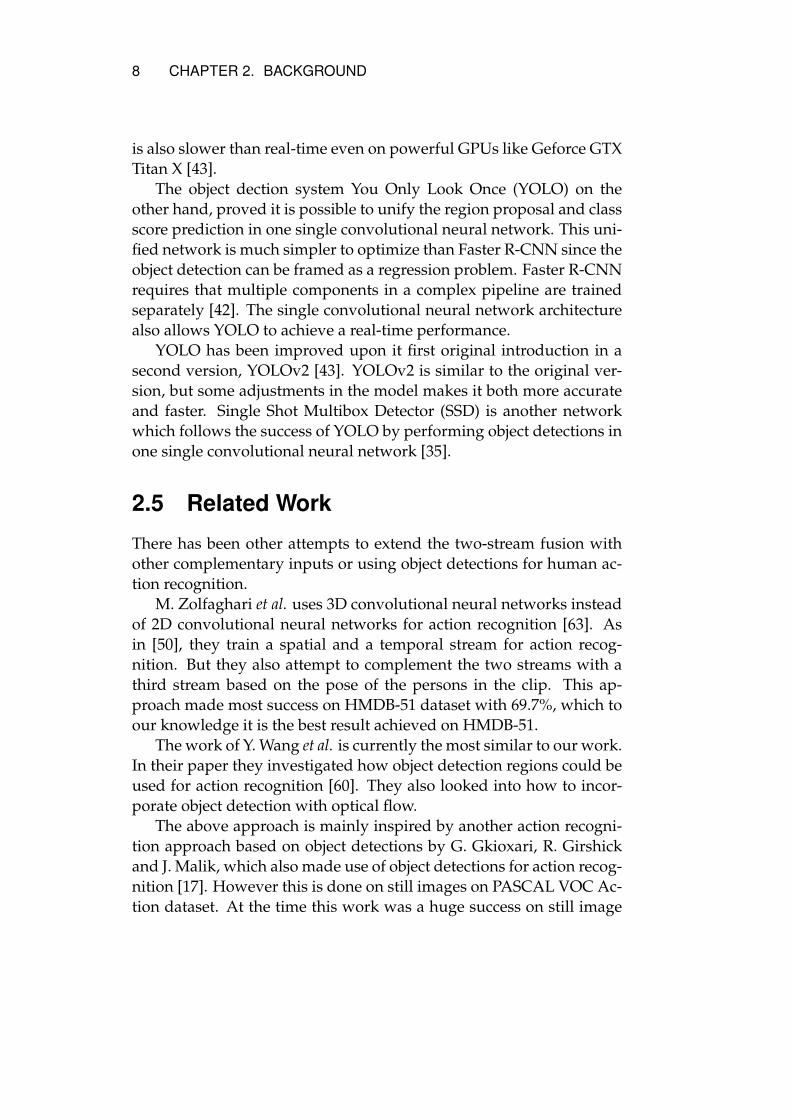
2.5 Related Work
There has been other attempts to extend the two-stream fusion withother complementary inputs or using object detections for human ac-tion recognition.
M. Zolfaghari et al. uses 3D convolutional neural networks insteadof 2D convolutional neural networks for action recognition [63]. Asin [50], they train a spatial and a temporal stream for action recog-nition. But they also attempt to complement the two streams with athird stream based on the pose of the persons in the clip. This ap-proach made most success on HMDB-51 dataset with 69.7%, which toour knowledge it is the best result achieved on HMDB-51.
The work of Y. Wang et al. is currently the most similar to our work.In their paper they investigated how object detection regions could beused for action recognition [60]. They also looked into how to incor-porate object detection with optical flow.
The above approach is mainly inspired by another action recogni-tion approach based on object detections by G. Gkioxari, R. Girshickand J. Malik, which also made use of object detections for action recog-nition [17]. However this is done on still images on PASCAL VOC Ac-tion dataset. At the time this work was a huge success on still image

CHAPTER 2. BACKGROUND 9
action recognition.Our contribution differentiates from the above approaches by only
looking at the location and the target class of the bounding boxes. Wedo not make a decision based on the contents of the regions.

Chapter 3
Deep Learning Introduction
This chapter serves as a quick introduction to the deep learning tech-niques used in this paper. No prior knowledge of machine learningtechniques is required for reading this chapter.
Section 3.1 discusses the machine learning techniques which areimportant for this paper. For human action recognition we want theprogram to understand how to distinguish different actions in videos,which is normally done with machine learning. Section 3.2 continuesby describing common layers used for deep convolutional networks.Finally section 3.3 discusses how the parameters of the deep convolu-tional network can be optimized in a classification setting.
3.1 Machine Learning
Machine learning is a common name of techniques that learn fromdata. Many problems are difficult to solve directly programmaticallyby hand. For example, imagine to program by hand a system that rec-ognizes a cat in an image. A cat can look in many different ways, withmany different fur colors and shapes. Also, we need to take into con-sideration of different light conditions and different orientations of thecat. To make things even more difficult, the cat can also be in differentposes.
The machine learning way of solving this problem is to let the pro-gram learn how to recognize cats from data. To do this, we need toprepare some examples of images with cats and without cats, and la-bel the desired output of the images accordingly. The program willthen attempt to find the best possible mapping between the input and
10

CHAPTER 3. DEEP LEARNING INTRODUCTION 11
the output. The goal is that the program will be able recognize if thereare cats in an image not included in the examples.
In a more general sense, machine learning covers problems wherewe want to learn the "best" mapping f between the inputX and outputY by observing a subset Xtrain ⊂ X . The meaning of "best" dependson the problem we want to solve and if the desired output Y is knownor not.
3.1.1 Supervised Learning
Supervised learning is the machine learning setting when we knowboth the input X and output Y during training. In this case we nor-mally want to minimize the error between the predicted target y(i) anddesired target y(i) ∈ Y where y(i) = f(x(i)) and x(i) ∈ X .
3.1.2 Unsupervised Learning
Unsupervised learning is the machine learning setting when we knowthe inputX , but do not know the output Y . In these cases the programhas to learn both the mapping f and the "best" representation of Y .Again, the meaning of "best" depends on the problem. Commonly wewant Y to maintain as much valuable information of X as possible.
It is normal to use unsupervised learning to enhance supervisedlearning. The input X might in its raw form be too complicated forthe supervised learner. An unsupervised learner can in these cases beused to find an easier representation of X . More formally explained,we want to learn two mappings f and g such that the error betweeny(i) = f(g(x(i))) and the desired target y(i) is minimized, where f is asupervised learner, and g is a unsupervised learner.
The combination of unsupervised learning and supervised learn-ing is crucial for deep convolutional networks, which we will returnto in section 3.2.
3.1.3 Regression
Regression is the problem of finding the best real-valued mappingf : Rn → Rm, where n and m is the dimension of the input and out-put, respectively. While human action recognition is a classificationproblem (detailed in section 3.1.4), regression has an important role inclassification, so it is necessary to cover the details.

12 CHAPTER 3. DEEP LEARNING INTRODUCTION
Figure 3.1.1: Example of linear regression of one variable.
In this subsection we will only detail regression with linear func-tions. Later sections will extend on the linear function for regression.
Linear Regression
Linear regression is the problem of finding a linear function that bestmaps a given real-valued pair of inputs and outputs. In the single-variate case, the linear regression is formalized as
wx+ b = y (3.1.1)
where w and b are the parameters we want to learn. We call w theweight and b the bias. However, normally we need to do regressionwith multiple input and output variables. Linear regression with multi-variate input is formalized as the sum of multiple single-variate linear

CHAPTER 3. DEEP LEARNING INTRODUCTION 13
regressions
D∑i=0
wixi + bi = wTx +D∑i=0
bi = wTx + b = y (3.1.2)
Where b =∑D
i=0 bi. Linear regression is easily extended to multi-variate output by modeling a single-output linear regression for eachoutput value, which is formalized in matrix form as.
WTx + b = y (3.1.3)
3.1.4 Classification
Classification is the problem to associate the given input to the mostappropriate class. The classes represented in a binary vector c whereci = 1 represents the that the input belongs of the i-th class. We onlyconsider the case where the input can belong to only one class, so theother components of c have to be 0.
In computer vision this type of problem is commonly called theimage recognition problem. Image recognition is about to determineif a certain target is present in an image or not. Note that we’re notinterested about the location of the target in the image. The locationof the targets are considered in the detection problem, which we willreturn to in section 4.2.
When modeling the classification problem, it is easier to considerthe output as a probability distribution c. The component ci representsthe probability that the input belongs to the i-th class. Then ci = 1 fori = argmaxi ci. Representing the output as a probability distributionallows us to approach the classification problem as a regression prob-lem. Also, a probability distribution allows us to model the certaintyof the prediction. A prediction is seen as more certain if the probabilityfor one class is close to 1.
Logistic Regression
But how do we model the classification as a probability distribution?We start with the case with only one target class c, where c is the prob-ability that the input belongs to the given class. A value closer to 1represent high certainty that the input belongs to the given class, and0 represent a low certainty.

14 CHAPTER 3. DEEP LEARNING INTRODUCTION
Figure 3.1.2: The sigmoid function σ(z) = ez/(ez + 1).
Logistic regression is quite similar to linear regression. The differ-ence is that the output is bounded between 0 and 1 (otherwise it wouldnot be a probability). Let z be the linearly dependent on the input x by
z = wTx + b (3.1.4)
To bound the output between 0 and 1, we use the sigmoid function σ
defined asσ(z) =
ez
ez + 1(3.1.5)
As can be seen, σ(z) has the properties
σ(z)→ 1 when z →∞, (3.1.6)σ(z)→ 0 when z → −∞ and (3.1.7)σ(0) = 0.5 (3.1.8)
which makes the sigmoid function viable for modeling a probabil-ity.
Softmax
Logistic regression is only applicable for classification problems withonly one target class. For the case with multiple target classes, weuse the softmax-function to model a probability distribution. Softmaxworks similarly to logistic regression, and is defined by
softmax(z)j =ezj∑Kk=0 e
zk(3.1.9)

CHAPTER 3. DEEP LEARNING INTRODUCTION 15
Where z is linearly dependent of x by
z = WTx + b (3.1.10)
What makes softmax and logistic regression preferable for deep con-volutional networks are that they have closed form derivatives, whichis important for computing gradients for back-propagation in deepconvolutional networks (see section 3.3).
Beyond Linear Classification
Softmax is an example of a linear classification function, which meansthat the decision boundaries 1 of each class is a linear function. Someclassification problems are linearly classifiable, but far from all are not.
However, if we can map xj to a linearly separable feature space, itis possible to use a linear classifier for the classification problem. deepconvolutional networks attempts to learn a linearly separable featurespace of xj and the linear classification simultaneously, which is seenin the following section.
3.2 Deep Convolutional Networks
Deep learning, also known as deep structured learning or hierarchicallearning, is a class of machine learning algorithms for learning repre-sentation in multiple levels [11]. Mathematically, deep learning can beseen as the composition of learnable f0, f1, . . . , fn such that
f0 ◦ f1 ◦ . . . ◦ fn(x) = y (3.2.1)
As can be seen in equation 3.2.1 a deep convolutional network is feed-forward; the input of the function fi is only dependent on the outputof the functions fj for j > i.
How the functions of the deep convolutional network are chosendepends on the application. Often the functions are simple. For clas-sification problems f0 is typically chosen to be the softmax functiondefined in section 3.1.4. The only condition is that the functions aredifferentiable. Otherwise it is not possible to compute the gradientsfor back-propagation (see section 3.3). From now on, we refer to these
1The decision boundary of the softmax function for the j-th class is all x such thatsoftmax(x)j = 0.5

16 CHAPTER 3. DEEP LEARNING INTRODUCTION
(a) ReLU (b) LeakyReLU
Figure 3.2.1: The activation functions for the fully connected layersused in this thesis.
functions as layers, and f1, . . . , fn in 3.2.1 are referred as hidden layers.This section introduces the layers that are used in this thesis.
3.2.1 Fully Connected Layers
The most basic layer used in deep convolutional networks are the fullyconnected layers. A layer ffc is fully connected if each componentyi ∈ y = ffc(x) is dependent on all components of x.
The most basic form of a fully connected layer is when y and x
are linearly dependent — f is a linear function as defined in equation3.1.3. However, linear functions cannot model non-linear behaviors. Iff1 and f2 are both linear, then the composition f1 ◦ f2 is also linear.
The goal of adding hidden layers to a deep convolutional networkis model non-linear behaviors. To make a fully connected layer non-linear, we activate each component of y with a non-linear activationfunction. Below we describe the activation functions used in this the-sis.
Rectified Linear Unit
One of the most commonly used activation layers is the Rectified Lin-ear Unit (ReLU). The definition of ReLU is simple; it is the identityfor positive input, and 0 for negative input. Mathematically, ReLU is

CHAPTER 3. DEEP LEARNING INTRODUCTION 17
(a) 1 dimensional con-volution
(b) 1 dimensional con-volution with channels
(c) 2 dimensional con-volution
Figure 3.2.2: The different convolutions, visualized.
expressed as
ReLU(x) =
{x if x ≥ 0
0 otherwise(3.2.2)
Observations in neuroscience suggests that activations of neurons inthe brain can be approximated by a rectifier [18]. This has inspired theuse of ReLU in deep convolutional networks.
Leaky Rectifier Linear Unit
A variation of Rectified Linear Unit is the Leaky Rectified Linear Unit.Here the negative input is scaled with a fraction. In this paper we scalethe ReLU with 0.1 if negative.
LeakyReLU(x) =
{x if x ≥ 0
0.1x otherwise(3.2.3)
This definition allows some information to pass through the activationfunction even if the input is negative. In this paper LeakyReLU is onlyused for the YOLO object detection system, detailed in section 4.2.1.
3.2.2 Convolutional Layers
The problem with fully connected layers is many parameters are re-quired when the input is large. For example, if the input and output ofa fully connected layer both have dimension 4096, then 4096× 4096 =
16, 777, 216 weight parameters will be required for the fully connected

18 CHAPTER 3. DEEP LEARNING INTRODUCTION
layer. Images are often very high dimensional, so fully connected lay-ers are often infeasible.
Another limitation of fully connected layers is that spatial informa-tion in images is not considered. A fully connected layer do not knowif a component of the input represents the features from pixels at theupper right corner or the lower left corner.
Convolutional Layers solves both of these limitations by using con-volutional filters. Let us start with the 1-dimensional case of convolu-tional filters.
1 Dimensional Convolution
For the 1 dimensional case, the input x is a vector of length W , andfconv is a 1 dimensional convolutional layer operating on x. Then y =
fconv is defined for each yi as
yi = w0xi−bK/2c + . . .+ wbK/2cxi + . . .+ wK−1xi+dK/2e−1 + b (3.2.4)
Here, K is the length of the convolutional filter of fconv. As can be seenin 3.2.4, the component yi only depend on K components in a prox-imity of xi. This means some spatial information of x is maintainedin y. Also, the components of y shares the same weights w. Only K
trainable parameters is therefore required by the layer.Also, note that a bias term b is added to each output component.
The 1 dimensional convolution is illustrated in figure 3.2.2a.
2 Dimensional Convolution
For images we need to consider both the vertical and horizontal prox-imity of the input components. This requires the use of 2 dimensionalconvolutional filters.
Let the input x have size W ×H , and the convolutional filter havesize K ×L. For simplicity, we only consider the case when K = L = 3,but it is trivial to extend the definition for other values ofK and L. Thecomponent yi,j is defined as
yi,j =w0,0xi−1,j−1+w1,0xi,j−1+w2,0xi+1,j−1+
w0,1xi−1,j +w1,1xi,j +w2,1xi+1,j + (3.2.5)w0,2xi−1,j+1+w1,2xi,j+1+w2,2xi+1,j+1+b

CHAPTER 3. DEEP LEARNING INTRODUCTION 19
Similarly to the 1 dimensional case, the parameters w are shared be-tween all all components of y, so only K × L trainable weights withone trainable bias are required by the layer.
2 Dimensional Convolution with Channels
So far we have not considered that images may use multiple channels.For example, RGB images have 3 channels — one for red, green andblue each. Let us consider the general case with images of C channelsso the input x have size W × H × C. Since the order of the channelsbear little meaning — RGB representation is essentially the same asBGR representation — all channels are considered in the convolution.Let the xi,j,∗ be the vector of all channels in the location (i, j). Then thecomponent yi,j is defined as
yi,j =wT0,0,∗xi−1,j−1,∗+wT
1,0,∗xi,j−1,∗+wT2,0,∗xi+1,j−1,∗ +
wT0,1,∗xi−1,j,∗ +wT
1,1,∗xi,j,∗ +wT2,1,∗x
Ti+1,j,∗ + (3.2.6)
wT0,2,∗xi−1,j+1,∗+wT
1,2,∗xi,j+1,∗+wT2,2,∗xi+1,j+1,∗+b
Similar to the previous cases, the parameters w are shared. So thenumber of trainable weights is K × L× C with one trainable bias.
The 2 dimensional convolution with channels is illustrated in figure3.2.2c.
Multiple Convolutional Filters
Finally, we reach the final definition of the convolutional layer. Thedefinition in equation 3.2.6 outputs a representation with 1 channel. Ifwe want to outputD channels, we defineD different convolutional fil-ters and stack the resulting representation on the extra channel space.
So a convolutional layer with D filters with width K, height L ap-plied on a representation withC channels haveK×L×C×D trainableweights with D trainable biases.
To achieve non-linearly, the components of the output represen-tation y are activated with a non-linear activation function, such asReLU.
Padding
The above definition of convolutional filters is only well defined foryi,j where bK/2c < i < W − dK/2e and bL/2c < j < W − dL/2e. For

20 CHAPTER 3. DEEP LEARNING INTRODUCTION
other values of i and j the convolution will cover components outsidethe representation. To deal with this, we pad the representation with0 around its borders so the convolution is well defined for all validcomponents of the representation.
Max Pooling
Max pooling is a way to reduce the spatial size of a representation [8].It works by dividing the representation in cells with size N ×M . Foreach cell, the component with the highest value is returned. NormallyN = M = 2.
Reducing the spatial size of a representation reduces the number ofparameters in a network, which may reduce the risk of overfitting [8].
Strides
An alternative to max pooling is striding. Striding also reduces thespatial size of a representation. If the strides areN×M the convolutionwill skip to the next N -th input in the x-axis and M -th input in the y-axis
3.2.3 Batch Normalization
A batch normalization layer learns the mean and variance of its input[21]. The layer then normalizes the input so the output have 0 meanand 1 variance according to the learned mean and variance.
An alleged benefit of batch normalization is faster training [21]. Forthis thesis batch normalization is only used for YOLO object detectionsystem described in section 4.2.1.
3.2.4 Dropout
A danger with training models is that the trained model might relytoo much on patterns specific to the training data and misses generalpatterns also present in unobserved data. If a model performs well onobserved data, but performs bad on unobserved data, we say that themodel is overfitting.
A simple way to prevent overfitting is to use the dropout layer [53].The dropout layer has a dropout rate hyperparameter p which deter-mines the probability that a component of the input is chosen to be

CHAPTER 3. DEEP LEARNING INTRODUCTION 21
dropped out during training. If a component is dropped out, it is setto 0. During validation, the dropout layer has no effect.
To avoid inconsistencies between training and validation, the out-put of the dropout layer is scaled by 1/(1− p).
3.3 Parameter Optimization
So far we have only discussed the building blocks of deep convolu-tional networks, but we have not discussed on how the parameters ofthe network are learned. This section discusses how to optimize theparameters given the training data.
3.3.1 Categorical Crossentropy
When training a model we want to reduce the error between the pre-dicted targets y and the true targets y as much as possible. Let L(y,y
be a loss function, representing the error between y and y. The param-eters θoptimal of a model f are optimal when
θoptimal = arg minθ
N∑i=0
L(f(x(i); θ),y(i)) (3.3.1)
For human action recognition in videos we want to minimize the clas-sification error. A common objective used as classification error is cat-egorical crossentropy, defined as
Lcross(y,y) = −K∑k=0
yk log yk (3.3.2)
Here, a classification is perfect when Lcross(y,y) = 0.
3.3.2 Gradient Descent
Gradient descent is a straightforward technique for optimizing non-linear objectives 2. Starting from an initial assumption θ0, iterativelycompute θt+1 by following the gradient of the objective g with the pa-rameters θt.
2For those unfamiliar with multi-variate calculus, a gradient ∇f(x) is the vectorof the partial derivatives of f(x). The gradient typically points towards the directionof the steepest slope of f(x) for a given x.
22 CHAPTER 3. DEEP LEARNING INTRODUCTION
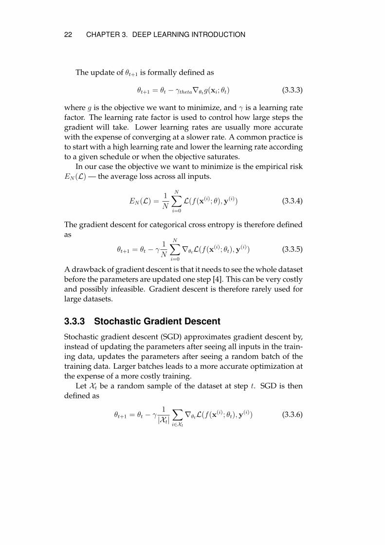
The update of θt+1 is formally defined as
θt+1 = θt − γtheta∇θtg(xi; θt) (3.3.3)
where g is the objective we want to minimize, and γ is a learning ratefactor. The learning rate factor is used to control how large steps thegradient will take. Lower learning rates are usually more accuratewith the expense of converging at a slower rate. A common practice isto start with a high learning rate and lower the learning rate accordingto a given schedule or when the objective saturates.
In our case the objective we want to minimize is the empirical riskEN(L) — the average loss across all inputs.
EN(L) =1
N
N∑i=0
L(f(x(i); θ),y(i)) (3.3.4)
The gradient descent for categorical cross entropy is therefore definedas
θt+1 = θt − γ1
N
N∑i=0
∇θtL(f(x(i); θt),y(i)) (3.3.5)
A drawback of gradient descent is that it needs to see the whole datasetbefore the parameters are updated one step [4]. This can be very costlyand possibly infeasible. Gradient descent is therefore rarely used forlarge datasets.
3.3.3 Stochastic Gradient Descent
Stochastic gradient descent (SGD) approximates gradient descent by,instead of updating the parameters after seeing all inputs in the train-ing data, updates the parameters after seeing a random batch of thetraining data. Larger batches leads to a more accurate optimization atthe expense of a more costly training.
Let Xt be a random sample of the dataset at step t. SGD is thendefined as
θt+1 = θt − γ1
|Xt|∑i∈Xt
∇θtL(f(x(i); θt),y(i)) (3.3.6)

CHAPTER 3. DEEP LEARNING INTRODUCTION 23
Momentum
An extension of SGD is to instead accumulate a velocity vt for each it-eration t of the parameter update, instead of updating the parametersdirectly [54]. At each iteration, the parameters are updated by the ac-cumulated velocity vt. The gradients will have an accelerating effecton the parameters.
SGD with momentum is defined as
vt+1 = µvt − γ1
|Xt|∑i∈Xt
∇θtL(f(x(i); θt),y(i))
θt+1 = θt + vt+1
(3.3.7)
where µ ∈ [0, 1] is the momentum coefficient. The momentum coef-ficient determines how slow the accumulated velocity will decrease.µ = 0 means no momentum is used, and corresponds to the standardSGD.
3.3.4 Weight Decay
Weight decay is a simple way of reducing the risk of over-fitting indeep convolutional networks by adding an extra term in the loss func-tion [26]. Over-fitting can occur when deep convolutional networkslearns complex structures in the training set, while there is actuallylittle information in the training set. Weight decay constraints the net-work by penalizing large weights.
Returning to the standard form of gradient descent in equation3.3.5, the weight decay is formalized as
θt+1 = θt − γ
(1
N
N∑i=0
∇θtL(f(x(i); θt),y(i))− αθt
)(3.3.8)
where α is the weight decay factor. Naturally, the weight decay termcan also be included in SGD and SGD with momentum.
3.3.5 Transfer Learning
Traditional machine learning algorithms assumed that the training andvalidation set for a task are drawn from the same distribution. Thismeans that machine learning models are re-trained from scratch whenfor each new task. However, it has been increasingly more popular to

24 CHAPTER 3. DEEP LEARNING INTRODUCTION
transfer learned parameters from a previous task to a new task. Thisis called transfer learning [39].
This allows knowledge gained from a previous task to be trans-fered to a new task.
It is easy to perform transfer learning on deep convolutional net-works. A common practice is to replace the top layers (often fully con-nected layers) with new, un-trained, layers more suitable for the task[1].
For example, if we have a model trained on a classification problemwith 1000 targets, and we want to use the same model for a classifica-tion problem with 100 targets, we just replace the top fully connectedlayer with a fully connected layer with 100 targets.
For image recognition it is common to use networks pre-trained onlarge datasets such as ImageNet. Some of these are freely available todownload.
Chapter 4
Human Action Recognition
With the basics of deep learning introduced, we can now detail themethods of human action recognition used in this thesis. This chapterwill start by discussing the two-stream convolutional network modelin section 4.1, which is the base-line used for this thesis.
Section 4.2 and 4.3 discusses object detection systems and how toextend object detection systems for human action recognition as a se-mantic stream.
Section 4.4 explores some ideas to jointly train the semantic streamtogether with the spatial and the temporal stream, without changingthe parameters of the latter two streams.
Implementation details are detailed in section 4.5, which discusseshow the streams are trained and evaluated.
4.1 Two-Stream Convolutional Networks
The two-stream convolutional network model, introduced by [50], isone of the most successful approaches to human action recognition invideos. The idea of the two-stream convolutional network is to com-bine the predictions of two separate networks trained on different in-formation.
The first network is trained on the spatial information — raw RGBimages — of the videos. This network is called the spatial stream, andis very similar to image recognition systems. The spatial stream seesonly one frame at a time, so it cannot capture any motion. A way ofinterpreting the spatial stream is that it sees the context of the video.For example, if the action is in a kitchen-like environment, then the
25

26 CHAPTER 4. HUMAN ACTION RECOGNITION
Type Name Filters Kernel Output shapeInput input 3 224× 224
Conv conv1_1 64 3× 3 224× 224
Conv conv1_2 64 3× 3 224× 224
Maxpool pool1 2× 2 112× 112
Conv conv2_1 128 3× 3 112× 112
Conv conv2_2 128 3× 3 112× 112
Maxpool pool2 2× 2 56× 56
Conv conv3_1 256 3× 3 56× 56
Conv conv3_2 256 3× 3 56× 56
Conv conv3_3 256 3× 3 56× 56
Maxpool pool3 2× 2 28× 28
Conv conv4_1 512 3× 3 28× 28
Conv conv4_2 512 3× 3 28× 28
Conv conv4_3 512 3× 3 28× 28
Maxpool pool4 2× 2 14× 14
Conv conv5_1 512 3× 3 14× 14
Conv conv5_2 512 3× 3 14× 14
Conv conv5_3 512 3× 3 14× 14
Maxpool pool5 2× 2 7× 7
FC-4096 fc1 4096FC-4096 fc2 4096FC-1000 fc3 1000Softmax predictions 1000
Table 4.1.1: VGG16 architecture.
action is likely related to cooking.The second network is trained on the temporal information of the
videos. This network is called the temporal stream, and captures themotion of the video. The input of the temporal stream is the opticalflow of multiple consecutive frames of the video.
These two streams provide complementary predictions. Experi-ments show that the average predictions from both streams yield amore accurate prediction than using the streams separately [50].

CHAPTER 4. HUMAN ACTION RECOGNITION 27
4.1.1 VGG16 - A Very Deep Convolutional Network
VGG16 is used as a base for the spatial and the temporal streams,which is a state-of-the-art model for the ImageNet ILSVRC-2012 imagerecognition challenge [51]. It is common to perform transfer learningon VGG16 to other image recognition problems. Pre-trained weightsfrom ImageNet are used as initial weights when training for the hu-man action recognition problem. The architecture of VGG16 is de-picted in table 4.1.1.
4.1.2 Optical Flow
In this section we follow the same notation as used in [50]. The opticalflow is a sequence of displacement vector fields dt. The displacementvector dt(u, v) represents the motion of the point (u, v) between twoconsecutive frames t and t+ 1.
The displacement vector consists of a horizontal vector dxt (u, v) anda vertical vector dy(u, v). The optical flow between two consecutiveframes is therefore W ×H×2, where W and H is the width and heightof the image. It can be seen as a two-channel image where the twochannels represent the horizontal flow and the vertical flow.
The motion across a sequence of frames is represented by stack-ing the flow channels of L consecutive frames. The input is thereforerepresented as a volume of 2L channels.
Mathematically, the input Iτ of a frame τ for the temporal stream isconstructed as follows:
Iτ (u, v, 2k − 1) = dxτ+k−1(u, v),
Iτ (u, v, 2k) = dyτ+k−1(u, v),
u = [1;w], v = [1;h], k = [1;L]
(4.1.1)
We use the precomputed optical flow from [50], which is estimatedwith the TV-L1 optical flow estimation [41].
4.1.3 Spatial Stream
As mentioned earlier, the spatial stream makes a prediction based onthe still RGB frames. The network is based on VGG16 in which the lastlayer is replaced with a fully connected layer with the correct numberof target classes for the dataset. The input of the spatial stream is sub-tracted with the mean of ImageNet.

28 CHAPTER 4. HUMAN ACTION RECOGNITION
4.1.4 Temporal Stream
The temporal stream is also based on VGG16, but with optical flowas input instead of RGB frames. One issue with the temporal streamis that the input uses 2L channels instead of 3 channels for RGB. Toresolve this issue, the first convolutional layer of the temporal streamis replaced with a layer with 2L input channels. We use L = 10 for thetemporal stream, which means the input of the temporal stream is 10consecutive optical flow images.
4.2 Object Detection
Object detection is a more challenging extension of image recognition.While image recognition only consider the presence of a certain targetin an image, object detection also consider the location and size of thetarget. Often there are multiple targets present in the same image forthe object detection system to detect.
4.2.1 YOLO — You Only Look Once
YOLO Introduction
YOLO (You Only Look Once) is a fast and accurate object detectionsystem consisting of one single convolutional network [42]. This meansYOLO proposes bounding boxes and their corresponding class scoressimultaneously.
We use the YOLOv2 and YOLO9000 models. The YOLOv2 trainedon the COCO dataset, which is a dataset for object detection with 80target classes [34]. YOLO9000 on the other hand is trained on Ima-geNet object detection challenge with 200 target classes divided intoover 9000 object categories.
YOLOv2 Architecture
The architecture of YOLOv2 is depicted in table 4.2.1. YOLOv2 mostlyconsists of conventional layers for convolutional neural networks, butthere are a few important notes to point out.
Each convolutional layer is followed by a batch normalization layer.The batch normalization layers are in turn activated by a Leaky ReLU

CHAPTER 4. HUMAN ACTION RECOGNITION 29
# Type Name Filters Kernel Output shape1 Input input 3 224× 224
2 Conv conv1-1 32 3× 3 416× 416
3 Maxpool pool1 2× 2 208× 208
4 Conv conv2-1 64 3× 3 208× 208
5 Maxpool pool2 2× 2 104× 104
6 Conv conv3-1 128 3× 3 104× 104
7 Conv conv3-2 64 1× 1 104× 104
8 Conv conv3-3 128 3× 3 104× 104
9 Maxpool pool3 2× 2 28× 28
10 Conv conv4-1 256 3× 3 52× 52
11 Conv conv4-2 128 1× 1 52× 52
12 Conv conv4-3 256 3× 3 52× 52
13 Maxpool pool4 2× 2 26× 26
14 Conv conv5-1 512 3× 3 26× 26
15 Conv conv5-2 256 1× 1 26× 26
16 Conv conv5-3 512 3× 3 26× 26
17 Conv conv5-4 256 1× 1 26× 26
18 Conv conv5-5 512 3× 3 26× 26
19 Maxpool pool5 2× 2 13× 13
20 Conv conv6-1 1024 3× 3 13× 13
21 Conv conv6-2 512 1× 1 13× 13
22 Conv conv6-3 1024 3× 3 13× 13
23 Conv conv6-4 512 1× 1 13× 13
24 Conv conv6-5 1024 3× 3 13× 13
25 Conv conv6-6 1024 3× 3 13× 13
26 Conv conv6-7 1024 3× 3 13× 13
27 Reorganize conv5-5 to 2048 filters 13× 13
28 Concatenate above with conv6-7 13× 13
29 Conv conv7-1 1024 3× 3 13× 13
30 Conv (Linear) conv7-2 425 1× 1 13× 13
31 Region region 13× 13
Table 4.2.1: The architecture of YOLOv2.

30 CHAPTER 4. HUMAN ACTION RECOGNITION
(see section 3.2.1). The bias of each convolutional layer is also appliedafter the corresponding batch normalization layer.
At layer 24 the channels of ’conv5-3’ output (from layer 16) is stackedon the channels of ’conv6-5’ output (from layer 22). This operation iscalled concatenation. But this operation requires that all channels havethe same shape. This is not the case with ’conv5-3’ and ’conv6-5’. Theshape of ’conv5-3’ is 26× 26, while the shape of ’conv6-5’ is 13× 13.
To solve this the channels of ’conv5-3’ are reorganized at layer 23so that the new shape of ’conv5-3’ is 13 × 13. This means that thenumber of channels of ’conv5-3’ will increase from 512 to 2048. Theconcatenation will therefore have 3062 channels.
The concatenation is then followed by two convolutional layers atlayers 25 and 26 before the regions are predicted at layer 27. The out-put of the network is an array with the shape 13× 13× 425.
YOLO9000 Architecture
The architecture of YOLO9000, depicted in table 4.2.2, is very similarto YOLOv2. The layers are identical between YOLOv2 and YOLO9000up until layer 25, ’conv6-6’. For YOLO9000, ’conv6-6’ is the final con-volutional layer before the region layer. YOLO9000 supports 9418 dif-ferent object categories with 3 predictions for each cell, which is why’conv6-6’ has 28269 output channels (3× (9418 + 5) = 28269).
YOLO Input Format
Unlike VGG16, no mean subtraction is done on the input images ofthe YOLO models. The input of YOLOv2 models are rescaled by thefactor 1/255 instead.
YOLOv2 Output Format
The output of YOLOv2 has fixed size; it is always an array with shape13 × 13 × 425 no matter how many objects are detected. The outputrepresents a 13 × 13 grid of the input image, where each cell of thegrid holds 5 predicted bounding boxes. This means YOLO will alwayspredict 13× 13× 5 = 845 bounding boxes.
Each bounding box holds 4 values for their coordinates in the grid,1 value for the confidence of prediction and a class score vector. Inour case we use YOLOv2 trained on COCO, so the class score vector

CHAPTER 4. HUMAN ACTION RECOGNITION 31
# Type Name Filters Kernel Output shape1 Input input 3 224× 224
2 Conv conv1-1 32 3× 3 416× 416
3 Maxpool pool1 2× 2 208× 208
4 Conv conv2-1 64 3× 3 208× 208
5 Maxpool pool2 2× 2 104× 104
6 Conv conv3-1 128 3× 3 104× 104
7 Conv conv3-2 64 1× 1 104× 104
8 Conv conv3-3 128 3× 3 104× 104
9 Maxpool pool3 2× 2 28× 28
10 Conv conv4-1 256 3× 3 52× 52
11 Conv conv4-2 128 1× 1 52× 52
12 Conv conv4-3 256 3× 3 52× 52
13 Maxpool pool4 2× 2 26× 26
14 Conv conv5-1 512 3× 3 26× 26
15 Conv conv5-2 256 1× 1 26× 26
16 Conv conv5-3 512 3× 3 26× 26
17 Conv conv5-4 256 1× 1 26× 26
18 Conv conv5-5 512 3× 3 26× 26
19 Maxpool pool5 2× 2 13× 13
20 Conv conv6-1 1024 3× 3 13× 13
21 Conv conv6-2 512 1× 1 13× 13
22 Conv conv6-3 1024 3× 3 13× 13
23 Conv conv6-4 512 1× 1 13× 13
24 Conv conv6-5 1024 3× 3 13× 13
25 Conv conv6-6 28269 1× 1 13× 13
26 Region region 13× 13
Table 4.2.2: The architecture of YOLO9000.

32 CHAPTER 4. HUMAN ACTION RECOGNITION
Figure 4.2.1: Illustration of the output of YOLOv2. The image is di-vided into a 13×13 grid. Each cell of the grid holds 5 predicted bound-ing boxes with their corresponding coordinates x, y, w, h, confidence ofprediction c and the class scores.
holds 80 values, one for each class. This means each bounding box isrepresented by a vector of 85 values. The value for confidence is usedto rule out uncertain predictions or background predictions.
Since each cell in the grid holds 5 predictions, each cell holds 85 ×5 = 425 values.
YOLO9000 Output Format
The output format of YOLO9000 is similar to YOLOv2. The only differ-ence is how the class scores are represented. YOLO9000 uses a Word-Net hierarchy for the class scores. WordNet is a language databasewhich models connections between related words in a directed graph[37]. For example, in WordNet, "hunting dog" is a hyponym of "dog".
The class scores of YOLO9000 uses the hyponyms of the class la-bels to model a hierarchy of classes. This allows YOLO9000 to bejointly trained on both COCO and ImageNet. For example, COCO hasthe target class "airplane", while ImageNet has the target classes "jet","biplane", "airbus" and "stealth fighter", all of which are hyponyms of"airplane". Using the hyponym hierarchy, YOLO9000 is able to deducethe relation between "airplane" and "jet".

CHAPTER 4. HUMAN ACTION RECOGNITION 33
4.2.2 SSD — Single Shot MultiBox Detector
SSD (Single Shot Multibox Detector) is an object detection system thatfollows the success of YOLO [35]. In a similar fashion, SSD predictsand classifies the detections in one step. While YOLO and SSD arequite similar in function, there are some notable differences.
Similar to YOLO, SSD is also trained on the COCO dataset. SSD istherefore able to predict 80 different types of object. SSD has also oneclass designated for background. The background class is used to tellthat no object is detected at a particular region. SSD therefore predictsclass scores for 81 different classes for each detection box.
SSD Architecture
SSD has a bit more complicated architecture than YOLO. The outputof SSD involves predictions in many different levels. While YOLOoutputs detection boxes in a 13× 13 grid, SSD outputs detection boxesin grids of various sizes.
The main architecture of SSD is depicted in table 4.2.3. Detectionboxes are predicted from the features of the ’conv4-3’, ’fc7’, ’conv6-2’,’conv7-2’, ’conv8-2’, ’conv9-2’ layers, each representing grids at differ-ent levels for the detection boxes (the grid sizes are 38 × 38, 19 × 19,10× 10, 5× 5 and 3× 3, respectively).
Each cell of the grids holds the bounding boxes and their classscores. The bounding boxes and the class scores are predicted by con-volutional layers connected to each of the mentioned layers. Each con-volutional layer are of kernel size 3 × 3 with 4 × (4 + 81) = 340 filters(4 bounding boxes with 4 values for bounding boxes and 81 classes).
Unlike YOLO, SSD does not perform batch normalization after eachlayer.
SSD Input Format
The input format for SSD is identical as VGG16. The input images aresubtracted by ImageNet mean.
4.3 Semantic Stream
We present the semantic stream, a stream that predicts the humanactions in RGB images depending on the predicted object detections

34 CHAPTER 4. HUMAN ACTION RECOGNITION
Type Name Filters Kernel Strides Output shapeInput input 3 300× 300
Conv conv1-1 64 3× 3 300× 300
Conv conv1-2 64 3× 3 300× 300
Maxpool pool1 2× 2 150× 150
Conv conv2-1 128 3× 3 150× 150
Conv conv2-2 128 3× 3 150× 150
Maxpool pool2 2× 2 2× 2 75× 75
Conv conv3-1 256 3× 3 75× 75
Conv conv3-2 256 3× 3 75× 75
Conv conv3-3 256 3× 3 75× 75
Maxpool pool3 2× 2 2× 2 38× 38
Conv conv4-1 512 3× 3 38× 38
Conv conv4-2 512 3× 3 38× 38
Conv conv4-3 512 3× 3 38× 38
Maxpool pool4 2× 2 2× 2 19× 19
Conv conv5-1 512 3× 3 19× 19
Conv conv5-2 512 3× 3 19× 19
Conv conv5-3 512 3× 3 19× 19
Maxpool pool5 3× 3 1× 1 19× 19
Conv fc6* 1024 3× 3 19× 19
Conv fc7 1024 1× 1 19× 19
Conv conv6-1 256 1× 1 19× 19
Conv conv6-2 512 3× 3 2× 2 10× 10
Conv conv7-1 128 1× 1 10× 10
Conv conv7-2 256 3× 3 2× 2 5× 5
Conv conv8-1 128 1× 1 5× 5
Conv conv8-2 256 3× 3 2× 2 3× 3
Conv conv9-1 128 1× 1 3× 3
Conv conv9-2 128 3× 3 3× 3
Table 4.2.3: SSD main architecture.

CHAPTER 4. HUMAN ACTION RECOGNITION 35
Figure 4.3.1: The semantic stream is divided into two parts: object de-tection and human action recognition. The human action recognitionis based on the predicted object detection features from YOLO/SSD.
from YOLO or SSD. Similar to the spatial stream, the input of the se-mantic stream is one RGB image.
A convenient property with both YOLO and SSD is that the sizeof the output is fixed, no matter how many objects are detected. Thismakes it trivial to extend the models for human action recognition justby adding new layers.
4.3.1 Where to connect YOLO
There are multiple ways of connecting the additional layers of theYOLO network for the semantic stream. The most straightforwardconnection point is the final region layer. Then the input of the se-mantic stream will be the predicted object detections.
An alternative is to connect the semantic stream at earlier layers.The output of earlier layers might hold more information, at the ex-pense of a more complex representation.
For YOLOv2, we consider three different connection points for thesemantic stream, the ’region’ layer, ’conv7-1’ layer and the concatena-tion of the ’conv5-5’ and ’conv6-7’ layers. The reason why we considerthe concatenation of ’conv5-5’ and ’conv6-7’ is that the input of the’conv7-1’ layer uses the output from both of these layers.
For YOLO9000, we consider only one connection point for the se-mantic stream, the ’conv6-5’ layer. Unfortunately, we cannot use the’region’ layer since its output is apparently too large for our equipment(the GPUs became unresponsive after training a few hours).
36 CHAPTER 4. HUMAN ACTION RECOGNITION
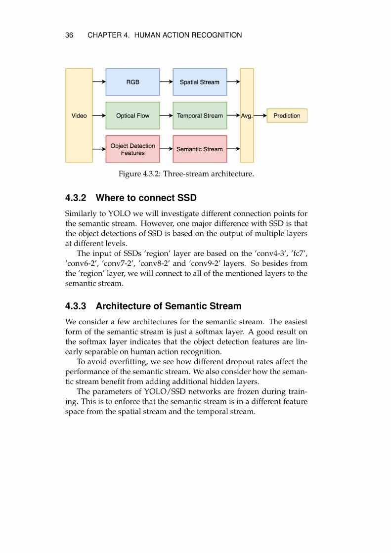
Figure 4.3.2: Three-stream architecture.
4.3.2 Where to connect SSD
Similarly to YOLO we will investigate different connection points forthe semantic stream. However, one major difference with SSD is thatthe object detections of SSD is based on the output of multiple layersat different levels.
The input of SSDs ’region’ layer are based on the ’conv4-3’, ’fc7’,’conv6-2’, ’conv7-2’, ’conv8-2’ and ’conv9-2’ layers. So besides fromthe ’region’ layer, we will connect to all of the mentioned layers to thesemantic stream.
4.3.3 Architecture of Semantic Stream
We consider a few architectures for the semantic stream. The easiestform of the semantic stream is just a softmax layer. A good result onthe softmax layer indicates that the object detection features are lin-early separable on human action recognition.
To avoid overfitting, we see how different dropout rates affect theperformance of the semantic stream. We also consider how the seman-tic stream benefit from adding additional hidden layers.
The parameters of YOLO/SSD networks are frozen during train-ing. This is to enforce that the semantic stream is in a different featurespace from the spatial stream and the temporal stream.

CHAPTER 4. HUMAN ACTION RECOGNITION 37
4.3.4 Fusion of Streams
In [14] a few functions for fusing the spatial and the temporal streamwere investigated at different fusion layers. It was concluded that thesum of the softmax layers is the most efficient approach. We followthis conclusion and fuse the three streams by summing their softmaxlayers.
4.4 Boosting Divergence
The ultimate goal with the semantic stream is that it will provide com-plementary information to the spatial and the temporal streams. Thesemantic stream does not necessarily need to perform well on its own.It is more important that it makes different kinds of error to the spatialand the temporal stream.
We will therefore investigate a few ways to enforce the predictionsdiverge from each other.
Generating new models to be complementary to other models isnot new. The most well-known example is AdaBoost [16], a boost-ing technique for weak classifiers. AdaBoost iteratively generates newmodels focused to complement the previous iterations of the model.
For speech recognition [5] investigated Minimum Bayes Risk Lever-aging for training complementary models. The technique successfullycreated complementary models and reduced the error rates comparedto individually trained models.
We will investigate some alternative techniques to boost the diver-gence between the streams. These techniques only adds a new term tothe loss function.
4.4.1 Average Layer
Possibly the most trivial approach is to train the semantic stream jointlytogether with the spatial and the temporal stream.
Laverage(ysem,y) = Lcross(w0ysem + w1yspa + w2ytem
w0 + w1 + w2
,y
)(4.4.1)
The weights w0, w1 and w2 are used weight the average of the streams.The spatial and the temporal stream both perform too well on thetraining set and thus overshadow the predictions of the semantic stream.

38 CHAPTER 4. HUMAN ACTION RECOGNITION
We therefore set w0 = 1 and w1 = w2 = 0.25. This gives the semanticstream more influence, even if the predictions of the spatial and thetemporal stream are too confident on the true value.
The idea with this technique is to simulate the validation of themodel. The semantic stream can focus to be less correct in the caseswhere both the spatial and the temporal stream are confident on thetrue value, and focus to be more correct in the cases where the spatialand temporal stream are not confident.
4.4.2 Kullback-Leibler Divergence
Another approach is to use a divergence measurement to enforce di-vergence between the predicted streams. One popular divergence mea-surement for probability distributions is the Kullback-Leibler diver-gence KL [28], defined for discrete probability distributions as
KL(p||q) =∑i
pi logpiqi
(4.4.2)
where p and q are two discrete probability distributions (of the samesize). KL(p||q) is grows as p and q diverges, and KL(p||q) = 0 whenp = q. Note that KL(p||q) 6= KL(q||p).
We define the loss function LKL as
LKL(ysem,y) = Lcross(ysem,y)− λKLKL(
ysem,yspa + ytem
2
)(4.4.3)
where λKL is a scaling factor controlling how much the Kullback-Leiblerdivergence influences the loss.
4.4.3 Dot Product Divergence
A more geometric approach is to minimize the dot product betweenthe predicted distributions. If the predictions are viewed in a vectorspace, the dot-product is minimized when the vectors are orthogonal.A geometric interpretation is that two probabilities are divergent whentheir angle is as large in the probability distribution vector space. Wedefine the loss function Ldot
Ldot(ysem,y) = Lcross(ysem,y) + λdotysem · (yspa + ytem) (4.4.4)
where λdot is a scaling factor controlling how much the dot productinfluences the loss.

CHAPTER 4. HUMAN ACTION RECOGNITION 39
4.4.4 Combining Average with Divergence
We also consider two mixtures of the above techniques — for Ldotand LKL, we replace Lcross with Laverage. We define Laverage+dot andLaverage+KL as
Laverage+dot(ysem,y) =Laverage(ysem,y)
+λdotysem · (yspa + ytem) (4.4.5)
and
Laverage+KL(ysem,y) =Laverage(ysem,y)
−λKLKL(
ysem,yspa + ytem
2
)(4.4.6)
4.5 Implementation Details
4.5.1 Training
Sampling
The models are trained in a similar procedure as described in [14]. Theclips are uniformly sampled across the clip categories. From each sam-pled clip a single frame is randomly selected uniformly. The singleframe is randomly cropped and horizontally flipped.
For training the temporal stream we uniformly sample L consecu-tive frames of the precomputed optical flow of the clip. The sequenceof the optical flows is spatially randomly cropped and horizontallyflipped.
Batch Size
We use a batch size of 64 for all experiments. When training the spatialand the temporal spatial stream we divide the batch across two GPUs.The weights for each iteration is updated with the average gradient ofthe batches across the multiple GPUs. For the semantic stream we useonly one GPU.
Epochs
The training is divided into epochs. One epoch corresponds to 100 it-erations of SGD parameter update. After each epoch the average vali-

40 CHAPTER 4. HUMAN ACTION RECOGNITION
dation loss is computed on 12,800 inputs randomly sampled from thevalidation set.
Learning Rate Decay
The learning rate is decreased by a factor of 0.1 if the validation losshas not decreased for 3 epochs. The training is terminated when thevalidation loss has not been decreased for more than 10 epochs. A finalevaluation on a clip basis is made with the model with the lowest vali-dation loss (see section 4.5.3). Unless mentioned, the starting learningrate is 5× 10⁻³.
Weight Decay
The weight decay is set to 5× 10⁻³ for the weight parameters, and 0.0for the bias parameters for all trained models.
4.5.2 Datasets
We use two datasets for human action recognition, UCF-101 and HMDB-51. These two are currently the most common sets for human actionrecognition.
We use the pre-computed optical flow of UCF-101 and HMDB-51provided by [14].
UCF-101
UCF-101 is a collection of 13320 clips downloaded from from YouTubewith a total of 27 hours of video data. The clips are typically in uncon-strained environments. With varying lighting, camera motion, partialocclusion and low quality frames makes the dataset challenging andrealistic [52].
The clips are labeled with 101 different action categories. The ac-tions are according to the authors divided into five different types: 1)Human-object interaction; 2) Body-motion only; 3) Human-human in-teraction; 4) Playing musical instruments; 5) Sports. However, there isno additional labeling for these five types. The different action cate-gories are depicted in table A.2.1.
Each action class is divided into 25 different groups, where eachgroup consist of 4-7 clips. The clips in each group share common fea-tures such as actors and sceneries. Typically the groups represent clips

CHAPTER 4. HUMAN ACTION RECOGNITION 41
from the same video. There are 3 training/validation splits for UCF-101.
HMDB-51
Human Motion Database (HMDB-51) is another dataset for human ac-tion recognition proven to be more challenging than UCF-101. HMDB-51 consists 6,766 videos labeled with 51 different action categories,which are depicted in table A.1.1 [27]. Each category consists of atleast 101 clips.
The actions are according to the authors divided into five types:1) General facial actions; 2) Facial actions with object manipulation; 3)General body movements; 4) Body movements with object interaction;5) Body movements with human interaction.
The videos are collected from digitized movies, public databases,YouTube, Google Videos and other videos collected from the internet.
4.5.3 Evaluation
We follow the same evaluation protocol as used in [50]. For each clip,we sample 25 frames with spaced equally temporally. For each frame,we crop 5 different regions: one in each corner and one in the center.We also flip each of the crops so we get in total 10 different inputs foreach frame. In total, each stream makes 250 different predictions foreach clip.
The class scores for the clip is then obtained by averaging the pre-dictions of the sampled crops.
4.5.4 Equipment
We use Keras 2.0 [7] with Tensorflow backend [9] for the implementa-tion, training and evaluation of the models. GeForce GTX 1080 GPUsare used for our experiments.
Our SSD implementation is based on the Keras port by [47]. Weported the YOLO weights from its original implementation in Darknetto Keras [43]. The weights of the spatial and the temporal streams forUCF-101 are ported from its original implementation in MatConvNetto Keras [14]. For HMDB-51 we needed to train the spatial and thetemporal stream by ourselves.

Chapter 5
Results
Our experimental results are reported in this chapter. First in section5.1 we set up the spatial and the temporal stream in our working en-vironment to match the results reported in [14] as closely as possible.
Section 5.2 explores the possibilities to predict human actions withobject detections by investigating which kind of objects are detected infor different human actions.
Section 5.3 finally investigates different architectures for the seman-tic stream. Initially we perform all experiments on UCF-101 split 1.The most promising models will be then used for the remainder of theUCF-101 splits and all of the HMDB-51 splits.
5.1 Setting up the Spatial and the TemporalStreams
Present the results from our trained VGG16 models. Discuss brieflywhy there might be some differences. Better results were reported in[61] if the temporal stream is counted twice as much as the spatialstream. We do the same for our own experiments.
We use the same weights as twostream fusion paper for the modelstrained on the UCF-101 dataset. The weights are converted to Keras2.0 with Tensorflow backend. The original weights were trained withMatConvNet.
Unfortunately there are no publicly available weights for the spa-tial and the temporal stream pre-trained on the HMDB-51 dataset. Wehave to train the weights for HMDB-51 by ourselves. This is done by
42

CHAPTER 5. RESULTS 43
S T S + T S + 2TOurs UCF-101 split 1 82.79% 86.44% 89.90% 90.96%Ours HMDB-51 split 1 40.6% 50.45% 54.83% 56.21%
Table 5.1.1: Differences between the reported accuracy of the streamsin [14] and the observed accuracy with our implementation.
fine-tuning the pre-trained weights from UCF-101. We compare theweights reported from [14] with our implementation in table 5.1.1.
Our scores a bit off from the scores reported by [14]. It is unknownwhy the results are worse. A possible cause can be slight implemen-tation differences between Keras/Tensorflow and MatConvNet. An-other possible cause can be slight differences in the evaluation scheme.
5.2 Objects Detected in Clips
To get a better idea of how effective YOLO and SSD can detect theactions in the clips, we determine the top 10 most detected objects foreach action. A great diversity of objects between the actions indicatesthat most of the information of the action is maintained through thenetwork.
This is done by sampling 25 frames with equal temporal spacingfrom each clip. For each frame we compute the final prediction layerof YOLO and SSD. For each detection box we compute a certainty vec-tor by multiplying the predicted probability vector with the certaintyscalar. Each certainty vector is then summed across all detection boxesfor each action.
To express it more mathematically, let Ci be the number of clipsof action class i, D be the number of detection boxes generated foreach frame, cic,f,d and pic,f,d the certainty scalar and probability vectorof detection box d in frame f in clip c of action i. Then we have thetotal certainty citot for action i defined as
citot =
Ci∑c=0
25∑f=0
D∑d=0
cic,f,d · pic,f,d (5.2.1)
We then take the top 10 largest values of each citot. Figures 5.2.1 presentthe object detection matrices.

44 CHAPTER 5. RESULTS
We can see YOLO detects a more diverse set of objects than SSD inboth UCF-101 and HMDB-51.
We believe this is due to that SSD is trained with a special targetclass for backgrounds. Uncertain predictions might be concentratedon the background class. YOLO will always try to predict the targetclass, even if it is uncertain about the prediction.
5.3 Experiments
5.3.1 Where to Connect the Semantic Stream
We now investigate how well the different object detection systemsrepresents the human actions by connecting a softmax layer to differ-ent layers of the object detection systems (as described in sections 4.3.1and 4.3.2). This experiment will show how linearly separable the fea-tures for object detection are for the action recognition problem.
The initial learning rate for YOLOv2 and SSD is set to 0.0005. YOLO9000requires an initial learning rate as low as 0.000005. The loss divergesfor higher learning rates.
The results are presented in table 5.3.1. Individually, YOLO9000yields the most accurate prediction. Together with the spatial andthe temporal streams, YOLOv2 is consequently more accurate thanYOLO9000. Overall, the ’conv7-1’ layer of YOLOv2 yields the bestresults when the semantic stream predictions are combined with onespatial stream and two spatial streams.
SSD on the other hand yields the poorest results. This indicates thatthe architecture of YOLO is the best feature representation for humanaction recognition.
For our continued experiments the semantic stream is connected tothe ’conv7-1’ layer of YOLOv2.
5.3.2 Dropout Rates
In this subsection we attempt to improve the generality of the semanticstream by using dropout on its output. The affect of different dropoutrates is presented in table 5.3.2.
1O: Semantic stream (with Object detections)

CHAPTER 5. RESULTS 45
(a) YOLO training set. (b) YOLO validation set.
(c) SSD training set. (d) SSD validation set.
Figure 5.2.1: Top 10 detections on UCF-101 split 1. Darker squaresrepresent larger representation of the detection class.

46 CHAPTER 5. RESULTS
(a) YOLO training set. (b) YOLO validation set.
(c) SSD training set. (d) SSD validation set.
Figure 5.2.2: Top 10 detections on HMDB-51 split 1. Darker squaresrepresent larger representation of the detection class.
Connection Point O1 O+S O+T O+S+T O+S+2TYOLOv2 ’region’ 55.09% 82.58% 87.79% 89.51% 90.77%
’conv7-1’ 70.95% 82.84% 88.90% 89.24% 90.80%’conv6-7’ + ’conv5-5’ 71.85% 82.95% 88.82% 89.24% 90.75%
YOLO9000 ’conv6-5’ 73.83% 82.47% 88.82% 89.00% 90.72%SSD ’region’ 45.15% 82.45% 85.94% 89.40% 90.48%
multiple 42.85% 79.94% 82.66% 88.47% 89.35%
Table 5.3.1: Results from UCF-101 split 1 by connecting a softmax layerto different layers.

CHAPTER 5. RESULTS 47
Rate O O+S O+T O+S+T O+S+2T0% 70.95% 82.84% 88.90% 89.24% 90.80%
10% 72.96% 83.06% 88.63% 89.59% 90.80%25% 72.40% 83.32% 88.74% 89.27% 90.80%50% 72.59% 83.32% 89.03% 89.61% 91.14%75% 72.05% 82.82% 88.61% 89.43% 90.83%90% 69.83% 82.13% 87.07% 88.58% 90.40%
Table 5.3.2: The effect of different dropout rates for YOLOv2 with’conv7-1’ as connection point for the semantic stream (UCF-101 split1).
Individually, the semantic stream performs best with dropout rate25%. Together with the other two streams, dropout rate 50% conse-quently outperforms other dropout rates.
5.3.3 Adding Additional Hidden Layers
We explore different architectures for the semantic stream by addingadditional hidden layers. Five different architectures are considered.All hidden convolutional and fully connected layers are activated withReLU.
1. softmax: No hidden layers are used. The model is a dropoutlayer with dropout rate 50% followed by a softmax layer. Thesame as the best architecture in section 5.3.2.
2. fc1024: Fully connected layer with 1024 nodes is used as a hiddenlayer. The fully connected layer is followed by a dropout layerwith dropout rate 50% and a softmax layer.
3. 2×fc1024: Two fully connected layers with 1024 are used as hid-den layers. A dropout layer with dropout rate 50% is used be-tween the two fully connected layers. The hidden layers are fol-lowed by a dropout layer with dropout rate 50% and a softmaxlayer.
4. convolution: One 3× 3 convolutional layer with 1024 filters, one2× 2 max pooling layer and one fully connected layer with 4096

48 CHAPTER 5. RESULTS
Hidden Layers O O + S O + T O + S + T O + S + 2Tsoftmax 72.59% 83.32% 89.03% 89.61% 91.14%
fc1024 73.04% 83.21% 88.68% 89.11% 90.80%2×fc1024 70.82% 82.90% 88.95% 89.32% 90.80%
convolution 72.98% 83.18% 89.05% 89.43% 90.83%2×convolution 73.72% 83.48% 88.95% 89.72% 90.98%
Table 5.3.3: The effect of different architectures for YOLOv2 with’conv7-1’ as connection point for the semantic stream (UCF-101 split1).
nodes. The hidden layers are followed by a dropout layer withdropout rate 50% and a softmax layer.
5. 2xconvolution: One 3 × 3 convolutional layer with 1024 filters,one 2×2 max pooling layer, another 3×3 convolutional layer butwith 2048 filters, another 2 × 2 max pooling layer and one fullyconnected layer with 4096 nodes. The hidden layers are followedby a dropout layer with dropout rate 50% and a softmax layer.
The results in table 5.3.3 shows that hidden layers gives small im-provements in the if the semantic stream is used individually and inthe O + S, O + T and O + S + T settings. Using no hidden layers is bestfor the O + S + 2T setting.
5.3.4 Divergence Boosting
We explore how the different divergence boosting methods from sec-tion 4.4 affects the training. We initialize the models with the weightstrained for YOLOv2 with dropout rate 50% trained in section 5.3.2.The configurations we consider are
1. average: The categorical cross entropy is replaced with the aver-age layer as described in section 4.4.1.
2. dot 0.1: The dot product divergence as described in section 4.4.3with λdot = 0.1.
3. dot 0.5: The dot product divergence as described in section 4.4.3with λdot = 0.5.

CHAPTER 5. RESULTS 49
Divergence Boost O O + S O + T O + S + T O + S + 2Tno divergence boost 72.59% 82.32% 89.03% 89.61% 91.14%
average 71.72% 82.87% 88.63% 89.45% 90.80%dot 0.1 72.59% 83.21% 88.98% 89.74% 91.22%dot 0.5 72.48% 83.27% 88.95% 89.80% 91.28%
KL 0.005 73.46% 83.29% 89.03% 89.37% 91.01%KL 0.01 73.51% 83.03% 89.03% 89.56% 90.99%
average + dot 0.1 72.53% 83.19% 88.69% 89.58% 90.91%average + dot 0.5 68.01% 82.32% 88.08% 89.37% 91.20%
average + KL 0.005 72.24% 82.98% 88.87% 89.43% 91.07%average + KL 0.01 71.98% 83.14% 88.50% 89.53% 90.85%
Table 5.3.4: The effect of the different divergence boosting methodson UCF-101 split 1. YOLOv2 with ’conv7-1’ as connection point anddropout rate 50% is used.
4. KL 0.005: The Kullback-Leibler divergence as described in sec-tion 4.4.2 with λKL = 0.005.
5. KL 0.01: The Kullback-Leibler divergence as described in section4.4.2 with λKL = 0.01.
Besides from the above listed configurations, we also consider acombination with the average layer together with the dot product di-vergence and the Kullback Leibler divergence as described in section4.4.4. The same values of λdot and λKL is used as above.
The results in table 5.3.4 shows that dot product divergence withλdot = 0.5 is the most effective on the O + S + 2T setting.
5.3.5 Experiments on HMDB-51
We now investigate how well the most promising models on UCF-101 performs on HMDB-51. Four models for the semantic stream areinvestigated.
1. YOLOv2 conv7-1: A softmax layer directly connected to the ’conv7-1’ layer of YOLOv2.
2. Dropout 50%: Same as above, but with a dropout layer addedbetween ’conv7-1’ and the softmax layer.

50 CHAPTER 5. RESULTS
Experiment O O + S O + T O + S + T O + S + 2TYOLOv2 conv7-1 42.68% 45.62% 54.97% 54.44% 57.25%
Dropout 50% 43.86% 45.49% 54.57% 53.79% 57.32%Dot 0.5 43.46% 46.80% 53.99% 53.92% 56.41%KL 0.01 43.99% 45.82% 53.52% 53.59% 56.01%
Table 5.3.5: Different models on the HMDB-51 dataset split 1.
3. Dot 0.5: Same as above, but trained with dot product divergenceas described in section 4.4.3 with λdot = 0.5.
4. KL 0.001: Same as 2, but trained with Kullback-Leibler diver-gence as described in section 4.4.2 with λKL = 0.001.
The results in table 5.3.5 indicate that using dot product divergenceis not as effective as in UCF-101. Instead, only using a dropout layer50% seem to be most effective. We can also observe that as in UCF-101,KL 0.001 gives slight improvements to the semantic stream individu-ally.
5.3.6 Mean Accuracy over all Three Splits
Finally we evaluate the following three models over all three splits onUCF-101 and HMDB-51: ’YOLOv2 conv7-1’, ’Dropout 50%’ and ’Dot0.5’. The results are depicted in table 5.3.6.
5.3.7 Per Class Accuracy
We now study which actions perform well under the semantic stream,and which that does not. We use YOlOv2 ’conv7-1’ with dropout 50%as a semantic stream for the following experiments. Figure 5.3.1 de-picts the recall rate of the semantic stream. We see that the semanticstream perfectly recognizes the classes ’Cutting in kitchen’, ’Surfing’,’Knitting’, ’Writing on board’, ’Billiards’, ’Playing dhol’ ’Playing tabla’,’Fencing’, ’Basketball’, ’Diving’, ’Horse riding’, ’Drumming’, ’Volley-ball spiking’, ’Baby crawling’ and ’Breaststroke’.
The three worst recognized classes are in order ’Jumping jack’, ’Nunchucks’and ’Boxing punching bag’. ’Jumping jack’ contains in general nohuman-object interaction, so it is understandable that the semantic

CHAPTER 5. RESULTS 51
Experiment O O+S O+T O+S+T O+S+2TYOLOv2 conv7-1UCF-101 Split 1 70.95% 82.84% 88.90% 89.24% 90.80%UCF-101 Split 2 65.91% 80.02% 88.51% 88.16% 90.17%UCF-101 Split 3 70.31% 81.85% 90.77% 89.29% 92.18%UCF-101 Split Average 69.06% 81.57% 89.39% 88.90% 91.05%HMDB-51 Split 1 42.68% 45.62% 54.97% 54.44% 57.25%HMDB-51 Split 2 36.93% 43.01% 52.48% 50.52% 54.11%HMDB-51 Split 3 39.09% 42.35% 52.16% 50.91% 54.77%HMDB-51 Split Average 39.57% 43.66% 53.20% 51.96% 55.38%Dropout 50%UCF-101 Split 1 72.59% 83.32% 89.03% 89.61% 91.14%UCF-101 Split 2 71.00% 80.24% 88.00% 87.60% 90.23%UCF-101 Split 3 70.81% 81.95% 89.61% 89.12% 92.10%UCF-101 Split Average 71.47% 81.84% 88.88% 88.78% 91.16%HMDB-51 Split 1 43.86% 45.49% 54.57% 53.79% 57.32%HMDB-51 Split 2 38.43% 42.94% 50.33% 50.59% 54.18%HMDB-51 Split 3 39.15% 42.42% 51.31% 51.05% 54.90%HMDB-51 Split Average 40.48% 43.62% 52.07% 51.81% 55.47%Dot 0.5UCF-101 Split 1 72.48% 83.27% 88.95% 89.80% 91.28%UCF-101 Split 2 72.36% 80.29% 88.46% 87.81% 90.28%UCF-101 Split 3 71.94% 81.93% 90.21% 89.29% 91.94%UCF-101 Split Average 72.26% 81.83% 89.21% 88.97% 91.17%HMDB-51 Split 1 43.46% 46.80% 53.99% 53.92% 56.41%HMDB-51 Split 2 39.02% 42.94% 50.33% 51.18% 53.99%HMDB-51 Split 3 38.43% 41.57% 50.98% 50.39% 54.64%HMDB-51 Split Average 40.30% 43.77% 51.77% 51.83% 55.01%
Table 5.3.6: Collective results over all datasets and splits.

52 CHAPTER 5. RESULTS
stream has difficulties to recognize the action. ’Nunchucks’ is an human-object interaction, which should be an action the semantic stream shouldbe good at classifying. However, there are no nunchuck representedin the COCO dataset, which might cause some confusion. ’Boxingpunching bag’ is in general mixed up with ’Boxing speed bag’ as canbe seen in the confusion matrix in figure 5.3.2.
The results on HMDB-51 are evidently worse. Two actions werenever correctly recognized: ’Smile’ and ’Ride bike’. It is not surpris-ing that ’Smile’ is difficult to recognize for the semantic stream — thesemantic stream is unable to capture facial expressions. However, itis quite surprising that ’Ride bike’ is difficult to recognize, especiallysince ’Bicycle’ is in the COCO dataset. YOLO is also able to recog-nize bicycles in the ’Ride bike’ actions of HMDB-51 according to thedetection matrix in figure 5.2.2.
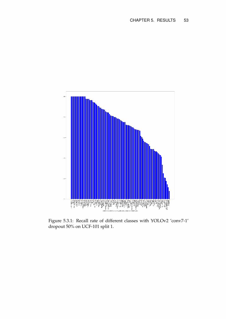
CHAPTER 5. RESULTS 53
Figure 5.3.1: Recall rate of different classes with YOLOv2 ’conv7-1’dropout 50% on UCF-101 split 1.

54 CHAPTER 5. RESULTS
Figure 5.3.2: Confusion matrix with YOLOv2 ’conv7-1’ dropout 50%on UCF-101 split 1.

CHAPTER 5. RESULTS 55
Figure 5.3.3: Recall rate of different classes with YOLOv2 ’conv7-1’dropout 50% on HMDB-51 split 1.
Figure 5.3.4: Confusion matrix with YOLOv2 ’conv7-1’ dropout 50%on HMDB-51 split 1.

Chapter 6
Discussion
Overall our experiments indicates that the semantic stream achieves asmall improvement to the two-stream convolutional network. We be-lieve the results could potentially be further improved if more accuratearchitectures are used.
A potential drawback of the semantic stream is its inaccuracy whenused individually.
6.1 Comparison of Object Detection Systems
Our experiments indicates that SSD is not suitable for predicting actionrecognition. A possible cause is that SSD will predict a region as abackground if all of other object categories are unlikely. Importantinformation for action recognition purposes might be filtered out bythis behavior.
The YOLO models might be better in this case because a predic-tion is always made, even if the prediction is uncertain. For example,YOLO might incorrectly detect a certain object as a cat. This certain ob-ject might not be included in the COCO dataset. The semantic streamcould without loss of performance associate the action with the ap-pearance of a cat — even if no cat actually appears in the videos.
6.2 Comparison with State-of-the-Art
Our results does not break the current state-of-the-art in human ac-tion recognition, but is comparable at least for UCF-101 (table 6.2.1.
56

CHAPTER 6. DISCUSSION 57
Method UCF-101 HMDB-51Two-Stream [50] 88.0% 59.4%Two-Stream [14] 91.7% 58.7%Two-Stream Fusion [14] 92.5% 65.4%Temporal Segment Networks [59] 94.2% 69.4%Chained Multi-Stream Networks [63] 91.1% 69.7%Key Volume Mining Framework [62] 93.1% 63.3%Ours (Dropout 50%) 91.16% 55.47%Ours (Dot 0.5) 91.17% 55.01%
Table 6.2.1: Mean classification accuracy over three splits in some cur-rent state of the art methods.
A reason why HMDB-51 is very low compared to the state-of-the-artis because our spatial and temporal streams are inaccurate. It is un-known why our spatial and temporal streams does not perform wellon HMDB-51, while the streams perform well on UCF-101. We expectthe result to be higher if we manage to train the spatial and the tempo-ral stream to the same levels as [14].
6.3 Directions of Improvement
We believe there is much room for improvement. Due to time con-straints we were not able to fully investigate the proposed models andtechniques in this thesis. We suggest a few interesting directions tofurther improve our work.
6.3.1 Temporal Setting
We only applied the semantic stream on a single-frame basis. Furtherprogress can be made if the semantic stream predictions are made on amulti-frame basis in a temporal setting. This would allow the semanticstream to capture the evolution of the object detections over a sequenceof frames.
A potential challenge with the temporal setting is to correctly as-sociate the object detections between the frames. We are not sure howimportant this issue may be. It is possible that the semantic stream isable to learn the associations by itself.
58 CHAPTER 6. DISCUSSION
6.3.2 Very Deep Semantic Streams
Our semantic streams were rather shallow. At most three hidden lay-ers were used in our experiments. A potential improvement is toconstruct even deeper networks for the semantic stream. Our experi-ments indicated small improvements in some cases when using hid-den layers. The very deep networks can be fine tuned using pre-trained weights learned from large-scale datasets like ImageNet.
6.3.3 Further Investigations on Divergence Boosting
The divergence boosting had little effect on the semantic stream, butthe results are still promising. Interestingly, the accuracy of the seman-tic streams were not decreased significantly after training with diver-gence boost. In some cases the semantic streams even became moreaccurate.
Our initial intention with the divergence boost was that the seman-tic stream would sacrifice some of its accuracy in order to boost theaccuracy in a three-stream case. This does not seem to be the case ex-cept for the ’average + dot 0.5’ configuration.
Interestingly the dot product divergence did not have any positiveeffect on HMDB-51. A possible cause for this is the inaccuracy of thespatial and the temporal stream on the dataset. A deeper investiga-tion is required to determine when dot product divergence works, andwhen it does not.
But possibly most interestingly is how the Kullback-Leibler diver-gence improved the models on an individual basis. This raises thequestion if this is always the case, and if the Kullback-Leibler diver-gence can be used to further boost trained models.
The methods for divergence boosting presented here is still in itsinfancy, and we believe further investigations can be interesting. Forexample, the spatial and the temporal streams can also be trained withthe divergence boosting techniques. The spatial and the temporal streamsare both very accurate already. It would be interesting to investigatehow divergence boosting affects models which are already accurate.
The divergence boosting is also applied on data which are alreadyseen by the models. We did not have any unseen data available for ourexperiments. Training with divergence boosting on already seen datacan give skewed results since the spatial and the temporal streams are

CHAPTER 6. DISCUSSION 59
both very accurate on the training set. This is a possible cause of whythe average layer performed poorly.
6.3.4 More Object Categories
One major drawback of the object detection systems used in this the-sis is that the object categories in COCO is not very representative ofthe human actions in UCF-101 and HMDB-51. For example, COCOhas the object categories elephant and teddy bear, but no hammer ornunchucks. Some important object categories for certain actions inUCF-101 and HMDB-51 are missing from the COCO dataset.
YOLO9000 partially resolves this issue by being trained on mul-tiple datasets and able to determine the relation between categoriesthanks to word-net. However, YOLO9000 is only trained on a subsetof the object categories it is capable of detecting.
Object detection for human action recognition could probably beimproved once it is possible to train object detection systems to recog-nize a very large number of object categories.

Chapter 7
Conclusion
From our work we can conclude slight improvements when using ob-ject detections for human action recognition. We have compared threedifferent one-pass object detection systems. YOLOv2 and YOLO9000both seem promising for human action recognition. SSD on the otherhand is not a very good feature representation of human actions.
Different architectures of the semantic stream were tried. Non-linear models did not provide a big overhead over linear models whenthe semantic stream is used together with the spatial and the temporalstreams.
Our divergence boosting techniques gave slight improvements. TheKullback-Leibler even had the effect of improving the semantic streamon an individual basis.
We believe we have not reached the full potential of the seman-tic stream. Deeper networks pre-trained on ImageNet and predictingin a temporal setting are some potential directions to bring the workfurther. There is definitely room for more work to fully develop thesemantic stream.
60

Bibliography
[1] Hossein Azizpour, Ali Sharif Razavian, Josephine Sullivan, At-suto Maki, and Stefan Carlsson. “Factors of transferability for ageneric convnet representation”. In: IEEE Transactions on PatternAnalysis and Machine Intelligence 38.9 (2016), pp. 1790–1802.
[2] Peter N. Belhumeur, João P Hespanha, and David J. Kriegman.“Eigenfaces vs. fisherfaces: Recognition using class specific lin-ear projection”. In: IEEE Transactions on pattern analysis and ma-chine intelligence 19.7 (1997), pp. 711–720.
[3] Moshe Blank, Lena Gorelick, Eli Shechtman, Michal Irani, andRonen Basri. “Actions as space-time shapes”. In: Computer Vi-sion, 2005. ICCV 2005. Tenth IEEE International Conference on. Vol. 2.IEEE. 2005, pp. 1395–1402.
[4] Léon Bottou. “Large-scale machine learning with stochastic gra-dient descent”. In: Proceedings of COMPSTAT’2010. Springer, 2010,pp. 177–186.
[5] Catherine Breslin and Mark JF Gales. “Generating complemen-tary systems for speech recognition.” In: INTERSPEECH. 2006.
[6] Zezhou Cheng, Qingxiong Yang, and Bin Sheng. “Deep coloriza-tion”. In: Proceedings of the IEEE International Conference on Com-puter Vision. 2015, pp. 415–423.
[7] François Chollet. Keras. https://github.com/fchollet/keras. 2015.
[8] Convolutional Neural Networks. http://cs231n.github.io/convolutional-networks/. Accessed: 2017-05-19.
[9] Jeffrey Dean and Rajat Monga. “TensorFlow: Large-Scale Ma-chine Learning on Heterogeneous Distributed Systems”. In: GoogleResearch Whitepaper, http://research.google.com/pubs/archive/45166.pdf (2015).
61

62 BIBLIOGRAPHY
[10] Jia Deng, Wei Dong, Richard Socher, Li-Jia Li, Kai Li, and Li Fei-Fei. “Imagenet: A large-scale hierarchical image database”. In:Computer Vision and Pattern Recognition, 2009. CVPR 2009. IEEEConference on. IEEE. 2009, pp. 248–255.
[11] Li Deng, Dong Yu, et al. “Deep learning: methods and appli-cations”. In: Foundations and Trends R© in Signal Processing 7.3–4(2014), pp. 199–200.
[12] Oscar Déniz, Gloria Bueno, Jesús Salido, and Fernando De laTorre. “Face recognition using histograms of oriented gradients”.In: Pattern Recognition Letters 32.12 (2011), pp. 1598–1603.
[13] Jeffrey Donahue, Lisa Anne Hendricks, Sergio Guadarrama, Mar-cus Rohrbach, Subhashini Venugopalan, Kate Saenko, and TrevorDarrell. “Long-term recurrent convolutional networks for visualrecognition and description”. In: Proceedings of the IEEE confer-ence on computer vision and pattern recognition. 2015, pp. 2625–2634.
[14] Christoph Feichtenhofer, Axel Pinz, and Andrew Zisserman. “Con-volutional two-stream network fusion for video action recogni-tion”. In: Proceedings of the IEEE Conference on Computer Vision andPattern Recognition. 2016, pp. 1933–1941.
[15] Pedro F Felzenszwalb, Ross B Girshick, David McAllester, andDeva Ramanan. “Object detection with discriminatively trainedpart-based models”. In: IEEE transactions on pattern analysis andmachine intelligence 32.9 (2010), pp. 1627–1645.
[16] Yoav Freund and Robert E Schapire. “A desicion-theoretic gen-eralization of on-line learning and an application to boosting”.In: European conference on computational learning theory. Springer.1995, pp. 23–37.
[17] Georgia Gkioxari, Ross Girshick, and Jitendra Malik. “Contex-tual action recognition with r* cnn”. In: Proceedings of the IEEEinternational conference on computer vision. 2015, pp. 1080–1088.
[18] Xavier Glorot, Antoine Bordes, and Yoshua Bengio. “Deep SparseRectifier Neural Networks.” In: Aistats. Vol. 15. 106. 2011, p. 275.
[19] Ian Goodfellow, Yoshua Bengio, and Aaron Courville. Deep Learn-ing. http://www.deeplearningbook.org. MIT Press, 2016,pp. 371–372.

BIBLIOGRAPHY 63
[20] Alex Graves and Navdeep Jaitly. “Towards End-To-End SpeechRecognition with Recurrent Neural Networks.” In: ICML. Vol. 14.2014, pp. 1764–1772.
[21] Sergey Ioffe and Christian Szegedy. “Batch normalization: Ac-celerating deep network training by reducing internal covariateshift”. In: arXiv preprint arXiv:1502.03167 (2015).
[22] Shuiwang Ji, Wei Xu, Ming Yang, and Kai Yu. “3D convolutionalneural networks for human action recognition”. In: IEEE transac-tions on pattern analysis and machine intelligence 35.1 (2013), pp. 221–231.
[23] Andrej Karpathy and Li Fei-Fei. “Deep visual-semantic align-ments for generating image descriptions”. In: Proceedings of theIEEE Conference on Computer Vision and Pattern Recognition. 2015,pp. 3128–3137.
[24] Andrej Karpathy, George Toderici, Sanketh Shetty, Thomas Le-ung, Rahul Sukthankar, and Li Fei-Fei. “Large-scale video clas-sification with convolutional neural networks”. In: Proceedingsof the IEEE conference on Computer Vision and Pattern Recognition.2014, pp. 1725–1732.
[25] Alex Krizhevsky, Ilya Sutskever, and Geoffrey E Hinton. “Im-agenet classification with deep convolutional neural networks”.In: Advances in neural information processing systems. 2012, pp. 1097–1105.
[26] Anders Krogh and John A Hertz. “A simple weight decay canimprove generalization”. In: NIPS. Vol. 4. 1991, pp. 950–957.
[27] Hildegard Kuehne, Hueihan Jhuang, Estibaliz Garrote, TomasoPoggio, and Thomas Serre. “HMDB: a large video database forhuman motion recognition”. In: Computer Vision (ICCV), 2011IEEE International Conference on. IEEE. 2011, pp. 2556–2563.
[28] Solomon Kullback and Richard A Leibler. “On information andsufficiency”. In: The annals of mathematical statistics 22.1 (1951),pp. 79–86.
[29] Zhenzhong Lan, Shoou-I Yu, Ming Lin, Bhiksha Raj, and Alexan-der G Hauptmann. “Handcrafted local features are convolutionalneural networks”. In: arXiv preprint arXiv:1511.05045 (2015).

64 BIBLIOGRAPHY
[30] Ivan Laptev and Tony Lindeberg. “Space-time interest points”.In: 9th International Conference on Computer Vision, Nice, France.IEEE conference proceedings. 2003, pp. 432–439.
[31] Ivan Laptev, Marcin Marszalek, Cordelia Schmid, and BenjaminRozenfeld. “Learning realistic human actions from movies”. In:Computer Vision and Pattern Recognition, 2008. CVPR 2008. IEEEConference on. IEEE. 2008, pp. 1–8.
[32] Yann LeCun, Corinna Cortes, and Christopher JC Burges. TheMNIST database of handwritten digits. 1998.
[33] Yann LeCun, Yoshua Bengio, et al. “Convolutional networks forimages, speech, and time series”. In: The handbook of brain theoryand neural networks 3361.10 (1995), p. 1995.
[34] Tsung-Yi Lin, Michael Maire, Serge Belongie, James Hays, PietroPerona, Deva Ramanan, Piotr Dollár, and C Lawrence Zitnick.“Microsoft coco: Common objects in context”. In: European Con-ference on Computer Vision. Springer. 2014, pp. 740–755.
[35] Wei Liu, Dragomir Anguelov, Dumitru Erhan, Christian Szegedy,Scott Reed, Cheng-Yang Fu, and Alexander C Berg. “SSD: Singleshot multibox detector”. In: European Conference on Computer Vi-sion. Springer. 2016, pp. 21–37.
[36] Tomasz Malisiewicz, Abhinav Gupta, and Alexei A Efros. “En-semble of exemplar-svms for object detection and beyond”. In:Computer Vision (ICCV), 2011 IEEE International Conference on.IEEE. 2011, pp. 89–96.
[37] George A Miller, Richard Beckwith, Christiane Fellbaum, DerekGross, and Katherine J Miller. “Introduction to WordNet: An on-line lexical database”. In: International journal of lexicography 3.4(1990), pp. 235–244.
[38] Andrew Owens, Phillip Isola, Josh McDermott, Antonio Torralba,Edward H Adelson, and William T Freeman. “Visually indicatedsounds”. In: Proceedings of the IEEE Conference on Computer Visionand Pattern Recognition. 2016, pp. 2405–2413.
[39] Sinno Jialin Pan and Qiang Yang. “A survey on transfer learn-ing”. In: IEEE Transactions on knowledge and data engineering 22.10(2010), pp. 1345–1359.

BIBLIOGRAPHY 65
[40] Xiaojiang Peng, Limin Wang, Xingxing Wang, and Yu Qiao. “Bagof visual words and fusion methods for action recognition: Com-prehensive study and good practice”. In: Computer Vision and Im-age Understanding 150 (2016), pp. 109–125.
[41] Javier Sánchez Pérez, Enric Meinhardt-Llopis, and Gabriele Fac-ciolo. “TV-L1 optical flow estimation”. In: Image Processing OnLine 2013 (2013), pp. 137–150.
[42] Joseph Redmon, Santosh Divvala, Ross Girshick, and Ali Farhadi.“You only look once: Unified, real-time object detection”. In: Pro-ceedings of the IEEE Conference on Computer Vision and Pattern Recog-nition. 2016, pp. 779–788.
[43] Joseph Redmon and Ali Farhadi. “YOLO9000: Better, Faster, Stronger”.In: arXiv preprint arXiv:1612.08242 (2016).
[44] Shaoqing Ren, Kaiming He, Ross Girshick, and Jian Sun. “Fasterr-cnn: Towards real-time object detection with region proposalnetworks”. In: Advances in neural information processing systems.2015, pp. 91–99.
[45] Mikel D Rodriguez, Javed Ahmed, and Mubarak Shah. “Actionmach a spatio-temporal maximum average correlation height fil-ter for action recognition”. In: Computer Vision and Pattern Recog-nition, 2008. CVPR 2008. IEEE Conference on. IEEE. 2008, pp. 1–8.
[46] Olga Russakovsky, Jia Deng, Hao Su, Jonathan Krause, SanjeevSatheesh, Sean Ma, Zhiheng Huang, Andrej Karpathy, AdityaKhosla, Michael Bernstein, Alexander C. Berg, and Li Fei-Fei.“ImageNet Large Scale Visual Recognition Challenge”. In: Inter-national Journal of Computer Vision (IJCV) 115.3 (2015), pp. 211–252. DOI: 10.1007/s11263-015-0816-y.
[47] Andrey Rykov. SSD Keras. https://github.com/rykov8/ssd_keras. 2017.
[48] Shaohuai Shi, Qiang Wang, Pengfei Xu, and Xiaowen Chu. “Bench-marking State-of-the-Art Deep Learning Software Tools”. In: arXivpreprint arXiv:1608.07249 (2016).

66 BIBLIOGRAPHY
[49] David Silver, Aja Huang, Chris J Maddison, Arthur Guez, Lau-rent Sifre, George Van Den Driessche, Julian Schrittwieser, Ioan-nis Antonoglou, Veda Panneershelvam, Marc Lanctot, et al. “Mas-tering the game of Go with deep neural networks and tree search”.In: Nature 529.7587 (2016), pp. 484–489.
[50] Karen Simonyan and Andrew Zisserman. “Two-stream convo-lutional networks for action recognition in videos”. In: Advancesin neural information processing systems. 2014, pp. 568–576.
[51] Karen Simonyan and Andrew Zisserman. “Very deep convo-lutional networks for large-scale image recognition”. In: arXivpreprint arXiv:1409.1556 (2014).
[52] Khurram Soomro, Amir Roshan Zamir, and Mubarak Shah. “UCF101:A dataset of 101 human actions classes from videos in the wild”.In: arXiv preprint arXiv:1212.0402 (2012).
[53] Nitish Srivastava, Geoffrey E Hinton, Alex Krizhevsky, Ilya Sutskever,and Ruslan Salakhutdinov. “Dropout: a simple way to preventneural networks from overfitting.” In: Journal of Machine Learn-ing Research 15.1 (2014), pp. 1929–1958.
[54] Ilya Sutskever, James Martens, George E Dahl, and Geoffrey EHinton. “On the importance of initialization and momentum indeep learning.” In: ICML (3) 28 (2013), pp. 1139–1147.
[55] Ilya Sutskever, Oriol Vinyals, and Quoc V Le. “Sequence to se-quence learning with neural networks”. In: Advances in neuralinformation processing systems. 2014, pp. 3104–3112.
[56] Subhashini Venugopalan, Marcus Rohrbach, Jeffrey Donahue,Raymond Mooney, Trevor Darrell, and Kate Saenko. “Sequenceto sequence-video to text”. In: Proceedings of the IEEE InternationalConference on Computer Vision. 2015, pp. 4534–4542.
[57] Heng Wang, Alexander Kläser, Cordelia Schmid, and Cheng-Lin Liu. “Action recognition by dense trajectories”. In: ComputerVision and Pattern Recognition (CVPR), 2011 IEEE Conference on.IEEE. 2011, pp. 3169–3176.
[58] Heng Wang and Cordelia Schmid. “Action recognition with im-proved trajectories”. In: Proceedings of the IEEE International Con-ference on Computer Vision. 2013, pp. 3551–3558.

BIBLIOGRAPHY 67
[59] Limin Wang, Yuanjun Xiong, Zhe Wang, Yu Qiao, Dahua Lin, Xi-aoou Tang, and Luc Van Gool. “Temporal segment networks: to-wards good practices for deep action recognition”. In: EuropeanConference on Computer Vision. Springer. 2016, pp. 20–36.
[60] Yifan Wang, Jie Song, Limin Wang, Luc Van Gool, and OtmarHilliges. “Two-Stream SR-CNNs for Action Recognition in Videos”.In: BMVC. 2016.
[61] Joe Yue-Hei Ng, Matthew Hausknecht, Sudheendra Vijayanarasimhan,Oriol Vinyals, Rajat Monga, and George Toderici. “Beyond shortsnippets: Deep networks for video classification”. In: Proceedingsof the IEEE conference on computer vision and pattern recognition.2015, pp. 4694–4702.
[62] Wangjiang Zhu, Jie Hu, Gang Sun, Xudong Cao, and Yu Qiao. “Akey volume mining deep framework for action recognition”. In:Proceedings of the IEEE Conference on Computer Vision and PatternRecognition. 2016, pp. 1991–1999.
[63] Mohammadreza Zolfaghari, Gabriel L Oliveira, Nima Sedaghat,and Thomas Brox. “Chained Multi-stream Networks ExploitingPose, Motion, and Appearance for Action Classification and De-tection”. In: arXiv preprint arXiv:1704.00616 (2017).

Appendix A
Dataset Classes
A.1 HMDB-51
Brush hairCart wheelCatchChewClapClimb stairsClimbDiveDraw swordDribbleDrinkEatFall floor
FencingFlic flacGolfHandstandHitHugJumpKick ballKickKissLaughPickPour
Pull upPunchPushPush upRide bikeRide horseRunShake handsShoot ballShoot bowShoot gunSitSit up
SmileSmokeSomersaultStandSwing baseballSword exerciseSwordTalkThrowTurnWalkWave
Table A.1.1: The 51 different actions of the HMDB-51 human actionrecognition dataset.
68

APPENDIX A. DATASET CLASSES 69
A.2 UCF-101
Apply eye makeupApply lipstickArcheryBaby crawlingBalance beamBand marchingBaseball pitchBasketballBasketball dunkBench pressBikingBilliardsBlow dry hairBlowing candlesBodyweight squatsBrushing teethClean and jerkCliff divingCricket bowlingCricket shotCutting in kitchenDivingDrummingFencingField hockey penaltyFloor gymnasticsFrisbee catchFront crawlGolf swingHaircutHammeringHammer throwHandstand pushups
Handstand walkingHead massageHigh jumpHorse raceHorse ridingHulahoopIce dancingJavelin throwJuggling ballsJumping jackJump ropeKayakingKnittingLong jumpLungesMilitary paradeMixingMoping floorNunchucksParallel barsPizza tossingPlaying celloPlaying dafPlaying dholPlaying flutePlaying guitarPlaying pianoPlaying sitarPlaying tablaPlaying violinPole vaultPommel horsePull ups
PunchPush upsRaftingRock climbing indoorRope climbingRowingSalsa spinShaving beardShotputSkateboardingSkiingSkijetSky divingSoccer jugglingSoccer penaltyStill ringsSumo wrestlingSurfingSwingTable tennis shotTai chiTennis swingThrow discusTrampoline jumpingTypingUnveven barsVolleyball spikingWalking with dogWall pushupsWriting on boardYoYo
Table A.2.1: The 101 different actions of the UCF-101 human actionrecognition dataset

70 APPENDIX A. DATASET CLASSES
A.3 COCO
PersonBicycleCarMotorcycleAirplaneBusTrainTruckBoatTraffic LightFire HydrantStop SignParking MeterBenchBirdCatDogHorseSheepCow
ElephantBearZebraGiraffeBackpackUmbrellaHandbagTieSuitcaseFrisbeeSkisSnowboardSports BallKiteBaseball BatBaseball GloveSkateboardSurfboardTennis RacketBottle
Wine GlassCupForkKnifeSpoonBowlBananaAppleSandwichOrangeBroccoliCarrotHot DogPizzaDonutCakeChairCouchPotted PlantBed
Dining TableToiletTVLaptopMouseRemoteKeyboardCell PhoneMicrowaveOvenToasterSinkRefrigeratorBookClockVaseScissorsTeddy BearHair DryerToothbrush
Table A.3.1: The classes of COCO object detection dataset.