Recommendation Approaches using Context-Aware Coupled

Matrix Factorization

Tosin Agagu

A thesis submitted in partial fulfillment of the requirements for the degree of

Master in Computer Science

Ottawa-Carleton Institute for Computer Science

School of Information Technology and Engineering

University of Ottawa

October 2017

© Tosin Agagu, Ottawa, Canada, 2017

ii

Abstract

In general, recommender systems attempt to estimate user preference based on historical data. A

context-aware recommender system attempts to generate better recommendations using contextual

information. However, generating recommendations for specific contexts has been challenging

because of the difficulties in using contextual information to enhance the capabilities of

recommender systems.

Several methods have been used to incorporate contextual information into traditional

recommendation algorithms. These methods focus on incorporating contextual information to

improve general recommendations for users rather than identifying the different context applicable

to the user and providing recommendations geared towards those specific contexts.

In this thesis, we explore different context-aware recommendation techniques and present our

context-aware coupled matrix factorization methods that use matrix factorization for estimating

user preference and features in a specific contextual condition.

We develop two methods: the first method attaches user preference across multiple contextual

conditions, making the assumption that user preference remains the same, but the suitability of

items differs across different contextual conditions; i.e., an item might not be suitable for certain

conditions. The second method assumes that item suitability remains the same across different

contextual conditions but user preference changes. We perform a number of experiments on the

last.fm dataset to evaluate our methods. We also compared our work to other context-aware

recommendation approaches. Our results show that grouping ratings by context and jointly

factorizing with common factors improves prediction accuracy.

iii

Acknowledgement

I want to thank God for helping me grow in knowledge and strength throughout working on my

thesis. I want to thank my parents and siblings for the encouragement and love through all these

years. A big thank you to my supervisor, Prof. Thomas T. Tran for his support, understanding,

encouragement and taking his time to provide detailed and clear direction throughout this thesis.

A big thank you to Aisha for encouraging me throughout my thesis.

iv

TABLE OF CONTENTS

1. Introduction …………………………………………………………...……...………….........1

1.1. The Context …………...………………………………………………………….……...1

1.2. Motivation …………………………………………………………...………….………..3

1.3. Problem Statement …………………………………………………….…………………4

1.4. Contributions …………………………………………………………..…………….…..5

1.5. Thesis Organization………………………………………………………………………6

2. Background…………………………………………………...……………...…………….….7

2.1. Recommender Systems…………………………………………………………….……..7

2.2. Collaborative Filtering……………………………………………...…………...………..7

2.2.1. Neighborhood-based Collaborative Filtering……………...…………...…………8

2.2.1.1. Implementation and Example of Neighborhood-based Approaches.........10

2.2.2. Model-based Collaborative Filtering………………………………………….…14

2.2.2.1. Foundations of Matrix Factorization…..………………………………...16

2.2.2.1.1. Principal Component Analysis (PCA)………………………...…16

2.2.2.1.2. Singular Value Decomposition (SVD)…………………………..20

2.3. Context-Aware Recommender System………………………………………………….22

2.3.1. Context in Recommendation…………………………………………………….24

2.3.2. Incorporating Contextual Information into A Recommender System…………...26

2.3.2.1. Contextual Pre-filtering………………………………………………….27

2.3.2.2. Contextual Post-filtering………………………………………………....29

2.3.2.3. Contextual Modeling…………………………………………………….30

3. Related Work………………………………………………………………………………...33

v

3.1. Matrix Factorization ……………………...…………………….………………………33

3.2. Context-Aware Matrix Factorization Methods.…...………………….…………………35

3.3. Coupled Matrix Factorization……………………………………………………...……40

4. The Method…………………………………………………………………………………..43

4.1. Foundations and Overview of the Proposed Methods………………..…………………44

4.2. Contextual Ratings and Dataset Grouping………….………………..…………………47

4.3. Context-Aware Coupled Matrix Factorization with Common User Factors…...….……48

4.4. Context-Aware Coupled Matrix Factorization with Common Item Factors……………53

4.5. Incorporating User and Item Bias In the Proposed Methods ………..……………….…56

5. Evaluation...……...…………………………………………………………………………..59

5.1. Dataset………………………………………………………………..…………………59

5.2. Evaluation Method…..………………………………………………..…………………61

5.3. Result and Analysis…………………………………………………..…………………63

6. Discussion...…………………………………………………...……………………………..68

7. Conclusion and Future Works……………………………………………………………….71

7.1. Conclusion…...…………………………………………………………….……………71

7.2. Future Work……….…...……………………………………………..…………………73

8. References…………………………………...……………………………………………….76

vi

List of Figures

Figure 1. Neighborhood-based recommender systems……………………………………...….....9

Figure 2. Framework for model-based recommender systems………………………………......15

Figure 3. The singular value decomposition of X………...………………………………….......22

Figure 4. Hierarchy tree structure showing the granularities in a location recommender system.26

Figure 5. Ways of incorporating contextual information in a recommender systems…....…...…27

Figure 6. Student × Course grade matrix as shown in [26] ..........................................................34

vii

List of Tables

Table 2.1. Normalized User × Item matrix showing the user’s ratings for movies.…………….12

Table 3.1 An Example of a Correlation Matrix [28] ...…………………………………...…......39

Table 5.1 Showing the average percentage improvement of coupled matrix factorization with

common user factor over the baseline methods………………………………………………...66

Table 5.2 Showing the MAE and RMSE results of the experiments conducted……….…….….67

1

1. Introduction

1.1. The Context

In this age of internet of things, big data and cloud computing, users are constantly overloaded

with a large number of products and services that makes it challenging for them to choose the best-

suited products and services. Recommender systems help users make decisions on what to

purchase or consume online by estimating the preference of users and suggesting the products and

services that fit their profile based on some historical data.

A recommender system takes the ratings of different users to extract their preferences and provide

recommendations. It is also an information filtering system that predicts the rating or rank that a

user would give to an item. A recommender system uses a recommendation algorithm to filter

items, by predetermining how a specific user might rate or rank them based on historical rating

pattern of the user or other similar users.

The process of recommendation is similar to searching for relevant items based on a query input

and ranking the results based on user's historical activities. Thus, the problem of providing

recommendations is similar to a search ranking problem [2].

According to [6], “recommender system solves the problem of information overload by providing

personalized recommendations.” [6] Also stated that context provides additional information that

enhances the quality of the personalized recommendation.

Psychological research has shown that certain psychological factors and conditions affect the

behaviors of humans [45]; the author in [45] assumes the same for the effect of context in

2

generating recommendations. Traditional recommendation systems use 2-dimensional data

consisting of only users and items, ignoring additional contextual information during their

recommendation process. In contrast, context-aware systems incorporate the factors, conditions

and the characteristics of the environment that affect users. Location, time, weather and activities

are few examples of these factors [1].

Context-aware recommender systems are systems that incorporate contextual information, e.g.,

weather, location, mood, season, etc., alongside the core data (users and items) to generate better

recommendations. Some research has shown that incorporating seasonality and weather contexts

into recommender system produces better recommendations [5]. We can relate to how differently

we feel in different seasons and how some activities are tied to seasons and weather conditions.

For instance, certain products are not available in certain seasons, and some activities are only

available in a particular kind of weather.

Some examples in [3], presents certain applications where traditional recommendation systems

might fall short. An example of such scenario is a news application that recommends different

news based on the day of the week. Here, “the day of the week” is a contextual information that

should be incorporated into the recommender system. A news recommender application that

suggests news based on the day of the week is a good example of a context-aware recommender

system that filters and segments recommendation based on the context information that affects the

likability of an item [3]. This shows the tremendous influence that context has in improving the

quality of recommendation.

Our aim in this research is to develop two context-aware recommendation approaches that use

coupled matrix factorization and show that it performs better than some of the existing context-

3

aware methods. Our proposed methods are contextual-driven, in the sense of making context front

and center of our recommendation approaches and not just a factor to improving recommendation.

This work explores collaboration among users in different context, rather than focusing only on

the overall collaboration among users. Context-aware and driven recommender systems tune

recommendations based on user’s situations and intent for that particular context.

1.2. Motivation

We are increasingly seeing a large amount of data generated in different contexts or situations,

especially with the advent of the “internet of things” connecting more and more day to day devices

to the internet. The situations and circumstances surrounding the consumption of products and

services are becoming more important in determining how and when users consume them. Weather

and emotions are examples of circumstances that determine what items we buy and how we

consume services.

Location is a good example of a contextual factor that determines the items available to a user

based on his/her current geographical location. This serves as the hallmark of many services that

we now refer to as “location-based service.” Mood, time, etc., are other contextual factors that

could change the type of services or products a user might be interested buying.

Moving along these changes, we think recommender systems should incorporate relevant

contextual factors into its process of recommendation and also make it front and center of its

recommendation process. This means that we should not only incorporate context to enhance

4

recommendations generated for users but change recommendations as the context of interaction

changes.

We define context as the circumstances, situations or facts that surrounds an activity or

environment. A recommender system can take advantage of these circumstances to understand the

changes in the interest and taste of its users and provide better recommendations that suite each

context, rather than trying to generate recommendations that cover all scenarios.

We chose matrix factorization as our underlying method because it gives us the flexibility to extend

and integrate our proposed methods.

1.3. Problem Statement

Context characterizes a user’s activity and shows the situation a surrounding user’s interaction

with an application or an online service. It also provides useful information about the factors that

affect how a user uses a product, consumes an item or service on the internet. Based on several

publications on the context-aware recommender system, it is obvious that leveraging contextual

factors that affect user’s interactions with items into the process of recommendation would produce

a better recommender system. Examples such as [1], [6], [8], [9], incorporated context into their

recommendation process to make it context-aware. There is a lot of research interest in this area.

However, while most context-aware recommender systems attempt to incorporate context to

generate better results, a few provide recommendations that target each contextual factor relevant

to the user. We think that providing recommendations tailored to the situation of the user improves

the utility of the recommendations provided and makes context front and center of

5

recommendation. Some examples are, going to a restaurant close to you, listening to music or

performing different activities based on your mood or time of the day. The examples presented

show how location, mood and time context affects user behavior. We attempt to develop better

recommendation approaches that use context information alongside user’s history to understand

user’s preference and provide better recommendations for different contexts.

1.4. Contributions

• We propose and develop methods to effectively incorporate and generate recommendations

that are context driven and tailored to their relevant situations. Using context to generate

context driven recommendations is still an area of challenge in the field [6].

• We provide two methods that discover and incorporate the changes in user behaviors and

item characteristics across different contextual conditions. Simply put, we develop

methods to capture user-item-context interaction.

• We extend the coupled matrix factorization in [40] to produce two variants that modify the

factorization process. The two variants are context-aware coupled matrix factorization with

common user features and context-aware coupled matrix factorization with common item

features. To the best of our knowledge, our work is the first of its kind.

• We proposed methods that model the relationship between user ratings and contextual

conditions, item consumption and contextual conditions. The models can learn how

contexts affect user preferences or item features to recommend items that are suitable for

users in the relevant context.

6

• We introduce contextual condition based user and item bias to the context-aware coupled

matrix factorization to accommodate user and item bias across different contextual

conditions in the recommender system. Existing coupled matrix factorization techniques

do not have these additions as far as we can tell.

• We experiment our methods on the last.fm music dataset and showed that our methods

provide good prediction accuracy and that sharing common item features among different

context while allowing the user features to vary works better than when sharing user

features instead.

1.5. Thesis Organization

We organize our work as follows: Chapter 2 provides the background and review of some

literature in recommender systems. In chapter 3, we explore related works done in the area of

recommender system approaches. We highlight the core idea of matrix factorization, explore

different variants of matrix factorization, and review some works that incorporate context into

the matrix factorization method. Finally, we explore couple matrix factorization.

Chapter 4 digs into our proposed methods in details. We provide an extensive discussion of

the two variants and components of our proposed methods. Chapter 5 describes our

experiment, evaluation metrics, results and evaluation of our methods. Chapter 6 provides

some extensive discussion on the benefits and advantages of our proposed methods. Chapter 7

concludes the thesis and suggests some future research directions.

7

2. Background

This chapter contains an overview of a recommender system, approaches to developing a

recommender system, approaches and examples of the nearest neighbor algorithm. After that, we

give an extensive discussion on matrix factorization, singular value decomposition, and principal

component analysis. Finally, we give an extensive discussion of context and context-aware

recommender systems.

2.1. Recommender Systems

Recommender systems are tools that suggest items to users. They are a special kind of information

filtering system that predicts the rating or rank that a certain user would give to an item. A

recommendation algorithm specifies how the system should perform the filtering of items; the

algorithm predetermines how a user would rate or rank items. They typically take in a dataset

containing the activities of users and extract the preferences of users, based on the historical data

available in the system. Recommender systems provide the solution to the problem of connecting

available users with the right items in a massive inventory containing a huge number of items.

2.2. Collaborative Filtering (CF)

Collaborative filtering assumes that users who prefer similar items in the past will prefer similar

items in the future. The function of collaborative filtering is to estimate the rating R over a set of

8

users and items [11]. A collaborative filtering recommender system attempts to find users with

similar ratings by comparing their historical behaviors; extracting similar users based on past

behaviors and recommending items from similar user's catalogs.

CF model users with a matrix containing the ratings of items for each user. The models are used

to extract factor vectors. These factors have different weights for each user and item factor models

depending on the user’s profile. A CF system in contrast to a content-based system makes its

recommendation based on the preference of similar users and not on similar properties of the items.

CF assumes that ratings are directly proportional to preferences, thereby it places more weight and

emphasis on the ratings given to the item by other users, rather than the characteristics of the item

like content-based approaches does, even if the characteristics of the item matches what the user

likes. In other words, CF in its pure form solely rates items based on its historical rating and

completely ignores the characteristics of the items [10].

CF is largely affected by the cold start problem when dealing with new users and items because it

needs ratings from other users which new users and new items in the system don’t have. The cold

start problem in the recommender system is a problem of how to make recommendations for new

users and items, in other words, how should the system handle users and items with no ratings?

[35] In the following sections, we discuss neighborhood-based and model-based approaches.

2.2.1. Neighborhood-based Collaborative Filtering

Neighborhood-based recommender systems automate the word-of-mouth principle in which

people rely heavily on what other people say, be it people they trust or people they share common

opinions with [12]. The premise of the neighborhood method is that if users have preferred similar

items in the past, the probability is very high that they will prefer similar items in the future, either

9

on a user-to-user level or an item-to-item level. Some variations of neighborhood-based techniques

compute item similarities and user similarities once and can make recommendations for users

without having to re-compute similarities again; this makes it very scalable and fast.

The neighborhood-based methods are intuitive, simple to implement and it is easy to justify the

results of their recommendations. One important thing for a recommender system is the

explanation of how the recommended items were generated. This is important for transparency

and trust. It is easy for both user-based and item-based neighborhood methods to offer explanations

because they can present the list of neighboring items, users and their corresponding ratings used

to generate the recommendations.

There are three important factors to consider in the implementation of a neighborhood-based

recommender system. The first one is normalization of ratings, approaches like mean-centering

and Z-score are prominent methods to normalize user ratings on a global scale [12]. The second

factor is the computation of the weights of similarities; correlation-based similarity and mean

squared difference are some of the methods for calculating the similarities between users or items.

The third factor is the selection of neighbors that affect the quality of recommended results.

“Neighborhood selection involves selecting the users or items known as neighbors by filtering the

users to select the likely candidates and choosing the best among these candidates to base the

recommendations on” [12].

10

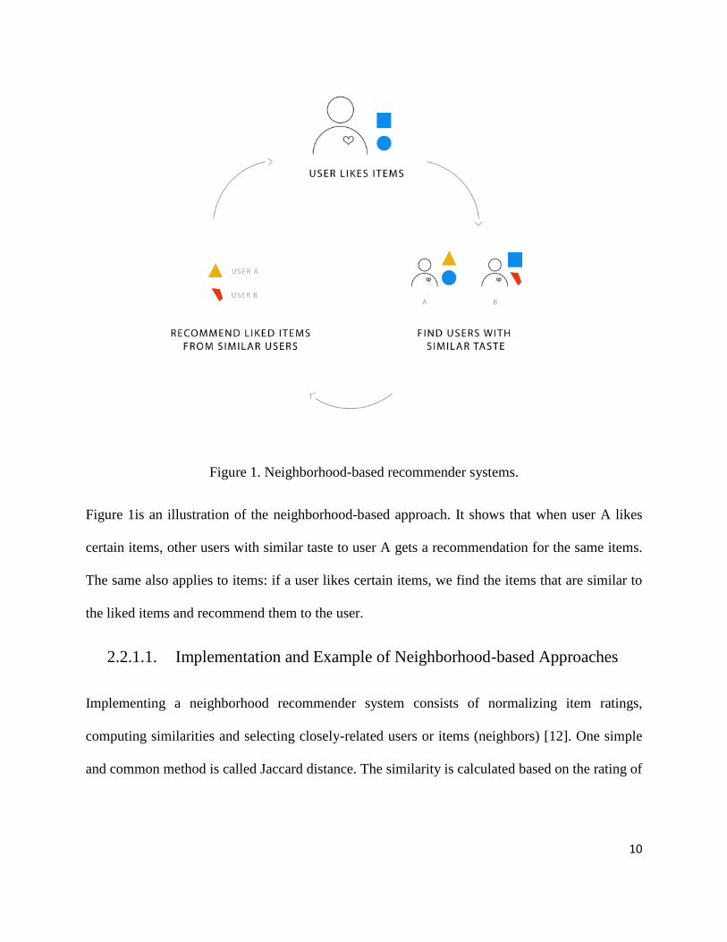
Figure 1. Neighborhood-based recommender systems.

Figure 1is an illustration of the neighborhood-based approach. It shows that when user A likes

certain items, other users with similar taste to user A gets a recommendation for the same items.

The same also applies to items: if a user likes certain items, we find the items that are similar to

the liked items and recommend them to the user.

2.2.1.1. Implementation and Example of Neighborhood-based Approaches

Implementing a neighborhood recommender system consists of normalizing item ratings,

computing similarities and selecting closely-related users or items (neighbors) [12]. One simple

and common method is called Jaccard distance. The similarity is calculated based on the rating of

11

items that users have in common. This assumes that similar users rate items in a similar manner

and vice versa.

Another method for similarity measurement is Cosine similarity. It calculates the similarity

between two users by dividing the dot product of two vectors by the product of their dimensions.

The equation for cosine similarity between two users 𝑎 and 𝑏 is below:

Eq. 2.1

cos(𝑎, 𝑏) = 𝑎 . 𝑏

||𝑎|| ||𝑏||=

∑ 𝑟𝑎𝑖 × 𝑟𝑏𝑖 𝑁𝑖=1

√∑ 𝑟𝑎𝑖2 𝑁

𝑖=1 × √∑ 𝑟𝑏𝑖2 𝑁

𝑖=1

𝑎 and 𝑏 represents the two users, 𝑟𝑎𝑖 and 𝑟𝑏𝑖 represents the rating for item 𝑖 by user 𝑎 and 𝑏

respectively. 𝑁 is the total number of items in the dataset.

Cosine similarity measures the angles between the two user vectors. For example, cos (a, b) = 1 if

vector a and vector b are the same and cos (a, b) = -1 if they are not the same.

We present some ratings in table 2.1 that are normalized by item centering normalization

technique. For each user, we subtract from the rating for each item the average rating of the user.

Normalization is done here to convert user’s ratings to a global or universal scale [12]. The zero

values in the table mean no rating available for the corresponding movies.

Movie 1 Movie 2 Movie 3 Movie 4 Movie 5

John 0 -2.333 0 1.667 0.667

Frank 0 2.333 0 -1.667 - 0.667

Eric 1.667 0.667 0 -2.333 0

12

Bill -2.333 0 0.667 0 1.667

Thomas 1 1 0 -2 0

Tosin 0 -1 0 1 0

Table 2.1. Normalized User × Item matrix showing the user’s ratings for movies.

To show how cosine similarity works, we compare John and Frank using cosine similarity,

cos (𝐽𝑜ℎ𝑛, 𝐹𝑟𝑎𝑛𝑘) = (−2.333 × 2.333) + (1.667 × −1.667) + (0.667 × −0.667)

√2.3332 + −1.6672 + −0.6672 × √−2.3332 + 1.6672 + 0.6672

= −1

The similarity between Frank and Eric is shown below:

cos(𝐹𝑟𝑎𝑛𝑘, 𝐸𝑟𝑖𝑐) = (0.667 × −2.333) + (−2.333 × −1.667)

√2.3332 + −1.6672 + −0.6672 × √1.6672 + 0.6672 + 2.3332

≈ 0.628

Looking at the rating matrix in table 2.1, Frank and Eric rated almost the same movies except for

movie 1 and movie 5, and their ratings were fairly close. But John and Frank have opposite ratings

for the same rated items; their similarity is -1. Also, when we look at the similarity between items,

we would observe the ratings of movie 2 and movie 4 and conclude that movie 2 and movie 4 are

unrelated. The problem with cosine similarity is that it doesn’t consider the differences in the mean

ratings of the users [12].

Pearson correlation coefficient similarity provides an adjustment to the cosine similarity. The

equation below shows the Pearson correlation similarity between user 𝑎 and 𝑏:

Eq. 2.2

13

PC(𝑎, 𝑏) = ∑ (𝑟𝑎𝑖 − 𝑟�̅�) × ( 𝑟𝑏𝑖 − 𝑟�̅�) 𝑁

𝑖=1

√∑ (𝑟𝑎𝑖 − 𝑟�̅�)2 𝑁𝑖=1 × √∑ (𝑟𝑏𝑖 − 𝑟�̅�)2 𝑁

𝑖=1

𝑎 and 𝑏 represents the two users, 𝑟𝑎𝑖 and 𝑟𝑏𝑖 represents the ratings for item 𝑖 by user 𝑎 and 𝑏

respectively. 𝑁 is the total number of items in the dataset, 𝑟�̅� and 𝑟�̅� represents the mean ratings of

users 𝑎 and 𝑏 respectively.

We compute the similarities for all users and select the k nearest neighbors (users with the highest

similarity) for each user. The set 𝑁(𝑎) contains the nearest neighbors of user 𝑎. We further divide

this set into a subset of neighbors that have ratings for item 𝑖 and represent it as 𝑁𝑖(𝑎). 𝑟𝑎�̂� is

calculated as the weighted average of the preference for item 𝑖 by all neighbor users of user a that

rated item 𝑖.

Eq. 2.3

𝑟𝑎�̂� = ∑ PC(𝑎, 𝑏) 𝑟𝑏𝑖 𝑏∈𝑁𝑖(𝑎)

∑ PC(𝑎, 𝑏) 𝑏∈𝑁𝑖(𝑎)

Where 𝑟𝑏𝑖 is the rating of user 𝑏 for item 𝑖. PC(𝑎, 𝑏) is the Pearson correlation similarity between

𝑎 and 𝑏.

Normalizing equation 2.3 by considering the differences in the mean ratings of neighbor users,

will produce a version normalized and scaled for different users below:

Eq. 2.4

𝑟𝑎�̂� = 𝑟𝑏𝑖 + ∑ PC(𝑎, 𝑏) (𝑟𝑏𝑖 − 𝑟�̅�) 𝑏∈𝑁𝑖(𝑎)

∑ PC(𝑎, 𝑏) 𝑏∈𝑁𝑖(𝑎)

Where 𝑟�̅� is the mean rating of user 𝑏, and all other symbols are as defined in previous equations.

14

As explained in [13], some users give higher ratings than others, and some items might be rated

higher than others because of how those items are perceived. Therefore, to account for the biases

in the mean user/item ratings, a baseline rating is added to adjust for global effects. We use

notation 𝑏𝑎𝑖 to represent the baseline rating that accounts for the user and item effects in the

unknown rating of item 𝑖 for user 𝑎 as shown below:

Eq. 2.5

𝑏𝑎𝑖 = 𝜇 + 𝑏𝑎 + 𝑏𝑖

𝜇 is the overall average rating, 𝑏𝑎 is the deviation of user a from 𝜇, and 𝑏𝑖 is the deviation of item

𝑖 from the average rating 𝜇. 𝑏𝑎 and 𝑏𝑖 are calculated by solving the least square problem in

equation 2.6.

Eq. 2.6

𝑚𝑖𝑛𝑏∗ ∑(𝑟𝑎𝑖 − 𝜇 − 𝑏𝑎 − 𝑏𝑖)2

𝑎,𝑖

+ 𝜏(∑(𝑏𝑎2

𝑎

+ ∑(𝑏𝑖2

i

)

Combining equation 2.5 and equation 2.6 will give us the next equation below:

Eq. 2.7

𝑟𝑎�̂� = 𝑏𝑎𝑖 + ∑ 𝑃𝐶𝑎𝑏 (𝑟𝑏𝑖 − 𝑏𝑏𝑖) 𝑏∈𝑁𝑖(𝑎)

∑ 𝑃𝐶𝑎𝑏 𝑏∈𝑁𝑖(𝑎)

2.2.2. Model-based Collaborative Filtering

Model-based methods create predictive models by learning and discovering features from the

dataset. The created models are used to make predictions for the user. A model-based collaborative

filtering method performs some offline analysis on the rating dataset to extract the models that

15

represent the latent factors that describe the relationship and characteristics between the users and

items. This model is loaded instead of the dataset during the recommendation process. When

contrasted with the neighborhood and content-based recommender systems, a model-based system

finds the distinctive features of users and items by taking a gander at the rating information. It

builds the user profiles and items profiles with the end goal of reusing both entities for subsequent

analyses.

As shown in figure 2, the utility matrix is the dataset representing users’ preferences. It is the

structured dataset processed to discover the hidden features or factors for each user in the system.

The process is repeated until the best features in the utility matrix are extracted to form a learned

model. The process of generating a model that fits the utility matrix is called learning.

Figure 2. A framework for model-based recommender systems.

16

Training the recommender system can take some amount of time, and the models can easily be

over-fitted to a dataset [14], this may cause inconsistency when using the model in a dataset other

than the training dataset. We can group approaches to learning and training into classification and

dimensionality reduction.

2.2.2.1. Foundations of Matrix factorization

Matrix factorization is a method under the model-based approach. In this section, we dive deep

into the details of two approaches that are the foundation of several matrix factorization

recommender systems. The two approaches are principal component analysis and singular value

decomposition. These techniques form the foundation of many matrix factorization based

recommender systems.

2.2.2.1.1. Principal Component Analysis (PCA)

So much information is extracted on a regular basis from different data systems, the internet, and

other sources that it turns out to be difficult to see the relations between entities and find what is

imperative easily. Principal component analysis extracts the key components and properties in

any dataset by finding the variance and detecting variables with the highest variance in the

dataset, allowing it to discard the pieces of data in the dataset that are not useful. The purpose of

the principal component analysis is to remove unnecessary data in the dataset, extract the hidden

relations and present the data in a simpler structure that is easy to understand.

To explain the principle behind PCA, we will start with two items, after that, we will generalize

for a large number of items as seen in real situations. First, let’s assume we have 𝑛 users that

17

have rated two items 𝑥 𝑎𝑛𝑑 𝑦 and we have the ratings of users for these two items in sets

𝑎 𝑎𝑛𝑑 𝑠𝑒𝑡 𝑏. The variance for each item is defined as:

Eq. 2.8

𝜎𝑎2 =

1

𝑛 ∑(𝑎𝑖 − 𝜇𝑎)2

𝑖

, 𝜎𝑏2 =

1

𝑛 ∑(𝑏𝑖 − 𝜇𝑏)2

𝑖

Where 𝑎𝑖 represents an individual user rating for item 𝑥 and 𝑏𝑖 represents an individual item rating

for item 𝑦, 𝑛 represents the total number of users, 𝑎 𝑎𝑛𝑑 𝑏 are the sets containing the user ratings

for item 𝑥 𝑎𝑛𝑑 𝑦 respectively. We define 𝜇𝑎 𝑎𝑛𝑑 𝜇𝑏 as the means of the two sets 𝑎 𝑎𝑛𝑑 𝑏.

Assuming the means of 𝑎 𝑎𝑛𝑑 𝑏 is zero then 𝜇𝑎 = 0 𝑎𝑛𝑑 𝜇𝑏 = 0, the variance for the items is

defined below:

Eq. 2.9

𝜎𝑎2 =

1

𝑛 ∑ 𝑎𝑖

2

𝑖

, 𝜎𝑏2 =

1

𝑛 ∑ 𝑏𝑖

2

𝑖

If the value of the variance is high for the two sets, then we know that the users do not agree with

the ratings for the two items 𝑥 𝑎𝑛𝑑 𝑦. If the values of the variance for the sets are low, this suggests

that the users that rated item 𝑥 agreed or have similar ratings for the item and that the users that

rated item 𝑦 agreed or have similar ratings for the item. Variance allows us to locate the important

part in the dataset and do away with a lot of the data for the item if it has a low variance. We can

shrink the rating dataset because they generally have a lot of similar rating data; and in the opposite,

if we have a high variance, then we know that almost all the dataset for the item are important, and

we might not be able to shrink the dataset.

18

To give an example of high and low variance, consider the ratings for five users on a scale of 1 to

5 for item 𝑥 as 𝑎 = (1, 1, 1, 5, 5) and for item 𝑦 as 𝑏 = (2 , 2, 3, 3, 3). We calculate the variance

𝜎𝑎2 = 3.84, and variance 𝜎𝑏

2 = 1.2. From the rating sample, we can clearly see that the ratings for

item 𝑥 have a high variance and the ratings of item 𝑦 have a low variance.

We define covariance which shows the degree of correlation between the two items 𝑥 and 𝑦 as:

Eq. 2.10

𝑐𝑜𝑣(𝑥, 𝑦) = 1

𝑛 ∑(𝑎𝑖 − 𝜇𝑎) (𝑏𝑖 − 𝜇𝑏)

𝑖

Also for covariance, we can determine if we have similar ratings and if the dataset contains

similar information for items 𝑥 and 𝑦, by checking if they have a close correlation between them.

Positive or negative covariance value indicates this. But if the covariance for the items 𝑥 and 𝑦 is

zero or tends towards zero, then 𝑥 and 𝑦 are unrelated and have different and independent.

To give an example of covariance, consider the ratings for five users on a scale of 1 to 5 for item

𝑥 as 𝑎 = (1, 2, 3, 4, 5) and for item 𝑦 as 𝑏 = (2 , 3, 4, 5, 5). We calculate the covariance

𝑐𝑜𝑣(𝑥, 𝑦) = 1.64. From the rating sample and the covariance of the two items, we can see that

𝑥 𝑎𝑛𝑑 𝑦 are correlated. If the covariance was zero then 𝑥 𝑎𝑛𝑑 𝑦 would be uncorrelated and

unrelated.

Our illustrations have been for two items thus far. We use it as a foundation and define a

generalization for hundreds, and more related items since most systems in the real world typically

have large items. We define a utility matrix 𝑋 with dimension 𝑚 × 𝑛 containing the ratings for

19

items 𝑥1, 𝑥2, … … , 𝑥𝑚 for 𝑛 users. Each column in 𝑋 represents ratings for each user and the rows

represent the ratings for items

Eq. 2.11

𝑥1 = [𝑎1, 𝑎2, 𝑎3, … … … . , 𝑎𝑛]

𝑥2 = [𝑏1, 𝑏2, 𝑏3, … … … . , 𝑏𝑛]

⋮

𝑥𝑚 = [… ]

Therefore,

𝑋 = [

𝑥1

⋮𝑥𝑚

]

Theorem 3 in [21] defined the variance for 𝑥𝑖 𝑎𝑛𝑑 𝑥𝑗 as:

Eq. 2.12

𝜎𝑥𝑖𝑗

2 = 1

𝑛 − 1 𝑋𝑖𝑋𝑗

𝑇

where 𝑋𝑖𝑇 is the transpose of matrix 𝑋𝑖.

Theorem 5 in [21] can be used here to define the covariance matrix of 𝑋 based on the variance and

covariance defined above as:

Eq. 2.13

𝑐𝑜𝑣(𝑋) = 1

𝑛 𝑋𝑋𝑇

20

The diagonal values in 𝑐𝑜𝑣(𝑋) matrix is the variance of the items in the dataset. This indicates

that the high values in the diagonal have high variance and are of great significance. The values

not in the diagonal are the covariance between two items. High covariance values have low

significance because they denote high redundancy between pairs of items and might not be useful

in the dataset.

The 𝑐𝑜𝑣(𝑋) matrix should be diagonal, having positive values in its diagonal and zero in off

diagonal places. To make 𝑐𝑜𝑣(𝑋) a diagonal matrix, we use the Theorem 6 in [21] which states

that “a symmetry S is diagonalized by an Orthogonal matrix of its eigenvectors”. The theorem

proves that:

Eq. 2.14

𝑆 = 𝐸𝐷𝐸𝑇

Where 𝐷 is a diagonal matrix and E is a matrix of eigenvectors of S. The principal components of

𝑆 are the eigenvectors of 𝐸 and the diagonals of 𝐷 are the eigenvalues. We can reduce the data in

𝑆 by selecting the eigenvectors of 𝐸 that corresponds to high eigenvalues in 𝐷. The high

eigenvectors are the important components of the data set.

2.2.2.1.2. Singular Value Decomposition (SVD)

Singular value decomposition decomposes a rating matrix 𝑋, into three matrices 𝑈, ∑, 𝑎𝑛𝑑 𝑉.

Where 𝑈 and 𝑉 represents the left and right singular vectors, and the diagonals of ∑ represents the

singular values. ∑ is a diagonal matrix whose diagonal contains the singular values.

21

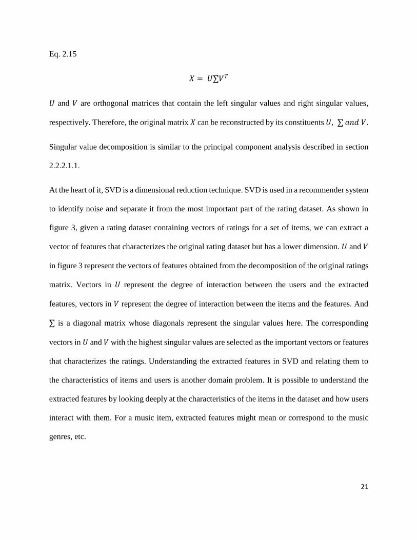
Eq. 2.15

𝑋 = 𝑈∑𝑉𝑇

𝑈 and 𝑉 are orthogonal matrices that contain the left singular values and right singular values,

respectively. Therefore, the original matrix 𝑋 can be reconstructed by its constituents 𝑈, ∑ 𝑎𝑛𝑑 𝑉.

Singular value decomposition is similar to the principal component analysis described in section

2.2.2.1.1.

At the heart of it, SVD is a dimensional reduction technique. SVD is used in a recommender system

to identify noise and separate it from the most important part of the rating dataset. As shown in

figure 3, given a rating dataset containing vectors of ratings for a set of items, we can extract a

vector of features that characterizes the original rating dataset but has a lower dimension. 𝑈 and 𝑉

in figure 3 represent the vectors of features obtained from the decomposition of the original ratings

matrix. Vectors in 𝑈 represent the degree of interaction between the users and the extracted

features, vectors in 𝑉 represent the degree of interaction between the items and the features. And

∑ is a diagonal matrix whose diagonals represent the singular values here. The corresponding

vectors in 𝑈 and 𝑉 with the highest singular values are selected as the important vectors or features

that characterizes the ratings. Understanding the extracted features in SVD and relating them to

the characteristics of items and users is another domain problem. It is possible to understand the

extracted features by looking deeply at the characteristics of the items in the dataset and how users

interact with them. For a music item, extracted features might mean or correspond to the music

genres, etc.

22

Figure 3. The singular value decomposition of X.

2.3. Context-Aware Recommender System

So far we have assumed that the predictions generated by recommender systems are legitimate and

applicable to all circumstances and situations. Many other factors could influence the preference

of a user: a user may, for example, lean towards leisurely activities at the end of the week but goes

for more business-related activities on weekdays. These factors can affect the preference of users

in a great deal. Thus, it is vital to consider the appropriate context during the process of

recommendation. It is stated in [4] that “contextual recommender system acknowledges the effect

of context in the recommendation and that the preference for an item within one context can be

different in another context. “ We use context and contextual information interchangeably

throughout this section; they mean the same.

Also, utilizing context in a recommender system gives users more confidence in predictions [16].

A recommender system might be able to explain its recommendation process regarding the

contexts used and how they utilize each one [3]. Users might tend to trust the recommender system

more because of its transparency.

23

To understand the value of context in a recommender system, we describe the typical traditional

recommender system and how context-aware recommender system extends it. Typically, a

traditional recommender system uses two-dimensional data space to estimate the rating for items

or users. The rating function R for a traditional recommender system is calculated for the (user,

item) pairs that haven't been rated by the user and defined as:

R: User x Item → Rating

Contextual recommender system extends the rating function by including one or more information

in the form of context as shown below:

R: User × Item × Context → Rating

The context used by a context-aware and driven recommender system could be fully observable,

partially-observable or unobservable contextual information. Fully observable context means that

the recommender system has full knowledge of the structures and values of the contextual

information relevant to the interaction between users and items. An example is a movie

recommender system; the contextual factors might be time or location. The structure of the time

context might be the days of the week, the month of the year, etc., and the structure of the location

might be street, city, province, state, etc.

The contextual factors relevant to the recommender system are partially observable if the system

has a partial or incomplete knowledge about them. An example is when a movie recommender

system is aware that time is a context relevant to a movie recommendation but not aware of other

relevant factors [5]. Contextual factors are unobservable in a recommender system if the system is

not explicitly aware of the contextual factors relevant to the system. A recommender system could

24

use inference and active learning techniques to extract the partially-observable and unobservable

contexts [5].

In the following sections, we discuss the context in a recommendation, ways of incorporating

contextual information into recommender systems and some important components of a context-

aware recommender system.

2.3.1. Context in Recommendation

In [3], the author described the concept of context by attempting to derive its semantics from

different fields. The consensus or common thing in all these fields or areas is how they look at

their data from a contextual standpoint, enabling them to model data and build user profiles based

on different context.

According to [4], contextual information can be in a static or dynamic form. The static form is

when the contextual information is the same over the lifetime of the recommender system.

Dynamic form is when the contextual information changes over the lifetime of a recommender

system. A function in the recommender system constantly detects the relevant contextual

information and updates as required. Dynamic form conveys a notion of adaptability, the ability

to adapt to changing contextual factors in the environment. The system detects the relevant context

and updates recommendations during the user’s interaction with the system. This may occur in

real-time where the context changes over time. Location is an example of a dynamic context that

changes as you move from one point to another.

Contexts are factors that describe the environment and situations where the activity occurs. Much

like rating data, we can acquire context data explicitly or implicitly. In the case of explicit context,

25

the user needs to specify the context deliberately. For example, a user could specify additional

information in the recommender system. This may not be dependable since it is easy for users to

overlook some relevant activities, particularly when it involves a lot of contextual information and

it is over a long period [17]. Implicit data is extracted automatically without user involvement

when a user interacts with the system. An example is the collection of information like location

coordinates, weather, user social activities, etc. Mobile phones have features like the global

positioning system (GPS) to collect location coordinates and obtain weather information from

weather services using the location obtained.

Representation of the contexts obtained follows after extracting or inferring the context. Using the

approach in [3], we show an example of a contextual data representation for a location-aware

recommender system below. We represent a context as a set of contextual dimensions, each

dimension in the set is defined by a set of attributes having a variety of granularities [3].

Given a location recommender system, we represent the set of contextual dimensions as D

containing top-level contexts. D is defined below as:

D = { Place_Category, Weather}.

We further divide each element of D to a more granular or finer level such that :

𝐷𝑝𝑙𝑎𝑐𝑒_𝑐𝑎𝑡𝑒𝑔𝑜𝑟𝑦 = {Food, Educational, Spiritual} and 𝐷𝑤𝑒𝑎𝑡ℎ𝑒𝑟 = {Winter, Summer, Fall}

Figure 4 below depicts a hierarchy tree structure showing the granularities in our example of a

location recommender system.

26

Figure 4. Hierarchy tree structure showing the granularities in a location recommender system.

2.3.2. Incorporating Contextual Information into A Recommender System

Unlike traditional recommender systems that solely rely on user preferences for some items,

context-aware recommender systems use contextual information about the activities in addition to

the user’s preferences. Incorporating context into a recommender system can be done in three

ways: contextual pre-filtering, contextual post-filtering, and contextual modeling.

27

Figure 5. Ways of incorporating contextual information in a recommender system.

Figure 5 shows a general overview of the ways contextual information is incorporated into the

recommendation process. The gray boxes represent the recommendation process in its pure form

in sequence. The rating data goes into the predictions box, which represents the engine that

performs the prediction and generates an output, the recommendations at the end of the process.

Contextual pre-filtering filters the data before it goes into the prediction engine as represented by

the orange box. Contextual post-filtering appears immediately after the prediction engine generates

its output (recommendation), refining it to generate a more useful recommendation. Contextual

modeling is incorporated directly into the prediction engine as shown by the blue box.

2.3.2.1. Contextual Pre-filtering

Contextual pre-filtering filters the rating data using the specified context before the recommender

framework computes the recommendations. Recommendations are computed by utilizing a subset

of the data that are significant to the context. This approach uses contextual information to filter

the dataset for the most relevant data (user, item, rating), before the process of recommendation

28

[3]. A good example is a user that wants to find activities in a particular season; the recommender

system only uses the preference data of the user and other users for that particular season.

In [6], a contextual pre-filtering technique based on implicit user feedback was used. This

technique incorporated micro-profiling by splitting user profiles into several smaller profiles based

on the contexts. After that, the system uses the context-based partitions for preference estimation.

Item Splitting is another pre-filtering approach. The concept is to split historical preference data

that makes up the whole dataset profile into smaller segments and make predictions based a small

segment. The major challenge of this approach is finding an efficient way to split the user profiles

into optimal and appropriate segments [6]. This item splitting technique is referred to as micro-

profiling. In [6], micro-profiling was applied on a music dataset to generate recommendations; the

datasets were collected for a two-year period; it consists of implicit user feedback data, mainly the

tracks the users of last.fm played. Multiple micro-profiles were used to model user’s profiles based

on time cycles. The smaller profiles represented the user profile for a specific time context. The

work in [6] aimed to build a recommender system that could make predictions based on the time

of the day. A comparison of the micro-profiling with the baseline prediction algorithm reveals that

the micro-profiling performed better. During the evaluation of the algorithm, user profiles were

separated into different partitions based on the time of the day; a range of time was used to group

a partition. The contextual information used had different levels of granularities. We show an

example of segmentation below. The contextual dimension used here is time, and it consists of

different contextual conditions that were used to form different contextual situations as shown in

the example.

29

An example of different pre-defined time segmentation also known as contextual situations over

contextual time factor are:

𝑇𝑇𝑖𝑚𝑒 = {𝑀𝑜𝑛𝑑𝑎𝑦, 𝑇𝑢𝑒𝑠𝑑𝑎𝑦, 𝑊𝑒𝑑𝑛𝑒𝑠𝑑𝑎𝑦, 𝑇ℎ𝑢𝑟𝑠𝑑𝑎𝑦, 𝐹𝑟𝑖𝑑𝑎𝑦, 𝑆𝑎𝑡𝑢𝑟𝑑𝑎𝑦, 𝑆𝑢𝑛𝑑𝑎𝑦}

𝑇𝑑𝑎𝑦_𝑠𝑒𝑔𝑚𝑒𝑛𝑡 = {𝑚𝑜𝑟𝑛𝑖𝑛𝑔, 𝑒𝑣𝑒𝑛𝑖𝑛𝑔} 𝑇𝑤𝑒𝑒𝑘_𝑠𝑒𝑔𝑚𝑒𝑛𝑡 = {𝑤𝑒𝑒𝑘𝑒𝑛𝑑, 𝑤𝑜𝑟𝑘𝑖𝑛𝑔 𝑑𝑎𝑦}

However, pre-filtering the rating dataset with contextual information might reduce the available

dataset for the recommendation and cause a sparsity problem in the recommendation process.

Context segments were proposed in [6] to create supersets and generalization of contextual factors

that could be used for the pre-filtering process of the rating dataset. This provides a wider dataset

that is filtered by the supersets rather than the individual contextual factors. Contextual pre-

filtering is compatible with any of the traditional 2-dimensional recommendation algorithms.

2.3.2.2. Contextual Post-filtering

The post-filtering approach applies the recommendation process on the whole dataset and after

that uses contextual information to filter the results to get the contextualized recommendations.

Post-filtering examines the preference of a user in a given context to understand the item usage

pattern for the given context and applies it to adjust the recommendation list [3]. The

recommendation list can be adjusted by either filtering out the irrelevant items for that context or

by ranking the list based on relevance in the given context.

Post-filtering allows a traditional recommendation algorithm to be used in the process of

recommendation before a filter is applied to select relevant data. For example, in a location

recommender system, if we want to recommend locations to a user based on a specific category,

30

we filter and return only the locations in the specific category or rank the recommended results

based on the category context.

Two of the most used techniques in this approach is model-based and heuristic. In model-based,

items are filtered out or re-ranked from the recommended result list by building models to predict

the probability that the recommended item is relevant to the user in a given context or set of

contexts. Filtering removes the items that have a lower probability than a set threshold from the

list and re-ranking is done based on the probability-weighted rating. Heuristic involves filtering or

re-ranking the initial recommendation results by finding common item characteristics for a given

context or set of contexts [3].

Just like the contextual pre-filtering approaches, contextual post-filtering is compatible with

traditional recommendation algorithms. This is a big advantage because any of the traditional 2-

dimensional recommendation algorithms can be used with it.

2.3.2.3. Contextual Modeling

Contextual modeling incorporates context directly into its recommendation process. Contextual

modeling uses a different approach to allow more than 2-dimensional data to be utilized to make

recommendations. The 2-dimensional data are the user and item. Contextual information can be

incorporated directly into the recommendation process alongside the user and item data. Predictive

models like context-aware matrix factorizations, regression and decision trees are examples of

contextual modeling techniques that incorporate context into their approach.

The contextual modeling approach is divided into Heuristics and model-based methods. [8]

described a contextual modeling approach called contextual neighbors that is based on

31

collaborative user filtering. Heuristic-based methods extend traditional approaches. An example is

the extension of the neighborhood approach using a multidimensional similarity method. The

heuristic-based method finds the distance between users or items with similar context. The distance

in consideration is the difference between the ratings being compared. To provide a generalized

distance measurement, the dataset is grouped into segments using the available context, and the

distance function is calculated on segments, this could help reduce sparsity where there are no

adequate data for some contexts.

Different user profiles are created based on the available contextual conditions using different

profiling methods. These contextual profiles are used to find the similarities between two users in

a given context during the process of producing contextual neighbors. This approach finds all the

nearest neighbors of a user in a given context by measuring the similarity between user’s

contextual profiles.

The work in [8] selects four different kinds of contextual neighbors. The first one has no constraint

on selection; it selects all users similar to the given user in the given context. The second method

adds a little constraint; it selects an equal number of users similar to the given user for each value

of the contextual condition based on the neighborhood size. The third method goes further by

selecting only neighborhood profiles for a given level of context; usually, the context has different

levels of granularity as explained in previous sections. The fourth method selects an equal number

of neighbors for each context level. The results of the experiment in [8] show that the first method

performs better than the rest because of the unconstrained selection.

32

Several methods have extended the traditional model-based approaches for two-dimensional to

incorporate contextual information; examples are Bayesian preference models, support vector

machines, etc.

33

3. Related Work

In this chapter, we do a review of several works on recommender systems that have incorporated

matrix factorization and contextual information into their process of recommendations. After that,

we discuss coupled matrix factorizations. Because coupled matrix factorization is an extension of

matrix factorization, we review some related works on traditional matrix factorization to set the

stage and then we proceed to discuss some related works in context-aware matrix factorization

methods. After that, we review some works on coupled matrix factorization; which serves as the

core of our proposed methods.

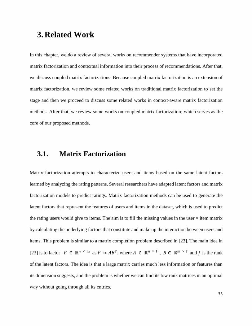
3.1. Matrix Factorization

Matrix factorization attempts to characterize users and items based on the same latent factors

learned by analyzing the rating patterns. Several researchers have adapted latent factors and matrix

factorization models to predict ratings. Matrix factorization methods can be used to generate the

latent factors that represent the features of users and items in the dataset, which is used to predict

the rating users would give to items. The aim is to fill the missing values in the user × item matrix

by calculating the underlying factors that constitute and make up the interaction between users and

items. This problem is similar to a matrix completion problem described in [23]. The main idea in

[23] is to factor 𝑃 ∈ ℝ𝑛 × m as 𝑃 ≈ 𝐴𝐵𝑇, where 𝐴 ∈ ℝ𝑛 × f , 𝐵 ∈ ℝ𝑚 × f and 𝑓 is the rank

of the latent factors. The idea is that a large matrix carries much less information or features than

its dimension suggests, and the problem is whether we can find its low rank matrices in an optimal

way without going through all its entries.

34

The use of SVD was proposed for factorization in [24], [36] and [37]. Sweeny, Lester et al. [24]

discussed in details how to estimate low factors from a dataset using SVD. The authors in [24]

used a student-course grade dataset to illustrate their method. They decomposed the dataset into a

low rank space resulting in two sets of less noisy latent vectors representing student and courses.

Predicting a grade for a student was a matter of multiplying the course feature vector with the

student feature vector.

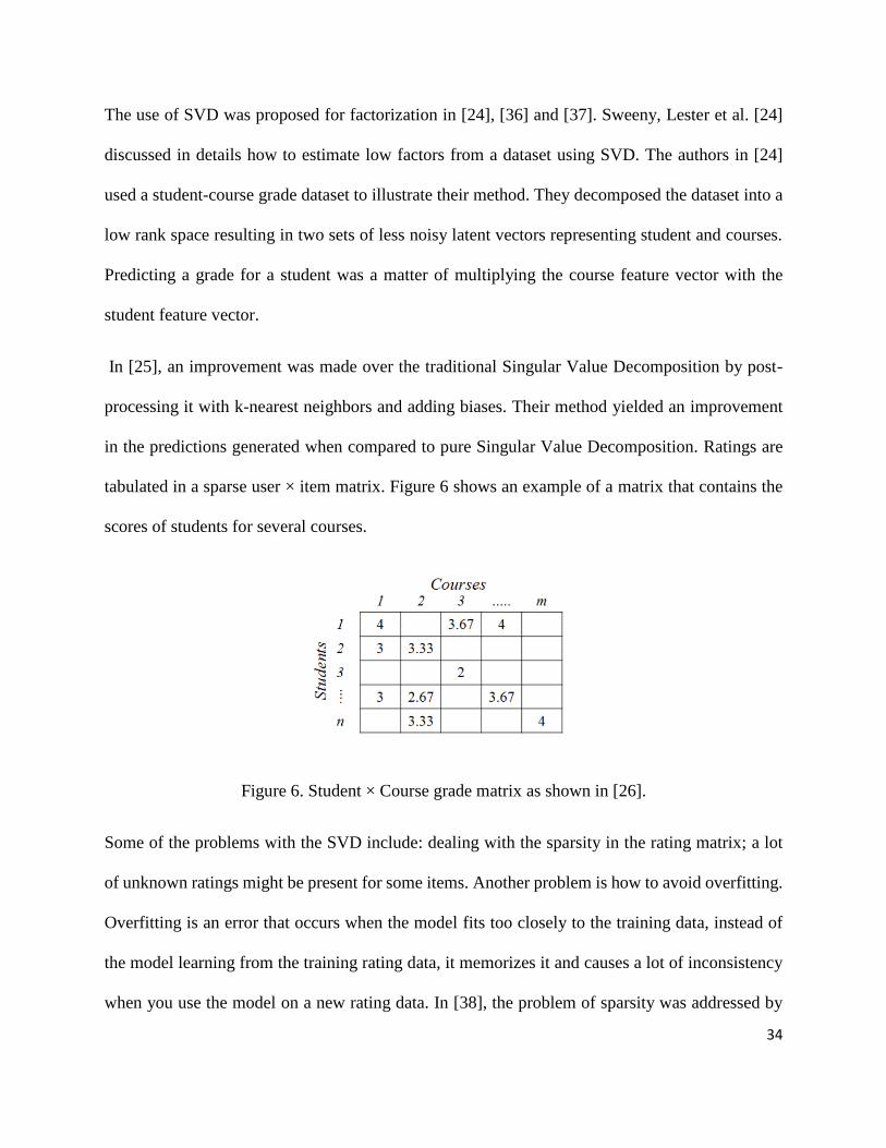
In [25], an improvement was made over the traditional Singular Value Decomposition by post-

processing it with k-nearest neighbors and adding biases. Their method yielded an improvement

in the predictions generated when compared to pure Singular Value Decomposition. Ratings are

tabulated in a sparse user × item matrix. Figure 6 shows an example of a matrix that contains the

scores of students for several courses.

Figure 6. Student × Course grade matrix as shown in [26].

Some of the problems with the SVD include: dealing with the sparsity in the rating matrix; a lot

of unknown ratings might be present for some items. Another problem is how to avoid overfitting.

Overfitting is an error that occurs when the model fits too closely to the training data, instead of

the model learning from the training rating data, it memorizes it and causes a lot of inconsistency

when you use the model on a new rating data. In [38], the problem of sparsity was addressed by

35

the imputation of the rating matrix to make the rating matrix dense, imputation, on the other hand,

might misrepresent the data. The works in [14] and [39], suggested directly modeling the observed

rating matrix and avoid overfitting by regularization. The methods involve adding a constant

parameter to control the magnitude of the user and item latent feature vectors and finding the local

minimum of the regularized squared error.

A lot of the approaches and methods stated in this section uses explicit dataset as opposed to our

method that uses implicit feedback as our dataset. Implicit data can be easily extracted from user’s

activities. It is difficult to collect explicit feedbacks because they require user surveys and several

other user-facing methods to collect feedback from users. The major addition of our approaches is

the incorporation of contexts which is additional information. By coupling the additional

information with the observed rating through joint factorization, we hope to improve the prediction

accuracy.

3.2. Context-Aware Matrix Factorization Methods

We categorize context-aware recommender systems into contextual pre-filtering, post-filtering and

modeling according to [3] as discussed in the previous chapter. The proposed model in this thesis

is under the contextual modeling classification. The proposed context-aware hierarchical Bayesian

model in [30] is an example of a contextual modeling approach. The paper proposed grouping

users and item together based on context; this is similar to how our proposed methods group items

based on context before the factorization process.

36

A context-aware recommender method considers contextual information to generate

recommendations with some contextual effects depending on how deep the context is integrated

into the method. In [27], some context-aware matrix factorization (CAMF) techniques were

developed to capture the interaction between the ratings and some contextual factors. The methods

proposed by the authors measure the relevance of the contextual factors on the ratings based on

three different assumptions. Three models were developed to capture the influence of each

contextual condition on the user ratings.

The first model in [27] is called CAMF-C; it assumes that each contextual condition has a uniform

influence over all the items. That is, the effect of each contextual condition over user ratings is the

same for all items. A single parameter represents the effect for all items in a contextual condition.

The total number of parameters is the sum of all contextual conditions of each contextual factor.

Each parameter measures the deviation from the standard rating as a result of the contextual

condition.

The second model in [27] is called CAMF-CI, it assumes that each contextual condition influences

the ratings for all items. This means that the effect of each contextual condition is different for all

items. This model introduces a large number of parameters, for each contextual condition and item

pair, a parameter is used to model the deviation of the rating. This model provides better prediction

according to the authors in [27].

The third and last model is called CAMF-CC, it groups items into categories and assumes that the

influence of each contextual condition is the same for each item category. A parameter is used to

model the deviation for each contextual factor and item category pair [27].

37

A contextual condition in [27] refers to a value of a contextual factor; we further explain what it

means later in this section. The results of the experiments in [27] show that the CAMF-CC model

performs better generally when compared to the other models in their work and another baseline

context-aware factorization model. The problem with CAMF-CI is that it is too complex, thereby

reducing prediction accuracy. One limitation of CAMF-CC when compared to our model is that it

can only be used for items grouped in categories. CAMF-CC assumes that a domain expert can

effectively group items, this becomes a problem when items cannot be efficiently grouped. In

contrary, our proposed methods group ratings based on the contextual conditions they occurred.

For example, we group ratings of music played in the morning; morning here is a contextual

condition of the time contextual factor. This doesn’t require a domain expert and makes the

grouping and splitting process transparent. Another limitation of the methods in [27] is they

capture only the influence of the contextual conditions on items. Our approach captures the

influence of contextual conditions on users and items instead.

In [28], some correlation-based context-aware matrix factorization methods were developed and

claimed to be an improvement over the models in [27], measuring correlation rather than rating

deviation. The contextual correlation based CAMF measures the correlation between two

contextual situations, the assumption is that two similar contextual situations for a user will

produce similar recommendations for that same user.

A contextual situation in [28], is a set of contextual conditions, where each element is a contextual

condition of a contextual dimension. A contextual dimension represents the contextual variables

(contexts) or factors in the system, e.g., time, location, etc. A contextual condition represents a

value of a contextual factor. For example, the contextual conditions of time could be weekday,

38

weekend, etc., depending on how it is partitioned. The correlation measured in [28] is between two

contextual situations where one is empty. The contextual correlation was later integrated into the

matrix factorization process.

Three different models were developed, namely independent context similarity (ICS), latent

context similarity (LCS) and multidimensional context similarity (MCS). ICS measures the

relationship between two contextual situations as the product of the correlations among different

dimensions. It assumes that contextual dimensions are independent and therefore only calculates

the correlation between contextual conditions in the same contextual dimension.

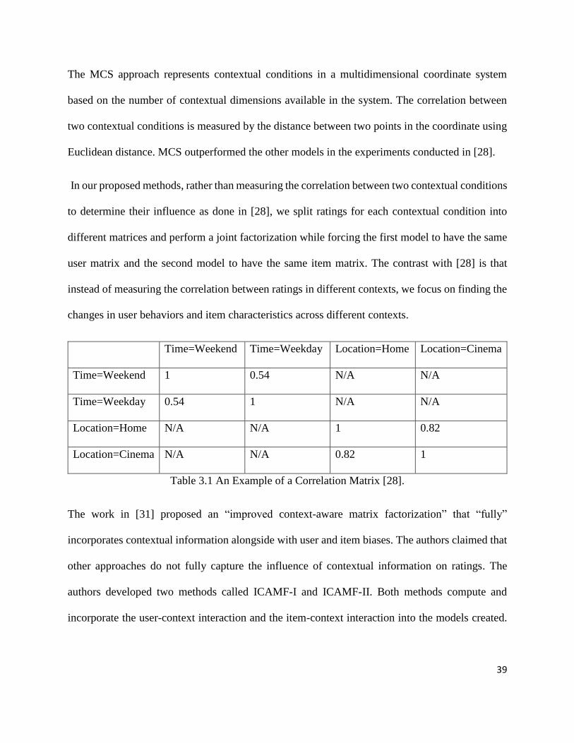
We give an example of two contextual dimensions: time and location, and two contextual

situations: {Time = “weekend”, Location = “university”} and {Time = “weekday”, Location =

“home”}. Table 3.1 shows a detailed example of correlation between contextual conditions where

the correlation between the same condition shows a perfect correlation of value 1 and “N/A” shows

that no correlation between contextual conditions belonging to different contextual dimensions.

As an example, the contextual correlation is the correlation between Time = “weekend” and Time

= “weekday” multiplied by the correlation between location = “university” and location = “home.”

The correlation values are learned in the minimization task of the factorization alongside other

values. LCS attempts to solve the problem of calculating the correlation for new contextual

conditions when they haven’t been learned in the training data. The authors chose five latent

factors, and each contextual condition is represented by a vector containing the weights of these

latent factors which are learned during the minimization process. The correlation between two

contextual situations is calculated by the dot product of the two contextual condition vectors.

39

The MCS approach represents contextual conditions in a multidimensional coordinate system

based on the number of contextual dimensions available in the system. The correlation between

two contextual conditions is measured by the distance between two points in the coordinate using

Euclidean distance. MCS outperformed the other models in the experiments conducted in [28].

In our proposed methods, rather than measuring the correlation between two contextual conditions

to determine their influence as done in [28], we split ratings for each contextual condition into

different matrices and perform a joint factorization while forcing the first model to have the same

user matrix and the second model to have the same item matrix. The contrast with [28] is that

instead of measuring the correlation between ratings in different contexts, we focus on finding the

changes in user behaviors and item characteristics across different contexts.

Time=Weekend Time=Weekday Location=Home Location=Cinema

Time=Weekend 1 0.54 N/A N/A

Time=Weekday 0.54 1 N/A N/A

Location=Home N/A N/A 1 0.82

Location=Cinema N/A N/A 0.82 1

Table 3.1 An Example of a Correlation Matrix [28].

The work in [31] proposed an “improved context-aware matrix factorization” that “fully”

incorporates contextual information alongside with user and item biases. The authors claimed that

other approaches do not fully capture the influence of contextual information on ratings. The

authors developed two methods called ICAMF-I and ICAMF-II. Both methods compute and

incorporate the user-context interaction and the item-context interaction into the models created.

40

The first one (ICAMF-I), incorporates a global rating average, an item and user bias that aren't

affected or influenced by the contextual factors.

The second method (ICAMF-II) built on the first method to incorporate item and user biases that

changes over different contextual conditions. The item and user biases are modeled as the sum of

all item and user bias over each contextual condition. Our methods measure and incorporate item

and user biases for each contextual condition rather than as a sum. As an improvement to [31], we

learn the item and user biases parameter for each contextual condition alongside the latent factors

during training; this makes our contextual item and user biases more accurate and evolving as the

rating behavior changes.

The authors in [32] created a context-aware recommender system that predicts the utility of items

in a particular context. A tuple of user, items, context, and utility was used as the data structure to

represent the problem of estimating the utility for a tuple. The utility of an item in a specified

context is a function of its latent representation which is the column vector of the feature

representation of the items and contextual factors. The Gaussian process was used to model the

utility function.

3.3. Coupled Matrix Factorization

Coupled matrix factorization is an approach that performs a joint factorization of two or more

matrices. Several attempts have been made to develop different variants of coupled matrix

factorization methods in [40], [41] and [33]. However, our methods are the first and only context-

aware coupled matrix factorization as far as we can tell. The work in [40] defines a coupled matrix

41

factorization method that serves as the foundation of our proposed work. In [40] and [41], a

coupled matrix factorization model was developed for factorizing two matrices by performing a

joint matrix factorization of two matrices at the same time and minimizing using the gradient-

based optimization method.

During the factorization of the two matrices, both matrices could share a common factor matrix.

The idea for our work came from the common factor in [40]. However, we developed two models

with two different variants of the common factor matrix in [40]. In our proposed methods, we use

the term “common user factor” in our first model. The idea is that we assume a user’s taste remains

consistent across different contextual conditions, but the item characteristics change in different

contextual conditions. The second model assumes the characteristics of items remain the same

over different contextual conditions but the user taste changes. We provide a detailed explanation

of our two proposed methods in chapter 4.

Another improvement we added to [40] is the addition of contextual user and item biases. The

method in [40] doesn’t incorporate any bias. The reason for item and user bias is because, in the

rating dataset, the rating dataset is affected by some users or items that have extremely high or low

ratings. This doesn’t model the general opinion. We incorporate bias to neutralize these effects by

accounting for the influence of those biases. Finally, we incorporate contextual information into

our models, making our work the first and only context-aware coupled matrix factorization.

“Coupling” according to [33] and [41] means the relationship among attributes of items in a

dataset. They created a coupled similarity method that measures the similarity between attributes

and characteristics of items to identify the relationship in the dataset. They incorporated the

coupled similarity method into the matrix factorization method to form a coupled item-based

42

matrix factorization. We use the term “coupling” differently in our work; we use “coupling” to

describe a process that jointly combines the factorization of different contextual matrices. We think

our definition provides a better representation of the term “coupling” which means to combine or

join. Our proposed models add user and item biases which were not added in [33] and [41]. We

do not compare our methods to the coupled matrix factorization methods discussed here because

they do not incorporate contextual information. There is no logical justification for comparison

because it would be like comparing mangoes to apples because our proposed methods generate

recommendations suitable for contextual conditions. We compare our methods to context-aware

approaches only.

43

4. The Method

Matrix factorization techniques, as seen in chapter two and three are utilized in building

recommender systems, especially in model-based approaches [18]. Researchers in the field of

recommender systems have widely adapted and explored matrix factorization to some specific

domains in recommender systems.

Time, location and weather provide useful contextual information in certain systems that can be

exploited to provide better recommendations. For example, we can assume that users who listen

to the same or very similar songs around the same time of the day say in the evening or morning,

have more similar music taste and likely to be more predictive for each other. A user might like a

song in the morning or certain days of the week but might not be so much interested in the same

song in a different period of the day or day of the week. This is an example of how time can be

used as contextual information in music recommendation.

The core idea underlying our context-aware coupled matrix factorization is, a way to incorporate

the effects of relevant contextual information into the traditional matrix factorization method for

producing better contextual based results. We focus on producing better predictions in a contextual

condition rather than globally. We have defined contextual factors and conditions already in

previous chapters, but we will give further explanations in this chapter on how we incorporate

them to produce better prediction accuracy for different contexts.

To explain the methods developed in this thesis, we formulate the problem we are trying to solve

as a contextual rating prediction problem. Given a dataset containing the ratings of users for certain

items along with contextual information, e.g., time, our goal is to develop two models that predict

44

the rating a user would give to an item in different contextual conditions and compare the

developed models with each other and other models.

We propose two context-aware coupled factorization methods in this thesis. The coupling part of

our method is founded upon the approach in [40] which we explain in detail in this chapter. In the

first section 4.1, we explain the foundation of our methods, introduce the recommendation problem

and provide an overview of the proposed methods. In section 4.2, we explain how we group the

ratings into different contextual matrices. Sections 4.1 and 4.2 also introduce some notations that

we will use throughout this chapter. In section 4.3, we provide a detailed explanation of our

proposed context-aware coupled matrix factorization with common user factors. Section 4.4

provides a detailed explanation of our proposed context-aware coupled matrix factorization with

common item factors. Section 4.5 details the addition of contextual user and item bias to our

proposed methods.

4.1. Foundations and Overview of the Proposed

Methods.

We define related symbols and notations to be used throughout this chapter in this section and

provide the foundation for our proposed methods to enable us to set the stage for this chapter,

understand the improvements made by our proposed methods and appreciate the importance of

these improvements in predicting ratings.

45

We denote the user × item matrix which contains user ratings for items and serves as the primary

source of information as 𝑅. In our case, this contains all ratings without considering the context,

making it a sample dataset containing only the ratings for users and items.

The foundation of our model is in matrix factorization, and as discussed in chapter 3, the goal of

matrix factorization is to compute the latent factors of a matrix. The goal of a pure traditional

matrix factorization is to find the factors 𝐴 and 𝐵 such that, 𝑅 ≈ 𝐴𝐵𝑇 and �̂� = 𝐴𝐵𝑇. 𝑅 is the

observed rating (sample dataset) matrix and �̂� is the matrix of the predicted ratings. �̂� ∈ ℝ𝐼 × J

where 𝐼 and 𝐽 denote the number of users and items respectively. The task is to compute the

predicted rating matrix �̂� by computing the mappings of users and items to factors 𝐴 and 𝐵.

Using a pure traditional matrix factorization without the incorporation of context or coupled

factorization, the objective function to compute the predicted rating �̂� is given as:

Eq. 4.1

�̂� = 𝐴𝐵𝑇

Where �̂� is the predicted rating matrix, 𝐴 and 𝐵 are the low factor matrices of �̂�, they represent

the interaction between users/items and the latent factors. The factors represent what characterizes

the items and the user behaviors in relation to items. 𝐴 ∈ ℝ𝐹 represents the relationship between

users and the latent factors, 𝐵 ∈ ℝ𝐹 represents the relationship between items and the latent

factors. The term “latent” here means “hidden”, the factors are discovered through this process

and they are the same factors for both users and items. Once we have these factors, we can use

them to predict the rating a user would give an item. 𝐹 is the dimension of the latent factors, 𝐵𝑇 is

the transpose of matrix 𝐵.

46

The rating �̂�𝑢𝑖 for a user 𝑢 and item 𝑖 is denoted by:

Eq. 4.2

�̂�𝑢𝑖 = 𝐴𝑢𝐵𝑖𝑇

Where �̂�𝑢𝑖 is an entry in the predicted rating matrix for user 𝑢 and item 𝑖, 𝐴𝑢 denotes the user

vector corresponding to user 𝑢, representing the interaction between the user 𝑢 and the latent

factors. 𝐵𝑖 denotes the item vector corresponding to item 𝑖, representing the degree the item

possesses the corresponding factors. The dot product �̂�𝑢𝑖 is the predicted rating.

The prediction task/problem is how to generate the latent factors and compute the mapping of users

and items to factor matrices 𝐴 and 𝐵.

With the understanding of the pure matrix factorization, our methods jointly factorize and

incorporate contextual information into the process of matrix factorization to generate latent

factors specific for contextual conditions. We show it in our proposed context-aware coupled

matrix factorization models in section 4.3 and 4.4.

Our approach derives from the work done in [40]. We use the coupled matrix factorization idea in

their work, but the model developed in [40] was not developed for making recommendations and

does not incorporate contextual information. Our proposed methods, groups the rating dataset into

its contextual conditions (the concept of contextual conditions was explained in the previous

chapter) and jointly factorizes the contextual matrices, hence the word “coupled”.

Some of the additions we made to the approach in [40] are: incorporating contextual information,

factorizing in a way to force the contextual condition matrices to have the same user factors, the

addition of regularization to avoid overfitting during training, and the addition of contextual user

47

and item biases. We add regularization to ensure that the predicted rating model can be generalized

as much as possible to be able to predict unknown ratings. Although regularization is our addition

to the model in [40], it is by no means a new approach, many works have used it in the area of

recommender systems.

4.2. Contextual Matrices and Dataset Grouping

Here we explain the method used to group a given dataset containing ratings with specified

contexts. The contextual factors must be fully observable, meaning we assume that we have full

information about the contextual factors relevant to our recommender system or ratings. A

contextual factor is a distinct context that is relevant to the user-item rating. Time is the only

contextual factor in the training dataset we used to perform our experiment. A context condition

represents a value of the contextual factor.

Given a dataset with 𝑘 contextual factors where 𝑘 ≥ 1, let 𝐶1, … . , 𝐶𝑘 represent the set of

contextual factors such that 𝐶𝑘 contains the contextual factors for the 𝑘-th contextual factor. 𝐶𝑘𝑙 is

the 𝑙-th contextual condition for the 𝑘-th contextual factor. For example, in our training dataset,

we have just one contextual factor with three contextual conditions such that 𝐶1 =

(𝑚𝑜𝑟𝑛𝑖𝑛𝑔, 𝑎𝑓𝑡𝑒𝑟𝑛𝑜𝑜𝑛, 𝑒𝑣𝑒𝑛𝑖𝑛𝑔) is the Time contextual factor and 𝐶11 = 𝑚𝑜𝑟𝑛𝑖𝑛𝑔, is a

contextual condition of Time.

We introduce the rating matrix 𝑅𝑘𝑗 to denote the matrix containing the ratings for the 𝑘-th

contextual factor and 𝑙-th contextual condition for all users and items. We call this matrix a

contextual condition matrix. For simplicity, we assume and limit our methods to incorporate only

48

one contextual factor containing three contextual conditions. The evaluation and experiments

conducted in chapter 5 are based on this assumption. Hence, 𝑅11, 𝑅12, and 𝑅13 represents the

rating matrices for each contextual condition we use throughout this chapter. We refer to these

matrices as contextual condition rating matrices. Each contextual condition rating matrix is formed

by grouping together the ratings in the whole dataset that occurred in that contextual condition to

form a subset. For example, in our training dataset, where we group together the counts of the artist

played in the morning to form a morning contextual rating matrix.

4.3. Context-Aware Coupled Matrix Factorization with

Common User Factors

In this section, we explain our proposed model called context-aware coupled matrix factorization

with common user factors. We use the term “common user factors” because we make the

contextual condition rating matrices to have the same user latent factors by compelling the user

factor matrix of each contextual condition rating matrix to be the same. We coin the name of the

method in this section to illustrate the latent user factors shared by all the contextual condition

rating matrices.

The rationale for this approach is based on the assumption that to incorporate the effect of context,

we assume that during user interaction, the effect of context on ratings reflects only on items. That

is, across different contextual conditions, the taste of users remain the same while the suitability

of items differs. An item might not be suitable in a context due to its characteristics. Since a rating

is a weighted product of the user and item latent factor matrices, the changes in ratings are largely

49

due to different values of item factors across the contextual conditions. Hence, in modeling the

user-item-context interaction, the effect of context on the rating is reflected only on items. Our

assumption makes sense in certain scenarios because some items are seasonal or suitable in certain

conditions.

In this section, we define the objective function for our context-aware coupled matrix factorization

with common user factor; this function is what computes the latent factors. The function generates

the latent factors by minimizing the prediction error as shown later in this section.

Our method extends the approach in [40] by jointly factorizing 𝑅11, 𝑅12 and 𝑅13 , and sharing

the same user factor matrix with all contextual condition matrices such that, 𝑅11 ≈ 𝐴𝐵𝑇, 𝑅12 ≈

𝐴𝐶𝑇 and 𝑅13 ≈ 𝐴𝐷𝑇. 𝐴 is the common user factor shared by the contextual condition matrices,

where 𝐵, 𝐶 and 𝐷 are the latent item factors of the observed contextual condition rating

matrices 𝑅11, 𝑅12 and 𝑅13 consecutively.

The objective of our method is to generate the latent factors and compute the mapping of users and

items to factor matrices 𝐴, 𝐵, 𝐶 and 𝐷. Once we have done that, then we can predict ratings for

users and items in a contextual condition, such that, �̂�11 = 𝐴𝐵𝑇, �̂�12 = 𝐴𝐶𝑇, and �̂�13 = 𝐴𝐷𝑇. �̂�11,

�̂�12 and �̂�13 are the predicted ratings for each contextual condition. We do this by defining and

solving a minimization problem that minimizes the prediction error to a local minimum. In the

simplest form, the difference between the observed rating and the predicted rating called the

prediction error denoted by 𝑒 is defined in [42] Eq. 2 as:

Eq. 4.3

𝑒 = 𝑅 − �̂�

50

Therefore, for each user-item-contextual condition rating pair, the prediction error in its simplest

form is defined as:

Eq. 4.4

𝑒𝑢𝑖𝑐𝑘 = 𝑅𝑢𝑖𝑐𝑘 − �̂�𝑢𝑖𝑐𝑘

Where 𝑅𝑢𝑖𝑐𝑘 represents the observed contextual conditional rating by user 𝑢 for an item 𝑖 in

contextual condition 𝑐𝑘. �̂�𝑢𝑖𝑐𝑘 is the corresponding predicted or computed rating for a contextual

condition rating by user 𝑢 for an item 𝑖 in contextual condition 𝑐𝑘.

Building on Eq. 4.4, we define our proposed context-aware coupled matrix factorization with

common user factors objective function that incorporates joint factorization as an extension of Eq.

1 of [40] as:

Eq. 4.5

𝐿 = ‖𝑅11 − (𝐴 × 𝐵𝑇)‖2 + ‖𝑅12 − (𝐴 × 𝐶𝑇)‖2 + ‖𝑅13 − (𝐴 × 𝐷𝑇)‖2

Where ‖ ‖ denotes the Frobenius norm for matrices used as a loss function, 𝐴 is the common user

factor matrix that contains the mapping of users to the latent factors, 𝐵, 𝐶 and 𝐷 are the latent item

factors of 𝑅11, 𝑅12 and 𝑅13 containing the mapping of items to latent factors. The coupling can

be seen here in the joint factorization process. The object function is solved as an optimization

problem to minimize the prediction error while computing and learning the latent factors. This

process generates our low latent factor matrices.

51

We already stated that 𝐴 represents the relationship between users and the latent factors that

determine 𝐵, 𝐶 and 𝐷 denotes the latent vectors, representing the relationship between the items

and latent factors for different contexts.

We modify our objective function in Eq. 4.5 by adding regularization to avoid overfitting during

training, so that the prediction rating model can be generalized as much as possible to be able to

predict unknown ratings. Regularization is done to penalize the magnitude of the low latent factors

computed in the objective function.

We apply the constants 𝛼 and 𝛽 as used in [14] and [39] to regularize the squared error on the set

of the observed contextual condition ratings, this is defined below as:

Eq. 4.6

𝐿 = ‖𝑅11 − ( 𝐴 × 𝐵𝑇)‖2 + ‖𝑅12 − (𝐴 × 𝐶𝑇)‖2 + ‖𝑅13 − (𝐴 × 𝐷𝑇)‖2 + ( 𝛽‖𝐴‖ 2

+ 𝛼‖𝐵‖ 2 + 𝛼 ‖𝐶‖ 2 + 𝛼 ‖𝐷‖ 2)

Where 𝛼 controls the extent of regularization for the matrices 𝐵, 𝐶 and 𝐷 and 𝛽 controls the extent

of regularization for the matrix 𝐴. 𝛼 and 𝛽 are simply the penalty parameters.

To learn the latent factors in the low factor matrices, we optimize our objective function by solving

the minimization problem below:

Formula 4.5

𝑚𝑖𝑛

𝐴, 𝐵, 𝐶, 𝐷 ‖𝑅11 − (𝐴 × 𝐵𝑇)‖2 + ‖𝑅12 − (𝐴 × 𝐶𝑇)‖2 + ‖𝑅13 − (𝐴 × 𝐷𝑇)‖2 + ( 𝛽‖𝐴‖ 2

+ 𝛼‖𝐵‖ 2 + 𝛼 ‖𝐶‖ 2 + 𝛼 ‖𝐷‖ 2)

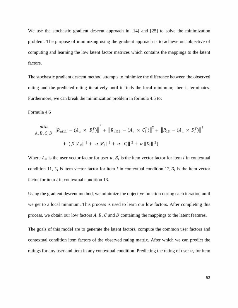
52

We use the stochastic gradient descent approach in [14] and [25] to solve the minimization

problem. The purpose of minimizing using the gradient approach is to achieve our objective of

computing and learning the low latent factor matrices which contains the mappings to the latent

factors.

The stochastic gradient descent method attempts to minimize the difference between the observed

rating and the predicted rating iteratively until it finds the local minimum; then it terminates.

Furthermore, we can break the minimization problem in formula 4.5 to:

Formula 4.6

𝑚𝑖𝑛

𝐴, 𝐵, 𝐶, 𝐷 ‖𝑅𝑢𝑖11 − (𝐴𝑢 × 𝐵𝑖

𝑇)‖2

+ ‖𝑅𝑢𝑖12 − (𝐴𝑢 × 𝐶𝑖𝑇)‖

2+ ‖𝑅13 − (𝐴𝑢 × 𝐷𝑖

𝑇)‖2

+ ( 𝛽‖𝐴𝑢‖ 2 + 𝛼‖𝐵𝑖‖ 2 + 𝛼 ‖𝐶𝑖‖ 2 + 𝛼 ‖𝐷𝑖‖ 2)

Where 𝐴𝑢 is the user vector factor for user 𝑢, 𝐵𝑖 is the item vector factor for item 𝑖 in contextual

condition 11, 𝐶𝑖 is item vector factor for item 𝑖 in contextual condition 12, 𝐷𝑖 is the item vector

factor for item 𝑖 in contextual condition 13.

Using the gradient descent method, we minimize the objective function during each iteration until

we get to a local minimum. This process is used to learn our low factors. After completing this

process, we obtain our low factors 𝐴, 𝐵, 𝐶 and 𝐷 containing the mappings to the latent features.

The goals of this model are to generate the latent factors, compute the common user factors and

contextual condition item factors of the observed rating matrix. After which we can predict the

ratings for any user and item in any contextual condition. Predicting the rating of user 𝑢, for item

53

𝑖 in a contextual condition would be a weighted sum of the common user factor vector and the

corresponding item factor vector defined as:

Eq. 4.7

�̂�𝑢𝑖𝑐𝑘 = 𝐴𝑢𝑆𝑖𝑇

Where �̂�𝑢𝑖𝑐𝑘 is the predicted rating of user 𝑢 for item 𝑖 in a contextual condition 𝑐𝑘. 𝐴𝑢 is the

common user factor vector for user 𝑢 and 𝑆𝑖𝑇 is the transpose of the associated item factor vector

for item 𝑖 in contextual condition 𝑐𝑘, 𝑆 could be 𝐵, 𝐶 or 𝐷.

For two users to have similar ratings across different contextual condition, they must have similar

common user factors and similar item ratings in a contextual condition. The core uniqueness of

this method is generating common user factors for all the contextual condition rating matrices.

All factor matrices contain the interaction/ mapping of users and items to the latent factors. Our

proposed method incorporates additional information; which in this work are contextual factors

into the factorization process, making it richer in information as compared to the traditional matrix

factorization.

4.4. Context-Aware Coupled Matrix Factorization with

Common Item Factors

In this section, we explain our proposed method called context-aware coupled matrix

factorization with common item factors. We use the term “common item factors” because it

forces the contextual condition rating matrices to have the same item latent factors by compelling

54

the item factor matrix of each contextual condition rating matrix to be the same. The name of this

method is coined in this thesis to illustrate the “item factor” shared by all contextual condition

rating matrices.

The rationale behind this approach is based on the assumption that to incorporate the effect of

context; we assume that during user interaction, the effect of context on ratings is only reflected

on users, the items maintain the same characteristics across different contextual conditions. This

means, across different contextual conditions, the taste of users changes while the characteristics

of item remain the same. And since a rating is a weighted product of the user and item latent factor

matrices, the changes in ratings is largely due to different values of user factors across the

contextual conditions. Hence, in modeling the user-item-context interaction, the effect of context

on the rating is reflected only on users. This would make sense because some items are not seasonal

or do not change characteristics in different context or conditions but a user’s taste might be

seasonal or vary in certain situations.

In this section, we show the changes in notation from section 4.3; please refer to section 4.3 for

the full description of the method. We define the objective function of our context-aware coupled

matrix factorization with common item factor by building on the work in section 4.3. In our

proposed context-aware coupled matrix factorization with common item factor, we adjust the work

done in section 4.3 by jointly factorizing 𝑅11, 𝑅12 and 𝑅13 , while forcing the matrices to share

the same item factor matrix such that, 𝑅11 ≈ 𝐵𝐴𝑇 , 𝑅12 ≈ 𝐶𝐴𝑇 and 𝑅13 ≈ 𝐷𝐴𝑇. 𝐴 is the

common item factor shared by the contextual condition matrices, where 𝐵, 𝐶 and 𝐷 are the latent

user factors of the observed contextual condition rating matrices 𝑅11, 𝑅12 and 𝑅13 consecutively.

We modify Eq. 4.4 to reflect the changes and define the objective function for this method as:

55

Eq. 4.8

𝐿 = ‖𝑅11 − (𝐵 × 𝐴𝑇)‖2 + ‖𝑅12 − (𝐶 × 𝐴𝑇)‖2 + ‖𝑅13 − (𝐷 × 𝐴𝑇)‖2 + ( 𝛽‖𝐴‖ 2

+ 𝛼‖𝐵‖ 2 + 𝛼 ‖𝐶‖ 2 + 𝛼 ‖𝐷‖ 2)

Ultimately, we define our minimization task as:

Formula 4.9

𝑚𝑖𝑛

𝐴, 𝐵, 𝐶, 𝐷 ‖𝑅𝑢𝑖11 − (𝐵𝑢 × 𝐴𝑖

𝑇)‖2

+ ‖𝑅𝑢𝑖12 − (𝐶𝑢 × 𝐴𝑖𝑇)‖

2+ ‖𝑅13 − (𝐷𝑢 × 𝐴𝑖

𝑇)‖2

+ ( 𝛽‖𝐴𝑖‖ 2 + 𝛼‖𝐵𝑢‖ 2 + 𝛼 ‖𝐶𝑢‖ 2 + 𝛼 ‖𝐷𝑢‖ 2)

Where 𝐴𝑖 is the common item vector factor for item 𝑖, 𝐵𝑢 is the user vector factor for user 𝑢 in

contextual condition 11 , 𝐶𝑢 is the user vector factor for user 𝑢 in contextual condition 12, 𝐷𝑢 is

the user vector factor for user 𝑢 in contextual condition 13.

Predicting the rating of user 𝑢 for item 𝑖 in a contextual condition would be a weighted sum of the

common item factor vector and the corresponding user factor vector defined as:

Eq. 4.10

�̂�𝑢𝑖𝑐𝑘 = 𝑆𝑢𝐴𝑖𝑇

Where �̂�𝑢𝑖𝑐𝑘 is the predicted rating for user 𝑢, for item 𝑖 in a contextual condition 𝑐𝑘. 𝐴𝑖 is the

common item factor vector for item 𝑖 and 𝑆𝑢 is the associated user factor vector for user 𝑢 in

contextual condition 𝑐𝑘, 𝑆 could be 𝐵, 𝐶 or 𝐷.

For two users to have similar ratings for a contextual condition, they must share similar user factor

values for each contextual condition. They must also share similar item ratings within the context.

56

The core uniqueness of this method is generating common item factors for all the contextual

condition rating matrices.

All factor matrices contain the interaction/ mapping of users and items to the latent factors. Our

proposed method incorporates additional information; in this work, they are contextual conditions

into the factorization process, making it richer in information as compared to the traditional matrix

factorization.

4.5. Incorporating User and Item Biases in The

Proposed Methods

To have a better and more accurate prediction of ratings, we incorporate user and item contextual

condition bias into the objective functions of both our proposed methods.

Biases are the variations in ratings due to individual effects certain users or items have. In a

recommender system, there is a tendency for certain users to give higher ratings than others and

for some items to receive higher ratings than others. This could be because some items or products

are widely perceived as better due to factors like marketing, advertisement, etc. User bias and item

bias captures the individual tendencies and variations. The item bias explains the tendency for an

item to be rated lower or higher compared to the average rating and user bias explains the tendency

for a user to rate higher or lower than the average rating.

The rating equations of our proposed methods; equations 4.7 and 4.10 calculates the ratings for an

item in a contextual condition by an interaction between user factors and item factors for the most

57

part. This doesn’t fully represent how a user rates. By incorporating item and user biases into the

equation, we can then capture the part of the rating behavior that are specific characteristics of the

individual user and item. For example, if the average rating is 3, and a user tends to rate an item 1

point higher than the average rating, and an item receives 0.5 rating less than the average rating.

The rating of the user would be the addition of the average rating, user bias and item bias which

would be 3.5 (3 + 1 + (-0.5)).

User and item bias idea is gotten from the works in [14], [19] and [20]. The baseline estimate for

an unknown rating that factors in item and user bias is defined in Eq. 1 of [14] as:

Eq. 4.11

𝑏𝑢𝑖 = µ + 𝑏𝑖 + 𝑏𝑢

Where 𝑏𝑢𝑖 is the baseline estimate for an unknown rating of item 𝑖 by user 𝑢, µ is the mean, 𝑏𝑖 is

the deviation of item 𝑖 from the mean and 𝑏𝑢 is the deviation of user 𝑢 from the mean. We propose

item and user contextual factor bias to factor in the individual effects of users and items on the

contextual condition rating calculation. We incorporate contextual condition item and user bias

into the rating equations of 4.7 and 4.10 to produce:

Eq. 4.12

�̂�𝑢𝑖𝑐𝑘 = 𝐴𝑢𝑆𝑖𝑇 + µ𝑐𝑘 + 𝑏𝑖𝑐𝑘 + 𝑏𝑢𝑐𝑘

Eq. 4.13

�̂�𝑢𝑖𝑐𝑘 = 𝑆𝑢𝐴𝑖𝑇 + µ𝑐𝑘 + 𝑏𝑖𝑐𝑘 + 𝑏𝑢𝑐𝑘

58

Where µ𝑐𝑘 represents the mean rating in the contextual condition 𝑐𝑘, 𝑏𝑖𝑐𝑘 represents the bias of

item 𝑖 in the contextual condition 𝑐𝑘, 𝑏𝑢𝑐𝑘 represents the bias of user 𝑢 in the contextual condition

𝑐𝑘

The contextual condition biases for item 𝑖 and user 𝑢 for the three contextual conditions we have

in our model are: 𝑏𝑢11, 𝑏𝑖11, 𝑏𝑢12, 𝑏𝑖12, 𝑏𝑢13, 𝑏𝑖13. Hence, we extend both objective functions and

learn the biases in the minimization task and also regularized the biases to avoid over fitting, the

extended functions of formulae 4.6 and 4.9 are:

Formula 4.14:

𝑚𝑖𝑛

𝐴, 𝐵, 𝐶, 𝐷, 𝑏𝑢11, 𝑏𝑖11, 𝑏𝑢12, 𝑏𝑖12, 𝑏𝑢13, 𝑏𝑖13 ‖𝑅𝑢𝑖11 − (𝐴𝑢 × 𝐵𝑖

𝑇) − µ11 − 𝑏𝑖11 − 𝑏𝑢11‖2

+ ‖𝑅𝑢𝑖12 − (𝐴𝑢 × 𝐶𝑖𝑇) − µ12 − 𝑏𝑖12 − 𝑏𝑢12‖

2

+ ‖𝑅13 − (𝐴𝑢 × 𝐷𝑖𝑇) − µ13 − 𝑏𝑖13 − 𝑏𝑢13‖

2+ ( 𝛽‖𝐴𝑢‖ 2 + 𝛼‖𝐵𝑖‖ 2

+ 𝛼 ‖𝐶𝑖‖ 2 + 𝛼 ‖𝐷𝑖‖ 2 + 𝛼 ‖𝑏𝑖11‖ 2 + 𝛼 ‖𝑏𝑢11‖ 2 + 𝛼 ‖𝑏𝑖12‖ 2 + 𝛼 ‖𝑏𝑢12‖ 2

+ 𝛼 ‖𝑏𝑖13‖ 2 + 𝛼 ‖𝑏𝑢13‖ 2)

Formula 4.15

𝑚𝑖𝑛

𝐴, 𝐵, 𝐶, 𝐷, 𝑏𝑢11, 𝑏𝑖11, 𝑏𝑢12, 𝑏𝑖12, 𝑏𝑢13, 𝑏𝑖13 ‖𝑅𝑢𝑖11 − (𝐵𝑢 × 𝐴𝑖

𝑇) − µ11 − 𝑏𝑖11 − 𝑏𝑢11‖2

+ ‖𝑅𝑢𝑖12 − (𝐶𝑢 × 𝐴𝑖𝑇) − µ12 − 𝑏𝑖12 − 𝑏𝑢12‖

2

+ ‖𝑅13 − (𝐷𝑢 × 𝐴𝑖𝑇) − µ13 − 𝑏𝑖13 − 𝑏𝑢13‖

2+ ( 𝛽‖𝐴𝑖‖ 2 + 𝛼‖𝐵𝑢‖ 2

+ 𝛼 ‖𝐶𝑢‖ 2 + 𝛼 ‖𝐷𝑢‖ 2 + 𝛼 ‖𝑏𝑖11‖ 2 + 𝛼 ‖𝑏𝑢11‖ 2 + 𝛼 ‖𝑏𝑖12‖ 2

+ 𝛼 ‖𝑏𝑢12‖ 2 + 𝛼 ‖𝑏𝑖13‖ 2 + 𝛼 ‖𝑏𝑢13‖ 2

59

5. Evaluation

We test our recommendation methods by performing an offline experiment. Offline experiments

are experiments conducted using datasets or data sources collected from user interaction with a

system, but the experiment process doesn’t interact with the users. Online experiments carry out

user studies and experiments that interacts with users during the process. We use implicit data; this

means data collected about the activities of users which doesn’t explicitly show intent. We explain

the characteristics of the last.fm music dataset used and after that discuss the evaluation criteria

and methods used. Finally, we discuss the results, analysis and performance of our methods and

chosen baseline methods in the test performed.

5.1. Dataset

In our experiment, we use the dataset obtained from the last.fm music website. The dataset contains

the music listening history of users. For each user, the dataset contains the tracks played by the

user and the timestamp the user listened to each track. Each track is represented by the track id,

the title of the track, the artist id, and name. The dataset contains 992 users, 176,948 artists and a

total of 19,121,228 listening entries. The last.fm dataset is an example of an implicit dataset. An

implicit dataset contains users’ activities and actions that could be used to infer users’ preference

in a system. The music listening history is an example of an implicit dataset that could be used to

infer the tracks that users like.

60

This dataset consists of tracks played by users. The average play count for a track is about two to

three per user. For simplicity, and in other to have a less sparse dataset, we assume that tracks from

the same artist are similar. Therefore, we accumulate user’s play counts per artist and predict artists

instead of tracks for users.

Studying this dataset, we found out that some users tend to listen to same artists, within the same

time periods of the day. For example, some users listen to an artist between the period of 5 pm to

11 pm. In our work, we use this dataset to study the periodical play count pattern of users.

The contextual factor in this dataset is time. We split time into three contextual conditions:

morning, afternoon and evening/night. Morning represents the period between 12 am and 11:59

am, afternoon represents the period between 12 pm and 5:59 pm while evening/night represents

the period between 6 pm and 11:59 pm. We group the dataset into three subsets, each representing

the three contextual conditions. Each subset contains the listening history within the corresponding

period.

We split this dataset into two, a training dataset and a test dataset. We use the training dataset to

train our proposed methods. We use a training and testing partition because we run the experiments

for 10, 20 and 30 latent features each through 10,000 iterations to minimize the error, this would

take a large amount of computation time for each evaluation considering the limited amount of

computing resources we have available to use. In the test dataset, we predict the artists a given

user would like in a given period. We select artists from a set of new artists not in the user’s play

history. We use the listening history data to get the play counts for an artist, in a given period. A

user with a high play count for an artist in a given period, suggests that the user likes listening to

that artist during that period.

61

5.2. Evaluation Method

To evaluate the performance of our proposed methods, we measure the prediction accuracy of our

methods on our test dataset. We randomly select 100 users for testing. We divide our test dataset

into three parts as explained in the dataset section, each containing user’s listening history for each

time contextual condition, e.g., morning, evening, etc.

The data in the test dataset is excluded from the training dataset. For each user in the training

dataset, the artist play count by the user is set to zero for the corresponding artist in the test dataset.

We do this so that we can test the prediction accuracy of our methods on artists new to the user.

In this experiment, due to the limitations of implicit dataset not explicitly showing intent [46], we

observe the user listening behavior in the dataset and came out with an assumption. Our assumption

is stated below:

1. We assume that if a user has 𝑡 play count for an artist, then the user probably likes the

artist. Parameter 𝑡 is set to the average play count for a user. This is because people tend to

play the tracks they like more. We use this assumption to infer intent from the dataset.

Because we used an implicit dataset that doesn’t explicitly state intent, we needed a way

to infer intent from the dataset.

We evaluate the prediction accuracy of our methods on the test dataset using the Mean Absolute

Error (MAE) and the Root Mean Square Error (RMSE). MAE is a popular statistical accuracy

metric used in a recommender system to measure the deviation of a prediction or recommendation

from the actual value [41]. MAE, as defined in Eq. 4 in [43], is defined below:

Eq. 5.1

62

𝑀𝐴𝐸 = ∑ |𝑃𝑢,𝑖 − 𝑟𝑢,𝑖 | 𝑢,𝑖

𝑁

𝑃𝑢,𝑖 is the predicted rating generated by our methods for user 𝑢 and item 𝑖, 𝑟𝑢,𝑖 is the actual rating

(observed rating) for user 𝑢 and item 𝑖 in the test dataset. 𝑁 is the total number of ratings in the

test dataset.

RMSE is a popular metric for evaluating the accuracy of predicted ratings by measuring the

deviation of a predicted rating from the actual value [47]. RMSE, compared to MAE penalizes

large errors and prefers smaller errors. RMSE ,as defined in Eq. 4 in [43], is defined below:

Eq. 5.2

𝑅𝑀𝑆𝐸 = √1

𝑁∑

𝑢,𝑖

(𝑃𝑢,𝑖 − 𝑟𝑢,𝑖 )2

𝑃𝑢,𝑖 is the predicted rating generated by our methods for user 𝑢 and item 𝑖, 𝑟𝑢,𝑖 is the actual rating

(observed rating) for user 𝑢 and item 𝑖 in the test dataset. 𝑁 is the total number of ratings in the

test dataset.

We compare our methods with some baseline methods that incorporate context into their

recommendation process.

The baseline methods we compare with our methods are:

a. Independent context similarity (ICS) and latent content similarity (LCS) methods of the

correlation-based context-aware matrix factorization (correlation-based CAMF) in [28].

We evaluate both ICS and LCS methods with the same training and test dataset used for

our methods. The main rationale for choosing ICS and LCS is because they are both state-

63

of-the-art context-aware matrix factorization methods, and they performed better than

some existing context-aware matrix factorization methods according to the results of the

experiment in [28]. Also, we needed methods that could generate recommendations for

different contextual conditions instead of making general recommendations. A lot of the

existing context-aware methods use context to make general recommendations. Another

reason why we choose to compare our proposed methods with ICS and LCS is to

demonstrate and confirm that incorporating changes in user behavior and item

characteristics across contextual conditions as used in our proposed methods is more

effective than generating recommendations based on the correlation between two

contextual conditions used in ICS and LCS. We discussed both ICS and LCS extensively

in section 3.2.

b. The context-aware matrix factorization (CAMF) methods in [27]. We compare our

methods with CAMF-C and CAMF-CI in [27]. These methods are both state-of-the-art

context-aware matrix factorization methods that can make recommendations for contextual

conditions. We compare our proposed methods with CAMF-C and CAMF-CI to

demonstrate and verify that our methods provide a better way to capture the influence of

context on items. We discussed both methods extensively in section 3.2.

In general, we choose the methods above because they are context-aware methods that can be used

to predict user ratings for a contextual condition.

5.3. Result and Analysis

We train our models using the training dataset to generate different latent factors with different

dimensions (number of factors). After that, we conduct a series of experiments to evaluate the

64

ability of our proposed methods to predict items for users in different contextual situations. We

run different experiments to show the performance of our methods in comparison with the chosen

baseline methods, using a different number of factors for each experiment. We provide below

analysis of the results of the experiments conducted.

In running our experiments, we observed that, while the number of iteration is directly proportional

to the effectiveness of our models, giving it a better MAE and RMSE scores, the number of

iterations is also directly proportional to the time it takes to learn and generate our latent factors.

The running time complexity of our methods is linear as a function of the number of iterations

without taking the size of the dataset into consideration. Therefore, we use 10,000 iterations which

take about 40 minutes to run for each iteration on a 4 GB RAM machine.

In choosing our parameters 𝛼 and 𝛽, we did some try-and-error to arrive at the best values because

calculating the appropriate values for these parameters has been proved to be a difficult research

problem [44]. In our experiment, we measure the sensitivity of our model to each try-and-error

value we set by measuring the MAE and RMSE at each step of the training. We observed that our

models performed better with small values of both parameters. We settled for 𝛼 = 0.6 and 𝛽 =

0.4.

We run some experiments to measure the prediction accuracy of our proposed methods and

compare them to the prediction accuracy of our chosen baseline methods using MAE and RMSE.

We set the number of latent factors to different values for each experiment to test whether the

number of latent factors extracted affects the prediction accuracy of the proposed methods and to

compare the performance of the baseline methods to our proposed methods when different

dimensions are extracted. We use 10, 20 and 30 as the dimensions of the latent factors and run

65

different experiments for each dimension. We settled for these values after running different trials

and observing that these dimensions provided the best prediction accuracies. The results are shown

in table 5.1. In the table, we observed that setting the number of factors to 30 produced the best

prediction accuracy.

We observe from our experiments that, context-aware coupled matrix factorization with common

item factors shows better prediction accuracy for all dimensions, with an average improvement of

3.75% regarding MAE and 2.15% regarding RMSE across different dimensions. Context-aware

coupled matrix factorization with common user factors show an average improvement of 2.75%

regarding MAE and 1.43% regarding RMSE across the three dimensions used. Context-aware

coupled matrix factorization with common item factors show an average performance of 25% and

20% regarding MAE and RMSE over context-aware coupled matrix factorization with common

user factors. Therefore, we conclude that our proposed methods provide good prediction accuracy,

but context-aware coupled matrix factorization with common item factors performs better.

The characteristics of the music dataset used could be an explanation for why the coupled matrix

factorization with common item factors performed better in our experiment. In a music

recommender system, most tracks would normally have the same characteristics and suitability

across different contextual situations. It is the changes in user’s taste in different conditions that

account for what users consume in certain contexts. In certain scenarios where the changes in the

consumption of items are largely due to the suitability of items across different situations, context-

aware coupled matrix factorization with common user factor might perform better.

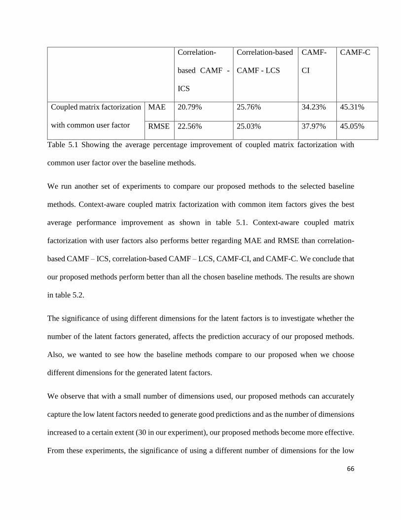
66

Correlation-

based CAMF -

ICS

Correlation-based

CAMF - LCS

CAMF-

CI

CAMF-C

Coupled matrix factorization

with common user factor

MAE 20.79% 25.76% 34.23% 45.31%

RMSE 22.56% 25.03% 37.97% 45.05%

Table 5.1 Showing the average percentage improvement of coupled matrix factorization with

common user factor over the baseline methods.

We run another set of experiments to compare our proposed methods to the selected baseline

methods. Context-aware coupled matrix factorization with common item factors gives the best

average performance improvement as shown in table 5.1. Context-aware coupled matrix

factorization with user factors also performs better regarding MAE and RMSE than correlation-

based CAMF – ICS, correlation-based CAMF – LCS, CAMF-CI, and CAMF-C. We conclude that

our proposed methods perform better than all the chosen baseline methods. The results are shown

in table 5.2.

The significance of using different dimensions for the latent factors is to investigate whether the

number of the latent factors generated, affects the prediction accuracy of our proposed methods.

Also, we wanted to see how the baseline methods compare to our proposed when we choose

different dimensions for the generated latent factors.

We observe that with a small number of dimensions used, our proposed methods can accurately

capture the low latent factors needed to generate good predictions and as the number of dimensions

increased to a certain extent (30 in our experiment), our proposed methods become more effective.

From these experiments, the significance of using a different number of dimensions for the low

67

factor matrices is to find the range of the dimensions that can effectively capture the latent factors

that best describes the behaviors of users.

Method No of latent factors MAE RMSE

Context-aware coupled matrix

factorization with common user factors

10 0.545 0.772

20 0.538 0.766

30 0.530 0.761

Context-aware coupled matrix

factorization with common item factors

10 0.479 0.698

20 0.472 0.691

30 0.461 0.683

Correlation-based CAMF - ICS

10 0.601 0.899

20 0.591 0.890

30 0.582 0.882

Correlation-based CAMF - LCS

10 0.644 0.927

20 0.638 0.922

30 0.621 0.911

CAMF-CI

10 0.752 1.152

20 0.742 1.142

30 0.701 1.101

CAMF-C

10 0.883 1.283

20 0.852 1.252

30 0.843 1.243

Table 5.2 Showing the MAE and RMSE results of the experiment conducted.

68

6. Discussion

Our work presents some improvements over traditional recommendation approaches, by

incorporating additional information called context into the process of recommendation and

making context critical rather than just some additional information. Because we make context

front and center, our proposed methods can provide recommendations that are suited towards

user’s current state or contextual condition. Some examples are recommending music tracks for

users in the morning, recommending activities suited towards a sunny day, etc.

E-commerce and content providers are seeing rapid changes in users’ taste due to lots of

information and items available on the web. If consumption of these items and information occurs

in different contexts, a context-aware recommender system can be developed based on our

proposed methods to help providers understand the changes in the taste of their users in different

contexts and provide recommendations that are useful and tailored to fit the conditions and

intentions of their users. Once we identify the contextual factors affecting the behavior of users in

an application, we can use our approach and methods to split the dataset extracted from the

application into different contextual matrices and predict what a user would like or buy in a

contextual situation. For instance, in an event recommender system, user’s location, weather

condition, time of the event, etc., are some examples of contextual factors that affect users’ choice

of an event. We can use our proposed methods to split the events users have attended in the past

into contextual factor groups and recommend events to users based on the combination of location,

weather condition and the time of the event.

69

Our proposed methods provide an important value in the era of the internet of things where we

want to make useful applications from the data generated by sensors. For instance, refrigerators,

thermostats, mobile phones, clothes, etc. when connected to the internet can send additional data

about their location and period of usage to a remote server on the internet. Our proposed methods

can leverage this contextual information to develop a recommender system that predicts and

generates contextual recommendations to the users of the connected objects. For example, a

recommender system based on our proposed methods can be developed to use the data received

from a smart refrigerator connected to the internet to recommend different food items to the user

at the different time of the day.

Our proposed models would be beneficial to recommender systems because they can provide

recommendations for new users by looking beyond the unavailable historical data and focusing on

providing recommendations based on the current circumstances and contextual condition of the

user. This can be achieved by looking at what existing users in the contextual condition have in

common and recommending that to the new user. This could help to reduce the effect of the cold

start problem, where the recommender system cannot provide recommendations for new users

because it lacks historical data about the new user.

Our proposed methods can recommend other services, products and work with different datasets

other than the music recommender system dataset used in chapter 5. Some other examples of

product categories our approach can generate recommendations for are TV shows, movies, events,

locations, etc. The same way we applied our methods to the music domain, we can apply our

methods to other domains. The contextual factors that affect the problem domain or product must

be stated and identified before applying our proposed methods to develop a context-aware

70

recommender system. One way to determine the contextual factors that affect a product is to look

at users’ behavior and purchase history. Once we can identify the contextual factors, we can apply

the method in section 4.2 to group the dataset into contextual condition matrices. The contextual

condition matrices serve as the input to both of our proposed methods.

Our methods personalize recommendations to users’ contextual situations by considering the

historical data in the specified contextual situation we wish to generate the recommendation. Our

approach to generating recommendations is based on the position in [6] that, “people have more

in common with other people in the same situation, or with the same goals than they do with past

versions of themselves.” By focusing on the preference and behavior of users in a contextual

condition, our proposed methods can predict what a user would like in a contextual condition based

on what other users in that contextual condition liked in the past.

One significant limitation of our proposed methods is scalability. Computing recommendation for

users in a big dataset requires a lot of memory and computation resources. In a domain with

hundreds of contextual factors affecting users’ behavior, computing recommendations with our

proposed methods might be a challenge. With hundreds of contextual factors, splitting the dataset

into contextual situation matrices would be a cumbersome task. Coupled matrix factorization of

hundreds of contextual matrices would require a lot of computing and memory resources. A

possible solution to this challenge is applying parallel and distributed principles to design

algorithms that would compute different pieces of our proposed methods on multiple computers

and processors. Another possible solution is precomputing and generating the models that predict

recommendation for a snapshot of the dataset and performing an incremental computation to re-

build the latest models as the dataset changes.

71

7. Conclusion and Future Work

7.1. Conclusion

In this age of big data and information explosion, providing recommendations help users to get

relevant data in an online system. Mostly found in many online systems, a recommender system

takes historical information about user’s interaction and applies an algorithm to predict what the

user would like. A context-aware recommender system is a type of recommender system that takes

into consideration information regarding the circumstance or settings around the interaction of a

user with an item when predicting what the user would like.

We aimed to develop a context-aware approach to making recommendations that are context

centric; i.e., an approach that provides recommendations based on contextual rating, the rating

given in a particular context. Therefore, our focus was to develop methods that provide

recommendations for different contexts and not general recommendations.

After evaluating our methods on the last.fm dataset, our experimental results showed that both the

proposed context-aware coupled matrix factorization methods showed a good performance on

predicting new artists for users, but the method with the common item factor showed better

prediction results. Therefore, the taste of users changes across different contexts, but the

characteristics of items don’t change that much when compared to user’s behaviors, based on our

experiments. This would make sense for certain items like music or artist; whether a user likes a

song in the morning or evening is relative to the user for the most part. This means for two users

72

to share similar artist taste in a context, they must have similar ratings or taste for the artist in the

context being considered. Our results also show that other factors like parameters of the methods

and number of iterations the method runs during the training affect the accuracy of prediction.

We compared our methods with some state-of-the-art context-aware recommendation methods,

and our proposed methods showed a fairly significant improvement over all the methods

considered. We have to mention that our method is more suited towards making predictions for

specific contexts, and might be less effective in applying contextual information to make general

predictions. Also splitting ratings into contextual groups before performing predictions make our

method more effective towards performing context centric recommendations. We also made some

assumptions during the experiment as stated in the evaluation section of the previous chapter.

These might have added some advantages to our proposed methods.

From the results of our experiments, we can deduce that jointly factorizing matrices work for

contextual rating matrices (rating matrices containing ratings for a contextual condition). Jointly

factorizing the ratings for different context also saves time, because the factorization is done at

once together. Furthermore, forcing the contextual condition matrices to have a common low factor

matrix, especially a common item low factor matrix, helps to attach the information that is not

context specific to different contextual conditions; thus, avoiding overfitting to a particular

contextual condition. This was shown in the disparity of the results obtained by the two methods

(table 5.1), and it is clear that having a common factor works but knowing which factor to share

was not evident until after performing the experiment.

One limitation of our proposed methods is, they only incorporate one context. This would be a

challenge in a domain or dataset with multiple contexts. Some scenarios would require the

73

recommender systems to incorporate multiple contexts in its recommendation process. An

example is an event recommender system with multiple contextual factors like time of the event,

location of the user and event, weather conditions, etc.

Another limitation of our proposed methods is the assumptions made by each method. The context-

aware coupled matrix factorization with common user factors model assumes users’ taste remains

the same across different contextual conditions and the context-aware coupled matrix factorization

with common item factors model assumes the characteristics of items remains the same across

different contextual conditions. There might be scenarios where users’ taste and item

characteristics change across different context. Our methods might fall short in such scenarios. An

example is a news application, users’ consumption and the characteristics of news items change

across different categories and locations. This behavior is similar for most content-based

applications.

7.2. Future Work

Our proposed methods were formulated and experimented with only one context. It would be

interesting to extend this work to incorporate more than one context, find out the challenges in

doing that and the necessary modifications to our methods to accommodate such extension.

Although we believe this would be a straightforward extension, there might be some challenges

with scalability when each context contains several contextual conditions. Extending our proposed

methods to incorporate more contextual factors and dimension is a matter of adding more

contextual situation matrices and biases to the existing model to accommodate the additional

74

contextual factors. We discussed the problem of scalability and a possible solution to the problem

in chapter 6.

Another interesting future work to consider would be, exploring techniques that adequately extract

and share relevant user and item features across different contexts and contextual condition during

prediction. We believe that although user behavior or item characteristics changes across different

context, separating what changes from what remains the same across different context is very

important to generate useful recommendations. Although our proposed methods shares either users

taste or item characteristics, we do not provide a method that shares both across different

contextual conditions. We think that it would be interesting to develop a model that can determine

both user and item features that are common to the interaction irrespective of the context or

contextual condition when making predictions. This would provide a better way to adequately

model users’ interactions with items in different contexts and ultimately enhance the predictions

generated.

Another interesting further research would be how to make contextual predictions without

manually identifying the contextual factors that affect users’ interaction and grouping the rating

data by contextual conditions. One possible approach is to develop methods that could automate

the process of identification and extraction of contextual factors. A possible way to do that is to

examine the metadata and additional data that comes alongside the user-item rating for patterns

and changes that correlate with the user-item rating data. Identifying and splitting a dataset

manually according to its contextual factors is cumbersome and error-prone, methods and

approaches that can automatically extract this pattern and information effectively would improve

the quality of the recommendation generated in a context. These methods would require

75

understanding the problem domain of the application generating the dataset and the factors that

affect users’ interactions with items.

76

8. References

1. Rendle, Steffen, Zeno Gantner, Christoph Freudenthaler, and Lars Schmidt-Thieme. "Fast

context-aware recommendations with factorization machines." In Proceedings of the 34th

international ACM SIGIR conference on Research and development in Information

Retrieval, pp. 635-644. ACM, 2011.

2. Cheng, Heng-Tze, Levent Koc, Jeremiah Harmsen, Tal Shaked, Tushar Chandra, Hrishi

Aradhye, Glen Anderson. "Wide & deep learning for recommender systems."

In Proceedings of the 1st Workshop on Deep Learning for Recommender Systems, pp. 7-

10. ACM, 2016.

3. Adomavicius, Gediminas, and Alexander Tuzhilin. "Context-aware recommender

systems." In Recommender systems handbook, pp. 217-253. Springer US, 2011.

4. Adomavicius, Gediminas, Jesse Bockstedt, Shawn Curley, and Jingjing Zhang.

"Recommender systems, consumer preferences, and anchoring effects." In RecSys 2011

Workshop on Human Decision Making in Recommender Systems, pp. 35-42. 2011.

5. Jannach, Dietmar, Markus Zanker, Alexander Felfernig, and Gerhard Friedrich.

"Recommender Systems: An Introduction–Cambridge University Press." New York,

2010.–352 P (2010).

6. Pagano, Roberto, Paolo Cremonesi, Martha Larson, Balázs Hidasi, Domonkos Tikk,

Alexandros Karatzoglou, and Massimo Quadrana. "The Contextual Turn: from Context-

Aware to Context-Driven Recommender Systems." In RecSys, pp. 249-252. 2016.

77

7. Baltrunas, Linas, and Xavier Amatriain. "Towards time-dependant recommendation based

on implicit feedback." In Workshop on context-aware recommender systems (CARS’09).

2009.

8. Adomavicius, Gediminas, Ramesh Sankaranarayanan, Shahana Sen, and Alexander

Tuzhilin. "Incorporating contextual information in recommender systems using a

multidimensional approach." ACM Transactions on Information Systems (TOIS) 23, no. 1

(2005): 103-145.

9. Panniello, Umberto, and Michele Gorgoglione. "A contextual modeling approach to

context-aware recommender systems." In Proceedings of the 3rd Workshop on Context-

Aware Recommender Systems. 2011.

10. Linden, Greg, Brent Smith, and Jeremy York. "Amazon. com recommendations: Item-to-

item collaborative filtering." IEEE Internet computing 7, no. 1 (2003): 76-80.

11. Burke, Robin. "Recommender Systems: An Introduction, by Dietmar Jannach, Markus

Zanker, Alexander Felfernig, and Gerhard Friedrich: Cambridge University Press, 2011.

336 pages. ISBN: 978-0-521-49336-9." (2012): 72-73.

12. Desrosiers, Christian, and George Karypis. "A comprehensive survey of neighborhood-

based recommendation methods." Recommender systems handbook (2011): 107-144.

13. Ning, Xia, Christian Desrosiers, and George Karypis. "A comprehensive survey of

neighborhood-based recommendation methods." In Recommender systems handbook, pp.

37-76. Springer US, 2015.

14. Koren, Yehuda. "Factorization meets the neighborhood: a multifaceted collaborative

filtering model." In Proceedings of the 14th ACM SIGKDD international conference on

Knowledge discovery and data mining, pp. 426-434. ACM, 2008.

78

15. Su, Xiaoyuan, and Taghi M. Khoshgoftaar. "A survey of collaborative filtering

techniques." Advances in artificial intelligence 2009 (2009): 4.

16. Gorgoglione, Michele, Umberto Panniello, and Alexander Tuzhilin. "The effect of context-

aware recommendations on customer purchasing behavior and trust." In Proceedings of the

fifth ACM conference on Recommender systems, pp. 85-92. ACM, 2011.

17. Boström, Fredrik. "Andromedia-towards a context-aware mobile music recommender."

(2008).

18. Ricci, Francesco, Lior Rokach, and Bracha Shapira. "Introduction to recommender systems

handbook." In Recommender systems handbook, pp. 1-35. springer US, 2011.

19. Melville, Prem, and Vikas Sindhwani. "Recommender systems." In Encyclopedia of

machine learning, pp. 829-838. Springer US, 2011.

20. Bell, Robert M., Yehuda Koren, and Chris Volinsky. "The bellkor 2008 solution to the

netflix prize." Statistics Research Department at AT&T Research (2008).

21. Shlens, Jonathon. "A tutorial on principal component analysis." arXiv preprint

arXiv:1404.1100 (2014).

22. Wall, Michael E., Andreas Rechtsteiner, and Luis M. Rocha. "Singular value

decomposition and principal component analysis." In A practical approach to microarray

data analysis, pp. 91-109. Springer US, 2003.

23. Wright, John, Arvind Ganesh, Shankar Rao, Yigang Peng, and Yi Ma. "Robust principal

component analysis: Exact recovery of corrupted low-rank matrices via convex

optimization." In Advances in neural information processing systems, pp. 2080-2088.

2009.

79

24. Sweeney, Mack, Jaime Lester, and Huzefa Rangwala. "Next-term student grade

prediction." In Big Data (Big Data), 2015 IEEE International Conference on, pp. 970-975.

IEEE, 2015.

25. Paterek, Arkadiusz. "Improving regularized singular value decomposition for collaborative

filtering." In Proceedings of KDD cup and workshop, vol. 2007, pp. 5-8. 2007.

26. Polyzou, Agoritsa, and George Karypis. "Grade prediction with course and student specific

models." In Pacific-Asia Conference on Knowledge Discovery and Data Mining, pp. 89-

101. Springer International Publishing, 2016.

27. Baltrunas, Linas, Bernd Ludwig, and Francesco Ricci. "Matrix factorization techniques for

context aware recommendation." In Proceedings of the fifth ACM conference on

Recommender systems, pp. 301-304. ACM, 2011.

28. Zheng, Yong, Bamshad Mobasher, and Robin Burke. "Incorporating context correlation

into context-aware matrix factorization." In Proceedings of the 2015 International

Conference on Constraints and Preferences for Configuration and Recommendation and

Intelligent Techniques for Web Personalization-Volume 1440, pp. 21-27. CEUR-WS. org,

2015.

29. Macedo, Augusto Q., Leandro B. Marinho, and Rodrygo LT Santos. "Context-aware event

recommendation in event-based social networks." In Proceedings of the 9th ACM

Conference on Recommender Systems, pp. 123-130. ACM, 2015.

30. Chen, Chaochao, Xiaolin Zheng, Yan Wang, Fuxing Hong, and Zhen Lin. "Context-Aware

Collaborative Topic Regression with Social Matrix Factorization for Recommender

Systems." In AAAI, vol. 14, pp. 9-15. 2014.

80

31. Li, Jiyun, Pengcheng Feng, and Juntao Lv. "ICAMF: improved context-aware matrix

factorization for collaborative filtering." In Tools with Artificial Intelligence (ICTAI), 2013

IEEE 25th International Conference on, pp. 63-70. IEEE, 2013.

32. Nguyen, Trung V., Alexandros Karatzoglou, and Linas Baltrunas. "Gaussian process

factorization machines for context-aware recommendations." In Proceedings of the 37th

international ACM SIGIR conference on Research & development in information retrieval,

pp. 63-72. ACM, 2014.

33. Li, Fangfang, Guandong Xu, and Longbing Cao. "Coupled matrix factorization within non-

iid context." In Pacific-Asia Conference on Knowledge Discovery and Data Mining, pp.

707-719. Springer International Publishing, 2015.

34. Celma, Oscar. "Music recommendation." In Music Recommendation and Discovery, pp.

43-85. Springer Berlin Heidelberg, 2010.

35. Lika, Blerina, Kostas Kolomvatsos, and Stathes Hadjiefthymiades. "Facing the cold start

problem in recommender systems." Expert Systems with Applications 41.4 (2014): 2065-

2073.

36. Billsus, Daniel, and Michael J. Pazzani. "Learning Collaborative Information

Filters." Icml. Vol. 98. 1998.

37. Goldberg, Ken, Theresa Roeder, Dhruv Gupta, and Chris Perkins. "Eigentaste: A constant

time collaborative filtering algorithm." Information Retrieval 4, no. 2 (2001): 133-151.

38. Kim, Dohyun, and Bong-Jin Yum. "Collaborative filtering based on iterative principal

component analysis." Expert Systems with Applications 28.4 (2005): 823-830.

39. Wu, Mingrui. "Collaborative filtering via ensembles of matrix factorizations." Proceedings

of KDD Cup and Workshop. Vol. 2007. 2007.

81

40. Acar, Evrim, Gozde Gurdeniz, Morten A. Rasmussen, Daniela Rago, Lars O. Dragsted,

and Rasmus Bro. "Coupled matrix factorization with sparse factors to identify potential

biomarkers in metabolomics." In Data Mining Workshops (ICDMW), 2012 IEEE 12th

International Conference on, pp. 1-8. IEEE, 2012.

41. Li, Fangfang, Guandong Xu, and Longbing Cao. "Coupled item-based matrix

factorization." In International Conference on Web Information Systems Engineering, pp.

1-14. Springer, Cham, 2014.

42. Takács, Gábor, István Pilászy, Bottyán Németh, and Domonkos Tikk. "Matrix

factorization and neighbor based algorithms for the netflix prize problem." In Proceedings

of the 2008 ACM conference on Recommender systems, pp. 267-274. ACM, 2008.

43. Isinkaye, F. O., Y. O. Folajimi, and B. A. Ojokoh. "Recommendation systems: Principles,

methods and evaluation." Egyptian Informatics Journal 16, no. 3 (2015): 261-273.

44. Wilderjans, Tom, Eva Ceulemans, and Iven Van Mechelen. "Simultaneous analysis of

coupled data blocks differing in size: A comparison of two weighting

schemes." Computational Statistics & Data Analysis 53, no. 4 (2009): 1086-1098.

45. Dourish, Paul. "What we talk about when we talk about context." Personal and ubiquitous

computing 8.1 (2004): 19-30.

46. Hu, Yifan, Yehuda Koren, and Chris Volinsky. "Collaborative filtering for implicit

feedback datasets." In Data Mining, 2008. ICDM'08. Eighth IEEE International

Conference on, pp. 263-272. Ieee, 2008.

47. Shani, Guy, and Asela Gunawardana. "Evaluating recommendation

systems." Recommender systems handbook (2011): 257-297