Recommended Methods for Evaluating Cloud and Related Parameters

For more information, please contact:

World Meteorological Organization

Research Department

Atmospheric Research and Environment Branch

7 bis, avenue de la Paix – P.O. Box 2300 – CH 1211 Geneva 2 – Switzerland

Tel.: +41 (0) 22 730 83 14 – Fax: +41 (0) 22 730 80 27

E-mail: cpa@wmo.int – Website: http://www.wmo.int/pages/prog/arep/index_en.html

WWRP 2012 - 1

© World Meteorological Organization, 2012

The right of publication in print, electronic and any other form and in any language is reserved by WMO. Short extracts from WMO publications may be reproduced without authorization, provided that the complete source is clearly indicated. Editorial correspondence and requests to publish, reproduce or translate these publication in part or in whole should be addressed to:

Chairperson, Publications BoardWorld Meteorological Organization (WMO)7 bis, avenue de la Paix Tel.: +41 (0) 22 730 84 03P.O. Box 2300 Fax: +41 (0) 22 730 80 40CH-1211 Geneva 2, Switzerland E-mail: Publications@wmo.int

NOTE

The designations employed in WMO publications and the presentation of material in this publication do not imply the expression of any opinion whatsoever on the part of the Secretariat of WMO concerning the legal status of any country, territory, city or area, or of its authorities, or concerning the delimitation of its frontiers or boundaries.

Opinions expressed in WMO publications are those of the authors and do not necessarily reflect those of WMO. The mention of specific companies or products does not imply that they are endorsed or recommended by WMO in preference to others of a similar nature which are not mentioned or advertised.

This document (or report) is not an official publication of WMO and has not been subjected to its standard editorial procedures. The views expressed herein do not necessarily have the endorsement of the Organization.

WORLD METEOROLOGICAL ORGANIZATION

WORLD WEATHER RESEARCH PROGRAMME

WWRP 2012 - 1

RECOMMENDED METHODS

FOR EVALUATING

CLOUD AND RELATED PARAMETERS

March 2012

WWRP/WGNE Joint Working Group on Forecast Verification Research (JWGFVR)

April 2012

TABLE OF CONTENTS

1. INTRODUCTION .................................................................................................................................................................1

2. DATA SOURCES ................................................................................................................................................................2 2.1 Surface manual synoptic observations .......................................................................................................................2 2.2 Surface automated synoptic observations from low power lidar (ceilometer).............................................................3 2.3 Surface-based (research specification) vertically pointing cloud radar and lidar........................................................3 2.4 Surface-based weather radar .....................................................................................................................................4 2.5 Satellite-based cloud radar and lidar ..........................................................................................................................4 2.6 Satellite imagery .........................................................................................................................................................5 2.7 Analyses and reanalyses............................................................................................................................................6

3. DESIGNING A VERIFICATION OR EVALUATION STUDY...............................................................................................6 3.1 Purpose ......................................................................................................................................................................7 3.2 Direction of comparison ..............................................................................................................................................7 3.3 Data preparation and matching ..................................................................................................................................8 3.4 Stratification of data ....................................................................................................................................................8 3.5 Reference forecasts....................................................................................................................................................9 3.6 Uncertainty of verification results................................................................................................................................9 3.7 Model inter-comparisons ............................................................................................................................................9

4. VERIFICATION METHODS ................................................................................................................................................10 4.1 Marginal and joint distributions ...................................................................................................................................10 4.2 Categories ..................................................................................................................................................................10 4.3 Continuous measures.................................................................................................................................................11 4.4 Probability forecasts ...................................................................................................................................................12 4.5 Spatial verification of cloud fields................................................................................................................................12

5. REPORTING GUIDELINES ................................................................................................................................................13 6. SUMMARY OF RECOMMENDATIONS.............................................................................................................................. 13 REFERENCES ....................................................................................................................................................................................15 ANNEX A - Multiple Contingency Tables and the Gerrity Score ..................................................................................................19 ANNEX B - Examples of Verification Methods and Measures ......................................................................................................21 ANNEX C - Overview of Model Cloud Validation Studies ..............................................................................................................30 ANNEX D - Contributing Authors.....................................................................................................................................................32

1

1. INTRODUCTION

Cloud errors can have wide-reaching impacts on the accuracy and quality of outcomes, most notably, but not exclusively, on temperature. This is especially true for weather forecasting, where cloud cover has a significant impact on human comfort and wellbeing. Whilst public perception may not be interested in absolute precision, i.e. whether there were 3 or 5 okta of cloud, there is anecdotal evidence to suggest strong links between the perceptions of overall forecast accuracy and whether the cloud was forecast correctly, mostly because temperature errors often go hand-in-hand. It is therefore not surprising that forecasting cloud cover is one of the key elements in any public forecast, although the priority is dependent on the local climatology of a region. Forecasting cloudiness accurately remains one of the major challenges in many parts of the world.

There are more demanding customers of cloud forecasts, notably the aviation sector, to name but one in particular, which has strict cloud-related safety guidelines. For example, Terminal Aerodrome Forecasts (TAFs) are a key component of airfield operations, although even now most of these are still manually compiled, and do not contain raw model forecasts.

Cloud forecasts can be compiled manually, but most are based on numerical weather prediction (NWP) model output. Products include total cloud amount, and cloud amounts stratified by height into low, medium and high cloud. Another parameter of interest is cloud base height (CBH). All of these are quantities diagnosed from three-dimensional Numerical Weather Prediction (NWP) model output in a column. Underlying these diagnosed quantities are often prognostic variables of liquid and ice cloud water, graupel and the like. These quantities also interact with the model radiation scheme, and thus can impact temperature in particular.

On monthly, seasonal, decadal and climate time scales the interaction of cloud and radiation forms an important feedback, leading to potentially significant systematic biases if clouds are incorrectly simulated in a model (e.g., Ringer et al. 2006). This feedback can manifest itself as positive or negative, driving temperatures up or down. For interpreting results a model’s capability of accurately modelling the cloud-radiation-temperature interaction is therefore critical. Often these biases are established within the first few days of a long simulation, suggesting that using NWP forecasts to understand cloud errors in climate models is a valid approach (e.g., Williams and Brooks, 2008).

Cloud base height, cloud fraction, cloud top height and total cloud cover are among the macro-physical characteristics of clouds, and these are most often associated with the forecast products that customers and end users are familiar with. From a model physics development perspective these parameters may be less valuable, but ultimately these parameters must be verified because total cloud amount and cloud base height are what is wanted by the end-user. Improvements to model microphysics should have a positive impact on end products. Ice and liquid water content, liquid water path (LWP), cloud optical depth are associated with cloud microphysics and the impact of cloud on radiation. Estimates for these properties can be derived from radar reflectivity.

A combination of verification methods and appropriate observations is required to assess cloud forecasts’ strengths and weaknesses. Recently Morcrette et al. (2011) categorized cloud errors to be one of three basic types: frequency of occurrence, amount when present and timing errors in terms of the diurnal cycle/time-of-day. They argue that these are often considered in isolation but in fact they overlap. For example, the temporal mean cloud fraction may appear correct but only through compensating errors in terms of the occurrence and amounts present. They also point out that even if a model’s representation of cloud processes were perfect in every way, the cloud amounts may still be wrong, because of errors in other parts of the model, and the fact that some observed clouds remain inherently unpredictable due to their scale.

2

Jakob (2003) noted the relevance of both systematic verification (time series) and case studies, but that there are no specific guidelines on the methodologies to use for such evaluations. This is true for forecasters and model developers alike. This document recommends a standard methodology for the evaluation and inter-comparison of cloud forecasts from models ranging from high-resolution (convection permitting or near-convection-resolving) NWP to, potentially, climate simulations. Section 2 is devoted to providing more information on the characteristics of available data sources. Section 3 presents a set of questions which are helpful to consider when designing a verification study. A list of recommended metrics and methods is provided in Section 4. Section 5 provides some suggestions on reporting guidelines for the exchange of scores and inter-comparisons. Section 6 provides a summary of the recommendations.

2. DATA SOURCES

Evaluating clouds has always proved a difficult task because of the three dimensional (3D) structure and finding adequate observations for the purpose. Historically conventional surface data have been used for verification purposes because of the ease of accessibility. At best provide point observations of low, medium and high cloud, total cloud and cloud base height. Recently Mittermaier (2012) reviewed the use of these observations for verification of total cloud amount or cover (TCA) and cloud base height (CBH). Synoptic observations can be manual (taken by an observer) or automated (instrument). Mittermaier found that manual and automated observations can potentially lead to model forecast frequency biases of opposite kind, so mixing observation types is not recommended. METARs also provide cloud information. Moreover, an important characteristic of observational datasets is their real time availability: real-time is an essential requirement for operational purposes, while research activities and model inter-comparisons can accommodate the late arrival of data.

The availability of two dimensional time-height observations from ground-based active remote sensing instruments such as vertically pointing cloud radar and lidar can provide vertical detail at a location over time, from which cloud profiles (cloud amount as a function of altitude) can be derived. These give a view of clouds “from below”. Satellite data can provide a view from above. Some of it is two-dimensional (2D) in a spatial sense, such as conventional infrared (IR) imagery from geostationary satellites. In recent years, more active sensing instruments such as cloud radar and lidar have been placed in orbit around Earth, providing 2D (along-track and height) swaths of atmospheric profiles, e.g., CloudSat (Stephens et al., 2002).

All the data sources mentioned here have advantages and disadvantages, depending on the application. Table 1 provides a list of selected studies using a range of data types and sources to illustrate the range of cloud verification and validation1 activities. More detail on some of these studies is provided in a short literature overview in Annex C. A non-exhaustive discussion on advantages and disadvantages is provided to assist in making decisions on what data is most suitable. 2.1 Surface manual synoptic observations

Manual observations of total cloud amount (TCA) are hemispheric “instantaneous” observations, made by a human observer, and dependent on the visible horizon, and likely to be better during the day. These are subjective observations, prone to human effects (differences between observers). Hamer (1996) reported on a comparison of automated and manual cloud observations for six sites around the United Kingdom and found that observer tended to overestimate TCA for small okta and under-estimate for large okta. Manual cloud base height (CBH) observations are uncertain because it may be difficult for the human eye to gauge height. Added complications include cloud base definition during rain, and hours of darkness. Surface observations are point observations made at regular temporal intervals, with an irregular (and often sparse) distribution geographically. 1"Verification" is the evaluation of whether the predicted conditions actually occurred, involving strict space-time matching, whereas "validation" evaluates whether what was predicted was realistic.

3

Table 1 - Short literature overview of cloud verification and validation studies and the data sources and types used

Data type/source Short-range NWP Global NWP Climate Surface synoptic observations

Mittermaier (2012)

Ground-based cloud radar and lidar

Clothiaux et al. (2000) Jakob et al. (2004) Illingworth et al. (2007) Hogan et al. (2009) Bouniol et al. (2010) Morcrette et al. (2011)

Satellite-based cloud radar and lidar

Stephens et al. (2002) Palm et al. (2005) Mace et al. (2007)

Bodas-Salcedo et al. (2008)

Surface weather radar Caine (2011) Satellite brightness temperature and radiances

Böhme et al. (2011) Keil et al. (2003)

Morcrette (1991) Hodges and Thorncroft (1997) Garand and Nadon (1998) Chevalier et al. (2001) Chaboureau et al. (2002) Jakob (2003) Li and Weng (2004)

Satellite-derived cloud products, e.g., cloud mask and ISCCP

Crocker and Mittermaier (2012)

Williams and Brooks (2008) Ringer et al. (2006)

2.2 Surface automated synoptic observations from low power lidar (ceilometer)

Mittermaier (2012) provides an overview of surface observations. Automated TCA and CBH are time aggregates, compiled from downwind only cloud. Hamer (1996) found that well scattered clouds were poorly represented because only a small area of sky is sampled by the sensor. Jones et al. (1988) reported on an international ceilometer inter-comparison. They monitored other meteorological variables to consider performance as a function of weather type. Overall, the instruments agreed fairly well and ceilometers were found to be reliable instruments. All instruments studied suffered from deficiencies such as attenuation (reduction in signal strength), especially when it was snowing or raining. Atmospheric attenuation means that little cloud is detected above 6 km, with implies little detection of cirrus, and potential under-estimation of TCA when cloud cover is dominated by high cloud. Automated CBH is detected to be lower in rain. The lack of sensitivity also affects CBH with little or no detection of high cloud bases above 6 km. Surface observations do not facilitate verifying cloud over the ocean.

Whilst recognizing the limitations of synoptic observations, they are still an important data source for assessing cloud products of interest to the end user. In the verification process it is vital to compare against reference data that are accurate, stable and consistent. It is recommended that:

a) Verification using automated and manual observations for TCA or CBH should avoid the mixing of different observation types (e.g., manual and automatic stations). If combinations of observations are used then it may be appropriate to divide the observations into consistent samples and use them separately in verification.

b) Automated CBH observations be used for low CBH thresholds (which are typically those of interest, e.g., for aviation).

2.3 Surface-based (research specification) vertically pointing cloud radar and lidar

When available, a combination of ground-based cloud radar and lidar provides sampling of the vertical distribution of cloud every 50-100 m at a temporal resolution of 30 s. This combination of instruments is only available at a few instrumented research sites around the world, as part of the Atmospheric Radiation Measurement (ARM) Programme and CloudNet projects, and is operated largely for the purpose of model-oriented verification and validation studies.

4

As these instruments are vertically pointing they only sample what passes directly over the site and also provide a downwind only view. It is assumed that temporal sampling yields the equivalent of a two-dimensional slice through the three-dimensional grid box. Vertical data are averaged to the height levels of the model for verification. Using the model wind speed as a function of height and the horizontal model grid box size, the appropriate sampling time is calculated (Mace et al. 1998, Hogan et al. 2001). It is assumed that this time window is short enough to be only affected by advection, and not by cloud evolution.

As with all surface observations, biases are introduced by the instrument sensitivities. Research specification lidar are much more sensitive than the ceilometer described in Section 2.2. Despite this, they are affected by the occurrence of rain in the sub-cloud layer, where there is water cloud below ice cloud. This leads to total extinction of the signal through the strong scattering by the water cloud droplets and any ice cloud above will not be detected. This also applies to the low power lidar or ceilometers used for synoptic observations. Similarly, cloud radars do not detect all thin high-altitude ice clouds because of the reduction in sensitivity with increasing distance (height). Bouniol et al. (2010) report that depending on the radar wavelength research instruments can detect cloud up to 7.5-9.5 km.

Making use of these data requires data conversion of remotely sensed observations to liquid water content (LWC) or ice water content (IWC). Bouniol et al. (2010) provides a useful list of methods that can be used to derive IWC, some more complex than others. These methods may use raw radar reflectivity, lidar backscatter coefficient, Doppler velocity and temperature. Heymsfield et al. (2008) describe an inter-comparison of different radar and radar–lidar retrieval methods using a common test dataset. LWC profiles can be estimated directly from the combination of radar and lidar measurements; the reader is referred to Illingworth et al. (2007) for a summary.

The methods described here thus far are designed to convert from observation space to model space, where NWP models generally have either prognostic or diagnostic IWC and LWC. The comparison can be achieved going the other way, by calculating simulated radar reflectivities and backscatter coefficients from model outputs, e.g., Bodas-Salcedo et al. (2008). Irrespective of the direction of comparison, both rely on a similar set of hypotheses and assumptions. Bouniol et al. (2010) state that, “the errors on the retrieved reflectivities are probably of the same order of magnitude as the error on the retrieved IWC”. 2.4 Surface-based weather radar Although not specifically intended for observing clouds, weather radar can also be used to derive some aspects of cloud. Caine (2011) used simulated radar reflectivities and a storm cell tracking algorithm to compare the properties of simulated and observed convective cells, such as echo top height, which could be used as a proxy for cloud top height. 2.5 Satellite-based cloud radar and lidar One of the most enabling data sources for understanding the vertical structure of clouds globally is that provided by instruments aboard CloudSat and the Cloud-Aerosol Lidar and Infrared Pathfinder Satellite Observations (CALIPSO). They fly in nearly identical Sun-synchronous orbits at 705 km altitude, the so-called A-Train (Stephens et al., 2002). CloudSat carries the first millimeter wavelength cloud profiling radar (CPR) in space, which operates at a frequency of 94 GHz. It provides samples every 480 m in the vertical and horizontal resolution of 1.4 km across track. The Cloud-Aerosol Lidar with Orthogonal Polarization (CALIOP) on board CALIPSO is the first polarized lidar in space, operating at 532 nm and 1064 nm. By viewing clouds from above, it is able to detect high cloud and optically thin clouds.

This is primarily research data which may not be that suited for routine forecast monitoring because the satellite has a limited life span. Overpasses are irregular in time and space, and synchronizing model output to when observations are available is not easy. Any significant timing or spatial errors in forecasts may make calculating matching statistics problematic. One key

5

advantage is the ability to verify clouds over the oceans. These data sets are also useful in compiling distributions for comparing with model distributions in a time-independent sense. 2.6 Satellite imagery Satellite imagery offers high spatial and temporal resolution and spatially wide coverage. In some parts of the world, especially over the oceans, it may represent the only data source available for verification. Geostationary satellites provide coverage over a constant geographical domain and regular time intervals. Polar orbiters provide less regular coverage, both in terms of area and timing, but generally higher spatial resolution.

Geostationary imagery is available virtually worldwide: GOES (Americas), Meteosat or IDOC (Europe, Atlantic, Africa, Indian) and MTSAT (Australasia) cover the major continents and ocean basins. Sensors such as AVHRR and MODIS on polar orbiters produce imagery which may be particularly useful at high latitudes, but with less temporal frequency. Some have coarser resolution, ~10-60 km, and the use of these data for cloud verification may require that model fields be averaged or remapped to satellite pixel scale. These satellites have a varying number of visible, infra-red and water vapour channels. For example Meteosat imagery is available every 15 minutes, at 3 km spatial resolution, depending on latitude. Another important data source is the International Satellite Cloud Climatology Project (ISCCP) database (http://isccp.giss.nasa.gov/) which provides a variety of cloud climatology fields.

Increasing volumes of satellite radiances and profiles are now assimilated into NWP models, providing a convenient source of data for cloud verification. Data volumes are so great that thinning algorithms are applied to reduce the volume of data assimilated. An issue to consider when verifying models is the independence of the observation dataset: if satellite radiances have been assimilated in the model, the observation dataset is not independent.

Gridded cloud observations can be processed as part of the assimilation cycle, although this is rarely done (only a subset of observations are assimilated, and an analysis could be created from some of the remaining observations). The assimilation of satellite observations is typically focused on modifying the state variables: temperature, humidity and wind. Observing System Experiments (OSEs) are used to assess the usefulness and impact of different observation types on the analysis and forecast. Most of these experiments measure the impact on synoptic variables such as mean sea level pressure, wind, geopotential height of different pressure levels, and temperature. Atlas (1997) showed that the impact of satellite profiles of temperature and wind provided an improvement in the anomaly correlation, assimilated observations extending the lead time by as much as half a day (based on the time when the anomaly correlation dips below 0.6). This improvement depends on the geographical region considered. Satellite observations are typically assimilated on a global scale, and their impact is rarely directly assessed on surface parameters, or on a regional scale smaller than either of the extra-tropics or tropics. More recently Hodyss and Majumdar (2007) have suggested that the length of time that assimilated observations have an impact on the forecast is over-estimated, possibly by a factor of two. Rapid error growth due to mesoscale instability affects the mesoscale predictability of processes such as convection and cloud formation, and acts to reduce the impact of assimilated observations. Therefore the effects of satellite observations on cloud parameters through the interaction with microphysics and convection are expected to be comparatively short lived to other parameters such as pressure (J. Eyre, pers. comm.). It is because of this mesoscale interaction, that the use of radiances, brightness temperature and cloud masks should be acceptable at lead times dependent on the model resolution (i.e. beyond t+6h should be sufficient for km-scale models where error growth is most rapid, and t+24h and beyond for global models).

A cloud analysis may use NWP for height assignment and threshold selection, in which case one could argue the cloud analysis is "contaminated". For verifying TCA the effect could be ignored, but not for cloud top height verification. However, as only a small proportion of satellite data are assimilated it should be entirely possible to extract an independent sample (in a spatial sense) (provided an appropriate spatial decorrelation length is used) of satellite observations from the same image.

6

In addition to the raw radiances or brightness temperatures, many satellite cloud products are derived through the combination of different channels, e.g., a binary cloud mask, fog products and cloud top height Cloud masks and fog products may be useful in determining spatial biases, e.g., Crocker and Mittermaier (2012).

An alternative to this approach, relevant to NWP and climate, is to convert model output into observation space by creating simulated or pseudo imagery from model output. This involves running a radiative transfer model such as RTTOV (http: //www.metoffice.gov.uk/research/interproj/nwpsaf/rtm/index.html) to simulate the radiance of clear sky and cloud conditions using NWP model temperature and humidity fields. It is worth noting that an assessment based on this method will not be exclusively of the cloud components, but it is generally assumed that temperature and humidity are reasonably well predicted by NWP models. It can therefore be concluded that the weaknesses found by verification are mainly due to the cloud related parameters. 2.7 Analyses and reanalyses There exist a number of cloud analyses that combine satellite, radar, and surface-based observations to derive 3-dimensional cloud fields, with NWP input for height assignment, winds, humidity, and/or background field. Examples include the World Wide Merged Cloud Analysis (Rodell et al., 2004), Nimrod (Golding, 1998); see also Hu et al. (2007). Reanalyses such as ERA-Interim represent another tempting source of validation data because of their convenience and widespread availability. Despite these apparent advantages we caution against the use of reanalyses for cloud verification and validation because of the lack of model independence, which could lead to under-estimation of model errors. 3. DESIGNING A VERIFICATION OR EVALUATION STUDY2

The section is intended to provide a systematic approach to any verification or validation activity. For example, the NWP modelling community the primary interest is anticipated to be model-oriented verification. Model-oriented verification, defined here, includes processing of the observation data to match the spatial and temporal scales resolvable by the model. It addresses the question of whether the models are producing the best possible forecasts given their constraints on horizontal, vertical, and temporal resolution. This approach potentially requires the availability of high spatial resolution observations that can be used to produce vertical cloud profiles or gridded analyses. The current spatial distribution of conventional surface observations is not enough to build a representative gridded cloud analysis. Satellite data have a high spatial resolution comparable to some high-resolution NWP models, and both vertical profiles and gridded analyses of satellite fields can be easily produced.

Many forecast users typically wish to know the accuracy for particular locations. They are also likely to be interested in a more absolute form of verification, without limiting the assessment to those space and time scales resolvable by the model. This is especially relevant now that direct model output is becoming increasingly available to the public via the internet. For this user-oriented verification it is appropriate to use the station observations to verify model output from the nearest grid point (or spatially interpolated if the model resolution is very coarse compared to the observations). Verification against a set of quality-controlled surface observations (using model-independent methods) is the best way of ensuring truly comparable results between models.

Both approaches have certain advantages and disadvantages with respect to the validity of the forecast verification for their respective targeted user groups. Results from verification against vertical profiles are valid for the locations where observations are collected, and may not be as

2 WMO TD No. 1485 (2009) provides a set of recommendations for verifying quantitative precipitation forecasts. It discussed verification strategies, data matching, stratification and aggregation of results, and recommended metrics. The remainder of this document draws heavily on the 2009 recommendations, as the majority of the issues noted above are common to both cloud and precipitation verification.

7

valid for other regions. The use of gridded observations addresses the scale mismatch and also avoids some of the statistical bias that can occur when stations are distributed unevenly within a network. Station data contain information on finer scales than can be reproduced by the model, and they under-sample the spatial distribution of cloud cover. Both approaches give important information on forecast accuracy for their respective user groups. We recommend that routine verification be done both against:

a) Gridded observations (model-oriented verification). If different model forecasts are being compared, such an inter-comparison should be done on a common latitude/longitude grid, ensuring that the spatial resolution is at least the coarsest resolution of the models being compared, noting the caveats in Section 3.3 and discussed further in Section 3.7.

b) Station observations (user-oriented verification). c) Vertical profiles of cloud amount, although it may not be possible to do this routinely.

The variety of cloud-related parameters with potential data options (subject to availability)

are summarized in Table 2. This is followed by a discussion of the important issues to consider when deciding how to perform the verification.

Table 2 - A summary of possible observation choices, depending on the parameter of interest

TCA, Low,

Medium, High

CBH Cloud profile LWC, IWC

Cloud or Echo Top

Height Radiances, Brightness

Temperature

Surface manual Y Y -- -- -- -- Surface automated (ceilometer – low power lidar)

Y Y -- -- -- --

Surface-based research specification vertically pointing cloud radar and lidar

Y Y Y Y Y --

Satellite-based cloud radar and lidar

Y Y Y Y Y --

IR and VIS satellite imagery Y -- -- -- -- Y IR and VIS derived analyses Y -- -- -- Y -- Conventional volumetric radar reflectivity

-- -- -- Y Y --

3.1 Purpose

What is the purpose of the verification or validation study? Is it to assess the final forecast product? Or is it the vertical structure? Or is it the spatial distribution of cloud? If the interest is in TCA or the amount of high, medium and low cloud, this represents a diagnosed quantity as it involves a form of vertical aggregation and represents a bulk, indirect assessment. This is also the case for CBH. Typically the diagnosis of CBH is also conditioned on the cloud fraction exceeding a minimum value, for example, CBH may be diagnosed at the lowest model level where the cloud fraction exceeds 0.3. This acknowledges that cloud base is not reliably diagnosed when cloud cover is low. 3.2 Direction of comparison As discussed earlier, some observation types will require data conversion to take place. There are two options: converting model output to observation space, or observations to model space. The direction of the comparison is directly linked to the purpose of the study. A more model-oriented approach may dictate that deriving simulated radiances and comparing these to satellite radiances is appropriate. On the other hand a user-oriented purpose would more typically require a comparison of cloud visual (height, fraction) properties. Irrespective of the direction of the

8

comparison, any conversion will introduce errors which may need to be accounted for, or at least their impact understood so that results can be interpreted correctly. 3.3 Data preparation and matching As far as possible, observations should be temporally and spatially matched in an appropriate manner. For example, model output values may need to be instantaneous (individual time step), or a time-mean value over an hour, depending on the observation type and characteristics.

For gridded observations, it is rare that the observations and the model grid will be the same to begin with. As a rule it is recommended that the verification grid should be the coarsest of all the grids to be compared, and should be coarse enough to ensure that features of interest are adequately represented. Depending on the numerical schemes used, this may be two to four times the model grid length. Grid scale detail introduces noise and is unpredictable and unskillful. The reader is referred a special collection of Weather and Forecasting which is a valuable resource in understanding the impact of spatial scale on forecast skill. See http://journals.ametsoc.org/page/ICP. 3.4 Stratification of data Stratifying the samples into quasi-homogeneous subsets helps to tease out forecast behaviour in particular regimes. For example, it is well known that forecast performance varies seasonally and regionally, and in the case of cloud, diurnally. Some pooling, or aggregation, of the data is necessary to get sample sizes large enough to provide robust statistics, but care must be taken to avoid masking variations in forecast performance when the data are not homogeneous. Many scores can be artificially inflated if they are reflecting the ability of the model to distinguish seasonal or regional trends instead of the ability to forecast day to day or local weather (Hamill and Juras, 2006; Atger, 2001). Pooling may bias the results toward the most commonly sampled regime (for example, regions with higher station density, or days with the most common cloud conditions). Care must be taken when computing aggregate verification scores. Some guidelines are given in WMO TD No. 1485 (2009).

Many different data stratifications are possible. The most common stratification variables reported in the literature appear to be lead time, diurnal cycle, season, and geographical region.

We recommend that, depending on what is appropriate, data and results be stratified as described in Table 3.

Table 3 - Recommendations for data and results stratification

Stratification Short-range high-resolution regional NWP

Global NWP Global long-range (seasonal climate)

Lead time Hourly Every 6h minimum (every 3h preferred)

--

Time of day (diurnal cycle) 3h steps minimum 6h steps minimum Day/night minimum Time aggregation 3-month seasons, or e.g.,

wet/dry 3-month seasons, or wet-dry Seasonal and process-

related, e.g., onset to end of monsoon

Region Sub-regions, e.g., land, sea, orography, or user-defined masks

WMO regions WMO regions and focus regions e.g. ITCZ

The WMO defined regions include the tropics (20 oN-20 oS), the northern and southern

extra-tropics (20-60o), and Polar Regions (N and S of 60o).

Use of other stratifications relevant to individual countries or local regions (altitude, coastal or inland, etc.) is strongly encouraged. Stratification of data and results by forecast cloud cover

9

threshold (including totally cloud free and cloudy occurrences) is also strongly encouraged, especially for conditioning cloud base height (CBH).

3.5 Reference forecasts To put the verification results into perspective and show the usefulness of the forecast system, relatively ”un-skilled” forecasts such as persistence and climatology should be included in the comparison. Persistence refers to a recently observed state (e.g., 24h persisted observation), while climatology refers to the expected weather (for example, the median of the climatological daily cloud distribution for the given month), or the climatological frequency of the event being predicted. The verification results for unskilled forecasts hint at whether the weather forecast was ”easy” or ”difficult”. In certain parts of the world NWP may not add value over and above persistence and/or climatology.

Skill scores measure the relative improvement of the forecast compared to a reference forecast. Many of the commonly used verification scores (c.f. Section 4) give the skill with respect to random chance, which is an absolute and universal reference, but in reality random chance is not a commonly used forecast. We recommend that the verification of climatology forecasts be reported along with the forecast verification. The verification of persistence forecasts, and the use of model skill scores with respect to persistence, climatology, and random chance, is highly desirable. 3.6 Uncertainty of verification results When aggregating and stratifying the data, the subsets should contain enough cases to give reliable verification results. This may not always be possible for rare events (such as very low cloud bases). It is good practice to provide quantitative estimates of the uncertainty of the verification results themselves, to be able to assert that differences in model performance are likely to be real and not just an artifact of sampling variability. Confidence intervals contain more information about the uncertainty of a score than a simple significance test, and can be fairly easily computed using parametric or re-sampling (e.g., bootstrapping) methods (see WMO TD No. 1485). The median and inter-quartile ranges (middle 50% of the sample distribution reported as the 25th and 75th percentiles) are also useful, giving the ”typical” values for the score.

We recommend that all aggregate verification scores be accompanied by 95% confidence intervals. Reporting of the median and inter-quartile range for each score is highly desirable. 3.7 Model inter-comparisons The purpose of a validation study may be the inter-comparison between models, either as part of an international or inter-agency study, or when evaluating model versions or upgrades. A number of elements are unique to such studies and will be discussed below.

Global model inter-comparisons always share the same domain. High-resolution models, on the other hand, are becoming more difficult to compare as domains are shrinking to compensate for the increased computational cost of an enhanced horizontal grid, making operational overlaps, e.g., in Europe, increasingly rare. It is only for large projects that a concerted effort is made to run a number of high resolution models over a sizeable common domain. Examples include: MAP D-PHASE (Mesoscale Alpine Programme Demonstration Phase, Rotach et al. 2009), COPS (Convective and Orographically-induced Precipitation Study, Wulfmeyer et al. 2008) the Research Demonstration Project (RDP) SNOW-V10 for the Vancouver winter Olympics, and the annual NOAA Hazardous Weather Testbed (HWT) Spring Experiment in the USA.

When comparing different models it is important to use a common grid and a common method of mapping the gridded model and observations to that grid. Ideally the grid spacing should be the coarsest of all components. As mentioned earlier, it is also important to avoid model-specific "contamination" of observation data sets, either through the data assimilation process or use of model information in cloud analyses.

10

4. VERIFICATION METHODS

In this section various standard methods are listed and rated in terms of their usefulness for assessing cloud parameters. A three-star system is used. Three stars imply that the measure is highly recommended, two stars implies that it is useful, and one star indicates that the measure is “of interest”. All of these measures are discussed in greater detail in summary texts such as Jolliffe and Stephenson (2012) and Wilks (2005). Annex B contains a selection of examples illustrating the methods and measures discussed in this section. 4.1 Marginal and joint distributions It is strongly recommended that the marginal (i.e. observations-only or model-only) distributions of the parameter of interest are plotted and analyzed. Evaluation of the joint distribution between observations and forecasts is also recommended, e.g., Hogan et al. (2009), Morcrette et al. (2011) and Mittermaier (2012). 4.2 Categories Binary events are defined as an event or non-event depending on whether or not the forecast is greater (less) than or equal to a specified threshold or falls in a certain category (including e.g. terciles). For cloud variables of interest to external users (e.g., public, aviation industry) this approach is appealing, particularly when the threshold corresponds to a user's decision threshold. Cloud amounts and cloud base height are frequently given as categories and verified using categorical approaches.

The joint distribution of observed and forecast events and non-events is summarized by contingency tables. An example of a 2x2 contingency table is shown in Table 4. A similar table can be constructed for multiple thresholds and the reader is referred to Annex B for a more detailed discussion.

Table 4 - Schematic of a 2 x 2 contingency table

Observed yes Observed no Marginal sum

Forecast yes a

hits

b

false alarms a + b

Forecast no c

misses

d

correct rejections c + d

Marginal sum a + c b + d a + b + c + d = N

The elements of the table count the number of times each forecast and observed yes/no combination occurred in the verification dataset. The number of hits, false alarm, misses and correct rejections for each selected threshold should be reported as this simple information offers much useful insight.

Many of the scores that can be computed from these contingency tables are listed in Table 5. A detailed description of the scores can be found in WMO TD No. 1485 (2009) or in the textbooks of Jolliffe and Stephenson (2012) and Wilks (2005). Where scores are commonly known by more than one name, both names are given.

11

Table 5 - A summary of metrics for evaluating categorical predictions

Metric TCA, Low,

Medium, High

CBH Cloud profile LWC, IWC Radiances, Brightness

Temperature

Frequency Bias (FB) *** *** * * * Symmetrical Extreme Dependency Score (SEDS) (Hogan et al., 2009)

*** *** * * *

Odds or log-odds ratio (OR) ** ** * * * Hanssen Kuipers Score (HK), Pierce Skill Score (PSS), Kuipers Skill Score (KSS)

** ** * * *

Probability Of Detection (POD), Hit Rate (HR) *** *** * * *

Probability Of False Detection (PODF), False Alarm Rate (F) *** *** * * *

Heidke Skill Score (HSS) ** ** * * * Gilbert Skill Score (GSS), Equitable Threat Score (ETS)

** ** * * *

False Alarm Ratio (FAR) *** *** * * * Odds Ratio Skill Score (ORSS) ** ** * * * Proportion Correct (PC) ** ** * * * Threat Score (TS), Critical Success Index (CSI)

* * * * *

Gerrity Skill Score (GSS) for multi-category forecasts (see description in Annex B)

*** *** * * *

PC, FB POD and FAR can be easily calculated for multi-dimensional contingency tables (see Annex A). The Gerrity skill score is highly recommended for 3-category verification. 4.3 Continuous measures

Forecasts of continuous variables (IWC, LWC, cloud fraction, brightness temperatures) can be verified using a different set of metrics, but also require continuously varying observations, i.e. not discretized or binned. A good example is profiles of model cloud fraction versus cloud fraction obtained from cloud radar, which enables the derivation of a continuous cloud fraction between 0 and 1. Continuous measures are not recommended for use with synoptic observations which tend to be taken in a discrete manner. The recommended scores are listed in Table 6.

Table 6 - A summary of continuous metrics Metric TCA,

Low, Medium,

High CBH Cloud profile LWC, IWC

Radiances, Brightness

Temperature

Mean Error (ME) * / *** * *** *** *** Mean Squared Error (MSE) * / *** * *** *** *** Root Mean Squared Error (RMSE) * / *** * *** *** *** RMSE skill score * / *** * *** *** *** Sample standard deviations of observations and forecasts (s) * / *** * ** ** **

12

4.4 Probability forecasts The verification of the probability of occurrence of a pre-defined event assumes that the

event is clearly defined in terms of location and valid time. Probabilities vary from 0 to 1, inclusive. The suggested scores and diagnostics are listed in Table 7. The BS on its own is a measure of accuracy, but conversion to a skill score is more desirable, so that the forecast is compared to a reference such as sample or long-term climatology. Just as for binary categorical thresholds, it is assumed that probabilistic forecasts of exceeding a threshold is less common for the full vertical distribution of cloud, IWC, LWC and satellite derived brightness temperatures and radiances.

Table 7 - A summary of probabilistic metrics

Metric TCA, Low,

Medium, High

CBH Cloud profile LWC, IWC Radiances, Brightness

Temperature

Brier Score (BS) ** ** * * *

Brier Skill Score (BSS) *** *** * * * Reliability Diagram *** *** * * * Relative Operating Characteristic (ROC) *** *** * * *

Verification of model probability distributions is very relevant with increased availability of ensemble model forecasts. The scores listed in Table 8 have been developed for this purpose, and are recommended:

Table 8 - A summary of metrics for assessing the probability distribution

Metric TCA, Low,

Medium, High

CBH Cloud profile LWC, IWC Radiances, Brightness

Temperature

Ranked Probability Score (RPS) ** ** * * * Rank Probability Skill Score (RPSS) *** *** * * * Ignorance Score (IGN) ** ** * * *

When inter-comparing ensemble forecasts with different numbers of members, care should be taken to use versions of these scores that properly account for ensemble size (see Ferro et al. 2008). 4.5 Spatial verification of cloud fields Whilst a recent inter-comparison project of spatial verification methods was focused on precipitation forecasts and understanding the characteristics of the many new spatial verification methods on offer, we recommend that the methods described in the special issue of Weather and Forecasting be applied to the spatial verification of cloud forecasts. See also http://journals.ametsoc.org/page/ICP. Indeed, several recent papers have already illustrated the usefulness of spatial verification methods for verifying cloud-related forecasts. Here a non-exhaustive list of these studies and methods use is provided.

Some initial attempts at using the intensity-scale method (Casati et al., 2004) for verifying cloud fraction have been made. The method highlights the model error as a function of spatial scale. Field verification of model cloud forecasts using morphing methods have been proposed by Keil and Craig (2007). Zingerle and Nurmi (2008) produced simulated satellite images from HIgh Resolution Limited Area Model (HIRLAM) forecasts and verified them with the observed satellite

13

imagery using the object-based CRA method (Ebert and McBride 2000). Delgado et al. (2008) used the CRA method to validate 5 months of very short-range forecasts produced by the Meteosat Cloud Advection System (METCAST) which forecasts IR images based on MSG data and uses output from the HIRLAM model. Söhne et al. (2008) investigated the diurnal cycle over West Africa as captured in Meso-NH using a variety of satellite data sources and the Fractions Skill Score (FSS) as defined by Roberts and Lean (2008). Nachamkin et al (2009) investigated LWP in the COAMPS model over the eastern Pacific which is otherwise a data sparse region. They used GOES data and a variety of spatial metrics including the FSS and the method of compositing described by Nachamkin (2004). Mittermaier and Bullock (2011) used cloud analyses to consider the evolution of cloud using the object-based Method for Object-based Diagnostic Evaluation (MODE). Crocker and Mittermaier (2012) have investigated the use of binary cloud masks to understand the spatial cloud biases between different models and tested the appropriateness of a variety of methods for the purpose, including the Structure-Amplitude-Location (SAL) method (Wernli et al., 2007). 5. REPORTING GUIDELINES For the purposes of inter-comparison and a meaningful exchange of scores a consistent evaluation strategy together with accessibility enables results to be compared. We recommend that system descriptions and a full selection of numerical and graphical verification results be accessible from a user-friendly website updated on a regular basis. Password protection could be included to guarantee confidentiality, if required. We refer to WMO TD No. 1485 (2009) for a detailed description on information needed about the verification system, the reference data, information about verification methods and the display of verification results. That document is focused on precipitation verification, but the reporting guidelines are similar for clouds and precipitation. 6. SUMMARY OF RECOMMENDATIONS

We recommend that the purpose of a verification study is considered carefully before commencing. Depending on the purpose:

a) For user-oriented verification we recommend that, at least the following cloud variables be verified: total cloud cover and cloud base height (CBH). If possible low, medium and high cloud should also be considered. An estimate of spatial bias is highly desirable, through the use of, e.g., satellite cloud masks.

b) More generally, we recommend the use of remotely sensed data such as satellite imagery

for cloud verification. Satellite analyses should not be used at short lead times, because of a lack of independence.

c) For model-oriented verification there is a preference for a comparison of simulated and

observed radiances, but ultimately what is used should depend on the pre-determined purpose. For model-oriented verification the range of parameters of interest is more diverse, and the purpose will dictate the parameter and choice of observations, but we strongly recommend that vertical profiles are considered in this context.

d) We also recommend the use of post-processed cloud products created from satellite

radiances for user- and model-oriented verification, but these should be avoided for model inter-comparisons if the derived satellite products require model input since the model that is used to derive the product could be favoured.

14

We recommend that verification be done both against:

a) Gridded observations and vertical profiles (model-oriented verification), with model inter-comparison done on a common latitude/longitude grid that accommodates the coarsest resolution.

b) The use of cloud analyses should be avoided because of any model-specific

"contamination" of observation data sets.

c) Surface station observations (user-oriented verification). For synoptic surface observations we recommend that:

a) All observations should be used but if different observation types exist (e.g., automated and manual) they should not be mixed.

b) Automated cloud base height observations be used for low thresholds (which are typically

those of interest, e.g., for aviation).

We recognize that a combination of observations is required when assessing the impact of model physics changes. We recommend the use of cloud radar and lidar data as available, but recognize that this may not be a routine activity. We recommend that verification data and results be stratified by lead time, diurnal cycle, season, and geographical region. The recommended set of metrics is listed in Section 4. Higher priority should be given to those labelled with three stars. The optional measures are also desirable. We recommend that the verification of climatology forecasts be reported along with the forecast verification. The verification of persistence forecasts and use of model skill scores with respect to persistence, climatology, or random chance is highly desirable. For model-oriented verification in particular, it is recommended that all aggregate verification scores be accompanied by 95% confidence intervals, and reporting of the median and inter-quartile range for each score is highly desirable.

_______

15

REFERENCES Atger, F. (2001). Verification of intense precipitation forecasts from single models and ensemble

prediction systems. Nonlin. Proc. Geophys., 8, 401–417. Atlas, R. (1997). Atmospheric observations and experiments to assess their usefulness in data

assimilation. Jour. Meteorol. Soc. Japan, 75(1B), 111-130. Bodas-Salcedo A, M.J. Webb, M.E. Brooks, M.A. Ringer, K.D. Williams, S.F. Milton, D.R. Wilson

(2008). Evaluating cloud systems in the Met Office global forecast model using simulated Cloudsat radar reflectivities. J. Geophys. Res. 113: D00A13.

Böhme T., S. Stapelberg, T. Akkermans, S. Crewell, J. Fischer, T. Reinhardt, A, Seifert, C. Selbach, N. Lipzig (2011). Long-term evaluation of COSMO forecasting using combined observational data of the GOP period. Meteorologische Zeitschrift, 20(2): 119–132.

Bouniol D., A. Protat, J. Delanoe, J. Pelon, J.M. Piriou, F. Bouyssel, A.M. Tompkins, D.R. Wilson, Y, Morille, M. Haeffelin, E.J. O’Connor, R.J. Hogan, A.J. Illingworth, D.P. Donovan, H.K. Baltink (2010). Using continuous ground-based radar and lidar measurements for evaluating the representation of clouds in four operational models. J. Appl. Meteor. Clim. 49: 1971–1991.

Caine S. (2011). Statistical assessment of tropical convection-permitting model simulations using a cell-tracking algorithm. CAWCR technical report No 046, p 22.

Casati, B., G. Ross and D. Stephenson (2004). A new intensity-scale approach for the verification of spatial precipitation forecasts. Meteorol. Appl., 11, 141–154.

Chaboureau, J.-P. and P. Bechthold (2005). Statistical representation of clouds in a regional model, and the impact on the diurnal cycle of convection during TROCCINOX. J. Geophys. Res., 110, D17103.

Chaboureau, J.-P., Cammas, J.-P., Mascart, P., Pinty, J.-P., and Lafore, J.-P. (2002). Mesoscale model cloud scheme assessment using satellite observations. J. Geophys. Res., 107, 4301–4320.

Chevalier, F., P. Bauer, G. Kelly, C. Jakob, and T. McNally (2001). Model clouds over oceans as seen from space: Comparison with HIRS/2 and MSU radiances. J. Climate, 14, 4216–4229.

Clothiaux E, T. Ackerman, G. Mace, K. Moran, R. Marchand, M. Miller, B. Martner (2000). Objective determination of cloud heights and radar reflectivities using a combination of active remote sensors at the ARM CART sites. J. Appl. Meteor. 39: 645–665.

Crocker R.L. and M. P. Mittermaier. Exploratory use of a satellite cloud mask for verifying NWP models. Manuscript in preparation for Meteorol. Apps. Special issue.

Delgado G., P. de Valk, Á. Redaño, S. van der Veen and J. Lorente (2008). Verification of a MSG image forecast model: METCAST. Wea. Forecasting, 23, 712-724.

Ebert, E.E. and J.L. McBride (2000). Verification of precipitation in weather systems: Determination of systematic errors. J. Hydrol., 239, 179–202.

Ferro, C.A.T., D.S. Richardson, A.P. Weigel (2008). On the effect of ensemble size on the discrete and continuous ranked probability scores. Meteorol. Appl., 15, 19-24.

Garand L, S. Nadon (1998). High-resolution satellite analysis and model evaluation of clouds and radiation of over the Mackenzie basin using AVHRR data. J. Clim., 11, 1976–1996.

Gilleland, E. (2004). Improving forecast verification through network design. In Proceedings. 17th Conference on Probability and Statistics in the Atmospheric Sciences, Seattle, WA. AMS.

Golding, B. W. (1998). NIMROD: a system for generating automated very short range forecast. Meteorol. Appl., 5, 1-16.

Hamer, G. L. (1996). Forecaster assessments of cloud and visibility reports from the Enhanced Synoptic Automatic Weather Stations (ESAWS). Observations (Land) Memo 3c, Met Office.

Hamill, T. and J. Juras (2006). Measuring forecast skill: Is it real skill or is it varying climatology? Quart. Jour. Roy. Meteorol. Soc., 132, 2905–2923.

16

Heymsfield, A. J., and Coauthors (2008). Testing IWC retrieval methods using radar and ancillary measurements with in situ data. J. Appl. Meteor. Climatol., 47, 135–163.

Hodges, K.I. and C.D. Thorncroft (1997). Distribution and statistics of African mesoscale convective weather systems based on the ISCCP Meteosat imagery. Mon. Wea. Rev., 125, 2821–2837.

Hodyss, D. and S.J. Majumdar (2007). The contamination of “data impact” in global models by rapidly growing mesoscale instabilities. Quart. Jour. Roy. Meteorol. Soc.,. 133, 1865-1875.

Hogan, R. J., C. Jakob, and A. J. Illingworth (2001). Comparison of ECMWF winter-season cloud fraction with radar-derived values. J. Appl. Meteor., 40, 513–525.

Hogan R. J., E.J. O’Connor and A. J. Illingworth (2009). Verification of cloud-fraction forecasts, Q. J. Roy. Meteor. Soc., 135, 1494-1511.

Hu, M. S. Weygandt, M. Xue, and S. Benjamin (2007). Development and testing of a new cloud analysis package using radar, satellite, and surface cloud observations within GSI for initializing rapid refresh. Proceedings 18th Conf. Numerical Weather Prediction and 22nd Conf. Weather Analysis and Forecasting, Park City, Utah, AMS.

Illingworth, A.J., and co-authors (2007). Cloudnet – continuous evaluation of cloud profiles in seven operational models using ground-based observations. Bull. Amer. Meteorol. Soc., 88 (6), 883–3898.

Jakob, C. (2003). An improved strategy for the evaluation of cloud parameterisations in GCMs. Bull. Amer. Meteorol. Soc., 84, 1387–1401.

Jakob, C., Pincus, R., Hannay, C., and Xu, K.-M. (2004). Use of cloud radar observations for model evaluation: A probabilistic approach. J. Geophys. Res., 109, D03202, doi:10.1029/2003JD003473.

Jones D., M. Ouldridge, D. Painting (1988). WMO international ceilometer intercomparison. Instrument and observing methods report 32, World Meteorological Organization.

Jolliffe, I.T. and D.B. Stephenson, editors (2012). Forecast Verification: A Practitioner’s Guide in Atmospheric Science. 2nd edition. Wiley-Blackwell.

Keil, C., A. Tafferner and H. Mannstein (2003). Evaluating high-resolution model forecasts of European winter storms by use of satellite and radar observations. Wea. Forecasting, 18, 732–747.

Keil, C. and G.C. Craig (2007). A Displacement-based error measure applied in a regional ensemble forecasting system. Mon. Wea. Rev., 135, 3248-3259.

Li, X. and F. Weng (2004). An operational cloud verification system and its application to validate cloud simulations in operational models. In Preprints. 13th Conference on Satellite Meteorology and Oceanography, Norfolk, VA. AMS.

Mace, G.G., C. Jakob and K. P. Moran (1998). Validation of hydrometeor occurrence predicted by the ECMWF model using millimeter wave radar data. Geophys. Res. Lett., 25, 1645–1648.

Mace, G. G., R. Marchant, Q. Zhang and G. Stephens (2007). Global hydrometeor occurrence as observed by CloudSat; initial observations from summer 2006. J. Geophys. Letters, 34, L09808, doi:10.1029/2006GL029017.

Mittermaier M.P. (2012). A critical assessment of surface cloud observations and their use for verifying cloud forecasts. In press.. Quart. Jour. Roy. Meteorol. Soc.

Mittermaier M.P and R. Bullock (2011). Using MODE to track the spatial characteristics of forecast cloud fields. 5th International Verification Methods Workshop. 5-7 December 2011, Melbourne, Australia.

Morcrette C, E. O’Connor, J. Petch (2011). Evaluation of two cloud parameterisation schemes using ARM and Cloud-Net observations. Quart. Jour. Roy. Meteorol. Soc., DOI:10.1002/qj.969.

Morcrette, J. (1991). Evaluation of model generated cloudiness: Satellite-observed and model-generated diurnal variability of brightness temperature. Mon. Wea. Rev., 119 1205–1224.

17

Nachamkin, J.E. (2004). Mesoscale verification using meteorological composites. Mon. Wea. Rev., 132, 941-955.

Nachamkin J.E., J. Schmidt and C. Mitrescu (2009). Verification of cloud forecasts over the Eastern Pacific using passive satellite retrievals. Mon. Wea. Rev. 137, 3485-3500.

Palm, S., A. Benedetti and J. Spinhirne (2005). Validation of ECMWF global forecast model parameters using GLAS atmospheric channel measurements. Geophys. Res. Lett., 32, L22S09.

Ringer, M. A. and co-authors (2006). Global mean cloud feedbacks in idealized climate change experiments, Geophys. Res. Lett., 33, L07718, doi:10.1029/2005GL025370.

Roberts N.M., H.W. Lean (2008). Scale-selective verification of rainfall accumulations from high-resolution forecasts of convective events. Mon. Wea. Rev. 136:78--96.

Rodell, M. and co-authors (2004). The Global Land Data Assimilation System. Bull. Amer. Meteorol. Soc., 85, 381–394.

Rotach M.W., and co-authors (2009). MAP D-PHASE: Real-time Demonstration of Weather Forecast Quality in the Alpine Region, Bull. Amer. Meteorol. Soc., 90 (9), 1321–1336.

Schiffer, R.A., and W.B. Rossow (1983). The International Satellite Cloud Climatology Project (ISCCP): The first project of the World Climate Research Programme. Bull. Amer. Meteor. Soc., 64, 779-784.

Söhne N., J.-P. Chaboureau and F. Guichard (2008). Verification of cloud cover forecast with satellite observation over West Africa. Mon. Wea. Rev., 136, 4421-4434.

Stephens, G. L., D.G. Vane, R.J. Boain, G.G. Mace, K. Sassen, Z. Wang, A.J. Illingworth, E.J. O’Connor, W.B. Rossow, S.L. Durden, S.D. Miller, R.T. Austin, A. Benedetti C. Mitrescu (2002). The CloudSat mission and the A-train. Bull. Amer. Meteorol. Soc., 83(12), 1771–1790.

Wernli, H., M. Paulat, M. Hagen, and C. Frei (2008). SAL - a novel quality measure for the verification of quantitative precipitation forecasts. Mon. Wea. Rev., 136, 4470-4487.

Wilks, D. (2005). Statistical Methods in Atmospheric Sciences. Academic Press, 2nd edition. Williams K, M. Brooks (2008). Initial tendencies of cloud regimes in the Met Office Unified Model.

J. Clim. 21: 833–840. Wulfmeyer, V., and co-authors (2008). The Convective and Orographically-induced Precipitation

Study: A Research and Development Project of the World Weather Research Programme for Improving Quantitative Precipitation Forecasting in Low-mountain Regions. Bull. Amer. Meteorol. Soc., 89 (10), 1477-1486.

WMO TD No. 1485 (2009). Recommendations for the Verification and Intercomparison of QPFs and PQPFs from Operational NWP Models – Revision 2 - October 2008. Available online at http://www.wmo.int/pages/prog/arep/wwrp/new/documents/WWRP2009-1_web_CD.pdf.

Zingerle, C. and Nurmi, P. (2008). Monitoring and verifying cloud forecasts originating from operational numerical models. Meteorol. Appl., 15, 325–330.

_______

19

ANNEX A

Multiple Contingency Tables and the Gerrity Score

The Proportion Correct (PC), Frequency Bias (FB) and Probability of Detection (POD) or hit rate can be calculated when forecasts fall into more than two categories that are mutually exclusive. The Heidke (HSS) and Pierce (PSS) skill scores can also be calculated. PC, HSS and PSS utilize only the contingency table entries on the diagonal. Since both HSS and PSS reward all correct forecasts equally regardless of the relative frequency of occurrence of a given category they encourage conservative forecasting. That is, the reward is not greater for successful but rare forecasts. The scores can also be influenced by how the forecasts are categorized such that the same set of forecasts categorized in two different ways would not provide the same skill.

The Gerrity score, derived from the family of Murphy and Gandin equitable scores, was first introduced in 1992. The score ensures consistency between different categorizations and utilizes all entries in the contingency table. It is an equitable score (i.e., random and constant forecasts receive the same no-skill value), does not depend on the forecast distribution, and does not reward conservative forecasting. The score rewards forecast for predicting the less likely categories and for making few large forecast errors.

In the following example the Gerrity score is described for the verification of total cloud cover. Table A.1shows a typical 3 x 3 contingency table for cloud cover:

Table A.1 - Schematic of a 3 x 3 contingency table

Obs 0-2 okta Obs 3-5 okta Obs 6-8 okta Marginal sum Fcst 0-2 okta n 1,1 n 1,2 n 1,3 n 1,. Fcst 3-5 okta n 2,1 n 2,2 n 2,3 n 2,. Fcst 6-8 okta n 3,1 n 3,2 n 3,3 n 3,. Marginal sum n .,1 n .,2 n .,3 N

The counts ni,j are converted to proportions pi,j by dividing by the total number of pairs N. Proportion Correct (PC), Frequency Bias (FB) and Probability of Detection (POD) can be generalized for the multiple contingency tables as follows:

The Gerrity score (GS) for a 3 x 3 contingency table is formulated as:

The score definition uses a scoring matrix si,j which is a reward (or penalty) array similar to

an expense matrix in a simple cost-loss model. In this case three event probabilities pr must be specified, for example three equally likely probability classes pr=0.33 or the climatological

20

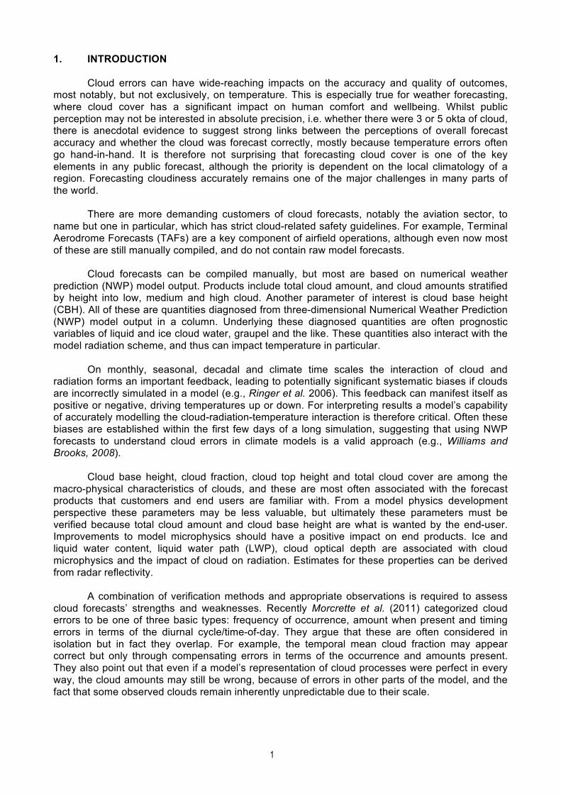
probability of the event could be used. For a more detailed discussion see Jolliffe and Stephenson (2003). Then the diagonal entries of the scoring matrix are given by:

,

with the off-diagonal elements are given by

Where and

_______

21

ANNEX B

Examples of Verification Methods and Measures B.1 Joint and marginal distributions

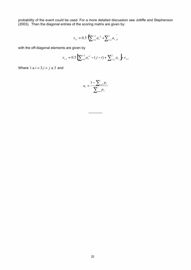
An example of a joint distribution of TCA against automated synoptic observations for the Met Office 1.5 km UKV model for 2010. Shown are the t+3h forecasts valid at 12Z.

Figure 1 - Example of the joint distribution (bottom left), and the two marginal distributions of forecast and observed TCA at 12Z during 2010. The legend top right refers to the shading of the joint distribution

22

B.2 Simple categorical statistics

At the Met Office the UK index, a corporate forecast accuracy benchmark, contains two cloud variables, total cloud amount (TCA) and cloud base height (CBH). It is evaluated using the Equitable Threat Score (ETS) for three categories each. The CBH height thresholds are set in line with requirements for civil and defence aviation. Figure 2 shows the >4 okta cloud and the <500m CBH ETS time series as a 36-month running mean value.

(a) (b)

Figure 2 - Example of simple 36-month running mean ETS components for one category of TCA (a) and one of CBH (b) to show the scores evolving over time and with forecast lead time

23

B.3 Multiple-category contingency tables

Multi-category contingency table of one year (with 19 missing cases) of cloudiness forecasts from the HIRLAM model are shown in Figure 3(a), with resulting statistics (b). Results are shown exclusively for forecasts of each cloud category, together with the overall values of Proportion Correct (PC), Kuipers Skill Score (KSS) and Heidke Skill Score (HSS). The most marked feature is the very strong over-forecasting of the “partly cloudy” category leading to numerous false alarms (Bias = 2.5, False Alarm Rate (FAR) = 0.8), and, despite this, the poor Probability of Detection (POD = 0.46). The forecasts did not reflect the observed U-shaped distribution of cloudiness. Regardless of this inferiority both overall skill scores are relatively high (~0.4), following the fact that most of the cases (90%) fall either in the “no cloud” or “cloudy” category - neither of these scores takes into account the relative sample probabilities, but weight all correct forecasts similarly.

(a) (b)

Figure 3 - Example of a multi-category contingency table from FMI

The Gerrity Score for this example is 0.455.

24

Figure 4 shows the data transformed into hit/miss bar charts, given the observations on the left, or the forecasts on the right. The green, yellow and red bars denote correct, one and two category errors, respectively. The U-shape in observations is clearly visible (left), whereas there is little hint of such in the forecast distribution (right).

Figure 4 - Hit-miss frequency bar chart for FMI statistics in Figure 2. The left-hand panel refers to the columns, and the right-hand panel to the rows

25

B.4 Continuous scores and parameters Figure 5 shows an example of verifying cloud parameters using continuous measures: the bias and standard deviation of cloud cover. (a) (b)

Figure 5 - Long time series of the bias and standard deviation of cloud cover from (a) the ECMWF deterministic forecasts and (b) the Unified Model 12-km mesoscale model to show different resolutions and forecast ranges

26

B.5 Verification of probabilistic MOS forecasts

The Meteorological Service Canada (MSC) runs operationally an updateable MOS, discriminant analysis-based probability forecast system for short range forecasts (0-48 h) of cloud amount in 4 categories. The forecasts are actually Bayesian probabilities, given the predictor values transformed to discriminant space to maximize separation of the 4 categories.

Results between the UMOS system are compared with an older perfect prog system, which used regression to predict the cloud amount in tenths. The verification statistics are calculated for the period between 2 January and 3 April 2003, for the 00Z model run. There are 104 stations for comparison at 09Z and 143 at 18Z.

Figure 6 - Categories for MOS output

The verification problem here was to fairly compare the probability forecasts with the categorical forecasts that came out of the PPM system. To do this the UMOS forecasts were transformed to categorical forecasts by choosing the category with the highest probability (UMOSbin) then the verification was redone. The RPS and RPSS were used (appropriate for multi-categories, and useable on probability or categorical forecasts) along with various scores from a 4 by 4 contingency table for the categorical forecasts. Of importance here was to get the distribution correct, which is a challenge when it is U-shaped, as cloud amount often tends to be. That is demonstrated by the frequency bias graphs.

27

Figure 7 - Biases for different data sets. Top left is at t+6h, bottom left t+12h, top right t+24h and bottom right t+48h

Figure 8 - A selection of scores for the Canadian cloud forecasts, plotted as a function of lead time (hours)

28

B.6 Reliability diagram

Figure 9 shows a reliability curve for step t+120h for cloud cover greater than 4/8. The blue dotted line is the sample climate and the numbers on the curve are the number of cases for each forecast bin. The relative forecast distribution is also shown.

Figure 9 - Reliability diagram for day 5 (t+120h) ECMWF cloud forecasts for cloud cover greater than 4 okta

29

B.7 ROC

ROC curves for the same threshold used in Figure 9 are shown in Figure 10. The symbols on the ROC diagram are the operational high resolution T799 model (filled symbol) and the T399 control forecast (unfilled symbol). To the side the likelihood diagram for non-occurrence (red) and occurrence (blue) as a function of forecast frequency is also provided. Ideally the two curves should not overlap, and have a maximum of either 0 (non-occurrence) or 1 (occurrence).

Figure 10 - ROC curves and likelihood diagrams for days 3 to 6 ECMWF forecasts for cloud cover greater than 4 okta

_______

30

ANNEX C

Overview of Model Cloud Validation Studies

Mittermaier (2012) reviewed the use of conventional synoptic observations for assessing TCA and CBH in four different model configurations, ranging from 1.5 km to 25 km. Skill scores for high-resolution NWP at the sub-2 km scale were found to be particularly disappointing. This is because high-resolution NWP models do not necessarily have the right detail in the right place at the right time, and are susceptible to the “double penalty” effect when using the traditional method of precise matching in space and time by using the nearest model grid box to an observing site. The study also showed that by considering a forecast neighbourhood centred on a point observation, and using a neighbourhood verification method, cloud scores improved by 1—5%, depending on the size of the neighbourhood and the fractional coverage. For coarser resolution models having multiple surface observations within the same model grid could lead to problems too. Gilleland (2004) discusses methods for thinning METAR data, recognizing that models may be awarded or penalized multiple times for correct or incorrect forecasts if many METAR data are located closely together.

Satellite data has been used extensively by model developers to validate cloud parameterization schemes in NWP models. The use of spatial verification methods has also been explored. Morcrette (1991) transformed cloudiness, temperature and humidity fields from the European Centre for Medium Range Weather Forecast model into brightness temperature fields that were compared to analogous brightness temperatures in the long wave window channel of Meteosat. Hodges and Thorncroft (1997) analyzed eight years of infrared International Satellite Cloud Climatology Project (ISCCP) satellite imagery applying an objective feature identification algorithm. The features (convective cells) were tracked and statistics of genesis, lysis, mean propagation and mean strength were studied for a summer period (June to September) for a region in Africa. Garand and Nadon (1998) used the model-to-satellite approach to compute radiances in order to compare forecasts of cloud fraction, height and outgoing radiation to near-coincident Advanced Very High Resolution (AVHRR) imagery. Chevalier et al. (2001) used the High-Resolution Infrared radiation Sounder/2 (HIRS/2) and the Microwave Sounding Unit (MSU) observations on board the National Oceanic and Atmospheric Administration (NOAA) satellites to assess forecasts of the European Centre for Medium Range Weather Forecast (ECMWF). Chaboureau et al. (2002) discuss the model-to-satellite approach for a direct comparison between simulated and observed cloud fields. Keil et al. (2003) compare synthetic satellite imagery from the mesoscale model of the Deutscher Wetterdienst with Meteosat-7 brightness temperatures. To take advantage of the high spatial resolution of the satellite observations, the data are projected onto the model grid with a simple remapping and at each grid point an average radiance of the satellite data within the grid box is calculated.

Jakob (2003) also looked at cloud verification from a modelling viewpoint, discussing the importance of establishing a strategy for cloud parameterization evaluation using both conventional and satellite data. Li and Weng (2004) used satellite-retrieved cloud products, like ice water path (IWP) or liquid water path (LWP), to validate cloud simulations in the National Centers for Environmental Prediction (NCEP) operational model. Most of them use information from models to convert radiances to variables like cloud cover, cloud top height and fog, which might make their use for verification purposes inappropriate, particularly in case of NWP model inter-comparisons since the observations are no longer independent of the model being verified. For example, if temperature and moisture fields from one model are used to convert from radiances to cloud cover, that model will have an unfair advantage over any other model in the same inter-comparison project. Chaboureau and Bechthold (2005) also produced synthetic brightness temperature corresponding to the GOES-E infrared channel-4 in the thermal infrared window for comparative purposes. Williams and Brooks (2008) used the ISCCP (International Satellite Cloud Climatology Project) data set of cloud optical depth and cloud top pressure to look at initial tendencies in cloud amounts to understand process errors in a global model.

31

Direct measurements of the vertical structure of the clouds were limited to a few ground-based radar sites such as those included in the Atmospheric Radiation Measurement (ARM) Programme, which brought together a range of active sensors to consider cloud properties, see, e.g., Clothiaux et al. (2000). Jakob et al. (2004) used radar and lidar measurements from ground-based stations in an idealized setting to move from a deterministic to a probabilistic model evaluation. The CloudNet project described by Illingworth et al. (2007) is a European example of the combined use of cloud radar, lidar and radiometer data for cloud assessment. This data set has been widely used for the verification of cloud in NWP models of different resolutions, e.g., Hogan et al. (2009), Bouniol et al. (2010), and Morcrette et al. (2011). All these studies represent a site-specific assessment which provides detailed analyses of the vertical structure and distribution of cloud-related model parameters. Böhme et al. (2011) produced a 2-year continuous evaluation of integrated water vapour, brightness temperature, cloud base height and precipitation.

Direct measurements of the vertical profile are now also available from active sensors on satellites, providing much wider coverage than just at a particular location. Stephens et al. (2002) describe the potential of CloudSat and the A-train. Mace et al. (2007) describe the early results from CloudSat Geometrical Profiling Project, which attempts to identify the location of hydrometeors in the earth’s atmosphere. Palm et al. (2005) have compared vertical profiles of the European Centre for Medium Range Weather Forecast model cloud fraction with backscatter data from the Geoscience Laser Altimeter System (GLAS) on ICESat by overlaying the model field onto the satellite images and making a visual qualitative assessment of the model performance. Bodas-Salcedo et al. (2008) compared simulated radar reflectivities against CloudSat radar reflectivities.

_______

32

ANNEX D

Contributing Authors

Marion Mittermaier, Met Office, United Kingdom

Anna Ghelli, European Centre for Medium-range Weather Forecasting (ECMWF), United Kingdom

Elizabeth Ebert, Bureau of Meteorology, Australia

Laurence Wilson, Environment Canada

Pertti Nurmi, Finnish Meteorological Institute

_______

33

World Weather Research Programme (WWRP) Report Series

Sixth WMO International Workshop on Tropical Cyclones (IWTC-VI), San Jose, Costa Rica, 21-30 November 2006 (WMO TD No. 1383) (WWRP 2007 - 1). Third WMO International Verification Workshop Emphasizing Training Aspects, ECMWF, Reading, UK, 29 January - 2 February 2007) (WMO TD No. 1391) (WWRP 2007 - 2). WMO International Training Workshop on Tropical Cyclone Disaster Reduction (Guangzhou, China, 26 - 31 March 2007) (WMO TD No. 1392) (WWRP 2007 - 3). Report of the WMO/CAS Working Group on Tropical Meteorology Research (Guangzhou, China, 22-24 March 2007) (WMO TD No. 1393) (WWRP 2007 - 4). Report of the First Session of the Joint Scientific Committee (JSC) for the World Weather Research Programme (WWRP), (Geneva, Switzerland, 23-25 April 2007) (WMO TD No. 1412) (WWRP 2007 – 5). Report of the CAS Working Group on Tropical Meteorology Research (Shenzhen, China, 12-16 December 2005) (WMO TD No. 1414) (WWRP 2007 – 6).

Preprints of Abstracts of Papers for the Fourth WMO International Workshop on Monsoons (IWM-IV) (Beijing, China, 20-25 October 2008) (WMO TD No. 1446) (WWRP 2008 – 1).

Proceedings of the Fourth WMO International Workshop on Monsoons (IWM-IV) (Beijing, China, 20-25 October 2008) (WMO TD No. 1447) (WWRP 2008 – 2). WMO Training Workshop on Operational Monsoon Research and Forecast Issues – Lecture Notes, Beijing, China, 24-25 October 2008 (WMO TD No. 1453) (WWRP 2008 – 3). Expert Meeting to Evaluate Skill of Tropical Cyclone Seasonal Forecasts (Boulder, Colorado, USA, 24-25 April 2008) (WMO TD No. 1455) (WWRP 2008 – 4). Recommendations for the Verification and Intercomparison of QPFS and PQPFS from Operational NWP Models – Revision 2 - October 2008 (WMO TD No. 1485) (WWRP 2009 - 1). Strategic Plan for the Implementation of WMO’s World Weather Research Programme (WWRP): 2009-2017 (WMO TD No. 1505) (WWRP 2009 – 2). 4th WMO International Verification Methods Workshop, Helsinki, Finland, 8-10 June 2009 (WMO TD No. 1540) (WWRP 2010 - 1). 1st WMO International Conference on Indian Ocean Tropical Cyclones and Climate Change, Muscat, Sultanate of Oman, 8-11 March 2009 (WMO TD No. 1541) (WWRP 2010 - 2). Training Workshop on Tropical Cyclone Forecasting WMO Typhoon Landfall Forecast Demonstration Project, Shanghai, China, 24-28 May 2010 (WMO TD No. 1547) (WWRP 2010 - 3) (CD only). 2nd WMO International Workshop on Tropical Cyclone Landfall Processes (IWTCLP-II), Shanghai, China, 19-23 October 2009 (WMO TD No. 1548) (WWRP 2010 - 4). 5th WMO Symposium on Data Assimilation, Melbourne, Australia, 5-9 October 2009 (WMO TD No. 1549) (WWRP 2010 - 5).

34

7th International Workshop on Tropical Cyclones (IWTC-VII), Saint-Gilles-Les-Bains, La Réunion, France, 15-20 November 2010 (WMO TD No. 1561) (WWRP 2011 – 1). Report of the Fourth Session of the Joint Scientific Committee (JSC) for the World Weather Research Programme (WWRP),Geneva, Switzerland, 21-24 February 2011, (WWRP 2011 - 2). WWRP/ETRP Workshop on Operational Monsoon Research and Forecast Issues – Lecture Notes, Beijing, China, 24-25 October 2008, (WWRP 2011 - 3).