1

1

2

3

Reconciling differences in Pool-GWAS between populations: a case study of 4

female abdominal pigmentation in Drosophila melanogaster 5

6

7

Lukas Endler1, Andrea J. Betancourt1, Viola Nolte1, and Christian Schlötterer1* 8

9

10

11

1Institut für Populationsgenetik , Vetmeduni Vienna, 1210 Wien, Austria 12

13

14

*Corresponding author 15

16

Data submitted to European Nucleotide Archive (ENA): 17

ERP001827 and ERP013300 18

19

Genetics: Early Online, published on December 29, 2015 as 10.1534/genetics.115.183376

Copyright 2015.

2

Running Title: Pool-GWAS in multiple populations 1

2

Key words: GWAS, Genome wide association study, pigmentation, dominance, 3

Drosophila melanogaster, pooled sequencing 4

5 Corresponding author: 6

Christian Schlötterer 7

Institut für Populationsgenetik 8

Vetmeduni Vienna 9

Veterinärplatz 1, 1210 Wien, Austria 10

E-mail: christian.schloetterer@vetmeduni.ac.at (CS) 11

Telephone: +43 1 25077-4300 12

13

14

15

3

1 Abstract 2

The degree of concordance between populations in the genetic architecture of a given 3

trait is an important issue in medical and evolutionary genetics. Here, we address this 4

problem, using a replicated pooled genome wide association approach (Pool-GWAS) 5

to compare the genetic basis of variation in abdominal pigmentation in female 6

European and South African Drosophila melanogaster. We find that, in both the 7

European and the South African flies, variants near the tan and bric-à-brac 1 (bab1) 8

genes are most strongly associated with pigmentation. However, the relative 9

contribution of these loci differs: in the European populations, tan outranks bab1, 10

while the converse is true for the South African flies. Using simulations, we show that 11

this result can be explained parsimoniously, without invoking different causal variants 12

between the populations, by a combination of frequency differences between the two 13

populations and dominance for the causal alleles at the bab1 locus. Our results 14

demonstrate the power of cost-effective, replicated Pool-GWAS to shed light on 15

differences in the genetic architecture of a given trait between populations. 16

17

Introduction 18

Insight into the genetic basis of phenotypic variation within species is essential 19

to understanding of short-term evolutionary change, as phenotypic variation is an 20

important substrate for natural selection. This endeavor has benefited from the steep 21

decrease in the cost of rapid genotyping techniques, including DNA sequencing, 22

which facilitates the mapping of traits using either genetic crosses (i.e., quantitative 23

trait mapping), or statistical association studies (i.e., genome-wide association studies, 24

or GWAS, reviewed in Visscher et al. 2012). As a result, it is now feasible to replicate 25

4

association studies in multiple samples. One question we can therefore address is 1

whether the same loci and alleles underlie phenotypic variation in different 2

populations of species with broad geographic distributions, or whether the alleles tend 3

to be population-specific. Human disease studies sometimes attempt to replicate the 4

results of genome-wide association studies in additional populations, with varying 5

success (e.g, Li et al. 2008; Ng et al. 2008; Siontis et al. 2010). Results for disease 6

traits, however, may not be representative of those for adaptive traits. Genetic 7

diseases are probably most often due to unconditionally deleterious alleles kept at low 8

frequency by purifying selection, and thus likely to be population specific due to their 9

rarity (Ioannidis et al. 2009, 2011; Gorlov et al. 2014). Data for adaptively varying 10

traits are sparser than those for diseases. The best-studied examples are lactase 11

persistence in humans, which is due to several independently derived alleles, the 12

frequency of which differs among geographic regions (Ingram et al. 2009; Itan et al. 13

2010; Ranciaro et al. 2014), and cryptic coat coloration in mice, for which the genetic 14

basis also differs between populations (Hoekstra and Nachman 2003; Hoekstra et al. 15

2006). 16

Here, we replicate a study of abdominal pigmentation in Drosophila 17

melanogaster (Bastide et al. 2013), originally done in two European populations, in a 18

geographically distant African population. Pigmentation in D. melanogaster is a 19

useful trait for this purpose for several reasons. For one, the underlying genetic 20

pathways are well-described, with most of the characterized genes playing a role in 21

either biochemical synthesis of the pigments, or in sexually dimorphic and spatial 22

regulation of the pigment-synthesis genes (Wittkopp et al. 2003; Gompel et al. 2005). 23

For another, this trait is both highly variable and highly heritable (Robertson et al. 24

1977; Gibert et al. 1998a; Pool and Aquadro 2007; Dembeck et al. 2015), with a 25

5

reasonably simple genetic basis, qualities which render the genetics underlying this 1

variation tractable to statistical analysis . Finally, spatial patterns of variation in this 2

trait suggest that it is ecologically important. In particular, both thoracic and 3

abdominal pigmentation patterns vary strongly with altitude and latitude (Telonis-4

Scott et al. 2011; David et al. 1985; Munjal et al. 1997; Pool and Aquadro 2007; 5

Capy et al. 1988), with independent clines found on different continents. In the 6

ancestral range in Africa, geographic variation is most strongly associated with levels 7

of UV-radiation, consistent with higher UV tolerance of darkly pigmented flies 8

compared to light ones (Bastide et al. 2014). 9

There have been several previous studies of pigmentation variation in 10

Drosophila, describing the genetic basis of variation in abdominal pigmentation 11

between species and between sexes (Llopart et al. 2002; Wittkopp et al. 2003; 12

Gompel et al. 2005; Jeong et al. 2006, 2008; Williams et al. 2008; Rogers et al. 2013; 13

Rogers et al. 2014; Salomone et al. 2013), and on variation in thoracic and abdominal 14

pigmentation within species (Robertson et al. 1977; Pool and Aquadro 2007; 15

Takahashi et al. 2007; Bickel et al. 2011; Takahashi and Takano-Shimizu 2011; 16

Bastide et al. 2013; Rogers et al. 2014; Dembeck et al. 2015; Wittkopp et al. 2010; 17

Cooley et al. 2012). The latter studies are the most relevant here. Thoracic 18

pigmentation phenotypes, including differences between African strains and variation 19

along a latitudinal cline, map to major effect loci near ebony, a pigment synthesis 20

gene (Takahashi et al. 2007; Telonis-Scott et al. 2011; Takahashi and Takano-21

Shimizu 2011). Abdominal pigmentation variation has a slightly more complex 22

genetic basis, and has been attributed to variants at three loci: bric-à-brac (bab), tan, 23

and ebony (Robertson et al. 1977; Kopp et al. 2003; Pool and Aquadro 2007; Bickel 24

et al. 2011; Bastide et al. 2013; Dembeck et al. 2015). All three of these loci have 25

6

well-described roles in pigmentation. Bab, which comprises two protein coding genes 1

(bab1 and bab2) is a spatial regulator of sexual dimorphic pigmentation at the tip of 2

the abdomen (Robertson et al. 1977; Kopp et al. 2000; Williams et al. 2008), and tan, 3

like ebony, is involved in pigment synthesis (True et al. 2005). Two independent 4

association studies have resulted in genome-wide, fine-resolution maps of 5

associations at these loci (Bastide et al. 2013; Dembeck et al. 2015). Both implicate 6

variants in cis-regulatory elements at tan, bab, and ebony, though the loci with the 7

largest effect varied between studies. In the Bastide et al. 2013 study, the variants 8

with the strongest effect lay upstream of the tan gene, in a cis-regulatory element 9

called the male specific enhancer (MSE). The MSE has also been implicated in the 10

pigmentation differences between D. santomea and D. yakuba (Jeong et al. 2008). 11

Variants in a regulatory element of bab1 (the dimorphic element, or DME), played a 12

significant, but minor role, and those upstream of ebony were of borderline 13

significance. Dembeck et al. (2015), in contrast, found the bab locus had a major 14

effect on pigmentation variation, while tan and ebony and other loci had minor 15

effects. 16

In this study, we replicate the Bastide et al. (2013) study in a South African 17

population of D. melanogaster, using the Pool-GWAS approach, but with some 18

important modifications. Although we find that same variants appear to be causal in 19

both populations, bab, rather than tan, shows the strongest association with 20

pigmentation in the South African population, similar to results from the Dembeck et 21

al. (2015) study and in contrast to the Bastide et al. (2013) study. We analyze these 22

results in detail to explain the reasons for the contrasting genetic associations between 23

the South African and European populations. 24

7

Results and Discussion 1

Variation within and between samples: We used samples of D. 2

melanogaster from three locations for this study. After adding an additional replicate 3

for the Viennese population, we reanalyzed the population samples from Bastide et al. 4

(2013), which consisted of two European populations, from near Bolzano, Italy, and 5

Vienna, Austria, about 200 miles apart. We also collected and analyzed data from a 6

new population, from Kanonkop, near Cape Town, South Africa. We divided each of 7

the three population samples into three replicates, which were then scored for female 8

abdominal pigmentation. Within each replicate, we identified individuals with 9

extreme phenotypes — those with the greatest and least extent of darkly pigmented 10

area on segment A7, as in Bastide et al. (2013) — pooled them, and subjected the 11

pools of light and dark individuals from each replicate to whole genome sequencing 12

(see Table S1 for coverage depth). We then analyzed these pools for allele frequency 13

differences that suggest an association with the pigmentation phenotype. The six 14

replicates from the European populations consisted of 1500 offspring of wild-caught 15

females, with 100 individuals (~7%) per replicate contributing to each extreme pool. 16

The South African samples, for logistical reasons, were kept as 700 isofemale lines 17

for 15 generations before they were scored for pigmentation. Each of the three 18

replicates from this sample consisted of a single individual sampled from each 19

isofemale line, with a similar fraction of the individuals contributing to the extreme 20

pools as in the European populations (55-80 females, or 7-11% of each replicate). 21

After mapping and filtering, we identified ~3.2 million single nucleotide 22

polymorphisms (SNPs) segregating in the European population and ~4 million SNPs 23

in the South African isofemale lines with ~1.9 million common to both. The SNPs 24

shared by both populations had significantly higher minor allele frequencies (MAF) 25

8

than the SNPs found in only one of the two populations (shared SNPs: median MAF 1

EU and SA: 0.12, private SNPs: median MAF EU: 0.006, SA: 0.015; paired Wilcoxon 2

rank sum test EU: W= 1e+12, p < 2.2e-16, SA: W= 3.5e+12, p < 2.2e-16). To estimate 3

divergence between the populations, we calculated pairwise FST values for 200kb 4

windows using PoPoolation2 (Kofler et al. 2011b). As differentiation between the 5

Austrian and Italian populations was low (median FST = 0.0107, 95% CI: [0.0105, 6

0.011]), we combined these samples for subsequent analysis, as in Bastide et al. 7

(2013). The South African sample showed higher, but still moderate, levels of 8

divergence from the European populations [median FST(Aut/SA) = 0.044 (95% CI: 9

[0.043, 0.046]), median FST(Ita/SA) = 0. 040 (95% CI: [0.039, 0.041])], lower than 10

those typically reported for comparisons between European and other African D. 11

melanogaster samples (FST ~ 0.20; Pool et al. 2012). The low levels of population 12

differentiation between Europe and South Africa seen here are probably at least 13

partially due to high levels of migration from cosmopolitan flies, shown to occur in 14

many African populations (Pool and Aquadro 2006), but which may be particularly 15

high for our South African sample due to Cape Town’s status as a shipping port. 16

For the South African population, we used flies from recently established 17

isofemale lines, which have a higher degree of inbreeding than the wild-derived F1s 18

used in the European study. As inbreeding in the South African samples may affect 19

the GWAS results, we first estimated the degree of inbreeding in these lines. To this 20

end, we sequenced 12 individual females from different isofemale lines and compared 21

these to 12 resequenced individual flies from the population collected in Bolzano, 22

Italy. In the South African flies, the median inbreeding coefficient, FIT, is 0.35 (95% 23

CI = [0.337, 0.361]) see Figure S1). This level of inbreeding can be explained by an 24

initial bottleneck of 2 progenitor flies and 15 generations at an effective population 25

9

size (Ne) of around 10-25, consistent with the conditions under which the isofemale 1

lines were propagated. FIT varied moderately but significantly among chromosomes, 2

with 2L and 3L showing the lowest inbreeding (median FIT= 0.28 both) and X and 2R 3

the highest (median FIT=0.43 and 0.5 respectively; Dunn’s test with Benjamin-4

Hochberg correction, comparison: 2L:3L and 2R:X p > 0.05, all other comparisons: p 5

< 10-6). In contrast, resequenced individual flies from the European populations, 6

which have not been maintained as isofemale lines, show little evidence of inbreeding 7

(median FIT ≈ 0.00, 95% CI: [-0.009, 0.001]), as expected for flies with essentially the 8

same genotypes as wild flies. 9

SNPs associated with variation in abdominal pigmentation: To find SNPs 10

associated with abdominal pigmentation, we compared the allele frequencies of the 11

extreme light and dark pools of the European and South African populations across 12

replicates using the Cochran-Mantel-Haenszel (CMH) test as in Bastide et al. (2013). 13

In both populations, most of the 100 highest ranked SNPs (ranked by p-value from the 14

CMH test) are located in non-coding regions – 73% in the European population, and 15

95% in the South African one (see Tables S2-S7). Nevertheless, in the European 16

population, the highly ranked SNPs are enriched for those in coding regions compared 17

to random samples matched in size, chromosomal distribution, and allele frequency 18

(100,000 samples: p < 10-4). This enrichment is, however, mostly due to the overlap 19

of the tan regulatory region with the coding sequence of various flanking genes (14 20

synonymous and 5 non-synonymous SNPs). 21

In general, the results for the European population (Figure 1) are essentially 22

the same as in Bastide et al. (2013), with minor differences likely due to the inclusion 23

of an additional replicate for the Viennese population and a slightly altered SNP 24

calling and filtering protocol. The strongest associations are due to SNPs found 25

10

upstream of the tan locus, with the highest-ranking SNPs in the MSE region (Figure 1

1A,C, Table S3, S6, S7). The remaining strongly associated SNPs are near the bric-a-2

brac locus (hereafter called bab), and weakly associated SNPs occur upstream of the 3

ebony gene on 3R and close to the pdm3 gene on 2R. While only weakly associated 4

with pigmentation, it is plausible that both ebony and pdm3 are causal, as both have 5

been implicated in abdominal pigmentation in other studies (Pool and Aquadro 2007; 6

Rogers et al. 2014). 7

In contrast, in the South African sample (Figure 1B, Table S2, S4, S5), the 8

SNPs with the strongest associations occur at bab, not tan. Specifically, these SNPs 9

lie in the third intron of bab1, near a cis-regulatory region called the dimorphic 10

element (Figure 1D; Williams et al. 2008). The next strongest associations were with 11

SNPs at the tan locus. The change in ranks for the tan and bab loci between Europe 12

and South Africa is investigated in detail below. Finally, we again found SNPs 13

weakly associated with pigmentation at the pdm3 locus, as in the European sample, 14

but none near the ebony locus (Figure 1, Figures S2 & S3). 15

Using D. simulans as an outgroup, we inferred the ancestral states of the 16

strongly associated SNPs via parsimony. Interestingly, the inferred ancestral 17

phenotype differs at the tan and bab loci: For tan, most of the ten highest ranking 18

SNPs with a consistent effect in both samples had an inferred ancestral light allele 19

(Eu: 7/10, SA: 9/10). At the bab locus, in contrast, the majority of SNPs had an 20

ancestral dark allele. (Eu: 8/10, SA: 7/10; Tables S2 and S3). 21

Non-SNP variants associated with abdominal pigmentation: Strongly 22

associated SNPs may not directly cause abdominal pigmentation differences, but may 23

instead be associated with pigmentation via linkage to causal alleles consisting of 24

other kinds of genetic variation, namely, short insertion and deletion (indel) variants, 25

11

and large chromosomal inversions. To investigate these data for differences in indel 1

frequencies between the pools, we identified 279,016 segregating short insertions and 2

deletions in one of the European pools and 371,146 in the South African samples, 3

with 199,676 of these segregating in all populations (with the requirement that they 4

segregate with a minor allele frequencies of at least 15%). As with the SNPs, we 5

compared allele counts of the indels in the extreme pools over replicates using a CMH 6

test. While indels and SNPs could, in principle, be combined and analyzed together, 7

we examined the indel results separately. The reason is that the indel allele counts are 8

likely less reliable than the SNP allele counts, as calling indels is technically difficult 9

compared to identifying SNPs, especially in pooled sequencing samples. 10

Overall, we find patterns similar to those obtained with SNPs (Figures S4 and 11

S5). For the European samples, highly associated indels are found around the same 12

regions close to tan and bab1, while for the South African flies, the only strongly 13

associated indels were near bab1, with none near the tan locus. In general, indels 14

associated with pigmentation variation showed higher p-values and smaller average 15

allele frequency changes than the highly associated SNPs (median of the log(OR) of 16

the 10 most significant variants: Eu: SNPs=1.8, indels=1.3; SA: SNPs=2.1, 17

indels=1.7), suggesting that the observed phenotypic variation is more likely to be due 18

to the SNPs than the indels. 19

We further investigated the pools of light and dark flies for differences in the 20

frequencies of cosmopolitan inversions. The inversions themselves are unlikely to 21

cause pigmentation differences, but as they suppress recombination in heterozygotes, 22

any causal variants contained in the inverted type may be linked to many other 23

variants also associated with the inversion. To investigate this possibility, we looked 24

for differences in the frequencies of six common cosmopolitan inversions on 25

12

chromosomes 2 and 3 between the light and dark pools. We identified inversion types 1

indirectly, via previously identified SNP markers from Kapun et al. (2013). 2

While some inversions showed considerable frequency differences between 3

light and dark pools in the European populations (Figure S6), these differences were 4

not consistent between the Italian and Austrian samples, and were not replicated in the 5

South African pools. Thus, these frequency differences may lead to an overall 6

elevation in allele frequency differences between the pools, but, assuming that the 7

inversions are associated with similar alleles in both European samples, they are 8

unlikely to lead to consistently associated alleles even in the European samples. In 9

addition, linkage disequilibrium between alleles and inversions is likely strongest at 10

the inversion breakpoints (Andolfatto et al. 1999). The closest inversion breakpoint of 11

any of the investigated inversion is ~2MB away from the bab locus, possibly close 12

enough to affect allele frequencies (Stevison et al. 2011), but unlikely to result in 13

strong spurious association at bab and not elsewhere on 3L. The tan locus is X-linked, 14

and the X-chromosome harbors no known common inversions (Lemeunier and Aulard 15

1992). In any case, the inversions are unlikely to cause artifactual signals at tan and 16

bab. 17

Similarities and differences between the populations: We noted several 18

differences between the European and South African populations. In particular, the 19

weak effect of ebony is restricted to the European population, and the strongest 20

signals occur near tan in the European population, but near bab in the South African 21

population. Nevertheless, we identified similar sets of genes overall in the two 22

populations, raising the question as to whether pigmentation is affected by the same 23

alleles in the two populations, or by independent alleles at the same loci. We tested 24

this by asking if highly ranked SNPs (ranked separately by significance for each 25

13

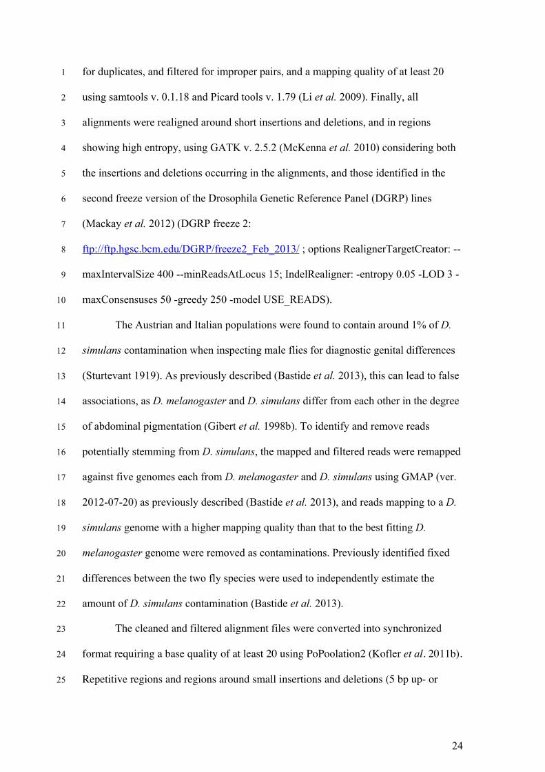
population) had consistent effects in the two samples, using two different measures of 1

consistency. First, we asked the alleles at these SNPs had the same qualitative effect 2

for Europe and South Africa, assuming that the ‘dark’ allele at each SNP is that 3

enriched in the dark sample of flies (and vice-versa). For unassociated diallelic SNPs, 4

we expect half of them to have the same qualitative effect in the two samples. High-5

ranking SNPs, however, have the same inferred dark and light alleles much more 6

often than this (Figure 2A). Second, we asked if high-ranking SNPs in one population 7

had the strongest estimated phenotypic effects in the other population, as expected. 8

We estimated and ranked phenotypic effects using the logOR for dark vs. light pools 9

(Bastide et al. 2013; Figures S7 and S8). The results again show broad consistency 10

between the populations; in particular, high-ranking SNPs in Europe generally had the 11

highest ranked phenotypic effects in South Africa (Figure 2B). For both measures of 12

similarity, the concordance between the samples declines steeply as the effects of 13

highly ranked SNPs are diluted by SNPs with increasingly lower ranks (Figure 2). 14

Overall, we conclude that despite the striking differences between the populations, 15

this analysis suggests that some SNPs contribute similarly to female abdominal 16

pigmentation in both populations. Otherwise, we would not expect to find consistency 17

between the high-ranking SNPs of the two populations, as each would contain two 18

different sets of causal variants and linked SNPs. 19

That said, the ranks of the highest-ranking South African SNPs were poor 20

predictors of the ranks of their effect sizes in Europe compared to the reciprocal 21

comparison (Figure 2). Inspection of the data reveals that this discrepancy arises 22

mainly from the region near bab1, where some SNPs were high ranking in South 23

Africa, but not in Europe. Tellingly, these SNPs segregate at intermediate frequencies 24

in South Africa, and at low frequencies in Europe [median minor allele frequencies 25

14

(MAF) of the 50 highest ranked SNPs in South Africa = 0.42, median MAF in Europe 1

= 0.26; paired Wilcox rank-sum test p = 0.0004]. The logOR estimator is akin to the 2

average effect of an allelic substitution (Falconer and Mackay 1996), in that it is 3

affected in a similar way by dominance and allele frequency. That is, in the absence 4

of dominance, the logOR effect estimates are affected very little by differences in 5

allele frequencies (Figure S7A). With dominance though, logOR estimates do change 6

with allele frequency, reflecting the change in the proportion of individuals expressing 7

the full homozygous effects of the recessive allele (Figure S7B). Thus, the failure to 8

observe a strong effect for the bab1 SNPs in Europe might be explained by a lower 9

MAF of the recessive allele, so that its effects are rarely expressed and such that it 10

contributes little to phenotypic variation in Europe. At the tan gene, in contrast, the 50 11

highest ranked SNPs in the South African sample had comparable median MAFs in 12

reference samples from both populations (median MAF Europe: 0.75, SA: 0.70; 13

paired Wilcox rank-sum test p = 0.99; Figure S9), and the effects for these SNPs were 14

more consistent than for those at the bab locus. 15

Refining candidates using the combined analysis of multiple populations: 16

Despite the high resolution of Pool-GWAS, for closely linked sites, several alleles 17

from a single population are associated with a causal variant via linkage 18

disequilibrium, resulting in false positives. The combined analysis of multiple 19

populations may make use of more historical recombination events than have 20

occurred in a single population. As a result, provided that the genetic architecture of 21

the trait is identical among the populations, their joint analysis can yield fewer false 22

positives and higher confidence candidates than the analysis of a single population. 23

Considering only high ranking SNPs with consistent effects in the two populations, 24

15

for example, we can narrow down the SNPs at bab to a single best candidate SNP 1

(3L:1085454 at bab1). 2

For SNPs in very close proximity, we can use patterns of linkage to further 3

refine the location of SNPs that show consistent changes between populations. We 4

achieve this by using information from SNPs on the same read or read pair, and 5

estimating short-range linkage disequilibrium between the associated SNPs as in 6

Feder et al. (2012). We combined pairs of SNPs with estimated r2 values > 0.75 to 7

infer short haplotypes. We then determined the frequency changes and the associated 8

p-values of SNPs associated with these haplotypes (Figures S9-S11) to determine 9

whether candidate SNPs increase in frequency independently of nearby SNPs, or as 10

part of a haplotype. For example, the three most highly ranked tan SNPs in the 11

European population appear to occur primarily on the same haplotype, consistent with 12

their close physical distance (e.g,, the two most tightly linked SNPs, X:9121094 and 13

X:9121129, show r2(EU)~0.97, r2(SA)~0.83). Unfortunately, this does not implicate a 14

single best candidate SNP, as the response of all three SNPs is likely non-15

independent. In contrast, the analysis of three groups of SNPs upstream of the tan 16

gene (X:9119116-9119160,9120730&912683, 9123892-9123903) demonstrates the 17

usefulness of this approach. In the analysis of the European population, the SNPs 18

within a group show strong linkage disequilibrium resulting in almost identical allele 19

frequency change. In the South African population, these alleles do not show the same 20

pattern of linkage disequilibrium, and only one SNP in each of the groups exhibits 21

consistent allele frequency changes in the South African sample. yielding a single best 22

candidate causal allele for each of the three haplotypes (see green boxes in Figure 23

S10). 24

16

Contrasts between populations at the tan and bab loci: We used 1

simulations to ask if we can simply explain the contrasting effects of effects of tan 2

and bab in Europe and South Africa, assuming a identical genetic architecture of 3

causal loci underlying the phenotype. Specifically, we investigated the role of 4

dominance and allele frequency differences between the populations. We simulated as 5

closely as possible the actual Pool-GWAS procedure for both populations, using the 6

same number of sequenced individuals and replicates, and estimated allele 7

frequencies from the European and South African reference populations (median 8

frequency for the light allele of the 4 best candidates at each locus: Europe: tan: 0.2, 9

bab: 0.83; SA: tan: 0.17, bab: 0.47, see Table 1). We assigned genotypes to 10

individuals based on these allele frequencies, accounting for inbreeding in the South 11

African population (using FIT = 0.35), and phenotypes based on these genotypes, 12

assuming a narrow-sense heritability (h2) of 0.3. This value is conservative compared 13

to the typical estimate of h2 = 0.5 to 0.9 for abdominal pigmentation (Bickel et al. 14

2011; Dembeck et al. 2015), allowing for the effects of background loci. We assigned 15

the same mean phenotype to individuals with the same genotype, regardless of 16

population. As in the real experiment, simulated individuals were divided into 17

replicates, selected for their phenotypes, and their pooled allele counts analyzed with 18

a CMH test. 19

In the simulations, we varied the degree of dominance (h) of the light allele at 20

each locus and the relative additive effect sizes between the two loci (E), and then 21

accepted the 1% of simulations best fitting the following four criteria: the ratio of 22

effects of tan and bab in (i) Europe (actual results, tan-logOR/bab-logOR = 2.51) and 23

(ii) South Africa (tan-logOR/bab-logOR = 0.57), and the ratio of effects of these 24

SNPs across populations (iii) tan [Europe-logOR/South Africa-logOR = 1.89 and for 25

17

(iv) bab (Europe-logOR/South Africa-logOR = 0.44, see Table 1). Additional details 1

of the simulation methods are given in the Methods. The results of rejection sampling 2

are shown in Figure 3, S12 and S13. These most probable parameter combinations 3

had dominant light alleles at both bab (consistent with Robertson et al. 1977), and 4

tan, and a stronger effect of bab vs. tan alleles. Nearly all accepted parameter 5

combinations (92%) resulted in switching of the ranks of tan and bab for the 6

European and South African populations. 7

To explore potential genetic interactions between the two loci, as suggested by 8

the results of Robertson et al. (1977), we also considered a model with a simple 9

epistatic interaction term (see Methods), allowing for synergistic (positive) or 10

antagonistic (negative) effects of the light allele. Including a positive epistatic 11

interaction between light alleles at the two loci substantially improves the model fit 12

(Bayes Factor: P(Data|Model with epistasis)/ P(Data|Model without epistasis) = 644; 13

Csilléry et al. 2012). However, as other factors, such as subtle differences in 14

experimental methods or differences between the populations at other causal loci, may 15

yield a similar effect, we do not consider this analysis strong evidence for epistasis. In 16

any case, the main results remain qualitatively unchanged: Similar to the model 17

without epistasis, this model also suggests dominance of the light alleles of both tan 18

and bab, though support for tan dominance is reduced, and a stronger allelic effect of 19

variants at the bab locus than at tan (Figures S14-S16). 20

Overall, our simulations suggest that the contrasting results between the 21

European and South African population can be at least partly explained by dominance 22

and allele frequency differences between the populations: As the dark allele at bab is 23

at high frequency in the South African population, the recessive homozygote is easily 24

recovered even in the absence of inbreeding. In contrast, the recessive homozygote in 25

18

Europe is rare (at an expected frequency of 2.9%), reducing its effect on phenotypic 1

variation and in the experiment, in spite of its large allelic effect. 2

Comparison of the results with previous studies: We compared the results 3

of our approach to two studies on natural genetic variation of female abdominal 4

pigmentation. For this analysis, we chose to maximize the chance of overlap with the 5

other two studies with a more liberal cutoff than the 5% FDR used for the main 6

results, instead using the 1019 SNPs with p-values below the Bonferroni threshold (p 7

= 1.56e-8 for Europe and p = 1.25e-8 for South Africa). We then looked for overlaps 8

between these SNPs and those identified as candidates in the other studies. 9

The first study, Bickel et al. (2011), investigated variants at the bric-à-brac 10

locus (bab1 and 2) segregating in a sample of 96 inbred lines from an orchard near 11

Winters, CA, USA, for their effects on A6 pigmentation. While this study measured 12

pigmentation for a different tergite, genotypic values for A6 and A7 are strongly 13

correlated (Gibert et al. 1998b), so an overlap between alleles affecting these traits 14

seems plausible. In the 148kb region covered by Bickel et al. 2011, there were 3066 15

uniquely mappable biallelic SNPs with a minor allele frequency ≥ 0.05; of these, 2367 16

were segregating in at least one of the populations used in this study, and 167 of these 17

2367 were identified as candidates by Bickel et al. 2011. Of these SNPs, 15 and 2 18

were significant after Bonferroni correction for multiple testing in the South African 19

and European studies, respectively (Table S8), including the most strongly associated 20

ones at the bab locus in the South African (3L:1084990) and the European 21

(3L:1085454) samples. The overlapping SNPs fall into two regions, the regulatory 22

region in the first intron of bab1, and the noncoding intergenic region between bab1 23

and bab2, ~50kb apart, much further than the usual extent of linkage disequilibrium in 24

19

D. melanogaster (Mackay et al. 2012; Franssen et al. 2015), suggesting that both 1

regions may affect pigmentation variation independently. 2

The second study, Dembeck et al. (2015), looked genome-wide for variants 3

associated with pigmentation of the 5th and 6th abdominal tergites (A5 and A6) of 4

females in a panel of 175 inbred and sequenced lines created from a population at 5

Raleigh, NC, USA (Mackay et al. 2012). We looked for overlap between our 1019 6

SNPs, and the 154 variants with a p-value below 1 x 10-5 in Dembeck et al. (2015) 7

associated with effects on either or both segments. In all, we found 15 candidate SNPs 8

in common between Dembeck et al. (2015) and this study; of these, 11 are in the first 9

intron of bab1 and 4 near the MSE upstream of tan (see Table S9). Encouragingly, the 10

inferred light and dark alleles for the SNPs affecting A7 (present study) and those 11

significantly affecting A6 (8 SNPs) or A5 (3 SNPs, with 2 of them also affecting A6) 12

in Dembeck et al. (2015) were identical between the studies, consistent with similar 13

associations and with correlated trait values for these segments (Gibert et al. 1998b). 14

The remaining 6 of the 15 SNPs had a complex effect on pigmentation, affecting the 15

contrast between the A5 and A6 segments—e.g., at these SNPs, alleles that increase 16

pigmentation in A6, reduce it for A5. As pigmentation of adjacent segments is more 17

strongly correlated than that of more distant ones (Gibert et al. 1998b), we expect the 18

effect of these alleles on A6, rather than that on A5, to predict the effect the A7 19

segment measured here. Consistent with this, the inferred light and dark alleles for all 20

six SNPs were identical for the A6 segment in Dembeck et al. (2015) and for A7 in 21

the present study. 22

We next asked whether the 15 SNPs that overlap between this study and the 23

Dembeck et al. 2015 study show quantitatively similar effects, again using log(OR) as 24

a proxy for effect size in our study, and focusing on the effect on A6 in the Dembeck 25

20

et al. (2015) study. For the European population, we found no correlation, perhaps not 1

surprisingly as the strongest associations occurred at different loci in this comparison. 2

For the South African population, where the strongest associations were near the same 3

locus (i.e, near bab), the estimated effects of the alleles were strongly correlated 4

(Spearman’s ρ = 0.86, p = 0.0013). 5

We did not find any signs of association around the other genes identified to 6

influence pigmentation in Dembeck et al. (2015), possibly due to differences in the 7

trait measured (A6 vs. A7 pigmentation), or due to other differences in the 8

methodology and power of these approaches. Finally, only one SNP– the most highly 9

associated one in bab1 for South Africa (3L:1084990)– overlapped between all three 10

studies (Bickel et al. 2011, Dembeck et al. 2015, and this study). 11

Conclusions:. Using the Pool-GWAS method on three different D. 12

melanogaster populations, we show that variants at tan and bab are associated with 13

female abdominal pigmentation variation. In addition to the strong statistical support 14

from the current study, our results are also supported by other studies on pigmentation 15

variation (Robertson et al. 1977; Kopp et al. 2003; Bastide et al. 2013; Dembeck et 16

al. 2015), and by forward genetic studies showing that both tan and bab affect 17

pigmentation when mutated. While the results for the South African and European 18

populations are broadly consistent, the differences between them are potentially 19

informative. The European study points to a large effect of tan, while the results from 20

the South African population (and other studies on natural variants; Robertson et al. 21

1977; Dembeck et al. 2015) attribute the strongest effects to bab. We show that this 22

difference does not necessarily reflect alternative genetic architectures, but can be 23

most simply explained by a combination of dominance and allele frequency: e.g, in 24

South Africa, the dark allele of bab, which appears to have a strong effect (present 25

21

study and Robertson et al. 1977; Kopp et al. 2003; Dembeck et al. 2015), is at high 1

enough frequency to occur in homozygous form reasonably often, and thus can 2

contribute substantially to phenotypic variation even if recessive. In Europe, in 3

contrast, the dark bab allele is rare, and, if recessive, contributes little to phenotypic 4

variation in wild flies. Regardless of its status in natural populations, a recessive bab 5

allele can play a large role in differences between inbred lines selected for extreme 6

phenotypes, as shown in previous studies (Robertson et al. 1977; Kopp et al. 2003). 7

Further, because distant populations may show different patterns of linkage 8

disequilibrium, studying associations in different populations provides a means to 9

help distinguishing linked but non-causal variants from causal alleles contributing to 10

the phenotype — e.g, a SNP that is significant for one sample may show no 11

association in another sample, or have different inferred ‘dark’ and ‘light’ alleles 12

between samples. Thus, by looking for associations that are repeatable across 13

populations, repeated association studies allow further fine-mapping of potential 14

causal alleles. 15

Finally, we also show that Pool-GWAS can be used to analyze inbred 16

individuals from isofemale lines, a common tool in population genetics (David et al. 17

2005), offering a cost effective way to study the genetic basis of phenotypic variation, 18

including obtaining reasonable estimates of relative effect sizes for different loci. That 19

this modified experimental design yields reliable results is important for logistical 20

reasons, as it allows collection and phenotypic measurement of samples to be 21

separated in time, such that the latter can be done under controlled laboratory 22

conditions. 23

22

Materials and Methods 1

Sample collection, iso-female lines used, and pigmentation scoring: For the 2

European populations around 30,000 flies were collected in Vienna, Austria, in 2010 3

and in Bolzano, Italy, in 2011, and split into replicates and used to create an F1 4

generation in the laboratory under 25ºC and scored for pigmentation as described in 5

Bastide et al. (2013). Briefly, offspring were kept at 18ºC for a few days post-eclosion 6

to allow adult pigmentation pattern to develop and stabilize. Pigmentation was scored 7

by visually classifying each individual according to the extent of darkly pigmented 8

area on the most posterior abdominal segment (A7 tergite). For classification five 9

levels of pigmentation ranging from 0 (not pigmented) to 4 (completely pigmented) 10

were assigned, and 100 individuals with the lightest and darkest levels (0 and 4, 11

respectively) of each replicate were randomly chosen for pool sequencing. Around 12

1500 individuals were scored for each replicate. As a control three replicates of 100-13

160 individuals not selected for abdominal pigmentation were used. 14

The South African population consisted of 700 isofemale lines collected in March 15

2012 in Kanonkop, SA. These isofemale lines were kept at 25ºC and the offspring left 16

for several days to allow for the adult pigmentation to mature and fully develop. For 17

each replicate one female individual was taken from each isofemale line, leading to a 18

replicate size of 700 individuals. The individuals were then visually scored for 19

pigmentation of their A7 tergite, and the 135 lightest and 173 darkest flies from each 20

replicate pooled and sequenced (19.3% and 24.7%, respectively). The average allele 21

frequencies in the Kanonkop population were estimated from pooled females obtained 22

from a subset of 564 isofemale lines. 23

DNA extraction, library preparation and sequencing: DNA from pooled and 24

individual flies was extracted following a modified high salt protocol (Miller et al. 25

23

1988) and fragmented using a Covaris S2 device (Covaris, Inc. Woburn, MA, USA). 1

Paired-end library preparation was based on the NEBNext® DNA Library Prep 2

Master Mix Set (E6040L, New England Biolabs, Ipswich, MA) for the pooled South 3

African sample and the individually sequenced Viennese flies, whereas a modified 4

protocol of the NEBNext® Ultra DNA Library Prep Kit (E7370L) was used for the 5

individually sequenced South African flies. Size selection and final library 6

purification were performed using AMPureXP beads (Beckman Coulter, CA, USA) 7

with an additional gel-based size selection for the pooled South African sample and 8

the individually sequenced Viennese flies. The resulting insert sizes were 400bp for 9

these two samples and approximately 550bp for the individual South African libraries. 10

For amplification of individually barcoded libraries, the PCR mastermix included in 11

the TruSeq DNA LT Sample Prep Kit (FC-121-2001, Illumina, San Diego, CA) or 12

Phusion Polymerase (NEB) and 12 PCR cycles were used. All libraries were 13

sequenced on a HiSeq2000 following a 2x100bp protocol. 14

Read Mapping, Filtering of Contaminants, Realignment: Sequencing reads 15

were trimmed, mapped to a reference genome using a Hadoop based distributed 16

computation framework and filtered as previously described (Kofler et al. 2011a; 17

Pandey and Schlötterer 2013; Bastide et al. 2013). Shortly, the reads were trimmed 18

using PoPoolation and a base quality threshold of 18 (Kofler et al. 2011a), and 19

mapped to the combined genomes of D. melanogaster (v. 5.18), Wolbachia pipientis 20

(AE017196.1), Lactobacillus brevis (CP000416.1), Acetobacter pasteurianus 21

(AP011170), and phage phiX174 (NC_001422.1) using BWA aln v. 0.5.9 (Li and 22

Durbin 2009) without seeding allowing for two gap openings (-o 2), an alignment 23

distance threshold leading to loss of less than 1% of reads assuming a 2% error rate (-24

n 0.01), and up to 12bp gap extensions (-e 12 –d 12). The aligned reads were checked 25

24

for duplicates, and filtered for improper pairs, and a mapping quality of at least 20 1

using samtools v. 0.1.18 and Picard tools v. 1.79 (Li et al. 2009). Finally, all 2

alignments were realigned around short insertions and deletions, and in regions 3

showing high entropy, using GATK v. 2.5.2 (McKenna et al. 2010) considering both 4

the insertions and deletions occurring in the alignments, and those identified in the 5

second freeze version of the Drosophila Genetic Reference Panel (DGRP) lines 6

(Mackay et al. 2012) (DGRP freeze 2: 7

ftp://ftp.hgsc.bcm.edu/DGRP/freeze2_Feb_2013/ ; options RealignerTargetCreator: --8

maxIntervalSize 400 --minReadsAtLocus 15; IndelRealigner: -entropy 0.05 -LOD 3 -9

maxConsensuses 50 -greedy 250 -model USE_READS). 10

The Austrian and Italian populations were found to contain around 1% of D. 11

simulans contamination when inspecting male flies for diagnostic genital differences 12

(Sturtevant 1919). As previously described (Bastide et al. 2013), this can lead to false 13

associations, as D. melanogaster and D. simulans differ from each other in the degree 14

of abdominal pigmentation (Gibert et al. 1998b). To identify and remove reads 15

potentially stemming from D. simulans, the mapped and filtered reads were remapped 16

against five genomes each from D. melanogaster and D. simulans using GMAP (ver. 17

2012-07-20) as previously described (Bastide et al. 2013), and reads mapping to a D. 18

simulans genome with a higher mapping quality than that to the best fitting D. 19

melanogaster genome were removed as contaminations. Previously identified fixed 20

differences between the two fly species were used to independently estimate the 21

amount of D. simulans contamination (Bastide et al. 2013). 22

The cleaned and filtered alignment files were converted into synchronized 23

format requiring a base quality of at least 20 using PoPoolation2 (Kofler et al. 2011b). 24

Repetitive regions and regions around small insertions and deletions (5 bp up- or 25

25

downstream) were removed. RepeatMasker (ver. 3.2.8, www.repeatmasker.org) was 1

used for identifying repetitive regions without considering low complexity regions 2

(option -nolow). Overall, after all filtering steps, an average sequencing depth of 3

around 100 was obtained, with coverages ranging from 27 to 278 (for details see 4

Table S2). 5

Association Mapping and False Detection Rate Calculation: To test for 6

associations of variants with abdominal pigmentation we used a Cochran-Mantel-7

Haenszel (CMH) test as previously described (Bastide et al. 2013). Briefly, the CMH 8

test allows to test for independence of values in contingency tables over multiple 9

strata or - in our case - replicates. For each replicate a 2 x 2 contingency table 10

containing the reference and alternative allele counts of the extremely light and dark 11

pools was created, and the CMH test performed over all replicates for each individual 12

variant as implemented in PoPoolation 2 (Kofler et al. 2011b). For calculation of the 13

common odds ratios and confidence intervals we used custom python scripts using the 14

mantelhaen.test function of the stats package of R (R Core Team 2014) and rpy2 15

(rpy.sourceforge.net). All polymorphic sites were filtered for a minimum coverage of 16

15 for each sample, and a minimum overall count of the minor allele of 8 for each 17

sample We also removed the 2% highest covered sites from the calculations. To 18

correct for multiple testing, we enforced a false detection rate of 0.05 derived from an 19

empirical null distribution as described in Bastide et al. (2013). 20

Identification of small insertions and deletions: Small insertions and 21

deletions were identified and quantified using the UnifiedGenotyper of GATK (ver. 22

2.5.2; McKenna et al. 2010). The alignment files of each population were analyzed 23

together using the a sample ploidy of 25, a minimum base quality of 20, a minimum 24

InDel fraction of 5% and an overall occurrence of 20 counts for each InDel to be 25

26

considered (options: -maxAltAlleles 3 -glm GENERALPLOIDYINDEL -deletions 1

1.1 -mbq 20 -minIndelFrac 0.05 -minIndelCnt 20 -stand_call_conf 10.0 -2

stand_emit_conf 10.0 -sample_ploidy 25). A lower sample ploidy than actually 3

occurring in the pools had to be used for the calculations as GATK was prohibitively 4

slow for ploidies higher than 25. While this may lead to some inaccuracies in 5

genotyping, and scoring of low frequency variants, it should not influence the 6

estimated counts of variants with minor allele frequencies above 5%. The InDels were 7

filtered using GATK to perform variant quality score recalibration taking the DGRP 8

freeze 2 InDels as a training set, and choosing a sensitivity of 95%. Furthermore, all 9

InDels with a frequency below 5% were removed using bcftools (v. 1.0, 10

samtools.github.io/bcftools/). For each position only the two most common alleles 11

where considered and the counts of the most common InDel used in a modified CMH 12

testing against the reference allele count, a procedure similar to single nucleotide 13

variants. The CMH test was performed using the mantelhaen.test function of the stats 14

package of R (R Core Team 2014) using custom python scripts and rpy2 15

(rpy.sourceforge.net). 16

Estimation of inbreeding coefficients and genetic differentiation: 17

Inbreeding coefficients (FIT) were calculated for single females from 12 South 18

African isofemale lines, and 12 female offspring from the freshly collected Italian 19

population. For the calculation of inbreeding coefficients (FIT) 6 individual flies from 20

each the very dark and the very light fraction of the South African samples, and 12 21

individuals not scored for pigmentation from the Italian population. As we estimate 22

FIT genome-wide, we do not expect the values to be much affected by any selection 23

on the pigmentation loci. The reads of each individual were mapped to the reference 24

with BWA, filtered, and realigned with GATK as above. We called SNPs with the 25

27

UnifiedGenotyper of GATK (McKenna et al. 2010) using the default parameters apart 1

from allowing for 3 alleles, and slightly altered call and emit thresholds (-2

maxAltAlleles 3 -glm SNP --output_mode EMIT_VARIANTS_ONLY -3

stand_call_conf 30.0 -stand_emit_conf 15.0). Subsequently we recalibrated the 4

variant quality score based on the combined DGRP freeze 2 and Drosophila 5

Population Genomics Project 2 (DPGP2) (Pool et al. 2012) variants. To calculate 6

inbreeding coefficients, we used only high confidence SNPs called in the 12 South 7

African and the 12 Italian individuals, respectively (GATK Variant Quality Score 8

Recalibration tranche sensitivity threshold: 99%; allele frequency > 0.15). Inbreeding 9

coefficients were calculated for each variant from the fraction of heterozygous 10

individuals (Het) and the frequencies of the reference (fR) and alternative alleles (fA) 11

in the base populations :

€

FIT =1−Het /(2 fR ⋅ fA) . 12

Genetic differentiation was calculated by estimating pairwise FST values from the 13

pooled data of flies from each population that were unselected for pigmentation, using 14

PoPoolation 2 with default settings (Kofler et al. 2011b) and the same filtering criteria 15

and allele frequency cutoffs as for the CMH test. 16

Simulations: To better understand the combined effects of the experimental 17

setup, allele frequencies, inbreeding coefficients, additive effects, dominance, and 18

epistatic interactions – on the results of these experiments, we performed computer 19

simulations. 20

We simulated each experiment, following the experimental design as closely 21

as possible. For each simulated population, we generated individuals with genotypes 22

for the tan and bab loci according to the measured allele frequencies, assuming 23

Hardy-Weinberg equilibrium for the European population and using the estimated 24

inbreeding coefficient for the South African sample (FIT = 0.3). Phenotypic values for 25

28

each individual were calculated based on its genotype and the underlying genetic 1

architecture, and adding a normally distributed random effect with an environmental 2

variance, which was scaled by heritability. The narrow-sense heritability, h2, for 3

female abdominal pigmentation has been estimated to lie between 0.5 and 0.8 (Gibert 4

et al. 1998a). As only two of the contributing loci were simulated, we conservatively 5

assumed h2 = 0.3 for the European population, and applied the same environmental 6

variance VE applied to both the European and South African populations. 7

The genetic component of the phenotype, was calculated based on the additive 8

effect (eff) and the degree of dominance (h) for each locus. The dominance, h, ranges 9

from 0 for a recessive light allele, over 0.5 for codominance to 1 for dominance of the 10

light allele. We calculated the phenotypic value P depending on the state of loci g1 11

and g2 using

€

P(g1,g2) = a1(g1) + a2(g2) + ε , where ε represents the environmental 12

contribution to phenotypic variance, and is a normally distributed random variable 13

with mean 0 and variance VE with mean zero, and aN(gN) constitutes the genotypic 14

effect of the locus gN: 15

€

aN (gN ) = effN ⋅−0.5

hN − 0.50.5

⎧

⎨ ⎪

⎩ ⎪

if gN = AAif gN = Aaif gN = aa

16

In addition to dominance and additive effects, we also include potential 17

interactions between the two loci. We defined simple pairwise epistatic interactions 18

by an interaction constant (epsint). An interaction term of zero indicates no epistasis, a 19

negative value corresponds to negative epistasis between light alleles (e.g, with the 20

double light homozygote being darker than expected in the absence of epistasis), and 21

a positive value corresponds to positive epistasis (e.g, with the light double 22

homozygote being lighter than expected; see Figure S17). The effect of the epistatic 23

interaction between the loci g1 and g2 is calculated with24

29

€

eps(g1,g2) = epsint ⋅ a1(g1)⋅ a2(g2)⋅ (eff1 + eff2) /2 and the overall phenotypic value as 1

€

P(g1,g2) = a1(g1) + a2(g2) + eps(g1,g2) + ε . 2

For each set of dominance, epistasis, and additive effect parameters, we 3

performed simulations corresponding to the European and South African experiments, 4

with individuals divided into replicates as in the real experiment (1500 individuals 5

randomly assigned to six replicates in the European experiment, or 1 fly per replicate 6

from each of 700 isofemale lines in the South African experiment). The individuals 7

in each replicate were then ranked according to their phenotypic values, and a CMH 8

test was performed using the allele counts from extreme individuals (with 100 9

individuals selected from each extreme for Europe, and 65 individuals for each from 10

South Africa). 11

To infer the most likely combination of parameter values and to compare the 12

two models, we used rejection sampling as implemented in the abc R package 13

(Csilléry et al. 2012). For both models 2 million simulations with parameters drawn 14

from uniform prior distributions ([-0.125, 1.125] for dominances and [0.25,4.5] for 15

the additive effect of bab1 relative to tan and [-1.5,3.5] for the epistatic interaction 16

strength). The posterior distribution of parameters was estimated using a simple 17

rejection method using an acceptance threshold of 0.01 and the following the criteria 18

as summary statistics: logOR(tan)/logOR(bab1): Europe=2.51, South Africa=0.68; 19

logOR(tanEU)/logOR(tanSA)=2.28 and logOR(bab1EU)/logOR(bab1SA)=0.62. For 20

model selection, we used the postpr function of the abc R package with the 21

summary statistics calculated from simulations and a tolerance of 0.01. 22

Data availability: All custom scripts are available for download at github 23

under https://github.com/luenling/Pigmentation2015 . Raw sequencing reads are 24

available at the European Nucleotide Archive (ENA, http://www.ebi.ac.uk/ena) under 25

30

Accession numbers ERP001827 (http://www.ebi.ac.uk/ena/data/view/ERP001827), 1

and ERP013300 (http://www.ebi.ac.uk/ena/data/view/ERP013300). 2

3

Acknowledgments 4

We thank A. Futschik for assistance with the statistical analysis. H. Bastide, P. Stöbe 5

and R. Tobler contributed to the experiment with the European populations. We are 6

especially grateful to H. van Schalkwyk for fly collection and technical assistance. 7

This research was supported by the Austrian Science Funds (FWF, P22725) and the 8

European Research Council (ArchAdapt). The funders had no role in study design, 9

data collection and analysis, decision to publish, or preparation of the manuscript. 10

11

12

References 13

Andolfatto P., Wall J. D., Kreitman M., 1999 Unusual haplotype structure at the 14

proximal breakpoint of In(2L)t in a natural population of Drosophila melanogaster. 15

Genetics 153: 1297–1311. 16

Bastide H., Betancourt A., Nolte V., Tobler R., Stöbe P., et al., 2013 A genome-wide, 17

fine-scale map of natural pigmentation variation in Drosophila melanogaster. PLoS 18

Genet. 9: e1003534. 19

Bastide H., Yassin0 A., Johanning E. J., Pool J. E., 2014 Pigmentation in Drosophila 20

melanogaster reaches its maximum in Ethiopia and correlates most strongly with 21

ultra-violet radiation in sub-Saharan Africa. BMC Evol. Biol. 14: 179. 22

31

Bickel R. D., Kopp A., Nuzhdin S. V., 2011 Composite effects of polymorphisms 1

near multiple regulatory elements create a major-effect QTL. PLoS Genet 7: 2

e1001275. 3

Capy P., David J., Robertson A., 1988 Thoracic trident pigmentation in natural 4

populations of Drosophila simulans: a comparison with D. melanogaster. Heredity 5

61: 263–268. 6

Cooley A. M., Shefner L., McLaughlin W. N., Stewart E. E., Wittkopp P. J., 2012 7

The ontogeny of color: developmental origins of divergent pigmentation in 8

Drosophila americana and D. novamexicana. Evol Dev 14: 317–325. 9

Csilléry K., François O., Blum M. G. B., 2012 abc: an R package for approximate 10

Bayesian computation (ABC). Methods Ecol Evol 3: 475–479. 11

David J., Capy P., Payant V., Tsakas S., 1985 Thoracic trident pigmentation in 12

Drosophila melanogaster: Differentiation of geographical populations. Génétique 13

Sélection Évolution 17: 211–24. 14

David J. R., Gibert P., Legout H., Pétavy G., Capy P., et al., 2005 Isofemale lines in 15

Drosophila: an empirical approach to quantitative trait analysis in natural populations. 16

Heredity 94: 3–12. 17

Dembeck L., Huang W., Magwire M., Lawrence F., Lyman R., et al., 2015 Genetic 18

architecture of abdominal pigmentation in Drosophila melanogaster. PLoS Genet. 19

Falconer D. S., Mackay T. F. C., 1996 Introduction to Quantitative Genetics (4th 20

Edition). Benjamin Cummings. 21

32

Feder A. F., Petrov D. A., Bergland A. O., 2012 LDx: estimation of linkage 1

disequilibrium from high-throughput pooled resequencing data. PLoS One 7: e48588. 2

Franssen S. U., Nolte V., Tobler R., Schlötterer C., 2015 Patterns of linkage 3

disequilibrium and long range hitchhiking in evolving experimental Drosophila 4

melanogaster populations. Mol Biol Evol 32: 495–509. 5

Gibert P., Moreteau B., Moreteau J., David J., 1998a Genetic variability of 6

quantitative traits in Drosophila melanogaster (fruit fly) natural populations: analysis 7

of wild-living flies and of several laboratory generations. Heredity 80: 326–335. 8

Gibert P., Moreteau B., Scheiner S. M., David J. R., 1998b Phenotypic plasticity of 9

body pigmentation in Drosophila: correlated variations between segments. Genet. Sel. 10

Evol. 30: 181. 11

Gompel N., Prud’homme B., Wittkopp P. J., Kassner V., Carroll S. B., 2005 Chance 12

caught on the wing: cis-regulatory evolution and the origin of pigment patterns in 13

Drosophila. Nature 433: 481–7. 14

Gorlov I. P., Moore J. H., Peng B., Jin J. L., Gorlova O. Y., et al., 2014 SNP 15

characteristics predict replication success in association studies. Hum. Genet. 16

Hoekstra H. E., Nachman M. W., 2003 Different genes underlie adaptive melanism in 17

different populations of rock pocket mice. Mol Ecol 12: 1185–1194. 18

Hoekstra H. E., Hirschmann R. J., Bundey R. A., Insel P. A., Crossland J. P., 2006 A 19

single amino acid mutation contributes to adaptive beach mouse color pattern. Science 20

313: 101–104. 21

33

Ingram C. J. E., Raga T. O., Tarekegn A., Browning S. L., Elamin M. F., et al., 2009 1

Multiple rare variants as a cause of a common phenotype: several different lactase 2

persistence associated alleles in a single ethnic group. J Mol Evol 69: 579–588. 3

Ioannidis J. P., Thomas G., Daly M. J., 2009 Validating, augmenting and refining 4

genome-wide association signals. Nat. Rev. Genet. 10: 318–29. 5

Ioannidis J. P., Tarone R., McLaughlin J. K., 2011 The false-positive to false-negative 6

ratio in epidemiologic studies. Epidemiol. Camb. Mass 22: 450–6. 7

Itan Y., Jones B. L., Ingram C. J. E., Swallow D. M., Thomas M. G., 2010 A 8

worldwide correlation of lactase persistence phenotype and genotypes. BMC Evol 9

Biol 10: 36. 10

Jeong S., Rokas A., Carroll S. B., 2006 regulation of body pigmentation by the 11

abdominal-b hox protein and its gain and loss in Drosophila evolution. Cell 125: 12

1387–1399. 13

Jeong S., Rebeiz M., Andolfatto P., Werner T., 2008 The evolution of gene regulation 14

underlies a morphological difference between two Drosophila sister species. Cell 132: 15

783–793. 16

Kapun M., Schalkwyk H. Van, McAllister B., Flatt T., Schalkwyk H. van, et al., 2013 17

Inference of chromosomal inversion dynamics from Pool-Seq data in natural and 18

laboratory populations of Drosophila melanogaster. Mol. Ecol. 23: 1813–1827. 19

Kofler R., Orozco-terWengel P., Maio N. De, Pandey R. V., Nolte V., et al., 2011a 20

PoPoolation: a toolbox for population genetic analysis of next generation sequencing 21

data from pooled individuals. PLoS One 6: e15925. 22

34

Kofler R., Pandey R. V., Schlötterer C., 2011b PoPoolation2: identifying 1

differentiation between populations using sequencing of pooled DNA samples (Pool-2

Seq). Bioinforma. Oxf. Engl. 27: 3435–6. 3

Kopp A., Duncan I., Carroll S. B., 2000 Genetic control and evolution of sexually 4

dimorphic characters in Drosophila. Nature 408: 553–9. 5

Kopp A., Graze R. M., Xu S., Carroll S. B., Nuzhdin S. V., 2003 Quantitative trait 6

loci responsible for variation in sexually dimorphic traits in Drosophila melanogaster. 7

Genetics 163: 771–787. 8

Lemeunier F., Aulard S., 1992 Inversion polymorphism in Drosophila Melanogaster. 9

In: Krimbas CB, R PJ (Eds.), Drosophila Inversion Polymorphism, CRC Press, pp. 10

339–407. 11

Li H., Wu Y., Loos R. J. F., Lin X., 2008 Variants in the Fat mass – and Obesity-12

associated (FTO) gene are not associated with obesity in a Chinese Han population. 13

Diabetes 57: 264–268. 14

Li H., Durbin R., 2009 Fast and accurate short read alignment with Burrows-Wheeler 15

transform. Bioinformatics 25: 1754–1760. 16

Li H., Handsaker B., Wysoker A., Fennell T., Ruan J., et al., 2009 The Sequence 17

Alignment/Map format and SAMtools. Bioinformatics 25: 2078–2079. 18

Llopart A., Elwyn S., Lachaise D., Coyne J. A., 2002 Genetics of a difference in 19

pigmentation between Drosophila yakuba and Drosophila santomea. Evolution 56: 20

2262–2277. 21

35

Mackay T. F. C., Richards S., Stone E., Barbadilla A., Ayroles J. F., et al., 2012 The 1

Drosophila melanogaster Genetic Reference Panel. Nature 482: 173–178. 2

McKenna A., Hanna M., Banks E., Sivachenko A., Cibulskis K., et al., 2010 The 3

Genome Analysis Toolkit: a MapReduce framework for analyzing next-generation 4

DNA sequencing data. Genome Res. 20: 1297–303. 5

Miller S. A., Dykes D. D., Polesky H. F., 1988 A simple salting out procedure for 6

extracting DNA from human nucleated cells. Nucleic Acids Res 16: 1215. 7

Munjal A., Karan D., Gibert P., Moreteau B., Parkash R., et al., 1997 Thoracic trident 8

pigmentation in Drosophila melanogaster: latitudinal and altitudinal clines in Indian 9

populations. Genet Sel Evol 29: 601–610. 10

Ng M. C. Y., Park K. S., Oh B., Tam C. H. T., Cho Y. M., et al., 2008 Implication of 11

genetic variants near TCF7L2, SLC30A8, HHEX, CDKAL1, CDKN2A/B, IGF2BP2, 12

and FTO in type 2 diabetes and obesity in 6,719 Asians. Diabetes 57: 2226–2233. 13

Pandey R. V., Schlötterer C., 2013 DistMap: a toolkit for distributed short read 14

mapping on a Hadoop cluster. PLoS One 8: e72614. 15

Pool J. E., Aquadro C. F., 2006 History and structure of sub-Saharan populations of 16

Drosophila melanogaster. Genetics 174: 915–29. 17

Pool J. E., Aquadro C. F., 2007 The genetic basis of adaptive pigmentation variation 18

in Drosophila melanogaster. Mol Ecol 16: 2844–2851. 19

Pool J. E., Corbett-Detig R. B., Sugino R. P., Stevens K., Cardeno C. M., et al., 2012 20

Population genomics of sub-saharan Drosophila melanogaster: African diversity and 21

non-African admixture. PLoS Genet. 8: e1003080. 22

36

Ranciaro A., Campbell M. C., Hirbo J. B., Ko W.-Y., Froment A., et al., 2014 Genetic 1

origins of lactase persistence and the spread of pastoralism in Africa. Am J Hum 2

Genet 94: 496–510. 3

R Core Team, 2014 R: A Language and Environment for Statistical Computing. R 4

Foundation for Statistical Computing, Vienna, Austria. 5

Robertson A., Briscoe D., Louw J., 1977 Variation in abdomen pigmentation in 6

Drosophila melanogaster females. Genetica 47: 73–76. 7

Rogers W. A., Salomone J. R., Tacy D. J., Camino E. M., Davis K. A., et al., 2013 8

Recurrent modification of a conserved cis-regulatory element underlies fruit fly 9

pigmentation diversity. PLoS Genet 9: e1003740. 10

Rogers W. A., Grover S., Stringer S. J., Parks J., Rebeiz M., et al., 2014 A survey of 11

the trans-regulatory landscape for Drosophila melanogaster abdominal pigmentation. 12

Dev. Biol. 385: 417–32. 13

Salomone J. R., Rogers W. A., Rebeiz M., Williams T. M., 2013 The evolution of 14

Bab paralog expression and abdominal pigmentation among Sophophora fruit fly 15

species. Evol Dev 15: 442–457. 16

Siontis K. C. M., Patsopoulos N., Ioannidis J. P., 2010 Replication of past candidate 17

loci for common diseases and phenotypes in 100 genome-wide association studies. 18

Eur. J. Hum. Genet. EJHG 18: 832–7. 19

Stevison L. S., Hoehn K. B., Noor M. A. F., 2011 Effects of inversions on within- and 20

between-species recombination and divergence. Genome Biol Evol 3: 830–841. 21

37

Sturtevant A. H., 1919 A New Species Closely Resembling Drosophila 1

Melanogaster. Psyche J. Entomol. 26: 153–155. 2

Takahashi A., Takahashi K., Ueda R., Takano-Shimizu T., 2007 Natural variation of 3

ebony gene controlling thoracic pigmentation in Drosophila melanogaster. Genetics 4

177: 1233–1237. 5

Takahashi A., Takano-Shimizu T., 2011 Divergent enhancer haplotype of ebony on 6

inversion In(3R)Payne associated with pigmentation variation in a tropical population 7

of Drosophila melanogaster. Mol Ecol: 4277–4287. 8

Telonis-Scott M., Hoffmann A., Sgrò C. M., 2011 The molecular genetics of clinal 9

variation: a case study of ebony and thoracic trident pigmentation in Drosophila 10

melanogaster from eastern Australia. Mol. Ecol. 20: 2100–10. 11

True J. R., Yeh S.-D., Hovemann B. T., Kemme T., Meinertzhagen I. A., et al., 2005 12

Drosophila tan encodes a novel hydrolase required in pigmentation and vision. PLoS 13

Genet 1: e63. 14

Visscher P. M., Brown M., McCarthy M. I., Yang J., 2012 Five years of GWAS 15

discovery. Am. J. Hum. Genet. 90: 7–24. 16

Williams T. M., Selegue J. E., Werner T., Gompel N., Kopp A., et al., 2008 The 17

regulation and evolution of a genetic switch controlling sexually dimorphic traits in 18

Drosophila. Cell 134: 610–23. 19

Wittkopp P. J., Carroll S. B., Kopp A., 2003 Evolution in black and white: genetic 20

control of pigment patterns in Drosophila. Trends Genet. TIG 19: 495–504. 21

38

Wittkopp P. J., Smith-Winberry G., Arnold L. L., Thompson E. M., Cooley A. M., 1

Yuan D. C., Song Q., McAllister B. F., 2010 Local adaptation for body color in 2

Drosophila americana. Heredity 106: 592–602. 3

4

5

6

7

Figure 1 Manhattan plots. Manhattan plots for the effect of SNPs on female abdominal 8

pigmentation for segment A7. The horizontal axis shows the genomic location of each tested 9

SNP, with chromosomal location indicated alternately by black and gray and with vertical lines 10

indicating the locations of the tan (red), pdm3 (yellow), bab1 (green), and ebony (blue) genes. 11

The vertical axis shows the –log10 p-value from the CMH test, with a horizontal line indicating 12

the 0.05 FDR threshold. Results for the experiments with European (A) and South African (B) 13

flies, with detailed views of regions of the tan (C), and bab (D) loci that contain SNPs showing 14

strong associations. In the detailed views, only SNPs with p-values < 0.1 are shown. Grey 15

010

2030

40

X 2L 2R 3L 3R

-log 10

(P)

South Africa

X 2L 2R 3L 3R 4

010

2030

40-lo

g 10(P

)50

60 EuropeA

B

C D

4

1040 1080 1120 1160

0

20

40

60

80bab region

DME AE 2bab1bab

9117 9118 9119 9120 9121

0

20

40

60

80

tan Gr8aCG15370 MSE

EuropeSouth Africa

-log 10

(P)

tan region

-log 10

(P)

EuropeSouth Africa

position on X chromosome (kb)1060 1100 1140 1180

position on chromosome 3L (kb)

●●

●●

●●

●● ●●

●

●

●

●

●●● ●●●●

●●●

●

●

●● ●

●

●●

●

●

●

●

●

●

●

●●●

●●●●

●

●●

●●●

●●

●

●●●●

●●

●

●● ●

●●●

●

●

●●

●●●

●●

●●

●

●

●●

●●

●●●

●

●

●

●

●

●

●●

●

●

●●

●●

● ●

●

●

●

> > > > > >> > >

●

●●

●●●●●●●●●●●●●●

●●●●

●

●●●●●●●●●●●●●●

●

●●●●●●●●●●●●●●●●

●●

●

●

●

●

●●●●●

●●

●●

●●●●●●

●●●●●

●

●●●●●●●●●

●●●

●●●●●●

●

●●●●●●●●●●●●●●●●

●

●●●●●●●●●●●●●●●●●●● ●●●●

●●●●●●●●●●●●●●●●●●●●●●●●●●●●●●●●●

●●●●●●●●

●●●●●

●

●●●●●●●●

●●●●●●●

●●●●●●●●●●●●●●●●●●●●●

●

●

●

●

●

●

●●

●

●●●

●●

●

●●●●●

●●●●●●●●●●●●●●●●●●●●●●●●

●

●●●●

●

●●●●●●●●●●●●●

●

●●●

●●●●●●●●●

●

●●●

●●●●●●●●●●●●●●●●●

●

●●●

●

●●●●

●●●●●●●●●●●●●●●●●●●●●

●●●●

●●

●●●●●●●●

●

●●●●

●

●●●●●●

●●●●●●

●●

●

●●

●

●

●●

●

●●

●●

●●●●●

●●

●●●●●

●●

●

●●

●●●●●

●●

●

●●●●●

●

●●

●●●●●●

●

●

●●

●

●

●

●

●

●

●●

●●

●

●

●

●

●●

●●●

●

●●●●●●

●

●●

●

●

●

●

●●●●

●

●

●

●●●●

●●●

●

●●●

●●●●●●●

●●●

●●●●

●

●●

●

●●

●●●

●●

●

●●●

●●

●●

●

●

●●

●●

●●●●

●●●●●●●●●●●

●

●●●●●●●●●●●●

●●●

●

●●●

●

●●

●●●

●

●●●●●

●

●

●●

●

●

●

●

●

●

●●

●

●●●

●

●

●

●

●●●●●

●

●

●

●●●●●●●●●

●●

●

●●●●●

●

●●

●

●●●●●●●●●

●

●

●●●●

●●●●●●●

●

●

●

●

●●

●

●

●

●

●

●

●

●

●●

●

●●●

●

●●

●●●●●

●

●●

●●●●●

●

●

●

●●●

●●●●●●

●

●

●●●

●●●●

●●●●

●

●●

●

●

●

●●

●

●

●

●●●●

●

●

●

●

●

●

●●

●

●●●●

●

●●●●●

●

●

●●

●

●●●●●●

●

●

●●

●●

●●●

●●

●●

●●●●

●●

●

●●●

●

●

●●●●●

●●●

●●●●●

●●●●●

●

●

●

●

●●●●●●●●●●●●●●●●

●

●●

●

●

●●

●●

●●●●●●●

●

●●

●

●

●●

●

●

●●●●●●●●

●●

●●●

●●

●●

●

●

●●●

●

●

●●●

●

●●●●●●●●●●

●●●●

●●●●●●

●

●●●●

●

●●●●●●●

●

●

●

●●●

●

●●

●●●●

●

●●●

●●●●●●

●

●

●

●●●●●

●

●●●●●●●●●●●●●●

●

●●●●●●●●●●●●●●●●●●●●●

●

●●●●●●●●●●

●●●

●●

●

●●●●●●●●●

●

●●

●

●●●●

●

●●

●

●

●●●

●

●●●●●

●

●●●

●

●●●●●●●●

●

●

●

●●●●●●●●●●●●●●●●●●●●●

●●●

●●●●●●●●●●

●

●●●●●

●●●●●●●●●●●●●●●●●●●●●●●●●●●●●●●●●●●●

●

●●

●

●●●●●●●●●●●●●

●

●●

●●●

●●●●●●●

●●●●●●●●●●●●●●

●●●●

●

●●●●

●●●●●●●●●●●●●●

●

●●

●●●●●●●●●●

●

●●●●●●●●

●●●

●●

●

●●●●●●●●

●●

●●●●

●

●●

●

●

●●●

●●

●●●●

●●●

●

●●●●●

●

●●●

●

●

●●

●●●●●●●●●●●

●

●●●●●●●●●●●●●

●●●●●

●●●●●●●●●●●●

●●●

●

●

●●●

●

●●●●●●

●

●●●●●●●●●●●●

●

●

●

●

●●●●●●●●●●●●●●●●●

●

●●●●●

●

●●●●●●

●

●

●

●●●

●

●

●●●●●●●●●●●●●●●●●●●●●●●●●●●●●●●●●●●

●

●

●●●●●●● ●

●

●●●●●●●●●●●●

●●●●●●●●●●●●●●●●●●●●●●●●●●●●●●●●●●●●●●●●●●

●

●●●●●●●●●●●●●●●●●

●●●●●

●●●●●●●●●●●●●●●●●●●●●●●●

●●

●●●●●●●●

●●

●●●●●●●●

●●●

●●●●●●●●●●

●

●

●●●●●●●●●

●●●

●

●●●●●●●●●●●●●●●

●●●●●

●●●●

●●●●●

●●●●●●●●●●●●●●●●

●●

●●●

●●●●●●●

●●

●

●

●●●●●●●●●●●●●●●●●●●●●

●

●●●●●

●

●●●●●●●●●●●●●●●●●●●●●●●●●●●●

●●●●●●

●

●●●●●●

●●●●●●●●●●●●●

●

●●●●●●●●●●●●●●●●●●●●●

●●●●●●●●

●

●●●●●●●●●●●●●●●●●●●●●●●●●●●●●●●●●

●●●

●●●●

●●●●●●●●●●●●●●●●●●●●●●●●●●●●●●●●●●●●●●●●●●●●●●●●●●●●●●●●●●●●●●●●

●●●●●●●●●

●

●●●●●●●●●●●●●●●●●●●●●●●

●

●●●●●●●●●●●●●●●

●

●●

●

●●●●●

●●

●

●●●●●●●●●●●●●●●●●●●●●●●●●●●●●●●●●●●●●●●●●●●●●●●●●●●●●●●●●●●●●●●●●●●●●●●●●

●●●●●●●●●●●

●●●

●

●●

●●

●●●●●●●

●●

●

●●●●●●●

●●●●

●

●●●●

●●●●●●●

●

●●●●●●

●

●

●●●●●●●●●●●●●●

●

●●●●●●●●●●●●●●

●

●●●●●

●●●

●●●

●●●●●●●●

●

●●●

●●●●●●

●

●●

●

●●●●●●●

●

●

●●

●●

●●●●●●●●●●●

●

●●●

●

●●●●●

●

●

●●●

●

●●●●●●●●●●●●●

●

●

●●

●

●●●

●

●●●●●●

●

●

●●

●●

●●●●●●●●●●●●●●●

●

●●●●●

●●●

●●●●

●●●

●●●●

●●●●●●●●●●●●●●●●●●●●

●

●●●●●●●●●●●●●●●●

●

●●●●●●●●●●●●●●

●●

●

●●

●●

●

●●●●

●●

●●●●●

●●●●●●

●

●●

●

●●●●

●

●●●●●●●●●●●●●●●●●●●●●●●●●●●●●

●●

●●●●●●●●●●●●●●●●●●●●●●●●●●●●●●●●●●●●●●●●●●●●●●●●

●

●●●●●●●●●●●●●

●

●●●●●●●●●●●●●●●●●●●●●●●●●●●

●

●●●●●●●

●

●

●●●●●

●

●●●●●●●●●●●●

●●●●●●●●●●●

●●●●●●●●●●

●

●

●●

●

●●●●●●

●●●

●

●

●

●●●●●●●●●●●●●●

●

●●●●●●

●●●●●●●●●●●●●●●●●●●

●

●●●●●●●●●●●●●●●●●●●●●●●●●●●●●●●●●●●●●●●●●●●●●●●●●●●●●●●●●●●

●●●●●●●●●●●●●

●●●●●●

●●●●●●●●●●●●●●●●●●●●●●●●●●●●●●●●●●●●●●●●●●●●●●●●●●●●●●●●●●●●●●●●●●●●

●●●●●●●●●●●●●●●●●●●●●●●●●●●●●●●●●●●●●●●●●●●●●●●●●●●●●●●●●●●●●●●●●●

●

●

●●●●●●●●●●●●●●●●●●●●●●●●●●●●●●●●●●●●●●●●●●

●●●●●●●●●●●●●

●●●●●●●●

●●●●●●●●●●●●

●●●●●●●●●●●●●●●●●●●●●●●● ●

●●●●●

●●●●●●●●●●

●

●

●

●●●

●

●●●●●●●●●●●●●●●●●●●●●●●●●

●●

●

●●●●●●●●●●●●●●●●●●●●●

●●●●●●

●

●●●●●●●●●●●●●●●●●●●●●●●●●●●●●●●●●●●●●●●

●

●

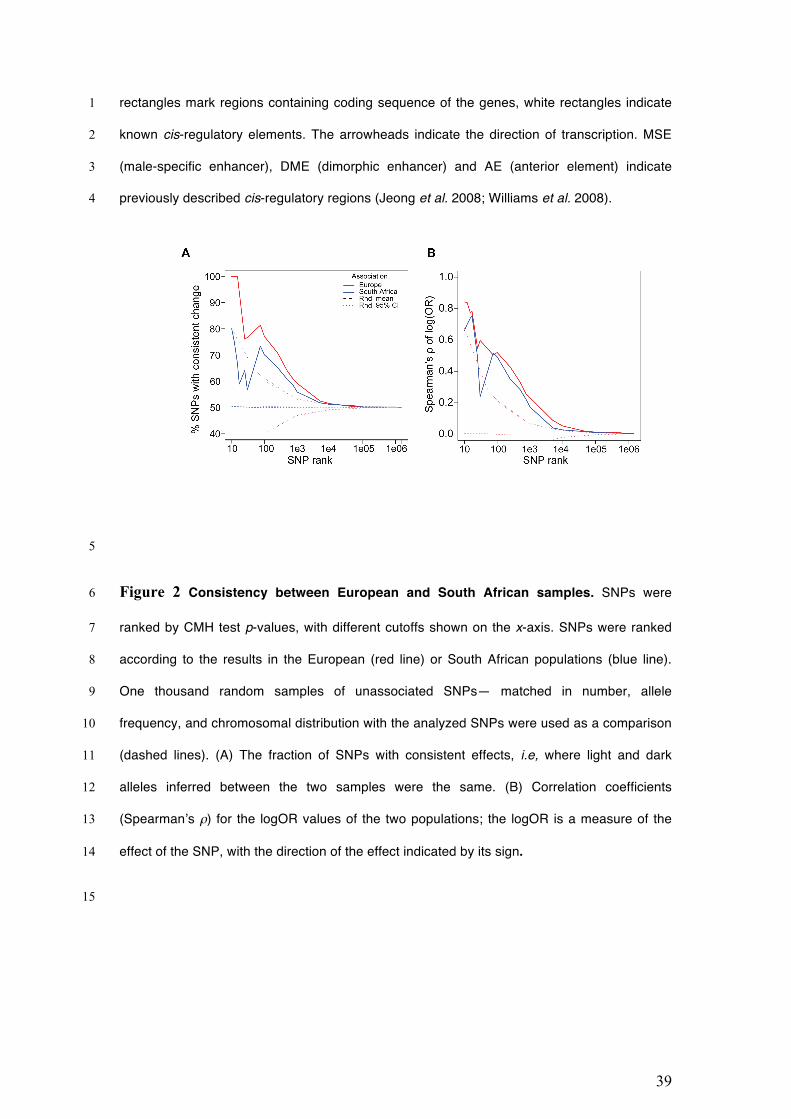
39

rectangles mark regions containing coding sequence of the genes, white rectangles indicate 1

known cis-regulatory elements. The arrowheads indicate the direction of transcription. MSE 2

(male-specific enhancer), DME (dimorphic enhancer) and AE (anterior element) indicate 3

previously described cis-regulatory regions (Jeong et al. 2008; Williams et al. 2008). 4

5

Figure 2 Consistency between European and South African samples. SNPs were 6

ranked by CMH test p-values, with different cutoffs shown on the x-axis. SNPs were ranked 7

according to the results in the European (red line) or South African populations (blue line). 8

One thousand random samples of unassociated SNPs— matched in number, allele 9

frequency, and chromosomal distribution with the analyzed SNPs were used as a comparison 10

(dashed lines). (A) The fraction of SNPs with consistent effects, i.e, where light and dark 11

alleles inferred between the two samples were the same. (B) Correlation coefficients 12

(Spearman’s ρ) for the logOR values of the two populations; the logOR is a measure of the 13

effect of the SNP, with the direction of the effect indicated by its sign. 14

15

40

1 2

Figure 3 Rejection Sampling Results. Heatmap showing the percentage of accepted 3

simulations using an ABC rejection method with 2,000,000 simulations uniformly sampling 4

parameter space and an acceptance rate of 1% using these criteria: 5

(logOR(tan)/logOR(bab1): Europe=2.51, South Africa=0.68; logOR(tanEU)/logOR(tanSA)=2.28 6

and logOR(bab1EU)/logOR(bab1SA)=0.62). Parameters were sampled uniformly from [-0.125, 7

1.125] for dominances and [0.25,4.5] for the additive effect of bab1 relative to tan. For 8

presentation in a grid, the parameter values were binned into intervals of 0.25 for dominance 9

and 1 for relative additive effect. The axes labels indicate the center of each binning interval. 10

The numbers in the cells give the percentage of accepted simulations in each binned 11

parameter interval. Each cell represents a particular range of combinations of dominance of 12

the light alleles at bab1 (top axis) and tan (bottom axis), and the relative additive effect of 13

bab1 to tan loci (left axis). 14

15

16

17

0.5

12

34

rela

tive

effe

ct b

ab1:

tan

bab1 locus

0 0.25 0.5

0.75 1 0 0.25 0.5

0.75 1 0 0.25 0.5

0.75 1 0 0.25 0.5

0.75 1 0 0.25 0.5

0.75 1

0 0.25 0.5 0.75 1

1.2 5.71.7

1.61.3

1912

3.3 7.66.81.4

8.1267.62.8

0 10 20 30Percent Accepted

9.1

dominance

tan locusdominance

41

1 2

3

Table 1. The four best candidate SNPs at the tan and bab loci. SNPs were selected based 4

on their rank in both studies, and had consistent allelic effects in both populations (i.e, the 5

identity of the putative light and dark alleles were consistent between Europe and South 6

Africa). The mean allele frequencies for these SNPs and their ratios of log odds ratios were 7

used in simulations and rejections sampling procedures, as described in the text. AF: allele 8

frequency of the ‘light’ allele, OR: odds ratio. P-values and odds ratios were obtained from the 9

CMH procedure. 10

11

EUROPE SOUTH AFRICA

CHR BPS AF -log10P logOR AF -log10P logOR logOR (EU)/

logOR (SA)

X 9120922 0.22 56.78 2.39 0.29 10.64 1.26

X 9121094 0.18 60.35 3.14 0.17 8.58 1.18

X 9121129 0.18 60.35 2.86 0.16 13.50 1.66

X 9121177 0.21 36.45 1.83 0.06 6.96 1.43

tan MEAN 0.20 2.55 0.17 1.38 1.89

3L 1084990 0.90 8.38 1.20 0.52 42.41 3.03

3L 1085137 0.85 4.35 0.65 0.47 37.04 2.54

3L 1085454 0.85 23.41 1.64 0.58 25.65 2.00

3L 1086356 0.73 4.54 0.57 0.30 23.81 2.06

bab MEAN 0.83 1.02 0.47 2.41 0.44

logOR (tan) / logOR

(bab) 2.51

0.57