reconciling micro and macro estimates of the frisch … · finance and economics discussion series...

Finance and Economics Discussion SeriesDivisions of Research & Statistics and Monetary Affairs

Federal Reserve Board, Washington, D.C.

Reconciling Micro and Macro Estimates of the Frisch LaborSupply Elasticity

William B. Peterman

2012-75

NOTE: Staff working papers in the Finance and Economics Discussion Series (FEDS) are preliminarymaterials circulated to stimulate discussion and critical comment. The analysis and conclusions set forthare those of the authors and do not indicate concurrence by other members of the research staff or theBoard of Governors. References in publications to the Finance and Economics Discussion Series (other thanacknowledgement) should be cleared with the author(s) to protect the tentative character of these papers.

Reconciling Micro and Macro Estimates of the Frisch Labor Supply

Elasticity

William B Peterman∗

Federal Reserve Board of Governors

October 15, 2012

Abstract

There are large differences between the microeconometeric estimates of the Frisch laborsupply elasticity (0-0.5) and the values used by macroeconomists to calibrate general equilibriummodels (2-4). The microeconometric estimates of the Frisch are typically estimated by regressingchanges in hours on changes in wages conditional on the individual being a married male head ofhousehold, working some minimum number of hours and being of prime working age. In contrastmacroeconomic calibration values are typically set such that fluctuations in a general equilibriummodel match the observed changes in the aggregate hours and wages from the whole populationover time. This paper aims to explain the gap by estimating an aggregate Frisch elasticitywhich is consistent with the concept of macro calibration values using the microeconometrictechniques. In order to estimate the Frisch consistent with the macro concept, this paper altersthe typical microeconometric approach in order to incorporate fluctuations on the extensivemargin and also broadens the scope of the sample to include single males, females, secondaryearners, young individuals, and old individuals. This paper finds that estimates of the aggregatemacro Frisch elasticity are in the middle of the range of macroeconomic calibration values(around 3.0). Furthermore, it finds that the key to explaining the difference are the fluctuationson the extensive margin of single males, females, secondary earners, older individuals, andyounger individuals.

JEL: E24, and J22.

Key Words: Frisch labor supply elasticity; intensive margin; extensive margin; calibration.

∗E-mail: [email protected]. Views expressed in this paper are my own and do not reflect the view ofthe Federal Reserve System or its staff. For extensive discussions and helpful comments, I thank Glenn Follette, LeahBrooks, Roger Gordon, Julie Cullen and Gordon Dahl, as well as seminar participants at the Federal Reserve Boardof Governors, 2012 System Applied Micro Conference, University of California at San Diego, and the Federal ReserveBoard of Governors. I am extremely grateful to Michael Barnett for excellent research assistance.

1

1 Introduction

The Frisch labor supply elasticity is a key economic variable for economists. It is central for

the design and assessments of government policies that affect labor supply and for analyzing the

macroeconomy. Despite the importance of the Frisch elasticity, there are large differences between

microeconometric estimates of this parameter and the values that are included in macroeconomic

models. The original microeconometric estimates of the Frisch elasticity are between 0 - 0.54 (see

MaCurdy (1981) and Altonji (1986)). These estimates are determined by regressing changes in

the natural log of an individual’s labor supply on wages over his life cycle accounting for possible

endogeneity of wages. In contrast, economists calibrate the Frisch elasticity in macroeconomic

models in the range of 2 - 4.1 These parameter values are calibrated by matching the volatility of

hours in a macroeconomic model and the aggregate volatility observed in the data over the business

cycle.

It is not surprising that there is a gap between these values since there are fundamental dif-

ferences in the concepts they are trying to capture. The microeconometric estimates evaluate the

Frisch elasticity conditional on the individual being employed, married, prime-aged, and the head

of the household. I refer to the Frisch elasticity consistent with this definition as the micro Frisch

elasticity. In contrast, the calibration values represent the aggregate Frisch elasticity considering

all the observed data. Specifically, these values incorporate aggregate changes in hours from all in-

dividuals and the observed aggregate changes in wages from workers. I refer to the Frisch elasticity

consistent with this definition as the macro Frisch elasticity. This paper determines whether the gap

between the microeconometric estimates and the calibration values used in macroeconomic models

can be explained by two key differences due to their alternate definitions.2 First, the original micro

econometric estimates are restricted to males who are married, primary earners, and between the

ages 26 to 60.3 In contrast, the aggregate volatility used for calibration includes observed fluctua-

tions from the whole population. Second, the microeconometric estimates include only fluctuations

1See Chetty et al. (2011) for a discussion of the values used to calibrate models.2Some alternative explanations include: utilizing weak instruments; disregarding the life cycle effect of endogenous-

age specific human capital; omitting correlated variables such as wage uncertainty; and not accounting for labormarket frictions such as liquidity constraints (see Imai and Keane (2004), Pistaferri (2003), Chetty (2009), Domeijand Floden (2006), and Contreras and Sinclair (2008)). Keane (2012) summarize the individual effect of some ofthese explanations on the estimates of the Frisch elasticity along with the effect of the extewnsive margin. Thesealternative explanations are not explored in this paper.

3Some of the original estimates are from an even narrower age range.

2

on the intensive margin, while the calibration values used in macroeconomic models incorporate

fluctuations in hours on both the intensive and extensive margin.

The goal of this paper is to determine whether estimates of the macro Frisch elasticity deter-

mined using the original microeconometric techniques in Altonji (1986) and MaCurdy (1981) are

consistent with values used to calibrate macroeconomic models. In order to estimate the macro

Frisch elasticity, I alter their estimation procedure in two ways. First, I broaden the composition

by including non-married individuals, females, secondary earners, younger individuals, and older

individuals.4 Second, I incorporate fluctuations in hours on the extensive margin and use a pseudo

panel instead of a traditional panel to estimate the macro Frisch. A pseudo panel is a panel data

set that constructs estimates of a cohort’s average over times from repeated cross sections. This

approach implies that instead of estimating the parameter values directly from changes in an indi-

vidual’s values over time, the estimates are determined from changes in the cohort’s average. This

approach offers a natural framework for estimating the macro Frisch elasticity since it estimates

the aggregate value for the representative cohort.5 Moreover, since the natural log of hours is

undefined if an individual works zero hours, but the cohorts average is still defined if non-workers

are included, using a pseudo panel allows me to incorporate individuals who do not work.

I estimate in a traditional micro panel that the micro Frisch elasticity which is conditional

on being a male, employed, married, a head of household, and between the ages of twenty-six to

sixty is approximately 0.2. In contrast, when I change the composition to be more inclusive and

incorporate fluctuations on the extensive margin, I estimate using a pseudo panel that the macro

Frisch elasticity is between 2.9 and 3.1. Therefore, the effect of these two differences arising from

alternative concepts of the Frisch elasticity can explain the gap between the microeconometric

estimates of the Frisch elasticity and the calibration values used in macroeconomic models. Next,

I individually determine the effect of adopting these changes on the micro estimates of the Frisch

elasticity. I find that when I include a broader composition, but only incorporate fluctuations on

the intensive margin, the estimates of the Frisch elasticity increase from 0.2 to 0.9. Alternatively, I

find that the estimates of the Frisch elasticity increases to between 0.8 and 0.9 when I incorporate

4When estimating the macro Frisch elasticity I focus on individuals between the ages of twenty and sixty-five.Ideally, I would include all individuals who were of working age, however because of data constraints I am forced tolimit the sample.

5Verbeek et al. (1992) demonstrates that if the size of the panel is large enough, coefficients estimated from apseudo panel will be unbiased estimates of the coefficients from a traditional panel.

3

fluctuations on the extensive margin but only examine males who are employed, head of their

household, of prime age, and married. Comparing the increases from incorporating each of these

changes independently indicates that both explanations play a similar role in reconciling the gap

between the microeconometric estimates and macro-calibration values. Furthermore, since the sum

of the changes from independently accounting for these differences is not large enough to explain

the gap, it is clear that the interaction of these two differences is important for explaining the

gap. Specifically, fluctuations on the extensive margin of single males, females, secondary earners,

older individuals, and younger individuals are critical to explaining the differences between the

microeconometric estimates of the Frisch elasticity and the values used to calibrate macroeconomic

models.

Although the goal of this paper is not to evaluate the original microeconometric approach to

estimating the Frisch elasticity, I test the sensitivity of the results with respect to the functional

forms of the instruments used to account for endogeneity bias to determine the robustness of the

results. I find that when I change the estimation procedure to use a more flexible set of polynomials

of the instruments, the difference between my estimates of the micro and macro estimates are still

large enough to explain the gap. Additionally, I estimate both the micro and macro Frish elasticity

for different age ranges in order to determine the importance of older individuals in both estimates.

When estimating the micro Frisch elasticity, I find that the estimates are fairly stable regardless of

the range of ages included in the estimating sample. With regards to the macro Frisch elasticity,

I find that excluding individuals between the ages of fifty-six to sixty-five causes the estimates

to drop by almost half. These results indicate that the fluctuations in aggregate hours of older

individuals are responsible for the large values calibrate the Macro Frisch elasticity are driven in

large part by .

This work builds on previous literature that examines whether either of these differences can

explain the gap. However, prior studies tend to examine each explanation in isolation and find

that neither can fully explain the gap on its own. Examples of previous work which demonstrates

that the sample’s composition can affect estimates of the Frisch elasticity include: Rıos-Rull et al.

(2012), Mulligan (1995), Heckman and Macurdy (1980), Blau and Kahn (2007), Fiorito and Zanella

(2012), and Kimmel and Kniesner (1998). These works tend to indicate that married men have

a lower Frisch elasticity than females, single males, and younger or older individuals.6 Although

6Some of these works focus on compensated elasticities as opposed to the Frisch elasticity. For example, Kimmel

4

these studies find that broadening the sample to include more than just married men who are the

head of their household increases the estimated Frisch elasticity, the authors do not incorporate

fluctuations on the extensive margin and therefore do not find that their estimates of the Frisch

elasticity are as large as the calibration values used in macroeconomic models.

Rogerson and Wallenius (2009) point out that because of different treatment of fluctuations on

the extensive margin “micro and macro elasticities need not be the same, and ... macro elasticities

can be significantly larger.”7 Using simulated data from a calibrated life cycle model they find that

including or excluding fluctuations on the extensive margin could cause large enough differences in

the estimates of the Frisch elasticity to explain the gap. In order to estimate the effect of the exten-

sive margin, Chetty et al. (2011) independently determine the parts of the macro Frisch elasticity

from the intensive and extensive margins using a meta analysis of separate quasi-experimental stud-

ies. They use the estimates of the participation rate elasticity to determine the portion of the macro

Frisch elasticity that comes from the extensive margin. These estimates, centered around 0.9, are

not as large as the difference between the microeconometric estimates and the macro-calibration

values. However, using the participation rate elasticity to incorporate fluctuations on the extensive

margin requires the strong assumption that the average hours worked are the same for new and

incumbent workers (see appendix A for more details). Instead of relying on this assumption, I use

a pseudo panel which allows me to estimate the whole macro Frisch elasticity directly from the

data, as opposed to separately estimating the parts of the macro Frisch elasticity.

Three exceptions in which the authors examine both differences in tandem are Mulligan (1999),

Faberman (2010), and Fiorito and Zanella (2012). The three studies estimate a Frisch elasticity

consistent with the micro definition in the range of 0.1 to 0.7. Additionally, the authors’ estimates

of the Frisch elasticity increase to a range of 0.6 to 1.4 when they include a larger composition and

incorporate fluctuations in hours on the extensive margin. In contrast to this paper, the difference

between these ranges are not large enough to explain the gap between the original microeconometric

estimates and the macro calibration values. The inability of these studies to show that the alternate

definition explain the gap is because they use alternate approaches to estimate the Frisch elasticity

and Kniesner (1998) demonstrates that married and single individuals have different compensated elasticities. Al-though Frisch elasticities and compensated elasticities can be different, the variation in the compensated elasticitybetween the various groups indicates that there will also tend to be variation in the Frisch labor supply elasticityfrom the various groups.

7Chang (2011) show that estimates of the micro elasticity from aggregate data that includes a decision on theextensive margin will include large biases.

5

in relation to this paper and the original microeconometric studies.

Similar to Altonji (1986) and MaCurdy (1981), I account account for the possible endogeneity of

wages by using age and education as an instrument. This approach implies that the Frisch elasticity

is identified off of predicted changes in wages over the lifetime. In contrast, Faberman (2010), and

Mulligan (1999) do not account for the possible bias when estimating the Frisch elasticity in a pseudo

panel. Since the authors do not instrument wages, they implicitly assume that the evolution of the

cohort’s average wage as the cohort ages is not correlated with unexpected changes in marginal

utility. If any of the unpredicted changes in wages is correlated with unexpected changes in marginal

utility, then the authors’ estimates will be biased, and this bias could possibly lead to the authors’

lower estimates of the macro Frisch elasticity.

Although, similar to this paper, Fiorito and Zanella (2012) accounts for the possible endogeneity

of wages, there are two differences in their estimation procedure. First, the authors just regress

the changes in aggregate hours on aggregate wages in a time series as opposed to a panel. This

approach ignores the panel dimension of the data and instead each observation in their data set

is the average of all individuals at a given point in time. Second, the authors use lagged wages

as instruments to account for the possible endogeneity bias. Their approach identifies the Frisch

elasticity from persistent changes in aggregate wages. One concern is that if individuals cannot

parse the transitory, persistent, and permanent part of shocks to wages, then lag wages will still be

correlated with unexpected changes to marginal utility. Moreover, not using the panel dimension

of the data could lead to a less efficient estimate.

I decompose the effects of ignoring the panel structure and using lagged wages as instruments. I

find that both of these alterations to the original microeconometric techniques cause lower estimates

of the macro Frisch elasticity, especially using the alternative wage. Therefore, if these alternative

instruments are more susceptible to being endogenous, then the studies using these as instruments to

determine the macro Frisch elasticity might underestimate the impact of the definitional differences.

Although the aim of this paper is not evaluate the various estimation strategies, it is important to

distinguish the implicit assumptions from these different estimation strategies since the differences

are the primary cause for this paper finding different results than Fiorito and Zanella (2012).

The rest of the paper is organized as follows: Section 2 derives the estimation equations from a

simple labor supply model. Section 3 describes the data and discusses how I construct the pseudo

6

panel. Section 4 presents the estimates of the micro and macro Frisch elasticity, while section 5

examines the robustness of the estimates. Section 6 concludes.

2 Labor Supply Model

In this section, I introduce the typical maximization problem for an individual. Next, I solve for

the first order conditions and manipulate them to create two different specifications that can be

used to estimate the Frisch elasticity in a reduced form setting. I demonstrate why estimates

based from these specifications may be susceptible to omitted variable bias. Finally, I introduce

the specific estimation strategies used in Altonji (1986) which are designed to account for these

omitted variables and describe why I focus on just one to estimate the Frisch.8

2.1 Individual’s Decisions

Employing a typical utility function that is homothetic and separable in consumption and labor,

an individual at age s solves the following problem,

maxEs

J∑j=s

βj−1

(χci,j

µ

1 + µc

1+ 1µ

i,j − χhi,jγ

1 + γh

1+ 1γ

i,j

)(1)

subject to

ci,j + ai,j+1 = wi,jhi,j + (1 + rt)ai,j , (2)

where Es represents the expectation operator at age s, J is the age of death, ci,j is consumption of

individual i at age j, h is hours worked, χci,j is a parameter that controls the taste for consumption,

χhi,j is a parameter that controls the taste for work, β is the discount rate, aj is savings, and rt is

the after tax return to savings. The first order conditions for the individual are

λj = χci,jc1µ

i,j (3)

λjwj = χhi,jh1γ

i,j (4)

8Since the estimation strategy in MaCurdy (1981) is replicated in Altonji (1986), the estimation strategies in Altonji(1986) serve as a complete set. Therefore, for notational convenience, I only cite Altonji (1986) when discussing theestimation strategies.

7

λj = EjβΨj,j+1(1 + r)λj+19 (5)

where λ is the marginal utility of consumption. The parameter of interest, γ, is the Frisch labor

supply elasticity. I derive two different specifications which have been used to determine γ. By

taking the logs and combining equations 3 and 4, I derive the first specification which relates hours

to consumption, tastes, and wages

lnhi,j = γ[1

µln ci,j + lnχci,j − lnχhi,j + lnwi,j ]. (6)

I derive the second specification by taking the difference between two ages of the log of equation 4,

∆ lnhi,j+1 = γ[∆ lnλi,j+1 + ∆ lnwi,j+1 − ∆ lnχhi,j+1] (7)

where ∆ represents the change over one year. Defining ξi,j+1 ≡ λi,j+1 − Eλi,j+1, the unexpected

changes to marginal utility, and combining equations 5 and 7 the second specification used to

determine γ can be written as

∆ lnhi,j+1 = γ[− lnβ − ln(1 + rt) + ξi,j+1 + ∆ lnwi,j+1 − ∆ lnχhi,j+1]. (8)

This second specification relates the change in hours to the change in wages and preference param-

eters. I refer to equation 6 as the level specification and equation 8 as the change specification.

The original estimates of the Frisch elasticity, such as those by Altonji (1986) and MaCurdy

(1981), came from estimating equations based on equations 6 and 8. When estimating the Frisch

elasticity with these equations, there is a general concern about omitted variables because taste

parameters and the unexpected changes to marginal utility can be correlated with wages. When

estimating these equations, it is important to either use instruments for wages or control for these

unobserved variables. There is an additional concern about measurement error. Most individu-

als are not paid hourly. Therefore, to determine an hourly wage, typically economists divide an

individual’s total income by the total hours he works in a given period. This procedure leads

to the possibility that the hours and wage estimates contain correlated measurement error. This

measurement error is an additional reason why instruments are typically used for wages.

9This is the intertemporal Euler equation for an individual at the age j. If the individual is solving at a differentage then the expectation operator should adjusted accordingly.

8

The original estimates of the Frisch elasticity were done using a specification based on equations

6 and 8. The estimation equations used are

lnhi,j = γ lnwi,j + β ln ci,j + ζTSi,j + ei,j (9)

∆ lnhi,j+1 = γ∆ lnwi,j+1 + δ + ζ∆TSi,j + εi,j , (10)

where hi,j is hours worked for the individual i at the age j, TS is a vector of variables controlling

for tastes, and δ is a set of annual dummies.10 Altonji (1986) estimates the Frisch elasticity with

three different versions of the two specifications. The first two estimates (table one and two in

Altonji (1986)) are based off of the change specification. His third estimate (table four in Altonji

(1986)) is based off of the level specification.

I implement the specification from table 2 of Altonji (1986) because the other estimation strate-

gies (table 1 and table 4) in Altonji (1986)) can only be estimated on a small subset of the entire

population.11 In this specification, the author uses age, education, education squared, interactions

between age and the polynomials of education, the education of the parents, and the parents’

economic status as instruments for wages.12 These instruments are used to account for both mea-

surement error and unexpected changes to marginal utility.13 Since these variables are known prior

to going into a period, one would not expect them to be correlated with unexpected shocks to

marginal utility. In other words, by using these instruments, the economist is identifying the re-

sponsiveness of hours to expected changes in wages over the life cycle. One concern is that age could

be correlated with changes in tastes. Therefore, I add some additional controls to the regression in

order to control for these possible changes.14

When estimating the macro Frisch elasticity, one complication is how to incorporate individuals

who work zero hours since the natural log of zero is undefined. I choose to estimate the Frisch

elasticity which incorporates individuals who do not work using a pseudo panel. Using a pseudo

10δ is included in the change specification to control for annual changes in the after tax return to capital.11In both alternative estimates the author uses a second wage series in the data that exists only for hourly employees.12The variable indicating economic status for the parents is not available for secondary workers. Therefore, I do

not present results using this instrument. However, in the sample that contained parental economic status, I foundthat excluding this instrument did not impact the results.

13I focus on the specifications in columns one and three that include age as an instrument but not as a control.14The variables I include to control for tastes are whether an individual lives in a city with a population larger

than 500,000, the number of children, and the number of children under six.

9

panel implies that I treat the cohort’s average at each age as an observation.15 A pseudo panel is

a natural setting in which to estimate the macro Frisch elasticity because it identifies the elasticity

from the aggregate response of the cohort’s average hours worked.

Using a pseudo panel does not come without disadvantages. Ideally, one would use the true

average of the whole cohort when creating the pseudo panel. However, I am limited to forming

the cohort’s averages from the sample that is observed in the data set.16 When using a pseudo

panel, the economist is implicitly treating the averages from the synthetic cohort as approximations

of the true cohort’s average. Treating a pseudo panel as a genuine panel can cause bias due to

measurement error introduced by not observing the true average. However, Verbeek et al. (1992)

demonstrates that with a sufficient number of individuals a pseudo panel can be treated as a genuine

panel without introducing an economically significant amount of bias.17

3 Data

Similar to Altonji (1986), I use the Michigan Panel Study of Income Dynamics (PSID). I utilize

the waves from 1968 until 1997.18 I use similar procedures to clean the data as employed in Altonji

(1986). The PSID only reports hourly wages for individuals who are paid on an hourly basis.

Therefore, I create a real hourly wage variable for everyone by taking the labor earnings divided by

the product of annual hours working for pay and consumption price index for urban individuals.

Following Altonji (1986), observations which exhibited a 250 percent increase or 60 percent decrease

in wages or consumption were treated as missing. Furthermore, observations with swings of more

than $13 or wages less than $0.40 in 1972 dollars were treated as missing.19 I do not observe the

wealth of the parents for secondary earners. Therefore, I exclude these variables as instruments

for changes in wages. I found that making these alterations did not affect the results on the group

15In order to estimate equation 8, I use the natural log of the average value of the cohort as opposed to the usingthe average natural log of the cohort’s value. Using the natural log of the average value corresponds to determiningthe parameter value that governs the representative cohort.

16This approach was originally proposed by Deaton (1985) to transform cross sectional data into panel data.17One difference from Verbeek et al. (1992) is that since my data set is a traditional panel, generally the cohort

contains the same individuals over time, while their data set is from repeated cross-sections. A consequence of theirdata is that there is more change in which individuals are observed. You would expect that a pseudo panel built froma traditional panel with a more consistent set of individuals to be less susceptible to this bias. However, the size ofthe data set employed in this study is on the lower end of the requirements discussed in Verbeek et al. (1992) so theestimates of the coefficients might be attenuated.

18After 1997 the PSID became bi-annual and therefore, I do not include these surveys.19Observations from non-working individuals are not subjected to this requirement.

10

of individuals for which I have complete coverage. Finally, I adjusted the age variable when an

individual reported no change in their age between the annual surveys or reported a change of

larger than one year.

Figure 1 plots the average annual hours by age for five different groups of people.20 These plots

are constructed by taking the traditional panel (pseudo panel) and averaging across all individuals

(cohorts) by age. The black line is the average annual hours for all individuals. Compared to the

other four lines, which are plots of the average hours for the subset of the sample that is working,

the profile for all individuals decreases much more rapidly towards the end of the working life. This

rapid decent indicates that many older aged individuals stop working. Figure 2 plots the average

wage profiles for various groups of individuals by age. The wage profiles tend to be upward sloping

over a majority of the lifetime for all the different groups. The black line plots the average of all

the observed wages which is used to estimate the macro Frisch elasticity.

Figure 1: Hours

1,800

2,000

2,200

2,400

nnua

l Hou

rs

1,200

1,400

1,600

,

20 25 30 35 40 45 50 55 60 65

Aver

age A

n

Working Married MalesWorking MalesWorking Head of HouseholdsAll Working IndvidualsAll Individuals

20 25 30 35 40 45 50 55 60 65Age

Figure 2: Wages

$0

$1

$2

$3

$4

$5

$6

$7

20 25 30 35 40 45 50 55 60 65

Aver

age

Hou

rly

Wag

e ($

1972

)

Age

Working Married Males

Working Males

Working Head of Households

All Working Indviduals

All Individuals (observed wages)

4 Estimates of Micro and Macro Frisch Elasticity

I start by replicating the estimates in Altonji (1986) from column I and III of his table 2. The

specification used to produce these estimates is a version of equation 10. Similar to Altonji (1986),

I estimate the Frisch elasticity by regressing the change in the natural log of hours on the change in

wages using age, education, education squared, interactions between education and age, mother’s

education, and father’s education as instruments for wages. These estimates are consistent with

20These plots are not the pseudo panels.

11

the definition of the micro Frisch elasticity.

Table 1 presents my benchmark estimates of the micro Frisch elasticity. Columns I-IV present

regression results when I do not include annual dummy variables, and columns V-VIII are the results

when I include annual dummies. Consistent with the definition of the micro Frisch elasticity, these

estimates are from a sample which only includes males who are the head of their household, are

married throughout the sample, are working throughout the whole sample, and are between the

ages of 26 and 60.21 Column I and IV presents the estimates when I restrict the sample to the same

period that is used in Altonji (1986) (1968-1981). The estimates (0.34 & 0.52) are close to those

originally presented in Altonji (1986) (0.28 & 0.48).22 I find that the F-statistic for the excluded

instruments in the first stage is 13.6 and 5.4 when I do not and do use annual dummies, respectively.

The lower value for the specification that includes annual dummies indicates that there is some

concern that the instruments are not relevant when annual dummies are included.23 The P-value

on the Hansen J-statistic for overidentification of the instruments is larger for the specification that

includes annual dummies which indicates that including annual dummies leaves less unexplained

variation in the second stage. The P-values are large enough in both specifications so as to not

raise concerns that the instruments are invalid.

Column II and VI of table 1 present estimates of the micro Frisch elasticity when I extend the

sample to include the years through 1997. Extending the data set to include more years causes the

two estimates of the Frisch elasticity to converge to approximately 0.20. I proceed by using all these

years of the PSID in the rest of the regressions. One concern about the original estimation strategy

is that there may be an omitted variable bias because age could be correlated with changes in tastes.

Therefore, I include indicator variables for whether the individual lives in a big city, the number

of children in the household, and the number of kids under the age of six in the household, each of

which should be correlated with omitted changes in tastes. The estimates that include these controls

for changes in tastes are in columns III and VII. I find that controlling for tastes causes the point

21Individuals who are not actively working, students, retired or work less than 250 hours a year, are considered tonot be working and excluded from his data set. Formally, I consider individuals to not be working in a specific yearif they report working less than or equal to 250 hours. As opposed to considering any individual who works less than250 hours non-working, Altonji (1986) uses a cutoff of zero hours. I choose to use a higher threshold because I amnot able to utilize all of the variables that contain reported information about retirement since the variables do notexist for secondary earners.

22There are a few reason for slight differences in the estimates. First, I use the weights in the PSID. Second, I wasunable to replicate his restrictions for undetermined reasons. Third, I use the Consumer Price Index to deflate wagesas opposed to the GDP deflator.

23The F-statistic is lower when annual dummies are included because there are less degrees of freedom.

12

estimates of the Frisch to increase slightly. Although the changes are not statistically significant,

the increase indicates that omitting changes in tastes could cause a downward bias. Therefore, I

include these controls for changes in tastes in all subsequent regressions. Finally, columns IV and

VIII are estimates when I no longer require the panel to be balanced. Specifically, if individuals stop

working prior to age 60, their observations when they are working are still included. By allowing

the panel to be unbalanced, I increase the number of observations by over ten percent; however, the

estimates are nearly identical. Since this change does not alter the point estimates, but increases

the number of observations, I relax this restriction in all subsequent regressions. I treat columns

IV and VIII as my benchmark results for the micro Frisch elasticity which I use for comparison in

order to determine the effect of broadening the scope of the sample and including fluctuations on

the extensive margin.

One concern about these estimates is that the Hansen J-stat for overidentification of the in-

struments is low for all of the specifications that use the larger time period. The low J-stat is

a persistent problem in all my analysis. Despite concerns about validity, I continue because the

goal of this paper is to determine whether estimates of the macro Frisch using the microeconomet-

ric techniques are consistent with the values used to calibrate macroeconomic models. However,

because of this concern about validity, the point estimates should be interpreted with caution.

Next, I estimate the macro Frisch elasticity. These estimates use a pseudo panel which includes

the hours fluctuations from the extensive margin. Additionally, I broaden the scope of the sample

to include all individuals between the ages of twenty and sixty-five (the additional groups included

are females, secondary earners, younger individuals, older individuals, and single individuals). The

estimates of the macro Frisch elasticities are presented in table 2. The estimates range from 2.88

to 3.1 depending on whether annual dummies are included. I find that these estimates of the

macro Frisch elasticity are statistically different from the benchmark estimates of the micro Frisch

elasticity. Furthermore, the estimates of the macro Frisch elasticity are in the middle of the range

of the values used to calibrate macroeconomic models. Therefore, these results indicate that the

different treatment of fluctuations on the extensive margin and the different levels of inclusion of

individuals in the sample implied by the different definitions can reconcile the gap between the

microeconometric estimates and the macro-calibration values of the Frisch elasticity. Additionally,

when estimating the macro Frisch elasticity, the first stage passes the Hansen J-test indicating that

13

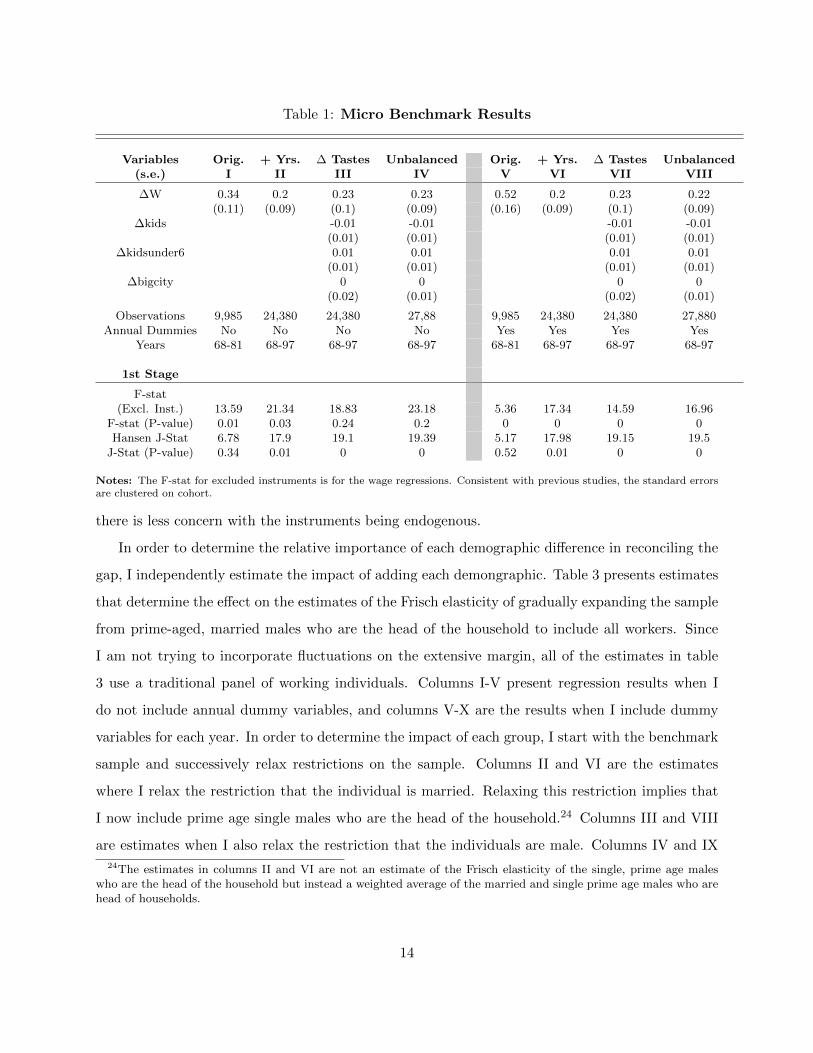
Table 1: Micro Benchmark Results

Variables Orig. + Yrs. ∆ Tastes Unbalanced Orig. + Yrs. ∆ Tastes Unbalanced(s.e.) I II III IV V VI VII VIII

∆W 0.34 0.2 0.23 0.23 0.52 0.2 0.23 0.22(0.11) (0.09) (0.1) (0.09) (0.16) (0.09) (0.1) (0.09)

∆kids -0.01 -0.01 -0.01 -0.01(0.01) (0.01) (0.01) (0.01)

∆kidsunder6 0.01 0.01 0.01 0.01(0.01) (0.01) (0.01) (0.01)

∆bigcity 0 0 0 0(0.02) (0.01) (0.02) (0.01)

Observations 9,985 24,380 24,380 27,88 9,985 24,380 24,380 27,880Annual Dummies No No No No Yes Yes Yes Yes

Years 68-81 68-97 68-97 68-97 68-81 68-97 68-97 68-97

1st Stage

F-stat(Excl. Inst.) 13.59 21.34 18.83 23.18 5.36 17.34 14.59 16.96

F-stat (P-value) 0.01 0.03 0.24 0.2 0 0 0 0Hansen J-Stat 6.78 17.9 19.1 19.39 5.17 17.98 19.15 19.5

J-Stat (P-value) 0.34 0.01 0 0 0.52 0.01 0 0

Notes: The F-stat for excluded instruments is for the wage regressions. Consistent with previous studies, the standard errorsare clustered on cohort.

there is less concern with the instruments being endogenous.

In order to determine the relative importance of each demographic difference in reconciling the

gap, I independently estimate the impact of adding each demongraphic. Table 3 presents estimates

that determine the effect on the estimates of the Frisch elasticity of gradually expanding the sample

from prime-aged, married males who are the head of the household to include all workers. Since

I am not trying to incorporate fluctuations on the extensive margin, all of the estimates in table

3 use a traditional panel of working individuals. Columns I-V present regression results when I

do not include annual dummy variables, and columns V-X are the results when I include dummy

variables for each year. In order to determine the impact of each group, I start with the benchmark

sample and successively relax restrictions on the sample. Columns II and VI are the estimates

where I relax the restriction that the individual is married. Relaxing this restriction implies that

I now include prime age single males who are the head of the household.24 Columns III and VIII

are estimates when I also relax the restriction that the individuals are male. Columns IV and IX

24The estimates in columns II and VI are not an estimate of the Frisch elasticity of the single, prime age maleswho are the head of the household but instead a weighted average of the married and single prime age males who arehead of households.

14

Table 2: Aggregate “Macro” Estimates

Variables Micro Macro Micro Macro(s.e.) I II III IV

∆W 0.23 3.1 0.22 2.88(0.09) (0.68) (0.09) (0.67)

∆kids -0.01 -0.28 -0.01 -0.28(0.01) (0.11) (0.01) (0.11)

∆kidsunder6 0.01 -0.21 0.01 -0.15(0.01) (0.14) (0.01) (0.12)

∆bigcity 0 1.09 0 0.18(0.01) (0.51) (0.01) (0.31)

Observations 27,880 1,288 27,880 1,288Yr. Dummies No No Yes Yes

Years 68-97 68-97 68-97 68-97Ages 26-60 20-65 26-60 20-65

1st Stage

F-stat(Excl. Inst.) 23.18 3.6 16.96 3

F-stat (P-value) 0.2 0.01 0 0Hansen J-Stat 19.39 6.38 19.5 10.81

J-Stat (P-value) 0 0.38 0 0.09


are the estimates when I also relax the restriction that individuals are the head of the household.

Finally, columns V and X are the estimates when I relax all the restrictions and also extend the

age range so that all working individuals between 20 and 65 are included.

I find that relaxing the marriage restriction causes an increase in the Frisch elasticity; however,

since the increase is not statistically significant it is only suggestive that single males may have a

higher Frisch. When I include females in columns III and VIII, the point estimates of the Frisch

elasticity decrease, but a statistically insignificant amount. The sign of the change is not surprising

since the group that is being added, females who are the head of the household, are likely less

responsive to temporary changes in their wages. I find that when I include secondary earners in my

sample the Frisch elasticity approximately doubles (columns IV and IX). I find that these estimates

which include secondary earners in the data are statistically different from both the benchmark

estimates (columns I and VI) and the prior estimates which exclude secondary earners in the data

set (columns III and VIII). Finally, when I include younger and older individuals in the sample the

estimates double again, a statistically significant increase. Comparing columns V and X to their

15

respective benchmarks (columns I and V), indicates that relaxing all these restrictions causes the

Frisch elasticity to increase by approximately 0.7, also a statistically significant increase.

Table 3: Composition Effects

Variables Micro +Single +Female +2nd Earn +Age Micro +Single +Female +2nd Earn +Age(s.e.) I II III IV V VI VII VIII IX X

∆W 0.23 0.35 0.29 0.55 0.93 0.22 0.32 0.26 0.55 0.91(0.09) (0.08) (0.08) (0.15) (0.11) (0.09) (0.08) (0.09) (0.14) (0.1)

∆kids -0.01 0 -0.01 -0.02 -0.02 -0.01 0 -0.01 -0.01 -0.02(0.01) (0) (0) (0) (0) (0.01) (0) (0) (0) (0)

∆kidsunder6 0.01 0.01 0.01 -0.03 -0.03 0.01 0.01 0 -0.03 -0.04(0.01) (0) (0.01) (0.01) (0.01) (0.01) (0) (0.01) (0.01) (0.01)

∆bigcity 0 0.02 0.02 0.02 0.02 0 0.02 0.01 0.02 0.02(0.01) (0.01) (0.01) (0.01) (0.01) (0.01) (0.01) (0.01) (0.01) (0.01)

Observations 27,880 49,178 64,259 87,910 104,348 27,880 49,178 64,259 87,910 104,348Yr. Dummies No No No No No Yes Yes Yes Yes Yes

Years 68-97 68-97 68-97 68-97 68-97 68-97 68-97 68-97 68-97 68-97

Restrictions

Married Yes YesMale Yes Yes Yes Yes

Primary Earner Yes Yes Yes Yes Yes YesAge 25 - 60 Yes Yes Yes Yes Yes Yes Yes YesAge 20 - 65 Yes Yes

1st Stage

F-stat(Excl. Inst.) 23.18 23.86 23.11 21.22 34.07 16.96 23.92 27.89 25.11 36.41

F-stat (P-value) 0.2 0 0 0 0 0 0 0 0 0Hansen J-Stat 19.39 16.36 23.73 30.57 23.87 19.5 18.55 25.79 30.34 23.53

J-Stat (P-value) 0 0.01 0 0 0 0 0 0 0 0


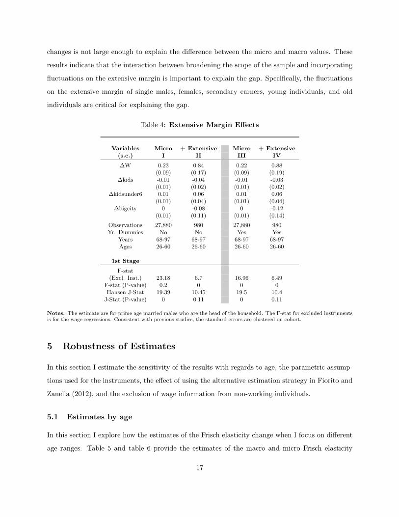
Table 4 tests the impact on the estimates of the Frisch elasticity of including fluctuations on

the extensive margin in the more restricted subset of the data that only include married males

who are the head of their household. In order to estimate the Frisch elasticity which includes

fluctuation on the extensive margin I use a pseudo panel.25 Since I am focusing on the impact of

the fluctuations on the extensive margin, I still limit my sample to married males who are the head

of their household. I find that the estimates of the Frisch elasticity increases to a similar level,

between 0.84 and 0.88, when I include fluctuations on the extensive margin as they did when I

broadened the sample. These increases are statistically significant.

Individually estimating the impact of both differences arising from the alternative definition,

I find that broadening the scope of the sample increases the estimates of the Frisch elasticity by

approximately 0.7. Moreover, I find that including fluctuations on the extensive margin increases

the Frisch elasticity by between 0.61 and 0.66. The increase from individually accounting for

each of these differences indicates that both explanations play an important role in reconciling

the gap between the microeconometric estimates and macro-calibration values. The sum of these

25These estimates of the impact of the extensive margin are consistent with the macro Frisch elasticity in the sensethat they do not account for the fluctuations in potential wages of non-working individuals.

16

changes is not large enough to explain the difference between the micro and macro values. These

results indicate that the interaction between broadening the scope of the sample and incorporating

fluctuations on the extensive margin is important to explain the gap. Specifically, the fluctuations

on the extensive margin of single males, females, secondary earners, young individuals, and old

individuals are critical for explaining the gap.

Table 4: Extensive Margin Effects

Variables Micro + Extensive Micro + Extensive(s.e.) I II III IV

∆W 0.23 0.84 0.22 0.88(0.09) (0.17) (0.09) (0.19)

∆kids -0.01 -0.04 -0.01 -0.03(0.01) (0.02) (0.01) (0.02)

∆kidsunder6 0.01 0.06 0.01 0.06(0.01) (0.04) (0.01) (0.04)

∆bigcity 0 -0.08 0 -0.12(0.01) (0.11) (0.01) (0.14)

Observations 27,880 980 27,880 980Yr. Dummies No No Yes Yes

Years 68-97 68-97 68-97 68-97Ages 26-60 26-60 26-60 26-60

1st Stage

F-stat(Excl. Inst.) 23.18 6.7 16.96 6.49

F-stat (P-value) 0.2 0 0 0Hansen J-Stat 19.39 10.45 19.5 10.4

J-Stat (P-value) 0 0.11 0 0.11

Notes: The estimate are for prime age married males who are the head of the household. The F-stat for excluded instrumentsis for the wage regressions. Consistent with previous studies, the standard errors are clustered on cohort.

5 Robustness of Estimates

In this section I estimate the sensitivity of the results with regards to age, the parametric assump-

tions used for the instruments, the effect of using the alternative estimation strategy in Fiorito and

Zanella (2012), and the exclusion of wage information from non-working individuals.

5.1 Estimates by age

In this section I explore how the estimates of the Frisch elasticity change when I focus on different

age ranges. Table 5 and table 6 provide the estimates of the macro and micro Frisch elasticity

17

for different age ranges, respectively.26 When I exclude individuals that are between sixty-one and

sixty-five, the estimate of the macro Frisch drops from 2.88 to 1.8. The estimate drops further to

0.8 when I exclude individuals between fifty-one and sixty-five. These significant drops indicate

that the macro Frisch elasticities are not consistent over all ages and that the large estimates are

primarily driven by older individuals. Examining the black lines in the plots of the average wage

and hours profiles in figures 1 and 2, it is clear that the average hours start dropping rapidly at

the age of fifty. However, during the same age range the cohort’s average wages stay fairly steady,

dropping only a small amount. Conversely, for younger individuals, the changes in the hours profile

are relatively small compared to the change in the wage profile. Therefore, if older individuals are

included, a large Frisch elasticity is needed to explain the relatively larger movements in the hours

profile than the wage profile. However, if older individuals are excluded, the estimates of the Frisch

elasticity are much smaller since the size of the relative movements in hours to wages is smaller.

One interpretation of these results is that the macro Frisch elasticity changes over the life cycle.

However, current research points to a possible alternate explanation. The original microeconometric

estimation strategy assumes that any predicted changes in the wages are due to market forces and

exogenous to the decision with regards to how many hours to work. Additionally, the estimation

strategy implicitly assumes that the causal relationship is such that any changes in hours are a

result of the changes in wages. However, some recent research has documented that these changes

in wages may not be exogenous from the hours decisions. Casanova (2012) examines whether

hours and wage dynamics for older people can be explained by partial retirement. The author

demonstrates that when one controls for partial retirement, the wage profile for older individuals

no longer falls but is upward sloping throughout the whole working lifetime. Further, she argues

that the transition out of full time work to either partial or full retirement is a choice for most

workers and the subsequent drop in the wage is endogenously determined. Specifically, the author

states that “while standard labor supply models would rationalize the reduction in hours worked

upon partial retirement as a response to an exogenously declining wage trajectory, the evidence

presented in the paper indicates instead that workers choose to trade more leisure for a lower hourly

wage in a context in which a better paid, full-time job is available.” In other words, individuals

preferences for leisure increase as they age causing them to choose to work less hours (partially

26I do not display the estimates when the annual dummies are not included; however, the results are similar.

18

retire) and receive a lower hourly wage.

The results in table 5, coupled with the finding in Casanova (2012), indicate that incorporating

older individuals in estimates of the macro Frisch elasticity, which includes fluctuations on the

extensive margin, may cause an upward bias. Specifically, if the changes in older individuals hours

are not a result of decreases in potential wages but instead older agents are jointly choosing lower

wages and hours in response to a increase in the desire for leisure, then a correctly specified estimate

of the Frisch elasticity would be lower. Since younger individuals are less likely to be affected by

partial retirement, it is likely that the estimates of the macro Frisch which only include these

younger individuals are less susceptible to bias from partial retirement. Therefore, individuals may

not be as responsive to changes in their wages as the macro Frisch elasticity estimates imply, but

instead this may be an artifact of not totally controlling for changes in preferences.

Overall, determining which value to use in a calibrated model depends crucially on which

question the economist is examining and how the model is specified. For example, if the model

being calibrated includes both a partial retirement decision and assumes the preferences for leisure

increase with age, then a lower value in line with the value estimated when only inlcuding younger

individuals should be used. Alternatively, if the model being calibrated is more parsimonious and

does not include either partial retirement or changes in preferences for leisure over the life cycle,

then in order for the model to replicate the observed wage and hours profiles, it will need to

include a larger macro Frisch value in line with the estimates which incorporate older individuals.

Furthermore, if the decision of when to retire is not relevant to the question being examined then

the relevant value for calibration is the estimate of the Frisch elasticity for younger individuals,

as opposed to the larger value estimated for all individuals. Conversely, if the total aggregate

fluctuations in labor including retirement are relevant to the question being examined, then the

larger Frisch elasticity estimated for the bigger age range is the more relevant estimate.

Table 6 presents the results when I estimate the micro Frisch for different ages. Unlike the esti-

mates of the macro Frisch, the decrease in the estimates are small when I exclude older individuals.

One explanation for the smaller changes is that the micro Frisch is estimated only on individuals

who are working and focuses on younger individuals who are less likely to be partially retired.27

Therefore, one needs to be less concerned about changes in the values over the life cycle when

27Since individuals are required to work a minimum number of hours in order to be included in the sample usedto estimate the micro Frisch, many individuals who are partially retired may be excluded.

19

Table 5: Macro Estimate by Age

Age RageVariables 20-65 20-60 20-55 20-50 20-45

(s.e.) I II III IV V

∆W 2.88 1.75 1.5 0.81 0.51(0.67) (0.35) (0.360) (0.25) (0.17)

∆kids -0.28 -0.11 -0.1 -0.03 -0.04(0.11) (0.05) (0.05) (0.03) (0.03)

∆kidsunder6 -0.15 -0.04 -0.01 0.09 0.16(0.12) (0.08) (0.07) (0.05) (0.05)

∆bigcity 0.18 0.15 0.17 0.17 0.08(0.31) (0.27) (0.25) (0.2) (0.19)

Observations 1,288 1,148 1,008 868 728Yr. Dummies Yes Yes Yes Yes Yes

Years 68-97 68-97 68-97 68-97 68-97

1st Stage

F-stat(Excl. Inst.) 3 4.85 8.39 3 6.17

F-stat (P-value) 0 0 0 0 0Hansen J-Stat 10.81 20.21 9.09 10.81 18.73

J-Stat (P-value) 0.09 0 0.17 0.09 0

Notes: The estimates are from a pseudo panel which includes all individuals. The F-stat for excluded instruments is for thewage regressions. Consistent with previous studies, the standard errors are clustered on cohort.

choosing calibration values for the Frisch elasticity only on the intensive margin.

5.2 Alternative Parametric Assumptions

The previous results demonstrate that the estimates of the macro Frisch elasticity decrease when

older generations are excluded. Additionally, since the large macro Frisch is particularly driven by

the fluctuations in wages predicted by the polynomials of the instruments from older individuals,

it is important to see if using predicted wages from a more flexible set of polynomials affects the

estimates of the macro Frisch. Therefore, in this section I explore the sensitivity of the results when

I use a more flexible set of polynomials of age and education as instruments. Specifically, I use up

to a third order Chebychev polynomial of age, second order Chebychev polynomial of education,

and the interaction of all the polynomials. Chebychev polynomials are a sequence of orthogonal

recursive polynomials. Using these orthogonal polynomials as instruments, as opposed to using

the quadratic polynomials, allows for more flexibility in the relationship between wages and the

instruments. Table 7 presents the results when I use these alternative polynomials.

20

Table 6: Micro Estimate by Age

Age RageVariables 25-60 25-55 25-50 25-45

(s.e.) I II III IV

∆W 0.22 0.17 0.07 0.05(0.09) (0.11) (0.12) (0.12)

∆kids -0.01 0 0 0(0.01) (0.01) (0.01) (0.01)

∆kidsunder6 0.01 0.01 0 0(0.01) (0.01) (0.01) (0.01)

∆bigcity 0 -0.01 -0.01 -0.01(0.01) (0.01) (0.01) (0.02)

Observations 27,880 25,459 21,939 17,774Yr. Dummies Yes Yes Yes Yes

Years 68-97 68-97 68-97 68-97

1st Stage

F-stat(Excl. Inst.) 16.96 16.96 10.65 9.07

F-stat (P-value) 0 0 0 0Hansen J-Stat 19.5 19.5 18.48 12.45

J-Stat (P-value) 0 0 0.01 0.05

Notes: The estimates are from a traditional panel which includes only prime age married males who are the head of thehousehold. The F-stat for excluded instruments is for the wage regressions. Consistent with previous studies, the standarderrors are clustered on cohort.

21

Table 7: Affect of Alternative Parametric Form

Variables Micro Bench. Micro Alt. Macro Bench. Macro Alt.(s.e.) I II III IV

∆W 0.22 0.2 2.88 2.28(0.09) (0.1) (0.67) (0.48)

∆kids -0.01 -0.01 -0.28 -0.19(0.01) (0.01) (0.11) (0.09)

∆kidsunder6 0.01 0 -0.15 -0.12(0.01) (0.01) (0.12) (0.11)

∆bigcity 0 0 0.18 0.83(0.01) (0.01) (0.31) (0.38)

Observations 27,880 27,880 1,288 1,288Yr. Dummies Yes Yes Yes Yes

Years 68-97 68-97 68-97 68-97Ages 26-60 26-60 20-65 20-65

Instruments Quadratics Chevycheb Quadratics Chevycheb1st Stage

F-stat(Excl. Inst.) 16.96 11.83 16.96 5.2

F-stat (P-value) 0 0 0 0Hansen J-Stat 19.5 21.5 19.5 17.17

J-Stat (P-value) 0 0.04 0 0.1


The first and third columns of table 7 are the benchmark estimates of the micro and macro

Frisch elasticity using the quadratic polynomials of the instruments, respectively. The second and

fourth columns are the estimates of the micro and macro Frisch elasticity using the Chebyshev

polynomials of the instruments, respectively. Comparing column I and II, it is clear that the

estimates of the micro Frisch elasticity are not sensitive to the different polynomials. Although the

estimate of the macro Frisch elasticity is somewhat smaller when I use the more flexible polynomials,

the decrease is not statistically significant. Furthermore, the estimate of the macro Frisch elasticity

with the alternative polynomials is still large enough to explain the gap between the original

microeconometric estimates of the Frisch and the values used to calibrate macroeconomic models.

Therefore, these results further indicate that the different treatment of fluctuations on the extensive

margin and the different composition of the samples can can explain the gap.

22

5.3 Comparison with Fiorito and Zanella (2012) Estimation Strategy

Similar to this exercise, Fiorito and Zanella (2012) also tries to determine if these differences in

definition could explain the large gap between microeconometric estimates of the Frisch and cali-

bration values used in macroeconomic models. Despite estimating a similar micro Frisch elasticity,

the authors estimate a macro Frisch elasticity that is much smaller than this study (0.6).

The authors use a different estimation strategy than the strategy used in this paper. As pre-

viously mentioned, when estimating the macro Frisch, this paper tries to use a strategy that is

close the Altonji (1986). Specifically, it estimates the macro Frisch in a pseudo pane using age

and education as instruments for wage. In contrast, Fiorito and Zanella (2012) use an alternative

approach in which they just use the change in the whole population’s averages over time as opposed

to the changes in the different cohort’s averages over time and use lagged wages as instruments

for current wages. Furthermore, the authors do not address the possible bias from not observing

changes in tastes for working.

Identifying the Frisch elasticity using lagged wages as instruments in a time series, as opposed

to age and education in a pseudo panel, implies that the estimates in Fiorito and Zanella (2012) are

being identified off of different types of fluctuations in wages. In particular, in this study the Frisch

is identified off of changes in a cohort’s wages over their life cycle that can be predicted by age and

education. In contrast, Fiorito and Zanella (2012) uses the variation in average wage across the

whole economy that can be predicted from changes in the previous periods. Therefore, this paper

identifies the Frisch elasticity by focusing on the life cycle changes in wages while Fiorito and Zanella

(2012) identifies the Frisch elasticity by focusing on the persistent portion of shocks to aggregate

wages. One concern is that if there is some uncertainty about how much of a shock to aggregate

wages is persistent versus transitory, then lag wages could still be an endogenous instrument because

they will be correlated with unexpected shocks to marginal utility. Furthermore, by not exploiting

the panel structure nor distinguishing cohorts, the procedure in Fiorito and Zanella (2012) will

produce estimates that are weakly less efficient and may be affected by changes in composition.

Table 8 explores the effect of these differences in the estimation strategy. The first column of the

table reproduces the benchmark estimates of the macro Frisch in a pseudo panel using the adapted

microeconometric strategy described in this paper. The second column provides estimates of the

macro Frisch using the same pseudo panel but switching to lagged wages as the instrument for

23

current wages as opposed to using age and education.28 I find that the estimates drop significantly

when I use these alternative wages in a pseudo panel to estimate the Frisch elasticity. The large

differences in the estimates indicate that lag wages could still be endogenous with current wages.

Furthermore, when I estimate the Frisch elasticity using lagged wages in a time series, as opposed

to a pseudo panel, the estimates (column III) fall even more.29 These results indicate that by

using this alternative strategy to estimate the Frisch elasticity, Fiorito and Zanella (2012) may

have underestimated the macro Frisch and consequently understated the ability of fluctuations on

the extensive margin and the different compositions to explain the gap between the macro and

micro Frisch elasticity.

Table 8: Affect of Specification in Fiorito and Zanella (2012)

Variables Benchmark Alt. Inst. No Panel & Alt. Inst.(s.e.) I II III

∆W 2.88 0.64 0.42(0.67) (0.23) (0.26)

∆kids -0.28(0.11)

∆kidsunder6 -0.15(0.12)

∆bigcity 0.18(0.31)

Observations 1,288 1,008 18Yr. Dummies Yes Yes No

Years 68-97 68-97 68-91Ages 20-65 20-65 20-65

Instruments Age & Educ Lag Wage Lag WageType of Data Pseudo Panel Pseudo Panel Time Series

1st Stage

F-stat(Excl. Inst.) 3 23.31 1.5

F-stat (P-value) 0 0 0.15Hansen J-Stat 10.81 6.38 4.5

J-Stat (P-value) 0.09 0.09 0.21


28Similar to in my benchmark macro estimates, the first stage regression is run on the cohort level as opposed tothe individual level.

29I choose to not use annual dummies due to a lack of degrees of freedom. Furthermore, I limit the sample periodwhen running the time series regression because Fiorito and Zanella (2012) point out that the wage variable mayhave fundamentally changed after 1992.

24

5.4 Unconditional Frisch Elasticity

This paper focuses on estimates of the aggregate Frisch elasticity consistent with the macro defin-

tion. These estimates are consistent with the calibration values used in macroeconomic models.

The macro Frisch elasticity is estimated from a pseudo panel which includes unconditional changes

in hours and the observed changes in wage which exclude the potential wages for non-working

(no-work) individuals.30 However, the estimates of the macro Frisch elasticity (table 2) are not

estimates of the unconditional aggregate Frisch elasticity because they do not include fluctuations

in potential wages from non-working individuals. Since it might be of interest, I also estimate the

unconditional value which accounts for possible selection bias from non-working individuals. In

order to account for selection bias, I follow the procedure in Fiorito and Zanella (2012) in which

the authors predict the wages for non-working individuals using a Heckman-type correction for se-

lection bias.31 Selected results from these regressions are in appendix B. Fiorito and Zanella (2012)

note that Blundell et al. (2003) shows empirically that when they create an aggregate wage which

includes a similar selection corrected predicted wage for non-workers, most of the aggregation bias

is removed from their aggregate wage series.

Table 9 presents the estimates of the unconditional aggregate Frisch elasticity. In order to

account for this possible selection bias when estimating the unconditional aggregate Frisch elasticity,

I use a Heckman-style correction and predict wages for non-working individuals similar to Fiorito

and Zanella (2012). One complication is that some individuals who indicate they retired or work

less than 250 hours still report labor income. Therefore, I estimate the Frisch elasticity with two

different wage series for each cohort. First, I incorporate predicted wages for individuals who do

not report any income and observed wages for others in the cohort’s average (predict missing).

Second, I incorporate predicted wages for individuals who report that they are retired or work less

than 250 hours and use the observed wages for others in the cohort’s average (predict non-working).

The estimates of the unconditional aggregate Frisch elasticity range from 1.68 to 2.64. I find that

when I control for selection bias by predicting wages for those who do not report wage information,

30In this estimate of aggregate wage, if an individual reports not working but still reports a wage that informationis included in the pseudo panel.

31See section 3 of Fiorito and Zanella (2012) and Wooldridge (1995) for more details on the correction procedure.The variables used to predict employment at the first stage are gender, race, marital status, number of kids and aset of polynomials and interactions between age and education. One difference between Fiorito and Zanella (2012)and this study is that the level, as opposed to the natural log, of wages is predicted.

25

the estimates of the Frisch elasticity are significant compared to the estimates of the macro Frisch

elasticity. However, when I only control for selection by predicting wages for all of those who

report not working the change in the estimates is statistically significant. These results indicate

that incorporating the wage information reported for individuals who also report not working causes

the estimate of the Frisch elasticity to be much lower.

Table 9: Aggregate Unconditional Frisch

Variables Macro Unconditional Unconditional Macro Unconditional Unconditional(s.e.) I II III IV V VI

∆ W(observed) 3.1 2.88(0.68) (0.67)

∆ W (predict missing) 1.68 1.78(0.45) (0.43)

∆ W (predict no-work) 2.41 2.64(0.36) (0.44)

∆kids -0.28 -0.16 -0.23 -0.28 -0.16 -0.21(0.11) (0.07) (0.06) (0.11) (0.06) (0.07)

∆kidsunder6 -0.21 -0.02 -0.15 -0.15 -0.06 -0.23(0.14) (0.08) (0.07) (0.12) (0.08) (0.08)

∆bigcity 1.09 0.18 0.12 0.18 0.63 0.41(0.51) (0.17) (0.18) (0.31) (0.27) (0.29)

Observations 1,288 1,288 1,288 1,288 1,288 1,288Yr. Dummies No No No Yes Yes Yes

Years 68-97 68-97 68-97 68-97 68-97 68-97Ages 20-65 20-65 20-65 20-65 20-65 20-65

1st Stage

F-stat(Excl. Inst.) 3.6 4.85 8.39 3 6.17 8.22

F-stat (P-value) 0.01 0 0 0 0 0Hansen J-Stat 6.38 20.21 9.09 10.81 18.73 7.73

J-Stat (P-value) 0.38 0 0.17 0.09 0 0.26


6 Conclusion

This paper evaluates two explanations for the gap between the original microeconometric estimates

and the calibration values used in macroeconomic models of the Frisch labor supply elasticity.

The first explanation is that the original microeconometric estimates only include married working

males of prime ages who are the head of household in their sample while calibration values utilize

the aggregate fluctuations from the entire population. The second difference is that the microe-

26

conometric estimates tend to focus only on labor supply changes on the intensive margin while the

macroeconomic calibration values are determined to match fluctuations in hours from both changes

on the intensive and extensive margin. The goal of this paper is to determine whether estimates

of the macro Frisch elasticity using the microeconometric techniques are consistent with the values

used to calibrate macroeconomic models.

Similar to previous studies, I find that accounting for either of these differences in isolation

cannot explain the whole gap. However, I estimate the macro Frisch elasticity which incorporates

both differences is between 2.9 - 3.1. Since this estimate of the Frisch is in the range of typical

macroeconomic calibration values, I conclude that the impact of accounting for both differences

in tandem is large enough to explain the gap. This result highlights that the fluctuations on

the extensive margin and inclusion of individuals other than married males, particularly older

individuals, are both important explanations for the previously unexplained gap. These results are

in contrast to Fiorito and Zanella (2012) which estimates a much lower macro Frisch elasticity. I

demonstrate that two differences in their methodology contribute to the lower estimates. First, the

authors use lag wags as opposed to age and education as instruments for current wages. Second, the

authors do not incorporate the panel structure of the data into the estimates of the macro Frisch

elasticity. Furthermore, the finding that the difference in composition and whether fluctuations

on the extensive margin are included can explain the gap is robust to using an alternative set of

polynomials as instruments.

I find that estimates of the macro Frisch fall dramatically when older individuals are not in-

cluded. Other research, such as Casanova (2012), points out that estimates of the Frisch elasticity

that include these older individuals may be biased by people choosing to take a decrease in their

wage in order to partially retire. Therefore, if a macroeconomist wants a calibration value for

the Frisch elasticity in a parsimonious model that does not include partial retirement that will

reconcile fluctuations in hours and wages over the business cycle, then the large values consistent

with the baseline macro estimates in this paper are necessary. However, the estimates in this study

may be upwardly biased estimates of the actual responsiveness of hours to changes in wages in a

fully specified model that includes the decision to partially retire and changes in tastes for leisure.

Therefore, future work should aim to disentangle the strength of this bias.

27

A Implications of using participation rate elasticity

In order to calculate the macro elasticity, Chetty et al. (2011) adds the micro (intensive margin

elasticity) and the extensive margin elasticity. The authors value for the extensive margin comes

from a meta analysis that focuses on studies that primarily estimate the labor force participation

elasticity. The sum of the intensive margin elasticity and the labor force participation elasticity

need not be the same as calculating the aggregate Frisch elasticity from variations on both the

intensive and extensive margin. Let us consider an economy over two periods which experiences

a temporary change in the after tax wage. Let there be three populations. The first group is

individuals who work in both periods which I denote with e. The second group is made up of

individuals who do not work in either period, which I denote with u. The third group contains

individuals who only work in the second period, who I denote as n. In the first period, let hi denote

the hours worked on average by group i and Pi be the size of group i. Let h′i and P ′i represent the

hours worked by group i and the size of group i in the second period, respectively.

The aggregate Frisch elasticity is the percent change in hours divided by the percent change

in wages. The percent change in hours can be written as Peh′e+P′nh′n−Pehe

Pehe, which simplifies to,

P ′nh′n

Pehe+ h′e−he

he. The first part of the expression represents the percent change in hours from the

new workers (fluctuations on the extensive margin). The second part of the expression represents

the percent change in hours from the increase in hours worked from individuals who work in

both periods (fluctuations on the intensive margin). Chetty et al. (2011) uses the change in the

participation rate elasticity as the contribution of new workers to the aggregate Frisch elasticity

and therefore calculates the percentage change in hours as P ′nPe

+ h′e−hehe

. These two expressions are

only equivalent if new workers work on average the same number of hours as existing workers did

in the first period (he = h′n). If these new workers who enter after the wage increase tend to work

more hours than the old workers worked prior to the wage increase, then the estimates in Chetty

et al. (2011) will be biased downward.

B Heckman-type Selection Correction

28

Table 10: Significance Tests for Selection Correction Regressions

Participation Equation Wage Eq.

Var. 1968 1970 1975 1980 1985 1990 1995 1997 All Yrs.Married 0.216 0.00749 0.822 0.430 9.120 15.80 10.79 24.88 1.910

(0.642) (0.931) (0.365) (0.512) (0.00253) (7.04e-05) (0.00102) (6.11e-07) (0.167)Kids 18.35 20.92 27.44 42.88 34.44 18.11 17.72 43.10 21.04

(1.84e-05) (4.78e-06) (1.62e-07) (5.82e-11) (4.38e-09) (2.09e-05) (2.56e-05) (5.21e-11) (4.50e-06)Sex 1484 1180 1143 925.5 514.8 751.4 355.8 459.8 450.1

(0) (0) (0) (0) (0) (0) (0) (0) (0)Age polys 0.0227 3.010 3.636 1.785 8.009 2.871 4.234 6.194 0.777

(0.989) (0.390) (0.162) (0.618) (0.0458) (0.0468) (0.0358) (0.0414) (0)Educ. Polys 12.72 4.034 1.792 0.557 5.562 7.962 6.662 6.371 19.38

(0.00528) (0.133) (0.617) (0.757) (0.0620) (0.238) (0.237) (0.103) (0.460)Age x Educ. 13.40 8.377 4.364 3.679 12.35 11.29 14.34 26.37 14.34

(0.0199) (0.137) (0.498) (0.596) (0.0303) (0.0459) (0.0136) (7.58e-05) (0)Inverse Mills 9.454

(0)All Variables 2949 2905 3808 4647 4890 6928 6379 4360 304.9

(0) (0) (0) (0) (0) (0) (0) (0) (0)Obs 7,806 7,430 9,172 10,336 10,987 14,436 15,146 9,978 226,822

Notes: The participation regression is done on an annual basis. Only selected years of the participation regression are included.The test statistic for the participation equation is a χ2. The test statistic for the wage equation is an F-test. P-values foreach test are included in the parenthesis. The age polys. included are age, age2, and age3. The education polys. included areeducation, education2, and education3. The test statistics for age, education, and interactions are joint tests of significance.Both the wage and participation regressions are done with mean values included for all variables. The significance of the meanvalues is not included in the table.

29

References

Altonji, Joseph G., “Intertemporal Substitution in Labor Supply: Evidence from Micro Data,”The Journal of Political Economy, 1986, 94 (3), S176–S215.

Blau, Francine D. and Lawrence M. Kahn, “Changes in the Labor Supply Behavior of MarriedWomen: 1980 - 2000,” Journal of Labor Economics, July 2007, 25 (3), pp. 393–438.

Blundell, Richard, Howard Reed, and Thomas M. Stoker, “Interpreting Aggregate WageGrowth: The Role of Labor Market Participation,” The American Economic Review, 2003, 93(4), pp. 1114–1131.

Casanova, Marıa, “Wage and Earnings Profiles at Older Ages,” Working Paper January 2012.

Chang, Yongsung, “Interpreting Labor Supply Regressions in a Model of Full- and Part-TimeWork,” American Economic Review, May 2011, 101 (3), 476–81.

Chetty, Raj, “Bounds on Elasticities with Optimization Fricitions: A Synthesis of Micro andMacro Evidence on Labor Supply,” Working Paper 15616, NBER December 2009.

, Adam Guren, Day Manoli, and Andrea Weber, “Does Indivisible Labor Explain theDifference between micro and Macro Elasticityes? A Meta-Analysis of Extensive Margin Elas-ticities,” Working Paper, Harvard January 2011.

Contreras, Juan and Sven Sinclair, “Labor supply response in macroeconomic models: Assess-ing the empirical validity of the intertemporal labor supply response from a stochastic overlappinggenerations model with incomplete markets,” MPRA Paper 10533, University Library of Munich,Germany September 2008.

Deaton, Angus, “Panel Data From Time Series of Cross-sections,” Journal of Econometrics,1985, 30, 109 – 126.

Domeij, David and Martin Floden, “The labor-supply elasticity and borrowing constraints:Why estimates are biased,” Review of Economic Dynamics, 2006, 9 (2), 242 – 262.

Faberman, Jason, “Revisiting the role of home production in life-cycle labor supply,” WorkingPapers 10-3, Federal Reserve Bank of Philadelphia 2010.

Fiorito, Riccardo and Giulio Zanella, “The anatomy of the aggregate labor supply elasticity,”Review of Economic Dynamics, 2012, 15 (2), 171 – 187.

Heckman, James J. and Thomas E. Macurdy, “A Life Cycle Model of Female Labour Supply,”The Review of Economic Studies, 1980, 47 (1), pp. 47–74.

Imai, Susumu and Michael Keane, “Intertemporal Labor Supply and Human Capital Accu-mulation,” International Economic Review, May 2004, 45 (2), 601–641.

Keane, Michael, “Micro and Macro Labor Supply Elasticities: A Reassessment of ConventionalWisdom,” Journal of Economic Literature, June 2012, 50 (2), 464–76.

30

Kimmel, Jean and Thomas J. Kniesner, “New evidence on labor supply: Employment versushours elasticities by sex and marital status,” Journal of Monetary Economics, 1998, 42 (2), 289– 301.

MaCurdy, Thomas E., “An Empirical Model of Labor Supply in a Life-Cycle Setting,” TheJournal of Political Economy, 1981, 89 (6), 1059–1085.

Mulligan, Casey, “The Intertemporal Substitution of Work–What Does the Evidence Say?,”University of Chicago - Population Research Center, Chicago - Population Research Center June1995.

, “Substition over Time: Another Look at Life-Cycle Labor Supply,” NBER MacroeconomicsAnnual 1998, January 1999, 13.

Pistaferri, Luigi, “Anticipated and Unanticipated Wage Changes, Wage Risk, and IntertemporalLabor Supply,” Journal of Labor Economics, 2003, 21 (3), 729–754.

Rıos-Rull, Jose-Vıctor, Sebastian Dyrda, and Greg Kaplan, “Business Cycles and House-hold Formation: The Micro vs the Macro Labor Elasticity,” Working Papers 2012.

Rogerson, Richard and Johanna Wallenius, “Micro and macro elasticities in a life cyclemodel with taxes,” Journal of Economic Theory, 2009, 144 (6), 2277 – 2292. Dynamic GeneralEquilibrium.

Verbeek, M., , and T. Nijman, “Can Cohort Data be Treated as Genuine Panel Data?,”Empirical Economics, 1992, 17, 9–23.

Wooldridge, Jeffrey M., “Selection corrections for panel data models under conditional meanindependence assumptions,” Journal of Econometrics, 1995, 68 (1), 115 – 132.

31

reconciling micro and macro estimates of the frisch … · finance and economics discussion series...

Documents