reconfiguring active particles by electrostatic...
TRANSCRIPT

1
Supplementary Material
Reconfiguring Active Particles by Electrostatic Imbalance
Jing Yan,1,+ Ming Han,2,+ Jie Zhang,1 Cong Xu,1 Erik Luijten,3* Steve Granick4*
1Department of Materials Science and Engineering, University of Illinois, Urbana, IL 61801,
USA
2Applied Physics Graduate Program, Northwestern University,Evanston, IL 60208, USA
3Department of Materials Science and Engineering, Engineering Sciences and Applied
Mathematics, and Physics and Astronomy, Northwestern University,Evanston, IL 60208, USA
4IBS Center for Soft and Living Matter, UNIST, Ulsan 689-798, South Korea
+J.Y and M.H. contributed equally to this work.
*E.L.: [email protected]; S.G.: [email protected]
Reconfiguring active particles by electrostatic imbalance
SUPPLEMENTARY INFORMATIONDOI: 10.1038/NMAT4696
NATURE MATERIALS | www.nature.com/naturematerials 1
© 2016 Macmillan Publishers Limited. All rights reserved.

2
1. Parameters for the calculation of the dielectric spectra
To calculate the frequency spectra of the dipole coefficients of both hemispheres and their
resultant dipolar interactions, we employed the model in Ref. 22. Parameters used in the current
study are: Debye length κ−1 = 250 nm for deionized water31 and 30 nm for aqueous 0.1 mM NaCl
solution; temperature T = 298 K; relative permittivity of the solvent εm = 78.5; viscosity of water
η = 0.89×10⁻³ Pa·s. The ζ-potential of the silica surface is measured to be −52 mV. The solution
conductivity Ks is calculated via Eq. (25) in Ref. 32, where D+ = 9.3×10⁻⁹ m2/s corresponds to H+
(Ref. 33) and D− = 1.1×10⁻⁹ m2/s corresponds to HCO3− (Ref. 34), which are the dominant ionic
species present in deionized water due to the absorption of CO2 from air. For the NaCl solution,
we use D+ = 1.3×10⁻⁹ m2/s and D− = 2.0×10⁻⁹ m2/s (Ref. 35). Taking into account the protective
SiO2 coating on the metallic surface, the critical frequency ωc (cf. Eq. (3) in Ref. 36) is increased
by a factor (1+δ1), where δ1 = εdSiO2κ εSiO2 , with dSiO2 =15 nm being the thickness of the protective
coating and εSiO2 =3.9 its permittivity. Meanwhile, the magnitude of the dipole moment is reduced
by a factor (1+ δ2), where δ2 = dSiO2ε 2aεSiO2 (Ref. 37). The parameter Θ, characterizing the
contribution of the surface conductivity in the tightly bounded layer relative to that of the diffuse
layer, is set to 1.2 (Ref. 38).
2 NATURE MATERIALS | www.nature.com/naturematerials
SUPPLEMENTARY INFORMATION DOI: 10.1038/NMAT4696
© 2016 Macmillan Publishers Limited. All rights reserved.

3
2. Dependence of the particle velocity on the electric field frequency and strength
Figure S1. Dependence of the particle swimming velocity on electric field frequency and
strength. a, Dependence of particle velocity v on frequency f in an 0.1 mM NaCl solution. The
electric field strength is kept constant at 8.33×10⁴ V/m. At low frequency, a Janus particle swims
with its dielectric side facing forward, a phenomenon known as induced-charge electrophoresis
(ICEP, unshaded area). At high frequency, the Janus particle reverses its swimming direction, with
the metallic side facing forward, a phenomenon called reversed ICEP (rICEP, shaded area). b,
Dependence of particle velocity v on the square of the applied voltage, U2, in an 0.1 mM NaCl
solution. The frequency is set to 500 kHz, i.e., in the rICEP region. The velocity v scales
quadratically with electric field strength, like the reported dependence for conventional ICEP15.
Supplementary Fig. S1a shows the frequency dependence of particle velocity in an 0.1 mM
NaCl solution. Our measurement is limited to above ~10 kHz by the strong electrohydrodynamic
flows in the whole system and to below 4 MHz by the capacitance of the chamber. At low
frequency, a metallodielectric Janus particle swims with its dielectric side forward. Such induced-
NATURE MATERIALS | www.nature.com/naturematerials 3
SUPPLEMENTARY INFORMATIONDOI: 10.1038/NMAT4696
© 2016 Macmillan Publishers Limited. All rights reserved.

4
charge electrophoresis (ICEP) relies on slip flows in the electric double layer (EDL), driven by the
local electric field tangential to the particle surface. As the frequency f increases, it becomes
increasingly difficult for ions to follow the rapidly varying field and to establish a fully charged
EDL. As a consequence, the local electric fields gradually become perpendicular to the particle
surface to support the charging of the EDL, leading to weaker slip flows. Consistently, the particle
velocity v decreases with frequency f. Above a crossover frequency f0 of ~70 kHz, the Janus
particle reverses its swimming direction (moving with the metallic side facing forward). This
reversal of particle motion at high frequency has been reported before39, but the underlying
mechanism remains elusive. As the frequency increases further (> MHz), the particle speed
eventually drops again. Supplementary Fig. S1b shows the quadratic dependence of particle speed
on the applied voltage at frequency f = 500 kHz. Although the particle has reversed direction at
this frequency, the quadratic scaling predicted for regular ICEP persists15.
We observed a similar frequency dependence in deionized water but with a much lower
reversal frequency f0 ~ 10 kHz. This reduction in f0 is caused by the significant decrease in ion
concentration. The charging frequency fc of the EDL provides a reference frequency for the ICEP,
which scales as the square root of the ionic concentration c (Ref. 15). Since c = 1.5 µM for
deionized water, fc is roughly 1/8 of that in an 0.1 mM NaCl solution. Likewise, the reversal
frequency reduces from 70 kHz to 10 kHz. Since the ion concentration undergoes large relative
changes over time for deionized water, we were not able to perform similar quantification of the
velocity directly in deionized water.
4 NATURE MATERIALS | www.nature.com/naturematerials
SUPPLEMENTARY INFORMATION DOI: 10.1038/NMAT4696
© 2016 Macmillan Publishers Limited. All rights reserved.

5
3. Characterization of binary collision events in the swarm state
To quantitatively prove that head-to-head repulsions give rise to alignment between the
Janus colloids in the swarm state, we experimentally tracked more than 10,000 binary collision
events under the same condition as the swarming experiment but at extremely low density
(φ0 < 0.01). A binary collision is defined as a process during which the center-to-center distance
between two particles is smaller than a threshold value of 3D. We have varied this threshold from
2D to 4D; the conclusions below remain qualitatively valid. Consistent with our hypothesis, we
observe transient alignment between two colliding spheres.
A representative collision event is shown in Supplementary Fig. S2a. The two particles
initially rotate toward the same direction as they move closer, and then become maximally aligned
at approximately 3/4 through the collision event, and finally their orientations diverge again
slightly. To quantify two-particle alignment, we investigate the time evolution of the
angle θ between the Janus directors of the two colliding spheres by analyzing this large statistical
dataset. As shown in Supplementary Fig. S2b, as time passes the distribution of θ changes from a
broad distribution peaked near π/2 to a sharp peak at 0 (the aligned state) with long tails. By the
end of the collision event, the distribution broadens again slightly and the peak at 0 disappears. All
these observations are consistent with the picture that the repulsion between the two leading
hemispheres gives rise to a torque, which first reorients the two colliding spheres to an aligned
configuration but then to a diverging configuration in this dilute system. Note that we only include
“effective” collisions in which the two spheres initially point towards a common point. “Ineffective”
geometries include passing-by events or head-to-head collisions, which constitute 34% of all
collision events.
NATURE MATERIALS | www.nature.com/naturematerials 5
SUPPLEMENTARY INFORMATIONDOI: 10.1038/NMAT4696
© 2016 Macmillan Publishers Limited. All rights reserved.

6
Figure S2. Quantifying binary collision events in the swarm phase. a, Snapshots of a
representative collision sampled at 5 equally separated time points, showing the tendency of
collision to promote transient alignment between two colliding particles. Arrows indicate the
instantaneous orientation of each particle (director n̂ ). Time difference between two subsequent
snapshots is 0.7 s. Scale bar: 5 µm. b, Statistics of the collision events, quantified by the time
evolution of the probability distribution of θ, the angle between the orientations of the two
colliding swimmers (inset). Color coding corresponds to the borders of the panels in a. We only
count effective collisions: two particles initially head towards a common point and are separated
by less than 3D (D the particle diameter).
6 NATURE MATERIALS | www.nature.com/naturematerials
SUPPLEMENTARY INFORMATION DOI: 10.1038/NMAT4696
© 2016 Macmillan Publishers Limited. All rights reserved.

7
4. Quantifying dipolar interaction in the cluster state
Figure S3. Dielectric spectra and interactions between Janus particles in salt solutions.
a, Calculated complex dipole coefficient K in an 0.1 mM NaCl solution for the silica (blue) and
metallic (red) hemispheres, respectively. Dashed lines correspond to the imaginary part of K and
solid lines to its real part. b, Calculated interaction between different pairs of hemispheres. The
color coding is the same as in the Fig. 2b-c of the main text. The vertical line marks the frequency
f = 40 kHz that we used to observe the cluster state. At this frequency, the repulsion between two
metallic hemispheres still dominates interparticle interactions. However, due to the presence of
salt the frequency at which the particle motion reverses has shifted to 70 kHz (Supplementary Fig.
S1a). Hence, in the frequency range 30-50 kHz, the particles move with their silica hemisphere
forward. The resulting tail-to-tail repulsion leads to the predicted cluster state.
NATURE MATERIALS | www.nature.com/naturematerials 7
SUPPLEMENTARY INFORMATIONDOI: 10.1038/NMAT4696
© 2016 Macmillan Publishers Limited. All rights reserved.

8
5. Phenomenological model for shock-wave formation
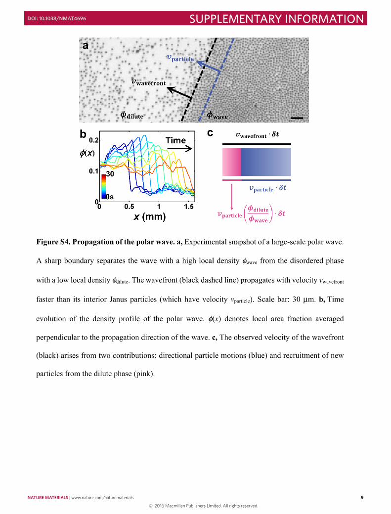
Supplementary Fig. S4a illustrates a typical propagating polar flow. A distinct wavefront
is observed, which separates the dilute, disordered region (with area fraction φdilute) and the dense,
swarming region (with area fraction φwave). Based on the PIV analysis (see main text), the
wavefront propagates at a speed vwavefront ≈ 40 µm/s, 1.3-1.4 times faster than the swimming Janus
particles (with speed vparticle = 29 µm/s in this case) inside the polar flow. To explain this speed
difference, we observe that the propagation velocity of a polar wave originates from two
contributions, the directional particle motion and the recruitment of particles from the dilute phase.
Within an infinitesimal time step δt, a particle within the traveling wave travels a distance vparticleδt.
Meanwhile, the disordered phase has an average velocity of zero in the lab reference frame; hence,
the Janus particles in the dilute phase move with an average speed −vparticle relative to the wave.
Physically, these particles accumulate at the wavefront and once they reach the wavefront they
reorient and become part of the wave. The total number of particles joining the wave is
proportional to φdilute⋅vparticleδt. As a consequence, the wavefront translates by
(1+φdilute/φwave)⋅vparticleδt, and hence vwavefront = (1+φdilute/φwave)⋅vparticle. Using representative numbers
from Supplementary Fig. S4b, for example φdilute = 0.03 and φwave = 0.12 at t = 10 s, we estimate
the ratio between the wavefront velocity and the particle velocity to be 1.25, close to the observed
value.
8 NATURE MATERIALS | www.nature.com/naturematerials
SUPPLEMENTARY INFORMATION DOI: 10.1038/NMAT4696
© 2016 Macmillan Publishers Limited. All rights reserved.
9
Figure S4. Propagation of the polar wave. a, Experimental snapshot of a large-scale polar wave.
A sharp boundary separates the wave with a high local density φwave from the disordered phase
with a low local density φdilute. The wavefront (black dashed line) propagates with velocity vwavefront
faster than its interior Janus particles (which have velocity vparticle). Scale bar: 30 µm. b, Time
evolution of the density profile of the polar wave. φ(x) denotes local area fraction averaged
perpendicular to the propagation direction of the wave. c, The observed velocity of the wavefront
(black) arises from two contributions: directional particle motions (blue) and recruitment of new
particles from the dilute phase (pink).
NATURE MATERIALS | www.nature.com/naturematerials 9
SUPPLEMENTARY INFORMATIONDOI: 10.1038/NMAT4696
© 2016 Macmillan Publishers Limited. All rights reserved.
10
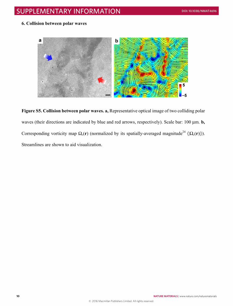
6. Collision between polar waves
Figure S5. Collision between polar waves. a, Representative optical image of two colliding polar
waves (their directions are indicated by blue and red arrows, respectively). Scale bar: 100 µm. b,
Corresponding vorticity map Ωz(r) (normalized by its spatially-averaged magnitude24 〈|Ωz(r)|〉).
Streamlines are shown to aid visualization.
10 NATURE MATERIALS | www.nature.com/naturematerials
SUPPLEMENTARY INFORMATION DOI: 10.1038/NMAT4696
© 2016 Macmillan Publishers Limited. All rights reserved.

11
7. Time evolution in the cluster phase
Figure S6. Time evolution in the cluster phase. a, Snapshots of cluster formation of Janus
particles in an 0.1 mM NaCl solution acted upon by a 10 V, 40 kHz AC electric field. Scale bar
100 µm. b, Illustrative additional snapshots showing the coarsening process on a finer scale.
Clusters grow primarily by merger (red circles) during the first 60 seconds, but during the
following 75 seconds primarily via a process akin to Ostwald ripening in which swimming
particles leave small clusters (blue circle) and join larger ones (red circle). Scale bar 40 µm.
NATURE MATERIALS | www.nature.com/naturematerials 11
SUPPLEMENTARY INFORMATIONDOI: 10.1038/NMAT4696
© 2016 Macmillan Publishers Limited. All rights reserved.

12
8. Analytical estimate of the stability limit of the chain state
Figure S7. Representative head-to-tail configuration of two Janus particles in a chain.
In the chain state, Janus colloids concatenate by forming a head-to-tail configuration. Here
we analytically estimate the phase boundaries of this state. As a first approximation, to stabilize a
chain configuration, the overall dipolar force between two adjacent Janus particles (Supplementary
Fig. S7), i.e., the sum of four pairwise forces between their head dipoles µhead and tail dipoles µtail,
should be attractive. We calculate the total force between the two particles as
F = − 3
4πε0µhead2
2a( )4+
µtail2
2a( )4+
µheadµtail2a+2d( )4
+µheadµtail2a−2d( )4
⎡
⎣
⎢⎢
⎤
⎦
⎥⎥
,
where the dipole shift d = (3/8)a. By setting F = 0, we solved this quadratic equation to give
µtail/µhead = −6.7 or −0.15, the estimated upper and lower boundaries. The actual span observed in
the simulations (−5, −0.35) is close to this estimate.
12 NATURE MATERIALS | www.nature.com/naturematerials
SUPPLEMENTARY INFORMATION DOI: 10.1038/NMAT4696
© 2016 Macmillan Publishers Limited. All rights reserved.

13
9. Comparison between simulation and experiment
To compare the experimental observations with the phase diagram obtained in simulation
(Fig. 4 in the main text), we need to convert the complex dipole coefficient K into a real number.
We proceed by calculating the dipolar interaction. For two hemispheres A and B, the interaction
is
UAB =
4πε0εsRe KA∗KB( )a6E02
rAB3 ,
where E0 is the amplitude of the applied field and rAB the distance between their induced dipoles.
We set rAB = 2a to calculate the interaction pairs Uhead−head and Utail−tail, and use Utail−tail Uhead−head
(taking appropriate account of the sign) as an estimate for µtail/µhead. To obtain the experimental
swimming force Fswim, we track the average velocity v of swimming Janus spheres, and estimate
the force as Fswim = 6πηav. Such calculations yield R = µtail/µhead equal to 0.1, 1.7 and −0.5 and
M = Frep/Fswim equal to 15, 3, 22 for the swarming, isotropic and chaining states, respectively, in
agreement with the simulation phase diagram. However, the clustering phase observed in
experiment corresponds to a dipole ratio µtail/µhead = 1.9, lower than the phase boundary predicted
by the simulation. In reality, the imaginary part of the dipole coefficients gives rise to a moderate
attraction between head and tail hemispheres. This aids particle aggregation by forming short,
transient chains and thus reduces the requirement for the electrostatic imbalance µtail/µhead.
Nevertheless, for simplicity and generality, we use real-valued dipoles in the simulations.
NATURE MATERIALS | www.nature.com/naturematerials 13
SUPPLEMENTARY INFORMATIONDOI: 10.1038/NMAT4696
© 2016 Macmillan Publishers Limited. All rights reserved.

14
Supplementary References
31. Sharma, V., Yan, Q., Wong, C. C., Carter, W. C. & Chiang, Y.-M. Controlled and rapid
ordering of oppositely charged colloidal particles. J. Colloid Interface Sci. 333, 230-236
(2009).
32. Shilov, V. N., Delgado, A. V., Gonzalez-Caballero, F. & Grosse, C. Thin double layer
theory of the wide-frequency range dielectric dispersion of suspensions of non-conducting
spherical particles including surface conductivity of the stagnant layer. Colloids Surf. A
192, 253-265 (2001).
33. Boero, M., Ikeshoji, T. & Terakura, K. Density and temperature dependence of proton
diffusion in water: A first-principles molecular dynamics study. ChemPhysChem 6, 1775-
1779 (2005).
34. Zeebe, R. E. On the molecular diffusion coefficients of dissolved CO2, HCO3", and CO3
2"
and their dependence on isotopic mass. Geochim. Cosmochim. Acta 75, 2483-2498 (2011).
35. Samson, E., Marchand, J. & Snyder, K. A. Calculation of ionic diffusion coefficients on
the basis of migration test results. Mat. Struct. 36, 156-165 (2003).
36. Garcia-Sánchez, P., Ren, Y., Arcenegui, J. J., Morgan, H. & Ramos, A. Alternating current
electrokinetic properties of gold-coated microspheres. Langmuir 28, 13861-13870 (2012).
37. Pascall, A. J. & Squires, T. M. Induced charge electro-osmosis over controllably
contaminated electrodes. Phys. Rev. Lett. 104, 088301 (2010).
14 NATURE MATERIALS | www.nature.com/naturematerials
SUPPLEMENTARY INFORMATION DOI: 10.1038/NMAT4696
© 2016 Macmillan Publishers Limited. All rights reserved.
15
38. Kijlstra, J., van Leeuwen, H. P. & Lyklema, J. Low-frequency dielectric relaxation of
hematite and silica sols. Langmuir 9, 1625-1633 (1993).
39. Suzuki, R., Jiang, H. R. & Sano, M. Validity of fluctuation theorem on self-propelling
particles. arXiv:1104.5607 (2011).
NATURE MATERIALS | www.nature.com/naturematerials 15
SUPPLEMENTARY INFORMATIONDOI: 10.1038/NMAT4696
© 2016 Macmillan Publishers Limited. All rights reserved.

16
Titles and legends for Supplementary Movies
Supplementary Movie 1: Active chain state in 3D simulations. This movie shows growing chains
of Janus particles (volume fraction 0.0077) in a 3D molecular dynamics simulation 30 seconds
after swimming is initiated. A constant force is applied as described in Methods section to each
particle, which carries a negative charge −200e on its leading hemisphere and a positive charge
+200e on its trailing hemisphere. The movie is played 3× faster than real time and lasts 45 seconds
in real units.
Supplementary Movie 2: Active swarm state in 3D simulations. This movie shows growing
swarms of Janus particles (volume fraction 0.0157) in a 3D molecular dynamics simulation just
after swimming is initiated. A constant force is applied as described in Methods section to each
particle, which carries a strongly charged leading hemisphere (−2500e) and a neutral trailing
hemisphere. The movie is played 2× faster than real time and lasts 34 seconds in real units.
Supplementary Movie 3: Active cluster state in 3D simulations. This movie shows growing
clusters of Janus particles (volume fraction 0.0077) in a 3D molecular dynamics simulation just
after swimming is initiated. A constant force is applied as described in Methods section to each
particle, which has a neutral leading hemisphere and a highly charged trailing hemisphere
(+1000e). The movie is played 3× faster than real time and lasts 24 seconds in real units.
Supplementary Movie 4: Homogeneous (“active gas”) state in quasi-2D experiment. This movie
shows Janus colloids (3 µm diameter), sedimented to the bottom of a sample cell in water,
swimming in response to an electric field of 7 V and 5 kHz perpendicular to the image plane. The
movie plays in real time. The viewing window is 95 ⋅ 127 µm2.
16 NATURE MATERIALS | www.nature.com/naturematerials
SUPPLEMENTARY INFORMATION DOI: 10.1038/NMAT4696
© 2016 Macmillan Publishers Limited. All rights reserved.

17
Supplementary Movie 5: Representative collision-induced alignment event of head-repulsive
particles observed in quasi-2D experiment. This movie shows two colliding swimmers,
highlighted by blue circles, swimming in response to an electric field (10 V, 30 kHz) perpendicular
to the image plane. The movie plays 3× slower than real time. The viewing window is 80 ⋅ 80 µm2.
Supplementary Movie 6: Swarm state observed in quasi-2D experiment after swimming is initiated.
This movie shows particles sedimented to the bottom of a sample cell in water, stimulated to swim
in an electric field (10 V, 30 kHz) perpendicular to the image plane. The movie plays in real time.
The viewing window is 64 ⋅ 80 µm2.
Supplementary Movie 7: Active chain state observed in quasi-2D experiment after swimming is
initiated. This movie shows particles sedimented to the bottom of a sample cell in water, stimulated
to swim in an electric field of 10 V and 1 MHz. Note the mixture of growing chains and rings,
with the formation of a stationary rotating ring near the end of the movie. The movie plays in real
time. The viewing window is 46 ⋅ 60 µm2.
Supplementary Movie 8: Active clustering observed in quasi-2D experiment after swimming is
initiated. This movie shows Janus particles sedimented to the bottom of a sample cell in an 0.1 mM
NaCl solution and stimulated to swim in an electric field (10 V, 40 kHz) perpendicular to the image
plane. The movie plays 20× faster than real time. The viewing window is 380 × 506 µm2.
Supplementary Movie 9: Polar wave observed in quasi-2D experiment. This movie shows the
formation of propagating wave of collectively swarming Janus colloids observed with a 5⋅
objective within a large view window of 1215 ⋅ 1620 µm2 while swimming in an electric field
(10 V, 30 kHz) perpendicular to the image plane. The first half of the movie, played at 4× real
NATURE MATERIALS | www.nature.com/naturematerials 17
SUPPLEMENTARY INFORMATIONDOI: 10.1038/NMAT4696
© 2016 Macmillan Publishers Limited. All rights reserved.

18
time, demonstrates the evolution from small swarms into a large polar wave. The second half,
played at 4× real time, shows a shock wave sweeping over the field of view at a later stage.
Supplementary Movie 10: Vortex observed in quasi-2D experiment. This movie shows a giant
vortex formed in the late stage of the swarm state, for particles sedimented to the bottom of a
sample cell and swimming in an electric field (10 V, 30 kHz) perpendicular to the image plane.
The movie plays 6× faster than real time. The viewing window is 1215 ⋅ 1620 µm2.
18 NATURE MATERIALS | www.nature.com/naturematerials
SUPPLEMENTARY INFORMATION DOI: 10.1038/NMAT4696
© 2016 Macmillan Publishers Limited. All rights reserved.