This content has been downloaded from IOPscience. Please scroll down to see the full text.

Download details:

IP Address: 132.170.150.82

This content was downloaded on 14/02/2014 at 17:22

Please note that terms and conditions apply.

Reconstructing small perturbations in electrical admittivity at low frequencies

View the table of contents for this issue, or go to the journal homepage for more

2014 Inverse Problems 30 035006

(http://iopscience.iop.org/0266-5611/30/3/035006)

Home Search Collections Journals About Contact us My IOPscience

Inverse Problems

Inverse Problems 30 (2014) 035006 (18pp) doi:10.1088/0266-5611/30/3/035006

Reconstructing small perturbations inelectrical admittivity at low frequencies

Sungwhan Kim1 and Alexandru Tamasan2

1 Division of Liberal Arts, Hanbat National University, Korea2 Department of Mathematics, University of Central Florida, USA

E-mail: sungwhan@hanbat.ac.kr and tamasan@math.ucf.edu

Received 19 August 2013, revised 25 December 2013Accepted for publication 7 January 2014Published 12 February 2014

AbstractWe present a method to recover small perturbations from constants in electricalconductivity σ and relative (to the air’s) permittivity ε of a body, from electricalmeasurements at low frequencies at the boundary. The method is based onthe asymptotic expansion of the frequency differential of the Neumann-to-Dirichlet map with respect to both frequency and perturbation size. To showits feasibility, we implement the method on two numerical experiments for acomplete electrode model.

Keywords: electrical impedance tomography, small perturbation, frequencydifferential

(Some figures may appear in colour only in the online journal)

1. Introduction

Electrical impedance tomography (EIT) is the imaging technique in which the electricalconductivity σ and permittivity ε of a body � is to be recovered from knowledge of electricalcurrents and voltages at its boundary �. In this study we have in mind excitations at lowfrequency ν of order of 1 kHz. In the imaginary part of the admittivity σ + iνε we assume apermittivity ε scaled relative to the permittivity εair of air, i.e.

ε := ε/εair, ω := νεair.

Since εair ≈ 8.8 × 10−12 F m−1 and ν ≈ 1 kHz, the values of ω are numerically small of orderO(10−8). Note that the susceptivity νε is invariant under this scaling.

Most generally formulated by Calderon [8] at ω = 0 (when only σ has been sought), theproblem has seen a tremendous development both on the mathematics and engineering facetwith breakthrough results in [1, 7, 25, 26, 27, 37] complemented by important contributionsas reviewed in [2, 4, 9, 15, 39]. At zero frequency direct nonlinear approaches that use the

0266-5611/14/035006+18$33.00 © 2014 IOP Publishing Ltd Printed in the UK 1

Inverse Problems 30 (2014) 035006 S Kim and A Tamasan

complex geometrical optic solutions (CGOs) have been proposed in [21, 23, 24, 30] basedon the reconstruction methods in [1, 3, 6, 22, 27]. At a fixed frequency ω, the Dirichlet-to-Neumann map uniquely determines the admittivity σ + iνε. This is true in dimensions 2 due tothe result in [7], also in [10] for sufficiently small susceptivity νε. Note that we do not assumea small susceptivity here since the scaling above leaves the susceptivity invariant.

In three dimensions and higher the results in [26, 37] seem to extend to the complexcoefficient case provided a priori information on admittivity and its normal derivative at theboundary is known. An algorithm for two dimensional complex admittivity based on [10] hasbeen proposed recently in [11].

At low frequencies the effect of susceptivity cannot be neglected and working with acomplex valued voltage potential becomes necessary. Practitioners are able to measure boththe magnitude and the phase of the complex valued potential at the boundary [5, 28, 31, 36,38]. At low frequencies the information about permittivity is mainly carried by the imaginarypart of the voltage potential [20]. The results in section 2 (see remark 2.3) identifies the neededinformation and how it can be obtained in two different ways:

– on the one hand one can use the real part of a suitably scaled voltage potential. This is theapproach we took in the numerical experiments here;

– on the other hand one can use the difference in voltages at two distinct frequencies. Thisis a fairly recent development known as the frequency difference/differential EIT (fdEIT)[12, 13, 16, 18, 19, 33, 34].

In general, the methods based on subtraction of two boundary data seem to be more robustdue to the cancellation of instrumentation errors in the data; this has also been observed infdEIT [33, 34].

We work under the assumptions that σ = σ (x) and ε = ε(x). In reality they also varywith frequency ω. For data collected at a single frequency this work interprets the conductivityand permittivity as the ones corresponding to that single frequency. For data collected at twodifferent but comparable frequencies, we assume that σ and ε do not vary with frequency atcomparable values.

The mathematical formulation considers a time harmonic current gcos(ωt) being injectedinto an object � through surface electrodes to induce a complex voltage potential uω solutionof the Neumann problem:⎧⎪⎨

⎪⎩∇ · (σ + iωε)∇uω = 0, in �,

−(σ + iωε) ∂uω

∂n = g, on �,∫�

uω ds = 0,

(1)

for some real valued function g ∈ H−1/2(�). Assuming 1/c � σ � c for some c > 0, theunique solution uω of (1) is measured at the boundary to define the Neumann-to-Dirichlet mapNγω

: H−1/20 (�) → H1/2

0 (�) by

Nγω: g �→ uω|�. (2)

Here H1/20 (�) is the space of traces with vanishing mean at the boundary of functions in

H1(�), and H−1/20 (�) is the dual of H1/2

0 (�) with respect to the L2(�)-inner product.Despite the transparent usefulness in medical diagnostics, the quantities behind the fdEIT

images are not yet fully understood. However, for � ⊂ Rn, n � 3, σ ∈ C1,1(�) constant near

the boundary and ε ∈ C1,10 (�) the frequency differential at ω = 0 of the Dirichlet-to-Neumann

map uniquely determines the quantity

Q[σ, ε] := ∇ · (∇ε − ε∇ ln σ )/σ (3)

2

Inverse Problems 30 (2014) 035006 S Kim and A Tamasan

as shown by the authors in [20]. The method is non-constructive and relies on CGOs. Sinceknowledge of the Dirichlet-to-Neumann map is equivalent to knowledge of the Neumann-to-Dirichlet map, one can conclude that the quantity Q is also uniquely determined by d

dω

∣∣ω=0

Nγω.

In this paper we give a reconstruction method for the linearized problem of fdEIT aboutsome known constant conductivity σb, and permittivity εb, which quantitatively recovers theperturbations. The method proposed is not based on CGOs and applies to models in two orhigher dimensions. To exhibit the error estimates due to the linearization, we consider

σt := σb + tσ , εt := εb + t ε, γ tω := σt + iωεt, (4)

for some σ , ε ∈ L∞(�) with compact support in �, and t � 0 sufficiently small. While σ andε are not known, we assume they are a priori bounded by some known r � 0:

‖σ‖∞ � r and ‖ε‖∞ � r, (5)

where ‖ · ‖∞ denotes the L∞(�)-norm.Since (σ , ε)|� are assumed known (in fact vanishing), the derivative

dQ[σt, εt]

dt

∣∣∣∣t=0+

= εb

σb�

(ε

εb− σ

σb

),

recovers the quantity

δQ :=(

ε

εb− σ

σb

). (6)

For sufficiently small t, in here we reconstruct t[δQ] from the frequency differential ofan appropriately scaled Nγ t

ω. The method is based on the following result, which is proved in

section 3.

Theorem 1.1. Let σt, εt , and γ tω in (4) satisfy (5). Let t0 � 1 be sufficiently small such that

1/c � σt � c, (7)

for some c > 0 independent of 0 � t � t0. Let f , g ∈ H−1/20 (�), and φ f , φg ∈ H1(�)

be the harmonic functions with mean vanishing traces on �, which satisfy −σb∂φ f

∂n

∣∣�

= f ,

respectively −σb∂φg

∂n

∣∣�

= g . Then, with δQ the quantity in (6), we have∫�

[δQ]∇φg · ∇φ f dx = limt→0+

1

t

⟨d

dω

∣∣∣∣ω=0

{(ω

σb− i

εb

)Nγ t

ωg

}, f

⟩�

, (8)

where 〈·, ·〉� denotes the pairing of functions in H±1/2(�) with respect to the L2(�)-innerproduct.

Since products of gradients of harmonic function is dense in L2(�) (as originally notedby Calderon in his linearization approach in [8]), the right-hand side of (8) for appropriatechoices of f and g uniquely determines (the Fourier transform of) δQ in (6). However, in themethod proposed here we do not use the density of gradients of harmonic functions above.Instead, we propose a method in which the resolution in the image is predetermined by thenumber (of combinations) of electrodes, where in each pixel the unknown δQ is assumedconstant. The method and its numerical implementation are tailored for the complete electrodemodel in [35].

While the nonlinear approach in [20] shows that ddω

∣∣ω=0

Nγωrecovers Q, in here we

show that the linearization of ddω

∣∣ω=0

Nγωrecovers the linearization of Q. This gives a natural

interpretation of (6), whose support has been recovered previously in [12].A key feature of authors’ result in [20] is the analytic dependence in ω of the voltage

potential, for frequencies satisfying∥∥∥ωε

σ

∥∥∥∞

< 1, (9)

3

Inverse Problems 30 (2014) 035006 S Kim and A Tamasan

which allows for a recurrence type decoupling in the real and imaginary part of uω. Theanalogous result (proven in the appendix) holds for the solution of the Neumann problem (1),and allows to explicit the asymptotic expansion of the data d

dω

∣∣ω=0

{(ωσb

− iεb

)Nγ t

ωg}

with anerror estimate; it also explains why the harmonic functions appearing in the left-hand sideof (8) are independent on the permittivity. The hypothesis (9) is meaningful to biomedicalapplications such as in [32]. According to experimental values at 10 kHz for a variety ofbiological tissues [29], the left-hand side of (9) has a maximum of 0.528 achieved in the tissueof the heart.

In section 4 we present a method which reconstructs t(δQ) from boundary voltages. Weuse the complete electrode model in [35] to obtain (approximate) solutions of the Neumannproblem (1).

In section 5 we first adapt Calderon’s original arguments to recover the small perturbationtσ from the real part �(uω). In combination with knowledge of t(δQ) we can also recover t εseparately. Different from the result in [14], which recovers the support of the perturbation inadmittivity, our method here provides a quantitative reconstruction.

The method is implemented in two numerical experiments in section 6. We conclude witha series of remarks.

2. Analytic dependence in frequency

In this section we present the analytic dependence in ω of the complex valued solutionsuω ∈ H1(�) of (1). The admittivity need not be a small perturbation from constant. Due tothe frequency dependence in the Neumann boundary condition the estimates (while similarto the ones in [20, theorem 3.1]) requires a different proof. To preserve the flow of expositionof the inverse problem, the details are included in the appendix.

Theorem 2.1. Let σ, ε ∈ L∞(�) with σ satisfying (7) for some c > 0. Assume that ω lies inthe frequency range (9). Then the Neumann problem (1) has a unique solution uω ∈ H1(�),whose real part vω = �(uω), and imaginary part hω = (uω) satisfy the series representation

vω(x) =∞∑

n=0

v2n(x)ω2n, hω(x) =∞∑

n=0

h2n+1(x)ω2n+1, (10)

with the convergence in the H1(�)-sense. Moreover, v0 solves⎧⎪⎨⎪⎩

∇ · (σ∇v0) = 0, in �,

−σ ∂v0∂n = g, on �,∫

�v0 ds = 0,

(11)

and, for k = 0, 1, 2, . . . , the following recurrences hold:⎧⎪⎪⎪⎪⎪⎪⎨⎪⎪⎪⎪⎪⎪⎩

∇ · (σ∇h2k+1) = −∇ · (ε∇v2k), in �,

∇ · (σ∇v2k+2) = ∇ · (ε∇h2k+1), in �,

−σ∂h2k+1

∂n = (−1)k+1(

εσ

)2k+1g, on �,

−σ∂v2k+2

∂n = (−1)k+1(

εσ

)2k+2g, on �,∫

�v2k+2 ds = ∫

�h2k+1 ds = 0.

(12)

As a corollary, we can now clarify the operator appearing in the right-hand side of (8).

4

Inverse Problems 30 (2014) 035006 S Kim and A Tamasan

Corollary 2.2. Let σ, ε ∈ L∞(�), with 1/c � σ � c, for some c > 0. For g ∈ H1/2(�) realvalued we have

d

dω

∣∣∣∣ω=0

{(ω

σb− i

εb

)Nγω

g

}= v0

σb+ h1

εb, (13)

where v0 ∈ H1(�) solves (11), and h1 solves⎧⎪⎨⎪⎩

∇ · (σ∇h1) = −∇ · (ε∇v0), in �,

σ ∂h1∂n = (

εσ

)g, on �,∫

�h1 ds = 0.

(14)

Proof. From theorem 2.1 a straightforward calculation shows that(ω

σb− i

εb

)Nγω

g = −iv0

εb+ ω

(v0

σb+ h1

εb

)+ ω2R(ω). (15)

Moreover, a geometric series summation using the estimates (A.7) and (A.8) in the appendixshow that

|R(ω)|1/2 � M||g‖−1/2

∥∥∥ ε

σ

∥∥∥2

∞

(1 −

∥∥∥εω

σ

∥∥∥∞

)−1, (16)

for a constant M which depends on c and � only. �Recall that at low frequencies we work with ω = O(10−8). The following note explains

what information obtained from the voltage potential at the boundary is needed in ourlinearization approach.

Remark 2.3. From the asymptotic formula (15), the right-hand side of (13) can be recoveredfrom boundary data in two different ways:

• For ω1, ω2 = O(ω) with ω1 �= ω2 one can use a difference quotient to getv0

σb+ h1

εb= 1

ω2 − ω1

[(ω

σb− i

εb

)Nγω

g

]ω2

ω1

+ O(ω). (17)

• Upon one division by ω and then taking the real part in (15), we havev0

σb+ h1

εb= �

{(1

σb− i

ωεb

)Nγω

g

}+ O(ω). (18)

In fdEIT one would use the boundary data as in (17). In the numerical experiments insection 6, we use the formula (18).

3. Proof of theorem 1.1

In this section we denote by ‖ · ‖±1/2 the norm in H±1/2(�), by ‖ · ‖±1 the norm in H±1(�),and by ‖ · ‖ the norm in L2(�). We make use several times of the classical estimate in theNeumann problem, which we state without proof below.

Proposition 3.1. Let F ∈ H−1(�), g ∈ H−1/20 (�) and σ ∈ L∞(�) satisfying (7) for some

c > 0. Let v ∈ H1(�) be the unique solution of the Neumann problem⎧⎪⎨⎪⎩

∇ · (σ∇v) = F, in �,

−σ ∂v∂n = g, on �,∫

�v ds = 0.

Then there exists a constant M > 0, dependent only on � and c, such that

‖v‖1 � M(‖g‖−1/2 + ‖F‖−1). (19)

5

Inverse Problems 30 (2014) 035006 S Kim and A Tamasan

To simplify notation, for the rest of the proof in this section we will drop the vanishingmean normalizing condition from the Neumann problems below, although it is always tacitlyassumed.

Recall the notations in (4), and the fact that σt satisfies (7) for a constant c > 0 independentof 0 � t � t0. By possibly replacing the constant c by εb + r, without loss of generality wealso assume

‖εt‖∞ � c, for 0 � t � t0 � 1. (20)

Since we no longer use the series but rather the formula (13), and in order to emphasizedependence in t without cluttering notation, we let vt ∈ H1(�) denote the solutions to{∇ · (σt∇vt ) = 0, in �,

−σt∂vt∂n = g, on �,

(21)

and ht ∈ H1(�) denote the solution of{∇ · (σt∇ht ) = −∇ · (εt∇vt ), in �,

σt∂ht∂n = εt

σtg, on �.

(22)

Then, according to (13),

d

dω

∣∣∣∣ω=0

(ω

σb− i

εb

)Nγ t

ωg =

(vt

σb+ ht

εb

). (23)

For g, f ∈ H1/2 recall that φg, φ f are the harmonic functions with traces of vanishingmean on � that satisfy the Neumann conditions −σb

∂φg

∂n = g, respectively −σb∂φ f

∂n = f . Notethat φg solves (21) when t = 0. Also, let h0 be the solution of (22) for t = 0, i.e., h0 is theharmonic function with trace of vanishing mean on �, which satisfies the Neumann conditionσb

∂h0∂n = εb

σbg, in particular we have

h0 = − εb

σbφg. (24)

Next we use the estimates (19) in the forward problem to exhibit the t-asymptotic(with t → 0+) of the left-hand side of (13).

In all the estimates below the constant M may change from equation to equation, but atall times remains a constant dependent only on the domain �, the ellipticity constant c > 0,and, for brevity, on the constants σb and εb. Dependence on r > 0 in (5) will remain explicit.

By proposition 3.1 applied to (21) we obtain

max{‖vt‖1, ‖φg‖1} � M‖g‖−1/2, (25)

and when applied to (22) we obtain

‖ht‖1 � M

(‖∇ · εt∇vt‖−1 +

∥∥∥∥ εt

σt

∥∥∥∥∞

‖g‖−1/2

)� M‖εt‖∞(‖∇vt‖ + c‖g‖−1/2)

� M(‖vt‖1 + ‖g‖−1/2) � M‖g‖−1/2, (26)

where the last inequality uses (25).Now let

δv := vt − φg, and δh := ht − h0. (27)

A simple calculation shows that (δv) solves{∇ · σt∇(δv) = −t∇ · σ∇φg, in �,

σt∂(δv)

∂n = tσ ∂φg

∂ν, on �.

6

Inverse Problems 30 (2014) 035006 S Kim and A Tamasan

By proposition 3.1 we estimate

‖δv‖1 � tM

(‖∇ · σ∇φg‖−1 +

∥∥∥∥σ∂φg

∂ν

∥∥∥∥−1/2

)

� tM‖σ‖∞(‖∇φg‖ + ‖g‖−1/2)

� tMr‖g‖−1/2, (28)

where the last inequality uses (5) and (25).To estimate (δh) in (27), we note first that it solves{∇ · σb∇(δh) = −∇ · (tσ∇ht − εt∇(δv) − t ε∇φg), in �

σb∂(δh)

∂n = −t σ εt

σ 2t

g + (εtσt

− εbσb

)g, on �.

(29)

Also, by using (7) and (5) we have∣∣∣∣ εt

σt− εb

σb

∣∣∣∣ = t

∣∣∣∣σbε − εbσ

σtσb

∣∣∣∣ � trc

(1 + εb

σb

). (30)

By applying once more proposition 3.1 to (29) we estimate

‖δh‖1 � M

(t‖σ‖∞‖∇ht‖ + ‖εt‖∞‖∇(δv)‖ + t‖ε‖∞‖∇φg‖

+∥∥∥∥ σ εt

σ 2t

∥∥∥∥∞

‖g‖−1/2 + trc

(1 + εb

σb

)‖g‖−1/2

)� tMr‖g‖−1/2, (31)

where in the last inequality we used in the estimates (26), (28), (25), and (30) in this order.We have now all the ingredients necessary to establish (8). We start by multiplying the

top equation of (22) by φ f , and use Green’s formula once to obtain∫�

σt∂ht

∂νφ f ds −

∫�

σt∇ht∇φg = −∫

�

εt∂vt

∂νφ f ds +

∫�

εt∇vt · ∇φ f dx.

Now use the Neumann condition in (22) and (21) to cancel the two boundary integrals aboveand obtain the key identity∫

�

(σt∇ht + εt∇vt ) · ∇φ f dx = 0. (32)

In the identity (32) we first replace σt = σb + tσ , εt = εb + t ε, and separate the zero orderterms to get ∫

�

(σb∇ht + εb∇vt ) · ∇φ f dx = −t∫

�

(σ∇ht + ε∇vt ) · ∇φ f dx.

Now use ht = h0 + (δh), and vt = φg + (δv) and further separate the first order from thequadratic terms in the right-hand side above. Upon one division by εbσb we obtain∫

�

(1

εb∇ht + 1

σb∇vt

)· ∇φ f dx = − t

εbσb

∫�

(σ∇h0 + ε∇φg) · ∇φ f dx − t2r2R(t), (33)

where r is the bound in (5) and the remainder

R(t) := 1

tr2σbεb

∫�

[σ∇(δh) + ε∇(δv)] · ∇φ f dx. (34)

Using the H1(�)-estimates of (δv) in (28) and of (δh) in (31), it is easy to see the uniformbound

|R(t)| � M‖g‖−1/2‖ f ‖−1/2, (35)

for some constant M dependent only on �, c, σb and εb.

7

Inverse Problems 30 (2014) 035006 S Kim and A Tamasan

Returning to (33), we use Green’s identity in the left-hand side, and the relation (24)between h0 and φg to get∫

�

f

(ht

εb+ vt

σb

)ds = t

∫�

(σ

σb− ε

εb

)∇φg∇φ f dx − t2r2R(t). (36)

Finally, corollary 2.2 in the formula (23) identifies the left-hand side in (36) to concludethe t-asymptotic expansion⟨

f ,d

dω

∣∣∣∣ω=0

(ω

σb− i

εb

)Nγ t

ωg

⟩= t

∫�

[δQ]∇φg∇φ f dx − t2r2R(t). (37)

This proves theorem 1.1.

4. A reconstruction method for δQ using the complete electrode model

Recall the notations in (4)

σt := σb + tσ , εt := εb + t ε, γ tω := σt + iωεt,

for some known constants σb, εb, and unknown σ , ε ∈ L∞(�) of compact support in �. Weassume the a priori bound in (5) holds for some r > 0.

In this section we first propose a method based on theorem 1.1 to approximately reconstruct

t[δQ] =(

t ε

εb− tσ

σb

),

for t sufficiently small.The method uses the complete electrode model [35] as follows. Let L electrodes e1, . . . , eL

of corresponding impedance ζ1, . . . , ζL be placed at the boundary �. In each experiment weuse a pair of electrodes, say (el, e j) to inject/extract a time harmonic current Il j cos ωt. Thereare L(L − 1)-many experiments as (l, j) ranges in {1, . . . , L} × {1, . . . , L} with l �= j. Thecomplete electrode model (if γ t

ω were known) assumes the complex voltage potential ul jω would

distribute inside according to the problem⎧⎪⎪⎪⎪⎪⎪⎨⎪⎪⎪⎪⎪⎪⎩

∇ · (γ tω∇ul j

ω

) = 0, in �,(ul j

ω + ζlγtω

∂ul jω

∂n

)∣∣∣el

≡ const. ≡ −(

ul jω + ζ jγ

tω

∂ul jω

∂n

)∣∣∣e j

− ∫el

γ tω

∂ul jω

∂n ds = ∫e j

γ tω

∂ul jω

∂n ds = Il j

−γ tω

∂ul jω

∂n = 0, on � \ {e j ∪ el}.

(38)

The voltage potential ul jω also solves the Neumann problem (1) with the Neumann boundary

data given by

gl j := −γ tω

∂ul jω

∂n

∣∣∣∣∣�

. (39)

We note here that point-wise values of gl j are unknown on the electrodes el , e j.At each electrode ek not used in injection we measure Ul j

ω,k, which gives∫ek

ul jω ds = Ul j

ω,k, k �= l, j. (40)

8

Inverse Problems 30 (2014) 035006 S Kim and A Tamasan

At the electrode el where we ‘inject’ we may measure Ul jω,l , which yields∫

el

ul jω ds = Ul j

ω,l + ζl Il j. (41)

Similarly at the electrode e j where we ‘extract’ we may measure Ul jω, j, which yields∫

e j

ul jω ds = Ul j

ω, j − ζ jIl j. (42)

Now theorem 2.1 yields the asymptotic

ul j = vl j0 + iωhl j

1 + O(ω2).

By taking the real part and integrating over ek in (15), and using the measured data in (40) weobtain ∫

ek

(v

l j0

σb+ hl j

1

εb

)ds = �

{(1

σb− i

εbω

) (Ul j

ω,k + δl jk ζkIl j

)} + O(ω), (43)

where

δl jk =

⎧⎨⎩

1, if k = l,−1, if k = j,0, if k �= l, j.

(44)

By using the t-asymptotic in (36) we obtain for an arbitrary f ∈ H−1/2(�) that∫�

t[δQ]∇φgl j∇φ f dx =∫

�

(v

l j0

σb+ hl j

1

εb

)f ds + t2r2R(t), (45)

where φgl j , φ f are the harmonic functions with traces of vanishing mean on � that satisfy theNeumann conditions

−σb∂φgl j

∂n= gl j, −σb

∂φ f

∂n= f .

Recall that gl j is not known point-wise on the electrodes el and e j. We use instead anapproximate φl j solution to⎧⎪⎪⎪⎪⎪⎨

⎪⎪⎪⎪⎪⎩

�φgl j = 0, in �,

−σb∂φgl j

∂n = 1|el | Il j, on el,

−σb∂φgl j

∂n ds = − 1|e j | Il j, on e j

−σb∂φgl j

∂n = 0, on � \ (el ∪ e j).

(46)

Note that the choice of f ∈ H−1/2(�) is totally free. We choose f supported on theelectrodes and constant on each electrode. For an arbitrary α = (α1, . . . , αL) ∈ R

L, withα1 + α2 + · · · + αL = 0, let

fα =L∑

k=1

αkχek , (47)

where χek denotes the characteristic function of ek.By using (43) into (45) we obtain the system of equations∫

�

t[δQ]∇φgl j∇φ fα dx =L∑

k=1

αk�{(

1

σb− i

εbω

)(Ul j

ω,k + δl jk ζkIl j)

}+ t2r2R(t) + ωR(ω),

(48)

9

Inverse Problems 30 (2014) 035006 S Kim and A Tamasan

where δl jk is given by (44). Moreover, according to (35), we have the error estimate

|R(t)| � M‖gl j‖−1/2‖ f ‖−1/2,

(M depends only on �, c, σb, and εb), and following from (16),

|R(ω)| � N∥∥∥ ε

σ

∥∥∥2

∞

(1 −

∥∥∥εω

σ

∥∥∥∞

)−1‖gl j‖−1/2‖ f ‖−1/2, (49)

for some constant N which depends on c only.For t and ω sufficiently small we use the linear approximation∫

�

t[δQ]∇φgl j∇φ fα dx ≈L∑

k=1

αk�{(

1

σb− i

εbω

) (Ul j

ω,k + δl jk ζkIl j

)}. (50)

In the numerical method below we assume that both σ and ε, and hence δQ are piecewiseconstant. Let � = ∪N

p=1�p be a partition of the imaging domain, for some arbitrarily fixed N.If χ�p denotes the characteristic function of �p, then

tσ =N∑

p=1

xpχ�p, t ε =N∑

p=1

ypχ�p, t[δQ] =N∑

p=1

zpχ�p,

for some unknowns x1, . . . xN , y1, . . . , yN , and z1, . . . , zL related by

zk =(

xk

σb− yk

εb

), k = 1, . . . , N. (51)

We first use (50) to determine z1, . . . , zN by solving the linear systemN∑

p=1

zp

∫�p

∇φgl j∇φ fα dx ≈L∑

k=1

αk�{(

1

σb− i

εbω

) (Ul j

ω,k + δl jk ζkIl j

)}(52)

for l, j ∈ {1, . . . , L} with l �= j and sufficiently many choices of fα as in (47).

5. Separate reconstruction of small perturbations in conductivityand permittivity

In this section we adapt the original arguments of Calderon to recover an approximate tσ fromboundary information of the real part �(uω) of the voltage potential for t sufficiently small. Incombination with the independent reconstruction of

(tσσb

− t εεb

)in section 4 above we can then

recover t ε.For g, f ∈ H−1/2(�) real valued, recall that φg, φ f denote the harmonic maps (with

mean vanishing trace on �) which satisfy the Neumann conditions −σb∂φg

∂ν= g, respectively

−σb∂φ f

∂ν= f . Let also vt be the solution of the problem (21).

The analytic expansion in theorem 2.1 shows that

�(uω) = vt + ω2R1(ω),

where

|R1(ω)| � N∥∥∥ ε

σ

∥∥∥2

∞

(1 −

∥∥∥εω

σ

∥∥∥2

∞

)−1

‖g‖−1/2, (53)

for some constant N which depends only on the domain �, and the ellipticity constant c > 0.By multiplying the top equation in (21) by φ f , and using δv := vt −φg as before, Green’s

formula yields ∫�

(tσ )∇φg · ∇φ f dx =∫

�

( f vt − gφ f ) ds + R2(t), (54)

10

Inverse Problems 30 (2014) 035006 S Kim and A Tamasan

where the remainder term

R2(t) :=∫

�

tσ∇(δv) · ∇φ f dx.

The estimate ‖φ f ‖1 � C‖ f ‖1/2 together with (28) yields the error estimate

|R2(t)| � t2r2M‖g‖−1/2‖ f ‖−1/2. (55)

Note that the first term in the right-hand side of (54) is known. By ignoring the remainderterm in the right-hand side of (54) we recover an approximate perturbation tσ as follows.

For some arbitrarily fixed integer N recall the partition � = ∪Np=1�p, the characteristic

function χ�p of �p, and the piecewise constant representation

tσ =N∑

p=1

xpχ�p

for some unknown x1, . . . , xN .From (54) with g = gl j supported on ek ∪ e j and f = fα , α = (α1, . . . ., αL) ∈ R

L withα1 + α2 + · · · + αL = 0 as in (47), we obtain the linear system

N∑p=1

xp

∫�p

∇φgl j∇φ fα dx ≈L∑

k=1

(αk�

{Ul j

ω,k + δl jk ζkIl j

} −∫

ek

gl jφα ds

)

=L∑

k=1

αk�{Ul j

ω,k + δl jk ζkIl j

} −∫

el∪e j

gl jφ fα ds, (56)

where the coefficients δl jk are defined in (44).

Since we work with the complete electrode model, the values of the injected current gl j

are not known point-wise, instead we further approximate the last term in the right-hand sideabove by assuming a piecewise constant current on the electrodes. The values x1, . . . , xN arethus obtained as solutions of the linear system

N∑p=1

xp

∫�p

∇φgl j∇φ fα dx ≈L∑

k=1

αk�{Ul j

ω,k + δl jk ζkIl j

} − Il j

(|el|

∫el

φ fα ds − |e j|∫

e j

φ fα ds

)

(57)

for l, j ∈ {1, . . . , L} with l �= j and sufficiently many choices of fαs as in (47).Finally, from (51) the values of permittivity are obtained by

yk = εb

(xk

σb− zk

), k = 1, . . . , N. (58)

Note that N establishes an a priori resolution on our image. Then how large can it be?In principle N can be arbitrarily large. While there can be at most L(L − 1) combinations toyield φgl j , the parameter α which fixes φ fα ranges in an (L − 1) dimension subspace of R

L.However, we should note that the error bound in (45) depends on the H−1/2(�)-norm of f . Inparticular, even if t were small, the linearization error we made for large ‖α‖ may be large.Also, (49) shows that the linearization error may grow as frequency ω approaches the criticalvalue 1/‖ε/σ‖∞.

We also note that the choice of (l, j) being independent of α has a practical application. Itis difficult to measure the voltage at the electrodes where current is injected at the same time.Then for a fixed pair (el, e j) choose an α with αl = α j = 0. In this case the right-hand sideof (52) does not depend on the knowledge of the induced voltage on the electrodes el , and e j

used for injection, i.e. formulas (42) and (41) are not used in the reconstruction.

11

Inverse Problems 30 (2014) 035006 S Kim and A Tamasan

0.7

0.85

1

1.15

1.3

3e−009

4e−009

5e−009

6e−009

7e−009

−0.4

−0.2

0

0.2

0.4

−0.4

−0.2

0

0.2

0.4

0.7

0.85

1

1.15

1.3

3e−009

4e−009

5e−009

6e−009

7e−009

(a.1) (b.1) (c.1)

(a.2) (b.2) (c.2)

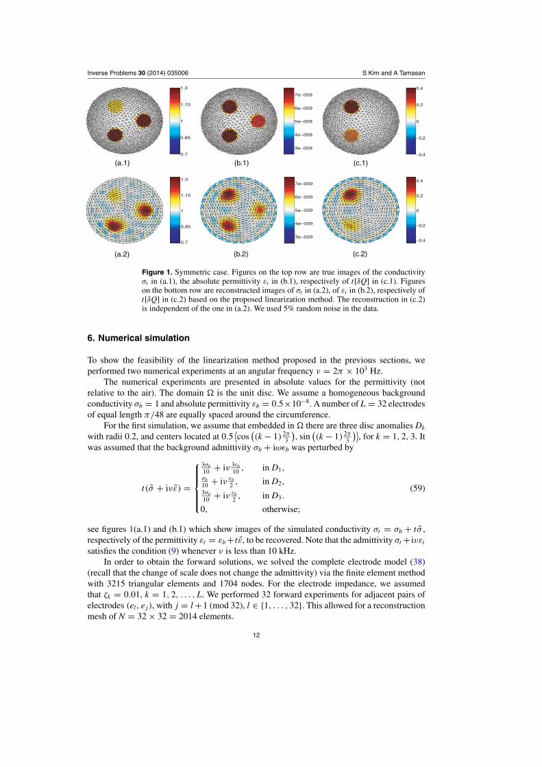
Figure 1. Symmetric case. Figures on the top row are true images of the conductivityσt in (a.1), the absolute permittivity εt in (b.1), respectively of t[δQ] in (c.1). Figureson the bottom row are reconstructed images of σt in (a.2), of εt in (b.2), respectively oft[δQ] in (c.2) based on the proposed linearization method. The reconstruction in (c.2)is independent of the one in (a.2). We used 5% random noise in the data.

6. Numerical simulation

To show the feasibility of the linearization method proposed in the previous sections, weperformed two numerical experiments at an angular frequency ν = 2π × 103 Hz.

The numerical experiments are presented in absolute values for the permittivity (notrelative to the air). The domain � is the unit disc. We assume a homogeneous backgroundconductivity σb = 1 and absolute permittivity εb = 0.5×10−8. A number of L = 32 electrodesof equal length π/48 are equally spaced around the circumference.

For the first simulation, we assume that embedded in � there are three disc anomalies Dk

with radii 0.2, and centers located at 0.5⟨cos

((k − 1) 2π

3

), sin

((k − 1) 2π

3

)⟩, for k = 1, 2, 3. It

was assumed that the background admittivity σb + iωεb was perturbed by

t(σ + iνε) =

⎧⎪⎪⎪⎨⎪⎪⎪⎩

3σb10 + iν 3εb

10 , in D1,σb10 + iν εb

2 , in D2,

3σb10 + iν εb

2 , in D3.

0, otherwise;

(59)

see figures 1(a.1) and (b.1) which show images of the simulated conductivity σt = σb + tσ ,respectively of the permittivity εt = εb + t ε, to be recovered. Note that the admittivity σt + iνεt

satisfies the condition (9) whenever ν is less than 10 kHz.In order to obtain the forward solutions, we solved the complete electrode model (38)

(recall that the change of scale does not change the admittivity) via the finite element methodwith 3215 triangular elements and 1704 nodes. For the electrode impedance, we assumedthat ζk = 0.01, k = 1, 2, . . . , L. We performed 32 forward experiments for adjacent pairs ofelectrodes (el, e j), with j = l +1 (mod 32), l ∈ {1, . . . , 32}. This allowed for a reconstructionmesh of N = 32 × 32 = 2014 elements.

12

Inverse Problems 30 (2014) 035006 S Kim and A Tamasan

To introduce noise in the simulated data Ul jω = (Ul j

ω,1,Ul jω,2, . . . ,Ul j

ω,L) ∈ CL in (40) we

computed the solution ψl jω to (38) at the background admittivity, and let

� l jω =

(∫e1

ψ l jω ds,

∫e2

ψ l jω ds, . . . ,

∫eL

ψ l jω ds

)∈ C

L.

For reconstruction, we added the nos lev = 5% random noise to the forward simulated databy the formulas

�(Ul jω ) + (nos lev) ∗

√[�(Ul j

ω − �l jω

)]2

M∗ (rand num),

(Ul jω ) + (nos lev) ∗

√[ (Ul j

ω − �l jω

)]2

M∗ (rand num),

where rand num is a vector of random numbers distributed in (−1, 1).Using the fdEIT/ data the goal is to reconstruct the quantity

t[δQ] = t

(ε

εb− σ

σb

)=

⎧⎪⎪⎨⎪⎪⎩

0 in D1,

0.4 in D2,

0.2 in D3

0 otherwise

(60)

shown in figure 1(c.1); note that the scaling in permittivity leaves tδQ invariant.In the reconstruction we used the same configuration of electrodes to generate the harmonic

functions φgl j , and φ fα , i.e. α’s were of the type 〈0, . . . , 1,−1, 0, . . .〉. The reconstruction isbased on solving the N × N linear system (52) with N = 32 × 32 = 2014. The sensitivitymatrix in (52) was computed by using the corresponding forward solutions in the absence ofthe anomaly. No regularization was used for inverting the matrix.

Figure 1(c.2) shows the reconstructed image of the t[δQ] by solving the linear system in(52). The interesting part in this reconstruction is that the fdEIT data is blind to the presenceof the anomaly D1, as forecast theoretically.

Next we use the method in section 5 to separately reconstruct conductivity and permittivityby also employing (single frequency) EIT data encoded in the real part of the voltage potential.Figure 1(a.2) shows the reconstruction of conductivity σt = σb + tσ , with tσ obtained viasolving the linear system (57). In combination with the reconstruction of t[δQ] we are alsoable to recover t ε via (58), and thus the permittivity εt = εb + t ε shown in figure 1(b.2).

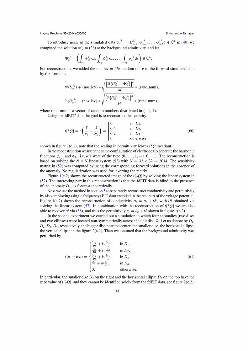
In the second experiment we carried out a simulation in which four anomalies (two discsand two ellipses) were located non-symmetrically across the unit disc �. Let us denote by D1,D2, D3, D4, respectively, the bigger disc near the center, the smaller disc, the horizonal ellipse,the vertical ellipse in the figure 2(a.1). Then we assumed that the background admittivity wasperturbed by

t(σ + iνε) =

⎧⎪⎪⎪⎪⎪⎪⎨⎪⎪⎪⎪⎪⎪⎩

2σb10 + iν 7εb

10 , in D1,

3σb10 + iν 3εb

10 , in D2,

3σb10 + iν 3εb

10 , in D3.σb10 + iν εb

2 , in D4.

0, otherwise.

(61)

In particular, the smaller disc D2 on the right and the horizontal ellipse D3 on the top have thezero value of t[δQ], and they cannot be identified solely from the fdEIT data, see figure 2(c.2).

13

Inverse Problems 30 (2014) 035006 S Kim and A Tamasan

0.7

0.85

1

1.15

1.3

2e−009

3.5e−009

5e−009

6.5e−009

8e−009

−0.4

−0.2

0

0.2

0.4

−0.4

−0.2

0

0.2

0.4

0.8

0.9

1

1.1

1.2

2e−009

3.5e−009

5e−009

6.5e−009

8e−009

(a.1) (b.1) (c.1)

(a.2) (b.2) (c.2)

Figure 2. Non-symmetric case. Figures on the top row are true images of the conductivityσt in (a.1), the absolute permittivity εt in (b.1), respectively of t[δQ] in (c.1). Figureson the bottom row are reconstructed images of σt in (a.2), of εt in (b.2), respectively oft[δQ] in (c.2) based on the proposed linearization method. The reconstruction in (c.2)is independent of the one in (a.2). We used 5% random noise in the data.

7. Conclusions

We present a method to recover small perturbations from constants in the electrical conductivityδσ and relative (to the air’s) permittivity δε of a body from boundary measurements at lowfrequencies.

The method is based on the asymptotic expansion of the frequency differential of theNeumann-to-Dirichlet map with respect to both frequency and perturbation size. Errors dueto neglecting small asymptotic terms are estimated in terms of the coercivity constant, thedomain, and a priori estimates of the perturbations.

From the main asymptotic terms we show that the frequency differential of anappropriately scaled Neumann-to-Dirichlet map recovers δε

εb− δσ

σb. In particular, from frequency

differential data alone, one will not be able to distinguish subregions where the relativeperturbation in conductivity equates the relative perturbation in permittivity. If, in addition,we also take into account the real part of the induced voltage potential, both perturbations δσ

and δε can be determined separately.We propose a numerical scheme based on finitely many electrode configuration, and show

its feasibility in two numerical experiments. In the simulations the domain contains subregionsin which the relative perturbation in conductivity is the same as the relative perturbation inpermittivity. These subregions cannot be distinguished from the background when using thefrequency differential data alone, as explained theoretically. However, when the real part ofthe voltage potential at the boundary is also employed, these subregions are recovered.

Acknowledgments

The authors would like to thank the anonymous referees for their constructive criticism onan earlier version. The first author would like to thank Hanbat National University for the

14

Inverse Problems 30 (2014) 035006 S Kim and A Tamasan

financial support which made his sabbatical visit to A Tamasan at the University of CentralFlorida possible. The work of the second author was supported by NSF grant DMS 1312883.

Appendix. Proof of theorem 2.1

We first establish a basic estimate for the double series of functions satisfying the recurrence(12).

Lemma A.1. Let {v2k} and {h2k−1} be defined recursively in (12). Then[∫�

σ |∇h2k−1|2 dx

] 12

�∥∥∥ ε

σ

∥∥∥2k−1

∞

[∫�

σ |∇v0|2 dx

] 12

, and (A.1)

[∫�

σ |∇v2k|2 dx

] 12

�∥∥∥ ε

σ

∥∥∥2k

∞

[∫�

σ |∇v0|2 dx

] 12

, k = 1, 2, . . . . (A.2)

Proof. Fix an index k. From the divergence theorem we have that∫�

σ |∇h2k−1|2 dx =∫

�

σ∂h2k−1

νh2k−1 ds −

∫�

∇ · (σ∇h2k−1)h2k−1 dx

= (−1)k−1∫

�

( ε

σ

)2k−1gh2k−1 ds +

∫�

∇ · (ε∇v2k−2)h2k−1 dx

= (−1)k−1∫

�

( ε

σ

)2k−1gh2k−1 ds +

∫�

ε∂v2k−2

∂νh2k−1 ds

−∫

�

ε∇v2k−2 · ∇h2k−1 dx

= (−1)k−1∫

�

( ε

σ

)2k−1gh2k−1 ds + (−1)k

∫�

ε

σ

( ε

σ

)2k−2gh2k−1 ds

−∫

�

ε∇v2k−2 · ∇h2k−1 dx = −∫

�

ε∇v2k−2 · ∇h2k−1 dx,

where in the second equality we use the top equation as well as the Neumann boundaryconditions in (12).

By applying Cauchy’s inequality to the right-hand side above we obtain∫�

σ |∇h2k−1|2 dx �∥∥∥ ε

σ

∥∥∥∞

[∫�

σ |∇v2k−2|2 dx

] 12[∫

�

σ |∇h2k−1|2 dx

] 12

,

and thus [∫�

σ |∇h2k−1|2 dx

] 12

�∥∥∥ ε

σ

∥∥∥∞

[∫�

σ |∇v2k−2|2 dx

] 12

. (A.3)

Similarly we obtain[∫�

σ |∇v2k|2 dx

] 12

�∥∥∥ ε

σ

∥∥∥∞

[∫�

σ |∇h2k−1|2 dx

] 12

. (A.4)

By induction, the estimates (A.2) and (A.1) follow. �

15

Inverse Problems 30 (2014) 035006 S Kim and A Tamasan

Proof of theorem 2.1. Upon identifying the real and the imaginary part, The Neumannproblem (1) is equivalent to the following elliptic system:⎧⎪⎪⎪⎪⎪⎪⎨

⎪⎪⎪⎪⎪⎪⎩

∇ · (σ∇vω) = ω∇ · (ε∇hω) in �,

∇ · (σ∇hω) = −ω∇ · (ε∇vω) in �,

−(σ 2 + ω2ε2) ∂vω∂n = σg, on �,

−(σ 2 + ω2ε2) ∂hω∂n = −ωεg, on �,∫

�vω ds = ∫

�hω ds = 0.

(A.5)

�We seek solutions in the ansatz

v(x, ω) :=∞∑

k=0

v2k(x)ω2k, and h(x, ω) :=∞∑

k=1

h2k−1(x)ω2k−1. (A.6)

Let us assume first that the series representation in (A.6) are convergent in H1(�). If(A.5) is satisfied, then

∇ · (σ∇v0) +∞∑

k=1

∇ · (σ∇v2k − ε∇h2k−1)ω2k = 0, and

∞∑k=0

∇ · (σ∇h2k+1 + ε∇v2k)ω2k+1 = 0,

where the divergence is taken in the weak sense. In particular we obtain the top equation in(11) and top two equations in (12).

By our assumption, both series are convergent in H1(�), and therefore ∂vω

∂n , and ∂hω

∂n havewell defined trace in H−1/2(�), which are the corresponding sum of the traces of the terms.Moreover, since the traces of vω and hω are the sum (in H1/2(�)) of the series of the traces ofv2k, and h2k+1, k = 0, 1, . . ., the zero mean condition will be also satisfied for each term v2k,and h2k+1.

We are left to check the Neumann conditions in (12). Starting from the Neumann conditionfor vω in (A.5) we get

(−σ 2 + ω2ε2)

∞∑k=0

∂v2k

∂nω2k = σg.

Upon identifying like terms, it is easy to see that

−σ∂v0

∂n= g, and − σ 2 ∂v2k

∂n= ε2 ∂v2k−2

∂n.

By induction in the second equality above we obtain the Neumann condition for v2k in (12). Asimilar calculation starting from the Neumann condition for hω in (A.5), yields the Neumanncondition for h2k−1 in (12), k = 1, 2, . . ..

Conversely, for g ∈ H−1/2(�) let v0 be the solution of (11) and define two sequences offunctions {vk}∞0 and {hk}∞1 via the recurrence (12). We denote by ‖ · ‖ the L2(�)-norm. From(A.2) it follows that for any k = 1, 2, . . .,

‖∇v2k‖ω2k �√

c

[∫�

σ |∇v2k|2 dx

] 12

ω2k

�√

c∥∥∥ωε

σ

∥∥∥2k

∞

[∫�

σ |∇v0|2 dx

] 12

� c‖∇v0‖∥∥∥ωε

σ

∥∥∥2k

∞, (A.7)

and, similarly,

‖∇h2k−1‖ω2k−1 � c‖∇v0‖∥∥∥ωε

σ

∥∥∥2k−1

∞. (A.8)

16

Inverse Problems 30 (2014) 035006 S Kim and A Tamasan

Now consider the series (A.6) to formally define some v(x, ω) and h(x, ω). We shownext that the series converge in H1(�) and that they satisfy the boundary conditions in (A.5).Indeed, since ω satisfies the frequency range condition

∥∥ωεσ

∥∥∞ < 1, the L2(�)-convergence

of the series of gradients is guaranteed from (A.7) and (A.8) to well define ∇xv(x, ω) and∇xh(x, ω) in L2(�).

Now using the Neumann conditions in (12), and again the frequency range condition (9),we get the H−1/2-summability of the series

∞∑k=0

ω2k ∂v2k

∂ν= − g

σ

∞∑k=0

(−ω2ε2

σ 2

)k

= − σg

σ 2 + ω2ε2. (A.9)

Upon multiplication of (A.9) by arbitrary functions in H1/2(�), integrating over � and applyingGreen’s formula, the duality between H−1/2(�) and H1/2(�) then shows H1/2(�)-summabilityin the series of the traces

∞∑k=0

ω2k v2k|� .

In particular this will carry the zero mean property from each term to the sum.With the L2-summability for the gradient shown previously, we conclude the summability

of the H1(�)-sense. Moreover, the calculation (A.9) showed that

−(σ 2 + ω2ε2)∂v(·, ω)

∂n= σg, on �,

which is the Neumann condition for vω in (A.5).A similar geometric summation as in (A.9), and the duality argument above shows that

the series defining h(·, ω) is also summable in H1(�) and that h(·, ω) satisfies the Neumanncondition for hω in (A.5).

References

[1] Astala K and Paivarinta L 2006 Calderon’s inverse conductivity problem in the plane Ann.Math. 163 265–99

[2] Bayford R H 2006 Bioimpedance tomography (electrical impedance tomography) Annu. Rev.Biomed. Eng. 8 63–91

[3] Beals R and Coifman R R 1985 Multidimensional inverse scatterings and nonlinear partialdifferential equations Pseudodifferential Operators and Applications (Proceedings of Symposiain Pure Mathematics vol 43) (Providence, RI: American Mathematical Society)

[4] Borcea L 2002 Electrical impedance tomography Inverse Problems 18 R99–136[5] Brown B H, Barber D C, Morice A H, Leathard A and Sinton A 1994 Cardiac and respiratory

related electrical impedance changes in the human thorax IEEE Trans. Biomed. Eng. 41 729–34[6] Brown R and Uhlmann G 1997 Uniqueness in the inverse conductivity problem for nonsmooth

conductivities in two dimensions Commun. Partial Differ. Eqns 22 1009–27[7] Bukhgeim A L 2008 Recovering a potential from Cauchy data in the two-dimensional case

J. Inverse Ill-posed Problems 16 19–33[8] Calderon A P 1980 On an inverse boundary value problem Seminar on Numerical Analysis and its

Applications to Continuum Physics ed W H Meyer and M A Raupp (Rio de Janeiro: SociedadeBrasileira de Matematica) pp 65–73

[9] Cheney M, Isaacson D and Newell J C 1999 Electrical impedance tomography SIAMRev. 41 85–101

[10] Francini E 2000 Recovering a complex coefficient in a planar domain from the Dirichlet-to-Neumann map Inverse Problems 16 107

[11] Hamilton S, Herrera C N L, Mueller J and Von Herrmann A 2012 A direct D-bar reconstructionalgorithm for recovering a complex conductivity in 2D Inverse Problems 28 095005

[12] Harrach B and Seo J K 2009 Detecting inclusions in electrical impedance tomography withoutreference measurements SIAM J. Appl. Math. 69 1662–81

17

Inverse Problems 30 (2014) 035006 S Kim and A Tamasan

[13] Harrach B, Seo J K and Woo E J 2010 Factorization method and its physical justification infrequency-difference electrical impedance tomography IEEE Trans. Med. Imaging 29 1918–26

[14] Harrach B and Seo J K 2010 Exact shape-reconstruction by one-step linearization in electricalimpedance tomography SIAM J. Math. Anal. 42 1505–15180

[15] Holder D 2005 Electrical Impedance Tomography: Methods, History and Applications (Bristol:Institute of Physics Publishing)

[16] Kim S, Lee J, Seo J K, Woo E J and Zribi H 2008 Multifrequency trans-admittance scanner:mathematical framework and feasibility SIAM J. Appl. Math. 69 22–36

[17] Kim S, Seo J K and Ha T 2009 A nondestructive evaluation method for concrete voids: frequencydifferential electrical impedance scanning SIAM J. Appl. Math. 69 1759–71

[18] Kim S 2012 Assessment of breast tumor size in electrical impedance scanning InverseProblems 28 025004

[19] Kim S, Lee E J, Woo E J and Seo J K 2012 Asymptotic analysis of the membranestructure to sensitivity of frequency-difference electrical impedance tomography InverseProblems 28 075004

[20] Kim S and Tamasan A 2013 On a Calderon problem in frequency differential electrical impedancetomography SIAM J. Math. Anal. 45 2700–9

[21] Knudsen K 2003 A new direct method for reconstructing isotropic conductivities in the planePhysiol. Meas. 24 391–401

[22] Knudsen K and Tamasan A 2004 Reconstruction of less regular conductivities in the plane Commun.Partial Differ. Eqns 29 361–81

[23] Knudsen K, Lassas M, Mueller J and Siltanen S 2009 Regularized D-bar method for the inverseconductivity problem Inverse Problems Imaging 3 599–624

[24] Knudsen K, Lassas M, Mueller J and Siltanen S 2007 D-bar method for electrical impedancetomography with discontinuous conductivities SIAM J. Appl. Math. 67 893–913

[25] Kohn R V and Vogelius M 1984 Determining conductivity by boundary measurements Commun.Pure Appl. Math. 37 113–23

[26] Nachman A 1988 Reconstructions from boundary measurements Ann. Math. 128 531–76[27] Nachman A 1996 Global uniqueness for a two-dimensional inverse boundary value problem Ann.

Math. 143 71–96[28] Nour S, Mangnall Y F, Dickson J A, Johnson A G and Pearse R G 1995 Applied potential

tomography in the measurement of gastric emptying in infants J. Pediatr. Gastroenterol.Nutr. 20 65–72

[29] Pethig R 1987 Dielectric properties of biological materials Clin. Phys. Physiol. Meas. A 8 5–12[30] Siltanen S, Mueller J and Isaacson D 2000 An implementation of the reconstruction algorithm of

A Nachman for the 2D inverse conductivity problem Inverse Problems 16 681–99[31] Scholz B and Anderson R 2000 On electrical impedance scanning: principles and simulations

Electromedica 68 35–44[32] Schwan H P and Kay C F 1957 The conductivity of living tissue Ann. New York Acad.

Sci. 65 1007–13[33] Seo J K, Lee J, Kim S W, Zribi H and Woo E J 2008 Frequency-difference electrical impedance

tomography (fdEIT): algorithm development and feasibility study Physiol. Meas. 29 929–44[34] Seo J K, Harrach B and Woo E J 2009 Recent progress on frequency difference electrical impedance

tomography ESAIM Proc. 26 150–61[35] Somersalo E, Cheney M and Isaacson D 1992 Existence and uniqueness for electrode models for

electric current computed tomography SIAM J. Appl. Math. 52 1023–40[36] Stojadinovic A et al 2005 Electrical impedance scanning for the early detection of breast

cancer in young women: preliminary results of a multicenter prospective clinical trial J. Clin.Oncol. 23 2703–15

[37] Sylvester J and Uhlmann G 1987 A global uniqueness theorem for an inverse boundary valueproblem Ann. Math. 125 153–69

[38] Tidswell T, Gibson A, Bayford R H and Holder D S 2001 Three-dimensional electrical impedancetomography of human brain activity NeuroImage 13 283–94

[39] Uhlmann G 2009 Electrical impedance tomography and Calderon’s problem InverseProblems 25 1–39

18