IEEE GEOSCIENCE AND REMOTE SENSING LETTERS, VOL. 6, NO. 4, OCTOBER 2009 671

Reconstruction of One-Dimensional DielectricScatterers Using Differential Evolution and

Particle Swarm OptimizationAbbas Semnani, Student Member, IEEE, Manoochehr Kamyab, and Ioannis T. Rekanos, Member, IEEE

Abstract—A comparison between differential evolution (DE)and particle swarm optimization (PSO) in solving 1-D small-scaleinverse scattering problems is presented. In this comparison, theefficiency of both aforementioned optimization techniques is ex-amined for permittivity and conductivity profile reconstructionproblems. The comparison is carried out under the same con-ditions of initial population of candidate solutions and numberof iterations. Numerical results indicate that both optimizationmethods are reliable tools for inverse scattering applications evenwhen noisy measurements are considered. In the particular caseof small-scale problems investigated in this letter, DE outperformsthe PSO in terms of reconstruction accuracy. This is considered anindicative result and not generally applicable.

Index Terms—Differential evolution (DE), inverse scattering,particle swarm optimization (PSO), profile reconstruction.

I. INTRODUCTION

THE reconstruction of the electromagnetic properties of1-D scatterers from scattered field measurements belongs

to the general class of inverse scattering problems and is intrin-sically a nonlinear and ill-posed problem [1]. Usually, the scat-terer is reconstructed by updating iteratively the profile of theunknown scatter properties, while the whole approach is basedon the minimization of the discrepancy between measuredand estimated field data. Two basic approaches are followedto solve the inverse scattering problem, namely, the use oflocal and global search algorithms. Local search is achievedby means of gradient-based optimization algorithms that arecomputationally fast but are usually trapped into local minima[2], [3]. The global search algorithms, which are stochasticor evolutionary, can avoid being trapped in local minima butrequire significant computation time to converge (see [4] andreferences within).

Since their initial development, evolutionary optimizationalgorithms have been applied successfully in the solution ofelectromagnetic inverse scattering problems. These applica-tions can be categorized into two groups with respect to thenumber of the unknown parameters that describe the scattererproperties or equivalently the size of the scatterer. In the first

Manuscript received November 13, 2008; revised April 7, 2009. First pub-lished June 23, 2009; current version published October 14, 2009. This workwas supported by the Iran Telecommunication Research Center under GrantT-500-19708.

A. Semnani and M. Kamyab are with the Department of Electrical Engineer-ing, K. N. Toosi University of Technology, Tehran 14317-14191, Iran (e-mail:a_semnani@eetd.kntu.ac.ir; kamyab@eetd.kntu.ac.ir).

I. T. Rekanos is with the Physics Division, School of Engineering,Aristotle University of Thessaloniki, 54124 Thessaloniki, Greece (e-mail:rekanos@auth.gr).

Digital Object Identifier 10.1109/LGRS.2009.2023246

category, namely, the small-scale inverse scattering applica-tions, the number of unknown parameters is small [5]–[9],whereas in the second category (large-scale applications) thesize of the scatterers and consequently the number of unknownsare large [10], [11]. Among the evolutionary optimization tech-niques, the differential evolution (DE) algorithm [12] and theparticle swarm optimization (PSO) [13] are relatively recentones. The DE has been applied in the shape reconstruction ofconducting scatterers [9], [14], [15] and the reconstruction ofburied dielectric objects [8], whereas the PSO has been utilizedin the reconstruction of dielectric scatterers [7], [16], [17]. Thereported results indicate that both DE and PSO are reliabletools and outperform real-coded genetic algorithms in terms ofconvergence speed [15], [16]. Moreover, a comparative studyabout the performance of these two techniques, when appliedto the shape reconstruction of perfectly conducting scatterers,has recently been reported [9], where DE outperformed PSO.Although this result was indicative [9], it could not lead tothe general conclusion that DE outperforms PSO in all inversescattering problems. Hence, further comparisons are needed,particularly when dielectric scatterers are considered.

In this letter, we compare the performance of DE and PSOwhen applied to profile reconstruction of either lossless orlossy dielectric scatterers. In particular, we consider a small-scale applications because the scatterers are considered 1-D.A brief overview on DE and PSO is presented in Section II.In Section III, the reconstruction of inhomogeneous losslessor lossy scatterers is considered, while the efficiency of bothmethods is examined. Finally, some brief conclusions follow inSection IV.

II. BRIEF OVERVIEW ON DE AND PSO

Let us assume that the objective is to minimize a costfunction F (x) with respect to the vector of parameters,x = [x1, x2, . . . , xN ], where N is the dimension of the so-lution space. Evolutionary optimization algorithms are basedon a population of candidate solutions xk, k = 1, 2, . . . ,K,(K is the population size), that are updated iteratively searchingthe solution space for the global minimum of F (x).

In DE, after generating the initial population, the candidatesolutions are refined by applying mutation, crossover and selec-tion, iteratively. During mutation, for each individual solutionxk, three distinct solutions, xr1, xr2, and xr3, which aremutually different and different from xk, are randomly selectedto generate a new solution, yk, i.e.,

yk = xr1 + β(xr2 − xr3) (1)

1545-598X/$26.00 © 2009 IEEE

672 IEEE GEOSCIENCE AND REMOTE SENSING LETTERS, VOL. 6, NO. 4, OCTOBER 2009

Fig. 1. Geometrical configuration of the problem.

where β is the mutation factor. Then, crossover results in thegeneration of the final offspring uk, according to the scheme

ukn ={

ykn, if hn ≤ Hxkn, if hn > H

(2)

n = 1, 2, . . . , N , hn is a random number uniformly distributedwithin [0, 1] and H ∈ (0, 1) is a predefined crossover probabil-ity. It should be mentioned that uk has to inherit at least onecomponent from yk. Finally, during selection, the offspring,uk, competes with the initial solution candidate, xk, and if itis fittest with respect to the cost function, it replaces xk in thenext generation, i.e.,

xk ←{

uk, if F (uk) ≤ F (xk)xk, if F (uk) > F (xk). (3)

In PSO, each candidate solution xk is considered as a particleand has a velocity, vk, used to move around the solution space.In particular, the new position of the particle is given by

xk ← xk + vk (4)

while the components of the velocity vector are updated accord-ing to the scheme

vkn←w · vkn+c1 · q1 ·(xb

kn−xkn

)+c2 · q2 · (gn−xkn). (5)

In (5), w in the inertia, c1 is the cognitive, and c2 the socialparameter, whereas q1 and q2 are random numbers uniformlydistributed in [0, 1]. In addition, xb

k = [xbk1, x

bk2, . . . , x

bkN ] is

the best position ever visited by the kth particle, while g =[g1, g2, . . . , gN ] is the global best position found by the wholepopulation. Obviously, if the new particle position derived from(4) is fittest than xb

k, then the latter is updated. Furthermore, gis updated respectively.

III. NUMERICAL RESULTS

We consider the case of an 1-D inhomogeneous scatterer(Fig. 1), which can be either lossless or lossy. The scatterer isinfinite in the plane perpendicular to x-axis and it is boundedwithin the area 0 ≤ x ≤ a. The relative permittivity εr and theconductivity σ of the scatterer depend only on x, whereas thesurrounding medium is considered to be free space.

The scatterer is illuminated by a plane wave propagatingalong the positive x-direction, while the electric field has the

form of Gaussian pulse in time. The total electric field ismeasured at two distinct measurement points placed at eachside of the scatterer. The solution of the direct scatteringproblem is carried out by means of the FDTD method appliedto the discretized x-axis. In the FDTD code, the excitationfield is set at a point as shown schematically in Fig. 1. Thescatterer region is discretized into M equal line segmentswhere within each segment the scatterer properties (relativepermittivity and conductivity) are considered constant. Thus,if the scatterer is lossy, its profile is described by the vectorx = [εr1, σ1, εr2, σ2, . . . , εrM , σM ], whereas if the scattereris lossless, then x = [εr1, εr2, . . . , εrM ]. The objective of theinverse scattering procedure is the estimate x by minimizingthe cost function

F (x) =

∑i=1,2

∑Tt=1 |Ee

it(x) − Emit |

2∑i=1,2

∑Tt=1 (Em

it )2+ λR(x) (6)

where Ee and Em are the estimated and the measured field,respectively, while i denotes the measurement point and t is thetime index. In (6), R(x) is the total variation regularization term[18] introduced to cope with the ill-posedness, while λ is theregularization factor. In all the following numerical examples,the regularization factor is λ = 0.001, and the cost functionis identical for both DE and PSO to derive fair comparativeresults. To quantify the reconstruction accuracy of DE and PSO,the reconstruction errors of relative permittivity and conductiv-ity are defined as

e(ε) = 100 ·√∑M

m=1 |εrm − εorm|2∑M

m=1 (εorm)2

(7)

e(σ) = 100 ·√∑M

m=1 |σm − σom|2∑M

m=1 (σom)2

(8)

respectively, where “o” denotes the original scatterer properties.Two reconstruction test cases are investigated. First, we

consider a lossless dielectric scatterer, which is discretized intoM = 30 segments. Hence, the dimension of the solution spaceis N = M = 30. Two different population sizes, i.e., K = 30and K = 60, have been considered for both DE and PSO,while the total number of iterations is set equal to 500. Therelative permittivity values in the initial population are selectedrandomly (uniformly distributed in the range [1, 5]). Both DEand PSO are applied to 30 different initial populations, whilefor each initial population ten executions have been performed.Hence, 300 runs for each population size and both DE and PSOhave been executed, while the mean value and the standarddeviation of the cost function and the reconstruction errorare evaluated. It is mentioned that each initial population isconsidered identical for both DE and PSO applications.

Concerning the DE implementation, the mutation factor isβ = 0.5, whereas the crossover probability is H = 0.8. In thePSO, the inertia parameter w is initially equal to 1.0 anddrops linearly to 0.7 after 500 iterations. The cognitive andsocial parameters are c1 = c2 = 0.5. The selection of the aboveparameter values in the implementation of DE and PSO is basedon a parametric study and results in the best performance ofboth methods. It is noted that the above values are similarto those adopted in [9]. The numerical results related to the

SEMNANI et al.: RECONSTRUCTION OF 1-D DIELECTRIC SCATTERERS 673

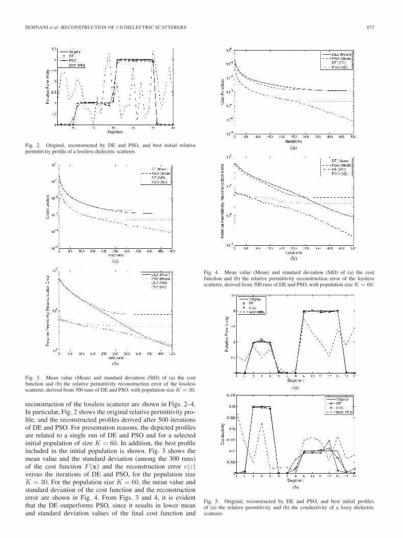
Fig. 2. Original, reconstructed by DE and PSO, and best initial relativepermittivity profile of a lossless dielectric scatterer.

Fig. 3. Mean value (Mean) and standard deviation (StD) of (a) the costfunction and (b) the relative permittivity reconstruction error of the losslessscatterer, derived from 300 runs of DE and PSO, with population size K = 30.

reconstruction of the lossless scatterer are shown in Figs. 2–4.In particular, Fig. 2 shows the original relative permittivity pro-file, and the reconstructed profiles derived after 500 iterationsof DE and PSO. For presentation reasons, the depicted profilesare related to a single run of DE and PSO and for a selectedinitial population of size K = 60. In addition, the best profileincluded in the initial population is shown. Fig. 3 shows themean value and the standard deviation (among the 300 runs)of the cost function F (x) and the reconstruction error e(ε)versus the iterations of DE and PSO, for the population sizeK = 30. For the population size K = 60, the mean value andstandard deviation of the cost function and the reconstructionerror are shown in Fig. 4. From Figs. 3 and 4, it is evidentthat the DE outperforms PSO, since it results in lower meanand standard deviation values of the final cost function and

Fig. 4. Mean value (Mean) and standard deviation (StD) of (a) the costfunction and (b) the relative permittivity reconstruction error of the losslessscatterer, derived from 300 runs of DE and PSO, with population size K = 60.

Fig. 5. Original, reconstructed by DE and PSO, and best initial profilesof (a) the relative permittivity and (b) the conductivity of a lossy dielectricscatterer.

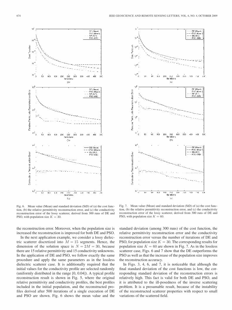
674 IEEE GEOSCIENCE AND REMOTE SENSING LETTERS, VOL. 6, NO. 4, OCTOBER 2009

Fig. 6. Mean value (Mean) and standard deviation (StD) of (a) the cost func-tion, (b) the relative permittivity reconstruction error, and (c) the conductivityreconstruction error of the lossy scatterer, derived from 300 runs of DE andPSO, with population size K = 30.

the reconstruction error. Moreover, when the population size isincreased the reconstruction is improved for both DE and PSO.

In the next application example, we consider a lossy dielec-tric scatterer discretized into M = 15 segments. Hence, thedimension of the solution space is N = 2M = 30, becausethere are 15 relative permittivity and 15 conductivity unknowns.In the application of DE and PSO, we follow exactly the sameprocedure and apply the same parameters as in the losslessdielectric scatterer case. It is additionally required that theinitial values for the conductivity profile are selected randomly(uniformly distributed in the range [0, 0.04]). A typical profilereconstruction result is shown in Fig. 5, where the originalrelative permittivity and conductivity profiles, the best profilesincluded in the initial population, and the reconstructed pro-files derived after 500 iterations of a single execution of DEand PSO are shown. Fig. 6 shows the mean value and the

Fig. 7. Mean value (Mean) and standard deviation (StD) of (a) the cost func-tion, (b) the relative permittivity reconstruction error, and (c) the conductivityreconstruction error of the lossy scatterer, derived from 300 runs of DE andPSO, with population size K = 60.

standard deviation (among 300 runs) of the cost function, therelative permittivity reconstruction error and the conductivityreconstruction error versus the number of iterations of DE andPSO, for population size K = 30. The corresponding results forpopulation size K = 60 are shown in Fig. 7. As in the losslessscatterer case, Figs. 6 and 7 show that the DE outperforms thePSO as well as that the increase of the population size improvesthe reconstruction accuracy.

In Figs. 3, 4, 6, and 7, it is noticeable that although thefinal standard deviation of the cost functions is low, the cor-responding standard deviation of the reconstruction errors isrelatively high. This fact is valid for both DE and PSO, andit is attributed to the ill-posedness of the inverse scatteringproblem. It is a presumable result, because of the instabilityof the reconstructed scatterer properties with respect to smallvariations of the scattered field.

SEMNANI et al.: RECONSTRUCTION OF 1-D DIELECTRIC SCATTERERS 675

TABLE ILOSSLESS SCATTERER CASE—COST FUNCTION F (x) AND

RECONSTRUCTION ERROR e(ε) AFTER 500 ITERATIONS OF DE AND

PSO FOR VARIOUS SNR LEVELS OF THE MEASUREMENTS

TABLE IILOSSY SCATTERER CASE—COST FUNCTION F (x) AND

RECONSTRUCTION ERRORS e(ε) AND e(σ) AFTER 500 ITERATIONS OF

DE AND PSO FOR VARIOUS SNR LEVELS OF THE MEASUREMENTS

The performance of the DE and PSO in case of noisy electricfield measurements has also been examined. The measurementshave been corrupted by additive white Gaussian noise withdifferent signal-to-noise ratio (SNR). A single initial populationof size K = 60 has been considered in all reconstruction at-tempts. For the case of the lossless scatterer studied previously,the cost function and the reconstruction error derived after 500iterations of DE and PSO, when applied to measurements ofdifferent SNR levels, are shown in Table I. The correspondingresults for the lossy scatterer are presented in Table II. Fromboth Tables I and II, we conclude that even in case of noisymeasurements, DE outperforms PSO basically with respectto the final reconstruction error, resulting in more accuratereconstruction.

Finally, the computation time for both DE and PSO is almostidentical, because the population size and the number of itera-tions are considered to be the same. The computational burdenis basically governed by the time required for solving the directscattering problem, iteratively.

IV. CONCLUSION

The small-scale problem of profile reconstruction of 1-Ddielectric scatterers (both lossless and lossy) has been investi-gated by applying the DE and the PSO optimization techniques.Numerical results show that both methods result in accuratereconstruction even when noisy measurements are considered.Although PSO shows slightly better convergence rate at the

initial iterations, finally, DE leads to more precise reconstruc-tion results for the same population size and total number ofiterations. It should be mentioned that this comparative study isindicative and its conclusion should not be considered generallyapplicable in all inverse scattering problems.

REFERENCES

[1] A. N. Tikhonov and V. Y. Arsenin, Solutions of Ill-Posed Problems.Washington, DC: Winston, 1977.

[2] A. Abubakar and P. M. van den Berg, “Iterative forward and inverse algo-rithms based on domain integral equations for three-dimensional electricand magnetic objects,” J. Comput. Phys., vol. 195, no. 1, pp. 236–262,Mar. 2004.

[3] I. T. Rekanos, T. V. Yioultsis, and C. S. Hilas, “An inverse scatteringapproach based on the differential E-formulation,” IEEE Trans. Geosci.Remote Sens., vol. 42, no. 7, pp. 1456–1461, Jul. 2004.

[4] M. Pastorino, “Stochastic optimization methods applied to microwaveimaging: A review,” IEEE Trans. Antennas Propag., vol. 55, no. 3,pp. 538–548, Mar. 2007.

[5] A. Qing, “Dynamic differential evolution strategy and applicationsin electromagnetic inverse scattering problems,” IEEE Trans. Geosci.Remote Sens., vol. 44, no. 1, pp. 116–125, Jan. 2006.

[6] S. Caorsi, A. Massa, M. Pastorino, and A. Randazzo, “Electromagneticdetection of dielectric scatterers using phaseless synthetic and real dataand the memetic algorithm,” IEEE Trans. Geosci. Remote Sens., vol. 41,no. 12, pp. 2745–2753, Dec. 2003.

[7] T. Huang and A. S. Mohan, “A microparticle swarm optimizer for thereconstruction of microwave images,” IEEE Trans. Antennas Propag.,vol. 55, no. 3, pp. 568–576, Mar. 2007.

[8] A. Massa, M. Pastorino, and A. Randazzo, “Reconstruction of two-dimensional buried objects by a differential evolution method,” Inv.Probl., vol. 20, no. 6, pp. S135–S150, Dec. 2004.

[9] I. T. Rekanos, “Shape reconstruction of a perfectly conducting scat-terer using differential evolution and particle swarm optimization,” IEEETrans. Geosci. Remote Sens., vol. 46, no. 7, pp. 1967–1974, Jul. 2008.

[10] M. Donelli and A. Massa, “Computational approach based on a particleswarm optimizer for microwave imaging of two-dimensional dielectricscatterers,” IEEE Trans. Microw. Theory Tech., vol. 53, no. 5, pp. 1761–1776, May 2005.

[11] G. Franceschini, D. Franceschini, and A. Massa, “Full-vectorial three-dimensional microwave imaging through the iterative multiscalingstrategy—A preliminary assessment,” IEEE Geosci. Remote Sens. Lett.,vol. 2, no. 4, pp. 428–432, Oct. 2005.

[12] R. Storn and K. Price, “Differential evolution—A simple and efficientheuristic for global optimization over continuous space,” J. Glob. Optim.,vol. 11, no. 4, pp. 341–359, Dec. 1997.

[13] J. Kennedy and R. C. Eberhart, “Particle swarm optimization,” in Proc.IEEE Conf. Neural Netw., 1995, vol. 4, pp. 1942–1948.

[14] K. A. Michalski, “Electromagnetic imaging of circular-cylindrical con-ductors and tunnels using a differential evolution algorithm,” Microw. Opt.Technol. Lett., vol. 27, no. 5, pp. 330–334, Dec. 2000.

[15] A. Qing, “Electromagnetic inverse scattering of multiple two-dimensionalperfectly conducting objects by the differential evolution strategy,” IEEETrans. Antennas Propag., vol. 51, no. 6, pp. 1251–1262, Jun. 2003.

[16] M. Donelli, G. Franceschini, A. Martini, and A. Massa, “An integratedmultiscaling strategy based on a particle swarm algorithm for inversescattering problems,” IEEE Trans. Geosci. Remote Sens., vol. 44, no. 2,pp. 298–312, Feb. 2006.

[17] A. Semnani and M. Kamyab, “Truncated cosine Fourier series expansionmethod for solving 2-D inverse scattering problems,” Prog. Electromagn.Res. (PIER), vol. 81, pp. 73–97, 2008.

[18] A. Abubakar and P. M. van den Berg, “Total variation as a multiplicativeconstraint for solving inverse problems,” IEEE Trans. Image Process.,vol. 10, no. 9, pp. 1384–1392, Sep. 2001.