1

Rectilinear Motion

A Basis for the Adaptation of Arbitrary Motions

E. F. M. Jochim

German Aerospace Centre, Oberpfaffenhofen, Germany

Tel: (-)49-(0) 8153-28-2738, Fax: (-)49-(0)-8153-28-1452, e-mail: Fritz.Jochim@dlr.de

Summary: Rectilinear motion will be used for the adaptation of any motion based on the method of the variation of the parameters. The formulae will be derived with respect to Han-sen’s “Ideal” coordinates. Examples show the use of the method. Based on rectilinear motion, a generalization of Kepler’s distance law is established which is valid for any motion.

Keywords: Rectilinear motion, adaptation of any motion, variation of parameters, Lagrange constraint, Keplerian distance law, general distance law, Hansen (“Ideal”) frame, Leibniz frame

Table of Symbols:

AR equal area for solar radiation [m2]

AU astronomical unit ( 81.49597870 10 [km])

bR, bT, bN accelerations in radial, transversal, normal directions [km/s2]

bR2 radial “perturbation” of a 2-body motion [km/s2]

bRC constant radial acceleration [km/s2]

bRK Keplerian acceleration [km/s2]

bSR radial acceleration due to thruster impuls [km/s2]

c1, c2, C1, C2 integration constants of rectilinear motion (vector, scalar resp.)

cR reflectivity coefficient

d distance along curve for equal area law [km]

e numerical eccentricity of conic section

G equal area parameter [km2/s]

g auxiliary factor g=s/V [sec]

g1, g2 parameter vector components, 1 2cos , sinP Pg V g V [km/s]

2

ip Basis vectors of inertial system (Newton frame)

PS Solar pressure [kg/(ms2)]

p semilatus rectum of conic section [km]

0 0 0, ,r q c Basis vectors of co-moving system (orbit system, Leibniz frame)

r, rP radius, radius of pericentre distance [km]

rK radius of a circular orbit [km] ( )Ijq Basis vectors of Ideal system (Hansen frame)

s Distance along curve [km]

t, tP time, time of pericentre passage [s]

V velocity [km/s]

orbit angle (first Hansen angle) [rad]

P orbit angle (Hansen angle) [rad] of pericentre

spatial rotation angle (second Hansen angle) [rad]

centric gravitational constant [km3/s2]

M heliocentric gravitational constant ( 20 3 21.32712438 10 /m s M )

1 The Idea of Rectilinear Motion

Xenophanes of Kolophon (, ca. 570 - 475 B.C.) seems to be the first, and proba-bly the only, of the Pre-Socratian philosophers to assume a rectilinear motion of the celestial bodies

"Xenophanes ...says, the Sun would move to the infinite, however, due to the great distance its motion would appear to be circular" )1.

He assumed that the Sun, the Moon and the stars were glowing clouds. They will be newly produced every day in the morning and they will cease glowing in the evening. All other Pre-Socratian philosophers seemed to believe in circular motion of the celestial bodies, an idea going back to Anaximander of Miletus.

Aristotle 384 - 322 B.C.) assumes three basic motions: a rectilinear motion towards the centre of the Earth, a rectilinear motion away from the centre of the Earth, and a circular motion. All other motions will be composed of these kinds of motion:

1 [1] fr. R 13, [2] DK 21A41a

3

(„Because each motion in space, we call it to carry, will be rectilinear or circular or mixed of both of them. Because these two are the only simple motions“)2.

Aristotle again justifies this statement:

(„The reason is why only these two parameters are simple, the rectilinear and what is moved in a circle“)3.

Aristotle believes the circular motion to be the primary of all motions, in contrast to rectiline-ar motion:

In addition, such a motion will necessarily be the first. The reason for this is that it is natural that the perfect will be earlier than the imperfect. The circle is part of perfect things, but the rectilinear line will never be perfect. “)4.

By way of these statements, Aristotle became responsible for thousands of years preference for circular motion.

In a mathematical sense, Proclus (412 - 485 A.D.) linked circular and rectilinear motion by the so-called Proclus device (cf. Figure 1), which was later (in the 13th century) applied by Nasir ad Din at T usi

as “Tusi’s device”, in order to improve the theory of planetary

latitudes originated by Ptolemy. 4

-NOV

-97 14

:57:1

2

U

U

U U

U

U

L

K

F

H AD

r

rr

Figure 1: The Theorem of Proclus („Proclus’ device“): When H moves on the line DA towards the centre D and K is moving in the same time on the line DL towards L, then F, which is in the middle of the line HK, is moving

on a circle centred on D

In a philosophical sense, Nikolaus of Kues (known as Cusanus, 1401-1464, A.D.) linked circular and rectilinear motion by his method of “Coincidentia Oppositorum” (= the coinci-dence of opposite extremes). As an example, he used a circle with infinite radius, which will be a rectilinear line.

2 [3] de caelo A II, 268b17 3 [3] de caelo A II, 268b19 4 [3] de caelo A II, 269 a 19-21

4

In a mathematical sense, this idea of Cusanus was reflected in the theory of rotations devel-oped by Benjamin Olinde Rodrigues (1795–1850). In his theory, the Eulerian division of any motion into a rotational and a translatorial part is replaced by two consecutive rotations: instead of the translation, Rodrigues assumes a rotation with respect to a central axis in infi-nite distance, and perpendicular to the direction of motion5.

A physical interpretation of the rectilinear motion was given by Galileo Galilei (1564-1642) by his detection of the law of inertia:

„A body is moving uniformly and rectilinearly if there is no force acting on it“.

In his publication Dialog, there is the following citation of the motion of a body catapulted around and then released6:

1. „The motion impressed on the body, free flying after separation, can only be a rectilinear motion“

2. „A thrown body moves along the tangent of the circle at the point of separation“.

3. „Immediately after separation, the thrown body will have another direction of motion as the thrown body had before separation“.

Figure 2: Galileo’s drawing describing the motion of a throw (copy from Galileo’s dialog7)

In contrast to planetary motion, Johannes Kepler (1751 – 1630) assumed a nearly rectilinear motion for the comets8. However, implicit in his second law, the cross-product of the position and velocity vector permits the adaptation of motion at the position described by the position vector by a rectilinear motion along the tangent in direction of the velocity vector.

It can be shown that no circle is able to be adapted to any motion9. In the following sections, however, it will be shown that a straight line can be adapted to any motion.

5 [14], p. 375 6 see [4], p.120 7 copy from [4], p.120 8 see [10], p.288 9 see [5]

5

2 A Mathematical Description of Rectilinear Motion

2.1 The Basic Equations

Based on the law of inertia, uniform rectilinear motion will be possible if there are no pertur-bations acting on the moving body. Therefore from

0r (1)

two integrations with respect to time t in an inertial space frame lead to the position vector

1 2 .t r c c (2)

In this solution, the first constant is identical to the velocity vector

1 ,c r (3)

the second constant vector c2 marks an initial position along the orbit.

Relating to a co-moving rectangular coordinate system with direction vectors r0 in the radial, q0 in the transversal (“transradial”), and c0 in the normal direction, the acceleration vector describing the motion can be written in the form

0 0 0 .R T Nb b b r r q c (4)

According to the accompanying trihedron10, r0, q0, c0, the acceleration is divided in the radial bR, the transversal bT and the normal bN acceleration. If r is the radius of the moving body and

0rr r (5)

is the position vector, then the velocity vector is given by

0 0 0 0 .r r r r r r r r q (6)

If, and only if, 0: r is assumed to be the value of the variation of the radial direction vec-

tor r0, then can be shown to be an orbit angle related to the motion oriented Hansen (“Ide-al”) coordinate system11. (A Hansen system is a coordinate system in which the velocity vec-tor is independent of the proper motion of this system). This leads to the orbit normal vector12

2 20 0 0, 1, 0 ,r G G c r r c c c c (7)

where the general relation 2r G is completely independent of any orbit form. Because

0G , this relation includes the following issue: if the parameter is interpreted as usual as an orbit angle, its direction of variation must always be positive13. The equation (7) corre-sponds to the second Keplerian law if, and only if, the equal area parameter G[km2/s] is a

10 As firstly introduced into celestial mechanics by G.W. Leibniz [7], therefore, this system is sometimes called “Leibniz frame” 11 see [6], theorem 13, advice also in [19], p.69 12 the value of the orbit normal vector will be designed with the symbol G according to the corresponding ca-nonical element in Ch. Delaunay’s theory and is in this form already widely used in Astrodynamics 13 cf. e.g. [17], p. 46

6

constant. The acceleration related to the co-moving coordinate system (“orbit system”, “Leib-niz frame”) is

0 0 0 02 .r r r r r r q q q (8)

Introducing parameters , and because 20 1q , the variation of the transversal direction

vector q0 can only take place in a plane perpendicular to this vector

0 0 0: . q r c (9)

The motion acceleration vector is then

0 0 02 .r r r r r r r q c (10)

Therefore, by comparing equations (4) and (10), and applying (7), the transversal acceleration leads to the variational equation for the parameter G based on the transversal acceleration only

.TG r b (11)

The variational equation for the parameter is based on the normal acceleration only

.N

rb

G (12)

It can be shown14 that is a consequence of the relation to a Hansen system, therefore, the general equation of motion can be written in the form

2

0 0 03.

G G Gr

r r r

r r q c

(13)

Comparison with equation (4) finally leads to the “general Leibniz equation”

2

3.R

Gr b

r (14)

In case of the two body problem, G. W. Leibniz15 derived this equation based on the Keplerian acceleration bR -1/r2 and taking into account the first two Keplerian laws16.

If no acceleration acts on the motion, then bR = bT = bN = 0 and G = const. and = const. (= 0). In this case, the Leibniz equation leads to the first integral

2

21 2

.G

r Cr

(15)

The new constant C1[km/s] has to fulfil the condition

1

0G

rC

. (16)

14 see [6] section 4, formula (57) and theorem 15 15 see [7] 16 cf. [8], p. 67

7

Following equation (7), G is non-negative and 1C must be positive. Therefore the auxiliary

parameter

2 2 21:g r C G (17)

can be used. A geometrical interpretation of this parameter is possible according to Figure 3:

1/g C is the (arc-) length along the (rectilinear) orbit as counted from the orbit point next to

the initial point P (the „pericentre“ of the rectilinear orbit) and the position r of the orbit. Be-cause

21 ,gg C r r (18)

and, using the differential equation (15), it follows that

2 2 21 ,r r r C G g (19)

therefore,

21 .g C (20)

This leads to the integral

21 2g C t C . (21)

C2[km2/s] is the new integrational constant. The radius will be calculated from equation (17):

2 2

2 2 21 2 2

1

2 .C G

r C t C tC

(22)

S

M

P

r

C1

g

GC1

Figure 3: Diagram of the rectilinear motion

In orbital mechanics, the orbit angle usually replaces the time t by means of equation (7)

2 22

2 2 21 2 2

1

2

G G dtd dt

C GrC t C t

C

(23)

with the integral

21 2

1arctanP C t C

G

or

8

2 11 2

1

1tan( ) .P

ss C

C t CGG GC

(24)

Applying equation (17), we have

2 2 21

1tan( ) .P C r G

G (25)

The new integrational constant P can be related to C2 by

2tan ( 0) , : ( ) .P P P

Ct t t

G (26)

This relation is geometrically interpreted in Figure 4.

S(t=0)

M

P

r(t=0) GC1

C1

C2

O

(t=0)

q1(I)

P

Figure 4: The relation of the parameter P and C2 of the rectilinear motion

According to equation (24), the time t and orbit angle are connected. The time can be de-rived from the orbit angle via

221

1tan( )Pt G C

C . (27)

Because C1 > 0, this relationship has no singularity. In order to relate the constant C2 to the initial time tP, we define the pericentre distance at the moment of the pericentre pass as

1

: ( )P P

Gr r t

C . (28)

Using equation (21) we have

22 1 .PC C t (29)

From equation (25), the expression for the radius with respect to the orbit angle will be

1

.cos( )P

Gr

C

(30)

9

S

M

P

rGC1

O

C1

gs=

r

r

1(I)q

Figure 5: Rectilinear motion: The geometrical visualization of the mathematical description

This relation has no singularity since, with 0G and 1 0C , it is always the case that

cos( ) 0P and the angle P must lie in the interval

90 90P . (31)

Figure 5 confirms that the singularity 90P will never happen, whenever the origin

M is not lying on the straight line of the rectinlinear motion.

The variation of the radius (i.e. the radial velocity) will follow from equation (15)

1 sin( ) .R PV r C (32)

Based on equations (19), (21), (22) and (29), the following relation can be derived

2 21 2 1tan( ) ( ) .P Pr r G C t C C t t (33)

Finally, the transversal velocity will be found using equation (7), and taking into account equation (30):

1 cos .T P

GV r C

r (34)

With the radial and the transversal velocities derived in equations (32) and (34), the velocity vector (6) leads to

1 0 0sin( ) cos( ) .P PC r r q

If the absolute velocity is assumed to be V r then

2 2 21 ,V C r (35)

and because C1>0, it is shown that the first constant of the rectilinear motion is identical to the velocity

1 .C V (36)

In conclusion, the state vector of the rectilinear motion is

10

0 0 0, sin cos( ) ,

cos P PP

GV

V

r r r r q (37)

the radius, radial, and transversal velocity are given by

cos

sin

cos

P

R P

T P

Gr

V

V r V

V r V

(38)

and we find

2 ( ) tan .P Pr r V t t G (39)

2.2 The Law of Areas in Rectilinear Motion

Kepler’s second law is a general behaviour of any central motion as shown by L. Euler17. This law has no other content than to state that the behaviour of such a motion always takes place in a fixed plane. This will be represented by

, const. r r c c

We would like to investigate the area law in case of a (uniform) rectilinear motion. In this case of constant velocity, .V const , the body will always travel in equal time intervals, t , the same distance

.d V t (40)

U

U

M

U

rU

rP

rU

r

Udd

F

CD

FP

P-

S

Figure 6: The area law for the case of uniform rectilinear motion

According to Figure 6, the area FP formed by the triangle MPSP should be the pericentre in relation to a fictive origin M) shall be set in relation to the area F of a triangle MCD at any

17 published in Mémoires de l’Académie des Sciences de Berlin, 3, 1749, pp. 93-143; cited in [9], p.346 pp.

11

point in time. Let Pr MP be the pericentre distance, then the area of the triangle MPS,

related to the distance passed in the given time unit, will be

1

.2P PF r d

Pr will be assumed the height of the triangle, the distance d its base. Then, the height of the

triangle is always identical, so that with equation (40) and the identical base, the area of the triangle will not change, and consequently PF F .

The conclusion is the law going back to Kepler: the radius vector of a planar motion sweeps out equal areas in equal times.

2.3 The General Distance Law

The law of distance was detected by Kepler before he derived the area law. In the third part of his “battle against the planet Mars”, Kepler determined the velocity of the planet in the apsi-des to be inverse to the distance from the Sun: 1/V r . However, beyond the apsides, this relation does not hold. The transversal velocity is known by the relation TV r (see the

third equation in (38)), whereas the area law is given in scalar form by 2r G (see equation (7))18. Therefore,

.T

GV r

r (41)

In this form, the distance law is valid for all motions, i.e. it is more general than the area law: the distance of a moving body is proportional to the inverse of the transversal velocity with respect to the origin of the system. Based on the polar equation in (38), we obtain for the ab-solute velocity

1 1.

cos cosP P

GGV

r r

(42)

This equation is based on the formalism of rectilinear motion and is related to a Hansen sys-tem by means of the Hansen orbit angle and the (Hansen-) pericentre angle P. It is of gen-eral validity and can be considered as a generalization of Kepler’s distance law. However, in contrast to the familiar Kepler motion, in this case, the pericentre angle P must always be related to the adapting rectilinear motion19.

2.4 The Elementary Vectors of Rectilinear Motion

The Hansen coordinate system introduced by the orbit angle in equation (6) will be defined by the basic vectors ( ) ( ) ( ) ( ) ( )

1 2 3 1 2, ,I I I I I q q q q q . This system is related to the co-moving system

via

( ) ( )0 1 2cos sin ,I I r q q (43)

18 see for reference: Astronomia Nova, Ch. 59, Epitome KGW (Kepler collected works) VII, pp.597-598, cita-tion in [16], p. 90 19 as demonstrated e.g. in Figure 10

12

and

( ) ( )0 1 2sin cos .I I q q q (44)

Additionally, the normal direction vector will be

( ) ( ) ( )0 0 0 3 1 3 .I I I c r q q q q (45)

The direction of ( )Ijq is defined by the initial direction of the orbital angle 0 , as shown

in Figure 7.

rU

U

M

UU

r

r

q0

r0

PS

U

Figure 7: The basic vectors in the Hansen system of rectilinear motion

In order to compare the relative motion (5), (6) 0 0 0,r r r r r r r q with the inertial solu-

tion (2), (3) 1 2 1,t r c c r c of the rectilinear motion, we have

( ) ( )1 1 2sin cosI I

P PV c q q (46)

and

( ) ( )2 1 2cos sin sin cos .I I

P Pr t V r t V c q q

Since c2 = const. we can set t =tP = const.. Then, based on equations (38) and using

P Pt for the pericentre distance, we have

22and .P P P

Gr r t t C t V

V (47)

For the initial position the constant vector remains (cf. Figure 8)

( ) ( )2 22 1 2cos sin sin cos .I I

P P P P

G C G C

V V V V

c q q (48)

Vice versa, the basic vectors ( )Ijq of the motion related Hansen system will be related to the

integrational constants of the rectilinear motion via the equations

13

( ) 21 1 2

( ) 22 1 2

( )3 2 1

1sin cos cos

1cos sin sin

1.

IP P P

IP P P

I

C V

V V G G

C V

V V G G

G

q c c

q c c

q c c

(49)

In the case of an „unperturbed“ uniform rectilinear motion with parameters G = const., c1 = const., c2 = const. resp. V = const., P = const. , ( )I

jq will be constant. Therefore, the system

proper motion vector IqD (the “system Darboux vector”) will fulfil the condition

( ) ( ) 0 ( .) 0 .I I

I Ij jq q

const q D q r D (50)

In (uniform) rectilinear motion, the Darboux vector (“absolute system proper motion vector”) will be the zero vector. There is no proper motion of the basic Hansen sys-tem.

U

M

U

r

P

r

U

rU

= c1

c2

V

0

(t=0)r

t=0

2C

V

V

G

q1(I)

q2(I)

Pg

S

U

U

Figure 8: Geometrical interpretation of the integrational constants of rectilinear motion

Consequently, the basic vectors of the co-moving system will fulfil the trihedron equations

0 02

0 02

0

( .)

0 .

G

rG

constr

r q

q r r

c

(51)

Using the orbit angle instead of the time t, according to equation (7), these equations can be simplified still further:

14

00

00

0

( .)

0 .

d

d

dconst

d

d

d

rq

qr r

c

(52)

3 Adaptation of Rectilinear Motion to any other Motion

The adaptation of any motion by use of a curve of the first order will be a very interesting example for the general use of the method of the variation of the parameters. Any motion will only be modified by accelerations (the physical reason for any acceleration is of no interest in the frame of a mathematical treatment). According to the method of the variation of the pa-rameters, the velocity V and the initial angle P (or corresponding parameters of the rectilinear motion as we will see later) have to be assumed as variable parameters. These parameters have to be varied in such a way that the real motion, as performed according to the acting accelerations, will be described based on the equations of rectilinear motion. Consequently, the corresponding variational equations of the characterizing parameters of the rectilinear motion have to be found.

3.1 Time as an Independent Variable

For any integration of the equations of any motion the time dependent variational equa-tions(14), (11), (12) will be used instead of the vectorial equation (13). The time relation of an orbital trajectory will be established by the equal area law (7). We have the following general set of equations:

2

23

, , , .R T N

G rr b G r b b r G

r G (53)

An analytical investigation of the behaviour of any motion based on the formulation of a rec-tilinear motion will be derived in the following way.

The time dependency of the radius of the moving particle is given by equation (22). Differen-tiation leads to

2 2

2 22 22 23 2 2

.C G C G

r r V V t C t G V t CV V V

(54)

Adaptation of any motion by a curve of the first order, requires at any instant formal identity of the equation of a straight line according to equation (22) and of the radial velocity accord-ing to the second of the equations (38):

22 .r r V t C (55)

Therefore, the adaptation necessarily requires validity of the conditional equation

2 2

2 2 223 2 2

0 .C G C G

V V t C t GV V V

(56)

15

This is the only place where the procedure of the adaptation has to be applied. This equation will therefore be called “equation of osculation” or “first equation of adaptation”. It can be seen by this procedure that the “real” curve has nothing to do with the curve of adaptation. This curve will be chosen completely arbitrarily. The central request in the method of adapta-tion will be the correct use of the physical accelerations acting on the moving body.

Because of the variational equation for the area parameter from equation (11) TG r b , the

first equation for the adaptation will be reduced to

2 2

2 3 2 22 2( ) .T

C GC V t C V V t r G b

V

(57)

This equation contains two parameters to be varied. Thus a second equation of adaptation has to be found. To this purpose, the radial acceleration will be calculated applying equation (55)

2 2

2

1(2 ) .

V rr V V t C

r r r

(58)

With V=C1, equation (15) leads to

2 2 2

3

r V G

r r r

(59)

and so

2

2 3

1(2 ) .

Gr V V t C

r r (60)

Application of the Leibniz Equation (14) leads to the second conditional equation to obtain variational equations for V und 2C

22 .RV V t C r b (61)

Therefore, the variational equations for the parameters V and C2 are

22

2 2 22

2 2 4 2 22

2 2 2 22

( )

( )

( ) 2.

( )

R T

R T

V t C b G bV

V t C G

C G V t b V G bV C

V t C G

(62)

The initial time tP can be calculated with relation (29)

2 23

12Pdt

C V V Cdt V

or

2 2 2 2

2 23

2 2 22

( ) 2 ( ).

( )

R TPV t C G b G V t C bdt

Vdt V t C G

(63)

16

The solutions of the above process are the parameters as explicit functions of time: ( )V t , 2 ( )C t , ( )Pt t . Finally, the orbit angle will be obtained as a function of time by means

of the variational equation (7)

2

22 22

.P

t

P

t

V Gdt

V t C G

(64)

3.2 The (Hansen-) Orbit Angle as an Independent Variable

The use of the orbit angle (“first Hansen angle”) instead of the time t allows a more elegant solution to the problem of celestial motions. The time t is only and only related to the Hansen

orbit angle20 by the equal area law 2r G . For the case of rectilinear motion, equation (30) leads to

2

sinsin .

cosP

P PP

Gr Gr G V rV

G V V

Adaptation of any motion based on rectilinear motion requires the unchanged radial velocity from (38)

sin .Pr V (65)

This will be accomplished by the Lagrange constraint

,dr r

dt t

(66)

which is a consequence of the behaviour of a Hansen system (see [18], theorem 20 on page 123). The first equation of adaptation is thus necessarily

sin 0 .P P

GG V rV

V (67)

The derivative of the radial velocity (65) leads to the radial acceleration

2 2

3

sin PP

VG rVr G

r G G

(68)

and comparison with the Leibniz equation (14) leads finally to the second equation of adapta-tion

2sin 0 .P P RV G r V G b (69)

With TG r b the variational equation for the pericentre angle parameter P will be obtained.

cos sin .P R P T PV b b (70)

By means of the first equation of adaptation, the variational equation for the „parameter“ V, the velocity of the moving body, applies

sin cos .R P T PV b b (71)

20 See [18] theorem 9, p. 38; in [19] the angle is related to a Hansen ideal coordinate system without proof (there designed by the letter , cf. formula (12) on page 69)

17

A geometrical interpretation of these varying parameters can be seen in Figure 9: V is acting

in the direction of the instantaneous motion, PV across the direction of motion, causing a

rotation of the motion with respect to the origin O of the system.

Based on the orbit angle as independent variable, the two variational equations apply

2

2

cos sin

sin cos

PR P T P

R P T P

d rV b b

d G

dV rb b

d G

(72)

After calculation of the instantaneous parameters ( )V V und P P , the relation

with time will be obtained by applying the variational equation

2r

dt dG

by the integral (which is the analogue to the Kepler Equation in classical celestial mechanics)

0

0 2 2.

cos P

Gt t d

V

(73)

0 and 0t are initial constant values. With

P Pt t (74)

the parameter C2 will be obtained using the equation (29)

22 .PC V t (75)

M

U

G

r

U

V

bR

PV U

g

V

UU

Tb

VU

P-

P-

S O

U

q1(I)

P

PU

Figure 9: A geometrical interpretation of the accelerations acting on the moving body in case of adaptation using a rectilinear curve

A complete solution of any problem of motion requires the state vector r r, . Dependent on

the orbit angle and, with relation to the Hansen (- Ideal) ( )Ij q orbit related coordinate sys-

tem, we have

18

( ) ( )

0 1 2

( ) ( )0 1 2

cos sin

sin cos ,

I I

I I

r q q

q q q (76)

and

.rr

d

d

G

r 2 (77)

Finally,

r r

rr q

r

d

d

dr

dr G

0

0 0 (78)

will completely describe the adapted motion.

3.3 The Leibniz equation in the Hansen System

For some applications, especially as in the case of a numerical solution of a given problem of motion, the Leibniz equation will needed in dependency of the Hansen orbit angle . Based on the equations (53) we have the relations

2 3

2 2 2 2

2 2 2

22 4 3

2 2 2

, ,

2 2 1

2.

T

T

dr dr dt r r dG rr b

d dt d G d G

d r dr r r dr r r dG dr d r r G dr dr dr dGr

d d G G d G d dt dt G G r d d d G d

d r r dr r drr b

d G r d G d

Finally with r from the set (53) we have the Leibniz equation related to the Hansen system:

22 3 4

2 2 2

20 .T R

d r dr r dr rb r b

d r d G d G

(79)

3.4 Adaptation of any Motion using a Curve of the First Order in the Hansen System

In the presentation of the state vector

0

0 0

r

r r

r r

r r q (80)

r and are the polar coordinates related to the instantaneous orbital plane of the moving body. cosr and sinr are the corresponding Cartesian coordinates in the motion related

( )Ij q Hansen system:

( ) ( )1 2( cos sin ) .I Ir r q q (81)

19

Correspondingly, in the variational equations (70) and (71), for V and PV it is possible to

assume V and P , represented in analogy to polar coordinates, by the corresponding vector

whose Cartesian coordinates are defined by

1 2: cos , : sin .P Pg V g V (82)

They can be determined using r, r and 2r G in (38) by means of the following equations, which are valid in any general case

1 2

1 2

cos cos sin

sin sin cos .

P

P

Gr V g g

rr V g g

(83)

Based on equations (80), we have the velocity vector in the orbit related Hansen system

( ) ( )2 1 1 2 .I Ig g r q q (84)

The derivative is

( ) ( ) ( ) ( )2 1 1 2 2 1 1 2 .I I I Ig g g g r q q q q (85)

The Hansen system contains the (general) Frenet equations21

( ) ( )1 3

( ) ( )2 3

( ) ( ) ( )3 1 2

sin

cos

( sin cos ) .

I I

I I

I I I

q q

q q

q q q

(86)

Here, is the rotational angular speed of the Hansen system with respect to the position vec-tor r. Then

( ) ( ) ( )2 1 1 2 3cos .I I I

Pg g V r q q q (87)

Based on equation (12),

1 2( cos sin ) .Nb g g (88)

The variational equations for the parameters g1, g2 are derived using the definition (82) and

applying the variational equations V and PV in (70) and (71)

1 2sin cos , cos sin .R T R Tg b b g b b (89)

Alternatively, related to the orbit angle , we obtain with the radial and transversal accelera-tions bR and bT the extremely simple but generally applicable equations

2 2

1 2( sin cos ) , ( cos sin ) .R T R T

dg r dg rb b b b

d G d G

(90)

The advantage of these parameters22 will be an elegant and symmetrical handling, thus avoid-ing errors in the frame of complicated „perturbation“ problems.

21 see [6], Theorem 18. In [15] these formulae are derived without knowledge of the space rotation angle 22 Corresponding parameters as firstly introduced by J. L. Lagrange are widely used as “eccentricity vector” and “inclination vector”

20

Using the parameters 1 1 2 2,g g g g the radius will be represented by

1 2

.cos sin

Gr

g g

(91)

The position vector will have the remarkable form

( ) ( )1 2

1 2

cos sin.

cos sin

I I

Gg g

q qr (92)

We must consider that this form is generally valid. In the frame of adaptation of any motion, we see that the orbit angle will not explicitly be contained in the velocity vector (84). This will be a consequence of the method of adaptation because, in the case of no acceleration (i.e. traditionally speaking in the „unperturbed“ case), the velocity has to be constant. Therefore, is not allowed to be contained explicitly in the velocity vector.

4 Two Instructive Examples

4.1 Adaptation of Rectilinear Motion to Motion Along a Conic Section

As a very simple but descriptive example for the adaptation of rectilinear motion to any other motion, we will consider the adaptation of a motion along a conic section.

The polar equation of a conic section is given by

1 cos K

pr

e

(93)

with the parameters

parameter of conic section

eccentricity

orbit angle

initial angle

true anomaly

[ ], semilatus rectum

[degree]

[degree] (pericentre angle)

[degree] .K

K

p km

e

Via Kepler’s third law, the parameter p of the conic section is related to the area parameter G by means of the centric gravitational constant by

.G p (94)

Hence, the radial velocity will be

sin K

Gr e

p (95)

and the radial acceleration

2 2 2

3 2 3 2cos cos .K K

G G G G Gr e e

p p r p r r r

(96)

Comparison with the (general) Leibniz equation (14), gives the necessary condition for the radial acceleration in case of motion on a conic section

21

2

.RKbr

(97)

All other accelerations will vanish:

2 2: , 0 .R RK R R T Nb b b b b b (98)

In case of the accelerations given by the equations (97) and (98), the variational equations (90) of the general rectilinear motion will be reduced to

1 2sin , cos .dg G dg G

d p d p

(99)

Integration gives

1 11 2 21cos , sinG G

g g g gp p

(100)

with the new integrational constants

11 100 21 100: cos , : sinK Kg g g g (101)

and 2 2100 11 21g g g . Consequently the radius (91) leads to

1 2cos sin 1 cos K

G pr

g g e

(102)

with eccentricity from

100: .p

e gG

(103)

For circular motion (e = 0), it must be the case that 100 0g since 0, 0p G and the initial

angle K will not be explained.

The equations of the parameters gi, i.e. of the parameters V, P of the rectilinear motion, and

the parameters p, e, K of the motion on a conic section, follow from

1 2cos cos cos , sin sin sin ,P K P K

G Gg V e g V e

p p (104)

therefore

21 2 cos K

GV e e

p (105)

and

2 2

cos cos sin sincos , sin .

1 2 cos 1 2 cosK K

P P

K K

e e

e e e e

(106)

22

r

AE

rP

rpK

g

E

Figure 10 : Adaptation of motion along an ellipse by a straight line g. The origin E (origin of a Hansen-System) is centred on a focus of the ellipse. rK is the pericentre distance of the ellipse, PE the pericentre of the ellipse, A the apocentre of the ellipse, M the central point of the ellipse, a the semimajor axis, b the semiminor axis, e the numerical eccentricity. Pg is the pericentre of the (adaptation) straight line, rP the pericentre distance of the ad-aptation line, r the radius of the moving body S, the orbit angle (“first Hansen angle”) of S, K the pericentre

angle of the ellipse, P the pericentre angle of the straight line. ( )1

Iq is the direction of the departure point of the

Hansen system

In the case of circular motion (e = 0), these equations lead to

. , , ( 0.0) .P

GV const e

p

Consequently, the parameter P , which is constant for rectilinear motion, will be a "fast" pa-

rameter in the case of motion on a conic section.

NUMERICAL EXAMPLE: An ellipse shall be defined with semimajor axis a=10000 km and eccen-

tricity e=0.2. Related to an (arbitrary) departure point defined by the 1

I q axis of a Hansen system,

the pericentre P of the ellipse will have the angle distance K=30°. It will be assumed that an Earth satellite is moving along such an ellipse around the Earth. Therefore, we use the geocentric gravita-

tional constant 3 -2398600.440 km s a . The pericentre distance to the centre of the Earth will be

1 8000 kmPKr a e , the semilatus rectum 21 9600kmp a e . Finally, the equal area

parameter has the value 2 -161859.223km sG p a . All these parameters have to be assumed

as constants in order to calculate the parameters of an adaptation of the elliptic motion by rectilinear motion. Then, equations (103) and (101) lead to the values

100 100100 11 21

km km km1.2887 , 1.1161 , 0.6444 .

s cos s sin sK K

G g gg e g g

p

The parameters g1, g2 of the rectilinear motion as functions of the orbit angle are

1 1 2 21.1161 6.4437cos , 0.6444 6.4437sin .g g g g

Using equations (102), (105) and (106), we calculate the radius r(),velocity V() and the pericentre angle P (with respect to the straight line!!!). The results for the velocity V(), the radius r() and the

perigee distance /Pr G V are shown in Figure 11.

23

Figure 11: Course of the parameter velocity V() (left curve), the radius r() (right, upper curve, green) and the parameter perigee distance rP() (right, lower curve, red) for one period along the ellipse, as calculated using the

equations of rectilinear motion

Figure 12: Course of the difference angle P , in detail for half a period (left curve) and for the

whole period (right curve)

The curves of radius r and pericentre distance rP are nearly identical. This fact is not familiar from classical orbital mechanics, where the pericentre rK of the ellipse is considered totally different from rP. The adaptation curve g is simply the tangent at the ellipse. Figure 10 shows the relations in detail: At the osculation point S, the straight line g touches the orbital curve (here the ellipse). r is the distance of the point S from focus E of the ellipse. rP is the distance of the point Pg on the straight line with short-est distance to the origin E. This point is the pericentre point of the straight line. Together with the motion of the straight line, this point is a function of the orbit angle at the straight line. The relations will be analysed further considering the course of the orbit angle P of the pericentre point Pg on the

straight line with respect to the departure point of the Hansen system fixed by the 1

I q axis of the

Hansen system. Figure 12 shows the difference angle =-P, in dependence of the orbit angle . It shows a pendulum motion of the osculating point S around the straight line perigee point Pg during one period.

24

Remark: conversely, an adaptation of a conic section motion to a rectilinear motion can be derived in a similar manner, showing the full equivalence between adaptation of a rectilinear motion or a conic section motion to a Keplerian motion.

4.2 Radial Acceleration of an Interplanetary Spacecraft

In this example an interplanetary space probe using ion engines is considered based on the study [20]. An actual example for such a mission is the Dawn mission towards the minor planets 4/Vesta and 1/Ceres.

Leaving the Earth’s orbit the space craft will have the equation of motion

20 02 2

1.R R

S S

c AP AU

r m r

r r r rM (107)

The motion will be influenced by the the solar gravitation, the solar radiation and the acceler-ation Sr by the ion thrusters. The following parameters are used:

20 3 21.32712438 10 /m s M is the heliocentric gravitational constant,

62

4.51 10 S

kgP

m s the solar pressure in the distance of one astronomical unit (AU),

cR the solar radiation reflectivity coefficient,

AR[m2] the equal area for solar reflectivity. In the study [20], the number AR=113 m2 is used.

The mass m [kg] of the spacecraft will be reduced due to mass loss triggered by the ion thrusters:

2

0( ) , .m m r

m m m mG

(108)

In the study 4 ion thrusters with 10 mN impuls with specific impuls 27.78 /effc km s per

thruster are used. Therefore

6401.4398848 10 .

27.78 /

mN kgm

km s s (109)

In the example, only a radial acceleration will be taken into account (i.e. bT=bN=0). The radial acceleration acting on the spacecraft will be

,R RK PR SRb b b b (110)

where 2/RKb r ^ is the Keplerian acceleration due to the solar gravitation. The accelera-

tion due the solar radiation will be with the abbreviation 2:S S R RB P AE c A

0 1 4 42 2 2 2 20 0 0 0

1 1 1: , : .S S S S

PR PR PR

B B m B B mb b b B B

m r m r m r m G

(111)

With the spacecraft’s inital mass m=225 kg, we have the following numbers are used:

3

10 1142 2

1.4826859 10 , 9.466667 10 .S

kg km kmB B

s s

Assuming a constant radial impuls of the ion thrusters, the impuls is

25

72

4 101.777778 10 .

225SR

mN kmb

kg s

Finally the variational equations (90) for the parameters of the formalism of the rectilinear motion are

2 214

0

2 224

0

sin

cos.

SSR

SSR

dg Br B r b

d m G

dg Br B r b

d m G

^

^

(112)

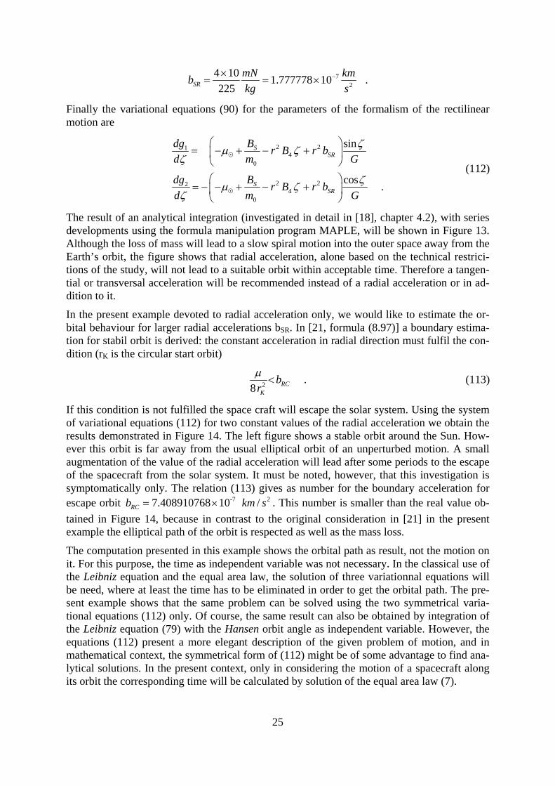
The result of an analytical integration (investigated in detail in [18], chapter 4.2), with series developments using the formula manipulation program MAPLE, will be shown in Figure 13. Although the loss of mass will lead to a slow spiral motion into the outer space away from the Earth’s orbit, the figure shows that radial acceleration, alone based on the technical restrici-tions of the study, will not lead to a suitable orbit within acceptable time. Therefore a tangen-tial or transversal acceleration will be recommended instead of a radial acceleration or in ad-dition to it.

In the present example devoted to radial acceleration only, we would like to estimate the or-bital behaviour for larger radial accelerations bSR. In [21, formula (8.97)] a boundary estima-tion for stabil orbit is derived: the constant acceleration in radial direction must fulfil the con-dition (rK is the circular start orbit)

2

.8 RC

K

br

(113)

If this condition is not fulfilled the space craft will escape the solar system. Using the system of variational equations (112) for two constant values of the radial acceleration we obtain the results demonstrated in Figure 14. The left figure shows a stable orbit around the Sun. How-ever this orbit is far away from the usual elliptical orbit of an unperturbed motion. A small augmentation of the value of the radial acceleration will lead after some periods to the escape of the spacecraft from the solar system. It must be noted, however, that this investigation is symptomatically only. The relation (113) gives as number for the boundary acceleration for escape orbit -7 27.408910768 10 /RCb km s . This number is smaller than the real value ob-

tained in Figure 14, because in contrast to the original consideration in [21] in the present example the elliptical path of the orbit is respected as well as the mass loss.

The computation presented in this example shows the orbital path as result, not the motion on it. For this purpose, the time as independent variable was not necessary. In the classical use of the Leibniz equation and the equal area law, the solution of three variationnal equations will be need, where at least the time has to be eliminated in order to get the orbital path. The pre-sent example shows that the same problem can be solved using the two symmetrical varia-tional equations (112) only. Of course, the same result can also be obtained by integration of the Leibniz equation (79) with the Hansen orbit angle as independent variable. However, the equations (112) present a more elegant description of the given problem of motion, and in mathematical context, the symmetrical form of (112) might be of some advantage to find ana-lytical solutions. In the present context, only in considering the motion of a spacecraft along its orbit the corresponding time will be calculated by solution of the equal area law (7).

26

Figure 13: orbital path of interplanetary space probe with radial acceleration only due to solar attraction, solar pressure, ion thrusters. Inner (green) curve: Earth orbit used as starting curve

Figure 14: orbital path of interplanetary space probe with radial acceleration only due to solar attraction, solar pressure, constant impuls by ion thrusters. Left figure: stable orbit around Sun (in the center of the coordinate system) with constant radial acceleration 7 2

SRb = 7.35 10 /km s , right figure: escape orbit for constant radial

acceleration 7 2SRb = 7.36 10 /km s

5 Adaptation of any Motion to any other Motion

In extension of the previous considerations, a general solution of the variational equations of any motion might be solved in the following way: based on any acceleration under considera-tion, the variational equations are derived corresponding to this acceleration. Their solution

27

leads to a special curve fulfilling the conditions of the given acceleration. Taking into account any other acceleration, new variational equations will be found based on the given curve and triggered by the new acceleration. The solution of these equations will lead to a new curve fulfilling the condition of the previously respected accelerations. In this manner, a step by step procedure (this is not an iteration process!) will lead to a solution of the whole given problem of motion. (This procedure will be explained in detail in a separate paper.) By a suit-able application of such a procedure the target would be to obtain as far as possible an analyt-ical solution by the aid of a modern Computer Algebra System (CAS, see e.g. [21]) before finding the final solution of the given problem by numerical procedures.

6 Conclusions

(1) Rectilinear motion can be adapted to any motion. There are no parameter singularities (besides of special cases in the relation of the motion to a fundamental basic system).

(2) If a curve along which a body is moving is given by its polar equation, and if the area pa-rameter is known, then the acceleration producing this motion can be computed based on the general Leibniz equation (as demonstrated in example 4.1).

(3) A tangent at any curve is the simplest form of a tangential space: a tangential space at any primary space is known to be Euclidean even if the primary space is not Euclidean. Therefore, a generalization of adaptation using rectilinear motion to more general description of motions can be envisaged.

(4) With respect to a Hansen system, with the Hansen orbit angle as given in the equal area law, the rectilinear motion has the radius

.cos P

Gr

V

(5) The general distance law, with relation to a Hansen system with orbit angle and rectile-nar motion with pericentre angle P, has the form

1.

cos P

GV

r

(6) The adaptation of any motion by means of the equations of rectilinear motion with param-eters 1 2cos , sinP Pg V g V , has as a consequence of the Lagrange constraint (66) and

the Leibniz equation in the formulae (53) the in-plane variational equations

21

2

1 2

22

2

1 2

( sin cos )( sin cos )

cos sin

( cos sin )( cos sin ) .

cos sin

R TR T

R TR T

dg r G b bb b

d G g g

dg r G b bb b

d G g g

(7) The out-of-plane variational equation of the space rotation angle , as well as the variation of the equal area parameter G and, finally, the relation to time is given by

3 3

2 2, , .T N

dG r d r Gb b

d G d G r

28

7 References

[1] MANSFELD, J. (1987): Die Vorsokratiker, Griechisch/Deutsch, Auswahl der Fragmente, Übersetzung und Erläuterungen, Philipp Reclam Jun., Stuttgart

[2] DIELS, N. (1957): Die Fragmente der Vorsokratiker, rowohlts Klassiker Nr. 10, Hamburg

[3] ARISTOTELES (1986): in 23 volumes, Vol. VI On the Heavens, with an English translation by W. K. C. Guth-rie, Loeb Classical Library, Cambridge Mass., Harvard University Press, London, William Heinemann Ltd.

[4] DRAKE, S. (1990): 'Newtons Apfel und Galileis "Dialog" ', in: Newtons Universum, Materialien zur Ge-schichte des Kraftbegriffs, Verständliche Forschung, Spektrum der Wissenschaft, Heidelberg, 1990, 116–123

[5] JOCHIM, E. F. M. (2015): ' The Circle will be Closed Now, Finally (On the Inability to Adapt Circular Mo-tions)', Journal of Space Operations and Commutator, April 02, 2015, Vol. 12 Issue 2, ISSN 2410-0005

[6] JOCHIM, E. F. M. (2012/a): 'The Significance of the Hansen-Ideal Space Frame', Astr. Nachr. / AN 333, No. 8, 774-783 (2012) / DOI 10.1002/asna.202222711

[7] LEIBNIZ, G. W. (1689): 'Tentamen de Motuum Coelestium Causis', Acta Eruditorum, Feb 1689, pp. 82-96

[8] AITON, E. J. (1960): 'The Celestial Mechanics of Leibniz', Annals of Science, 16, No. 2, 65–82, (published August 1962)

[9] VOLK, O. (1983): 'Eulers Beiträge zur Theorie der Bewegungen der Himmelskörper', in: Leonhard Euler 1707–1783, Beiträge zu Leben und Werk, Gedenkband des Kantons Basel-Stadt, 1983 Birkhäuser Verlag Basel, 345–362

[10] BIALAS, V. (1998): Vom Himmelsmythos zum Weltgesetz – Eine Kulturgeschichte der Astronomie, Ibera Verlag, Wien, ISBN 3 900436 52 5

[11] VOLK, O. (1976): 'Miscellania from the History of Celestial Mechanics', Celest. Mech. 14, 365–382

[12] SCHAUB, W. (1952): 'Die himmelsmechanischen Grundlagen der Raumfahrt, das Zweikörperproblem und die lösbaren Fälle des Dreikörperproblems', in: Gartmann, H., her.: Raumfahrtforschung, Verlag von R. Oldenbourg, München 1952, pp. 27–115.

[13] RODRIGUES, O. (1840): 'Des lois géométriques qui régissent les déplacements d’un système solide dans l’espace, et la variation des coordonnées provenant de ses déplacements considérés indépendamment des causes qui peuvent les produire', Journal de Mathématiques Pures et Appliquées, 5, 380–440

[14] GRAY, JEREMY J, (1980): 'Olinde Rodrigues’ Paper of 1840 on Transformation Groups', Archive for History of Exact Sciences, 21, Springer Verlag, pp 375-385

[15] DEPRIT, A. (1975): 'Ideal Elements for Perturbed Keplerian Motions', Journal of Research of the National Bureau of Standards - B. Mathematical Sciences. 79B , Nos. 1 and 2, January - June 1975, pp. 1-15

[16] AITON, E. J. (1969): 'Kepler’s Second Law of Planetary Motion', Isis 60, 75–90

[17] FITZPATRICK, PHILIP, M. (1970): Principles of Celestial Mechanics, Academic Press, New York and Lon-don

[18] JOCHIM, E.F.M. (2011): 'Die Verwendung von Hansen-Systemen in Himmelsmechanik und Astrodynamik', German Aerospace Centre, ISRN DLR FB 2011-04

[19] PALACIOS, M, and C. CALVO (1996): 'Ideal Frames and Regularization in Numerical Orbit Computation', The Journal of the Astronautical Sciences, 44, No. 1, January-March, pp. 63-77

[20] ECKSTEIN, M. C., JOCHIM, E. F., LEIBOLD, A. F., LORENZ, J. K., PIETRASS, A. E. (1983): 'Design and Naviga-tion Accuracy Assessment of an Ion Drive Asteroids Flyby and Rendezvous Mission Launched by Ari-ane 4 APEX Demonstration Flight', DFVLR, German Space Operations Center, Oberpfaffenhofen, Inter-nal Report GSOC 83-1, October 11th, 1983

[21] BATTIN, R. H. (1987): An Introduction to the Mathematics and Methods of Astrodynamics, AIAA Educa-tion Series, J. S. Przemieniecki / Series Editor-in-Chief, New York

29

[22] JOCHIM, E. F. M. (2012b): Satellitenbewegung, Band I: Der Bewegungsbegriff [Satellite Motion, Volume I: The Term of Motions], ISSN 1434-8454, ISRN DLR-FB 2012-12, 24. September 2012

[23] JOCHIM, E. F. M. (2012c): Satellitenbewegung, Band II: Bewegung in Raum und Zeit [Satellite Motion, Volume II: Motion in Space and Time], ISSN 1434-8454, ISRN DLR-FB 2012-13, 6. November 2012

[24] JOCHIM, E. F. M. (2013): Satellitenbewegung, Band V: Die Verknüpfung von Bewegung und Beobach-tungsgeometrie [Satellite Motion, Volume V: The Combination of Motion and Observational Geometry], ISSN 1434-8454, ISRN DLR-FB 2013-12, 26. Juni 2013

[25] JOCHIM, E. F. M. (2014): Satellitenbewegung, Band III: Natürliche und gesteuerte Bewegung [Satellite Motion, Volume III: Natural and Controlled Motion], ISSN 1434-8454, ISRN DLR-FB 2014-36, 28. November 2014

Acknowledgments:

The author cordially thanks Prof. Dr. Bernd Häusler (Uni BW München) for valuable advice with respect to the example in radial acceleration and to Mr. Colin Ward for support in the compilation of this paper.

Printed on 2016-01-28, 10:14