recursive partitioning for modelling survey · pdf filean introduction to the r package: rpms....
TRANSCRIPT

Daniell Toth
U.S. Bureau of Labor Statistics
Content represents the opinion of the authors only.
Recursive Partitioning for
Modelling Survey data
An Introduction to the R package: rpms

Talk Outline
Brief introduction of recursive partitioning
Description of simulated data used for demonstrations
Demonstrate some of the functionality of the rpms package:
tree regression with rpms
including sample design information
examples using provided functions
Example Using Consumer Expenditure Data

Recursive Partitioning
full dataset
θ
Population has some unknown parameters θ
that we wish to estimate

Recursive Partitioning
full dataset
θ
θ is often the mean, but could be other model parameters
such as variance, proportion or coefficients of a linear model

Recursive Partitioning
full dataset
z1 ≤ a z
1> a
θ θ
θ could be very different for different sub-domains of the population
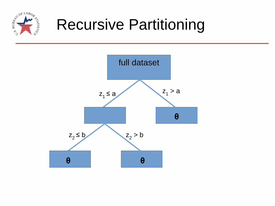
Recursive Partitioning
full dataset
z1 ≤ a z
1> a
z2 ≤ b z
2> b
θθ
θ

Recursive Partitioning
full dataset
z1 ≤ a z
1> a
z2 ≤ b z
2> b
θ
θ
θ
z3 ≤ c z
3> c
θ
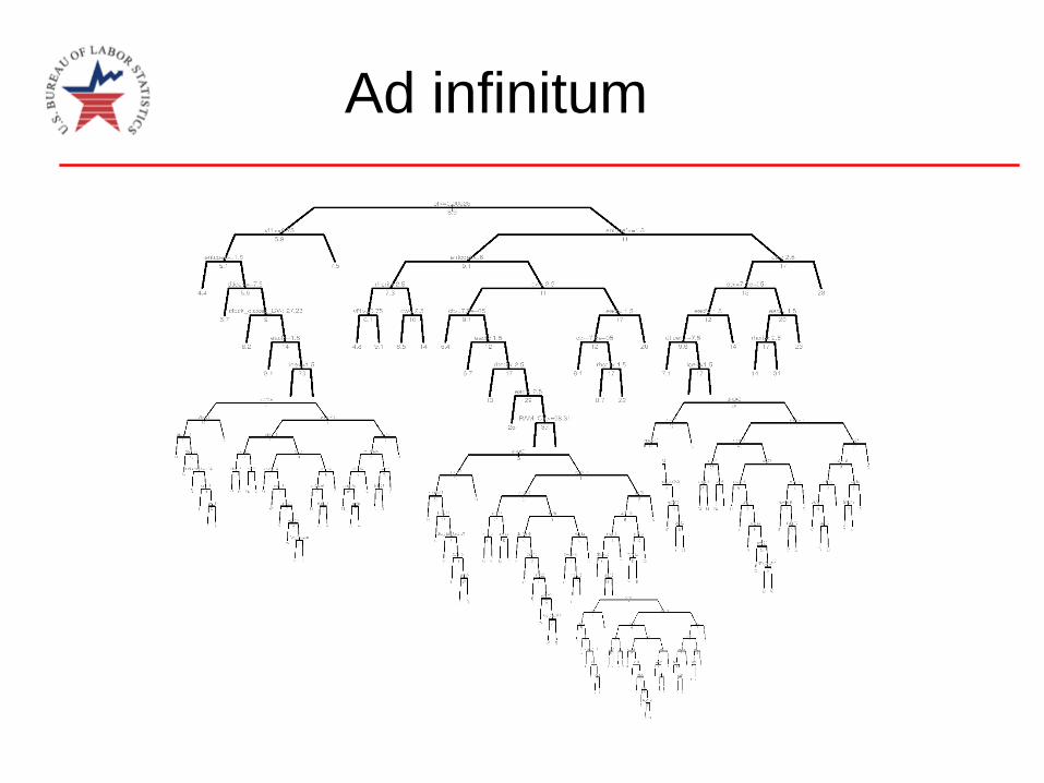
Ad infinitum

The Problem
We wish to understand the relationship between a variable Y and
number of other available variables in X and Z
(Y, X, Z) come from a complex sample
Y ~ X linear relationship (parametric)
XTβ ~ Z unknown and complicated (nonparametric)
Z contains many variables (large p);
Xtβ depends on subset of Z and interactions (variable selection)
Some variables in Z maybe collinear
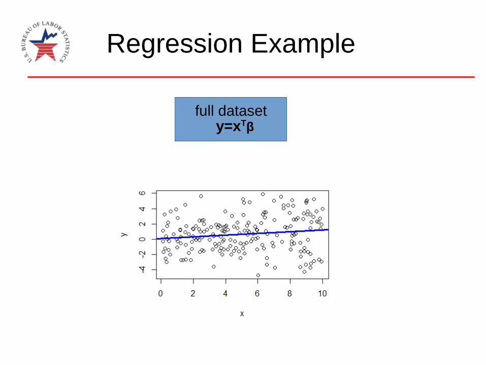
Regression Example
full datasety=xTβ
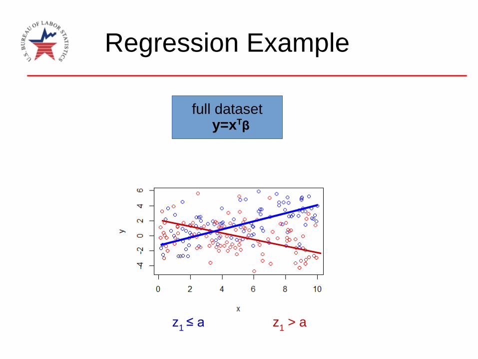
Regression Example
full datasety=xTβ
z1 ≤ a z
1> a

Regression Example
full dataset
z1 ≤ a z
1> a
y=xTβ2y=xTβ
1

CRAN – Package rpms

The rpms package
>library(rpms)
Package provides a number of functions designed to help
model and analyze survey data using design-consistent
regression trees.
rpms - returns rpms object
methods:
print, predict
other available functions:
node_plot, qtree, in_node

The Simulated Data
We simulate a dataset of 10,000 observations simd
yij
= f(xij,
vij) + η
j+ ε
ij
x = continuous variable
va,
vb,
… vf
= categorical variables
va
is the only variable that f depends on

The Simulated Data
We simulate a dataset of 10,000 observations simd
yij
= f(xij, v
ij) + η
j+ ε
ij
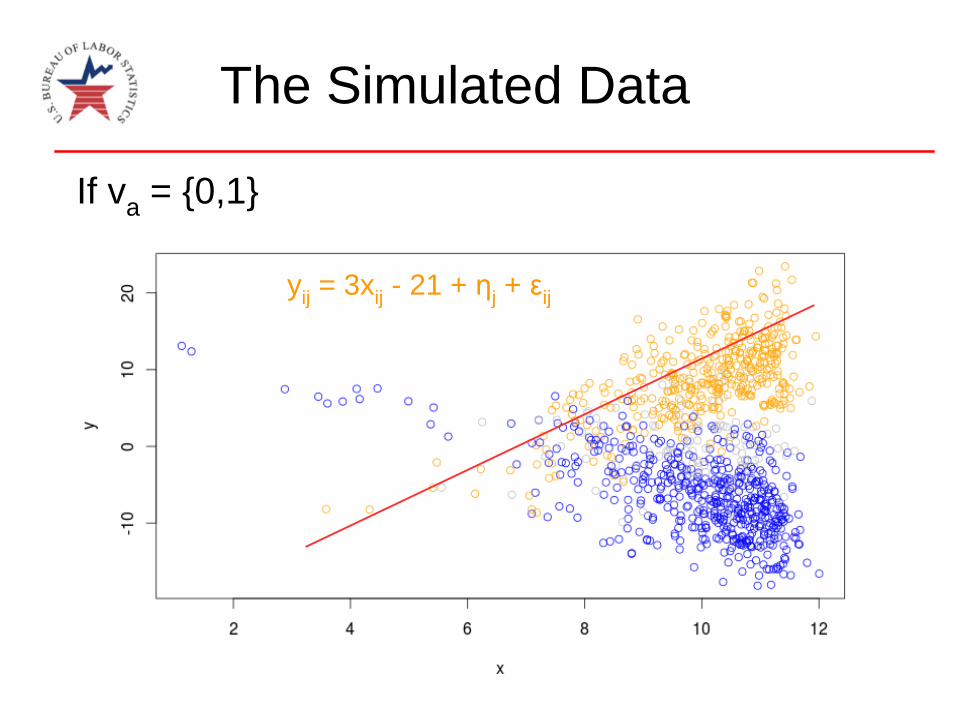
The Simulated Data
yij
= 3xij
- 21 + ηj+ ε
ij
If va
= {0,1}

The Simulated Data
yij
= -2xij
+ 14 + ηj+ ε
ij
If

The Simulated Data
We simulate a dataset of 10,000 observations simd
yij
= f(xij, v
ij) + η
j+ ε
ij
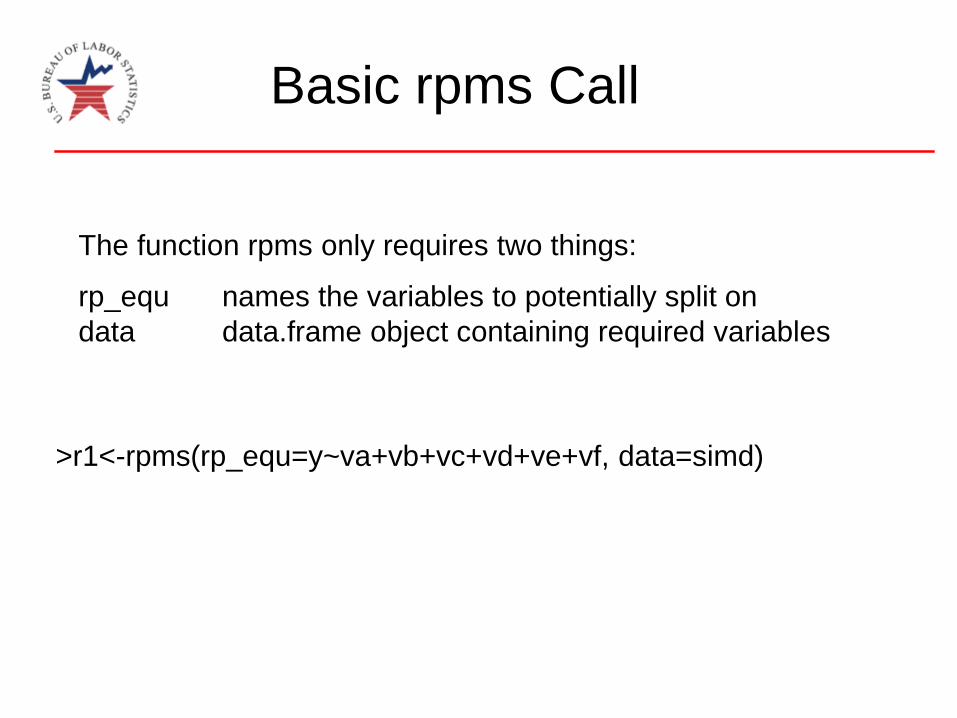
Basic rpms Call
The function rpms only requires two things:
rp_equ names the variables to potentially split on
data data.frame object containing required variables
>r1<-rpms(rp_equ=y~va+vb+vc+vd+ve+vf, data=simd)

Basic rpms Call
The function rpms only requires two things:
rp_equ names the variables to potentially split on
data data.frame object containing required variables
R formula
>iid <-rpms(rp_equ=y~va+vb+vc+vd+ve+vf, data=simd[s,])

Basic rpms Call
The function rpms only requires two things:
rp_equ names the variables to potentially split on
data data.frame object containing required variables
R formula
data set containing:
1.) splitting variables,
2.) model variables,
may contain:
3.) design variables
>iid <-rpms(rp_equ=y~va+vb+vc+vd+ve+vf, data=simd[s,])

Basic rpms Call
The function rpms only requires two things:
rp_equ names the variables to potentially split on
data data.frame object containing required variables
splitting variables
seperated by +
>iid <-rpms(rp_equ=y~va+vb+vc+vd+ve+vf, data=simd[s,])

Basic rpms Call
The function rpms only requires two things:
rp_equ names the variables to potentially split on
data data.frame object containing required variables
iid is an rpms object
R assignment operator
>iid <-rpms(rp_equ=y~va+vb+vc+vd+ve+vf, data=simd[s,])

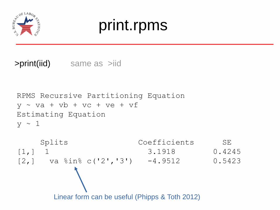
print.rpms
>print(iid) same as >iid
RPMS Recursive Partitioning Equation
y ~ va + vb + vc + ve + vf
Estimating Equation
y ~ 1
Splits Coefficients SE
[1,] 1 3.1918 0.4245
[2,] va %in% c('2','3') -4.9512 0.5423

print.rpms
>print(iid) same as >iid
RPMS Recursive Partitioning Equation
y ~ va + vb + vc + ve + vf
Estimating Equation
y ~ 1
Splits Coefficients SE
[1,] 1 3.1918 0.4245
[2,] va %in% c('2','3') -4.9512 0.5423
no e_eq
fits mean by
default
print.rpms
>print(iid) same as >iid
RPMS Recursive Partitioning Equation
y ~ va + vb + vc + ve + vf
Estimating Equation
y ~ 1
Splits Coefficients SE
[1,] 1 3.1918 0.4245
[2,] va %in% c('2','3') -4.9512 0.5423
Linear form can be useful (Phipps & Toth 2012)

Population Parameters
RPMS Recursive Partitioning Equation
y ~ va + vb + vc + ve + vf
Estimating Equation
y ~ 1
Splits Coefficients SE
[1,] 1 3.1918 0.4245
[2,] va %in% c('2','3') -4.9512 0.5423
rpms model on srs n=400
RPMS Recursive Partitioning Equation
y ~ va + vb + vc + vd + ve + vf
Estimating Equation
y ~ 1
Splits Coefficients SE
[1,] 1 2.9317 0.2765
[2,] va %in% c('2','3') -4.5939 0.3354
rpms model on population

Population Parameters
RPMS Recursive Partitioning Equation
y ~ va + vb + vc + ve + vf
Estimating Equation
y ~ 1
Splits Coefficients SE
[1,] 1 3.1918 0.4245
[2,] va %in% c('2','3') -4.9512 0.5423
rpms model on srs n=400
RPMS Recursive Partitioning Equation
y ~ va + vb + vc + vd + ve + vf
Estimating Equation
y ~ 1
Splits Coefficients SE
[1,] 1 2.9317 0.2765
[2,] va %in% c('2','3') -4.5939 0.3354
same split
rpms model on population

Population Parameters
RPMS Recursive Partitioning Equation
y ~ va + vb + vc + ve + vf
Estimating Equation
y ~ 1
Splits Coefficients SE
[1,] 1 3.1918 0.4245
[2,] va %in% c('2','3') -4.9512 0.5423
rpms model on srs n=400
RPMS Recursive Partitioning Equation
y ~ va + vb + vc + vd + ve + vf
Estimating Equation
y ~ 1
Splits Coefficients SE
[1,] 1 2.9317 0.2765
[2,] va %in% c('2','3') -4.5939 0.3354
similar coefficients
rpms model on population

Population Parameters
RPMS Recursive Partitioning Equation
y ~ va + vb + vc + ve + vf
Estimating Equation
y ~ 1
Splits Coefficients SE
[1,] 1 3.1918 0.4245
[2,] va %in% c('2','3') -4.9512 0.5423
rpms model on srs n=400
RPMS Recursive Partitioning Equation
y ~ va + vb + vc + vd + ve + vf
Estimating Equation
y ~ 1
Splits Coefficients SE
[1,] 1 2.9317 0.2765
[2,] va %in% c('2','3') -4.5939 0.3354
higher standard errors
rpms model on population

qtree
Once we have an rpms object we can include its tree structure
as a figure in a Latex paper or Sweave document
>qtree(iid)

qtree
Once we have an rpms object we can include its tree structure
as a figure in a Latex paper or Sweave document
>qtree(iid)
\begin{figure}[ht]
\centering
\begin{tikzpicture}[scale=1, ]
\tikzset{every tree node/.style={align=center,anchor=north}}
\Tree [.{rpms} [.{$va \in \{2,3\}$} {\fbox{node 2} \\ \fbox{value -1.76}}
][.{$va \in \{1,0\}$}
{\fbox{node 3} \\ \fbox{value 3.19}} ]]
\end{tikzpicture}
\caption{}
\end{figure}

qtree

Other options in qtree
qtree takes several optional parameters:
title = character string for naming root node; default="rpms“
label = string for LaTex figure label; used referencing figure,
caption = string caption for figure, defaults to blank
scale= number (0, ∞); changes relative size of figure;
default=1
> qtree(iid, title="iid tree", label="iid_tree",
caption="This is the tree fit from the simple random sample.")
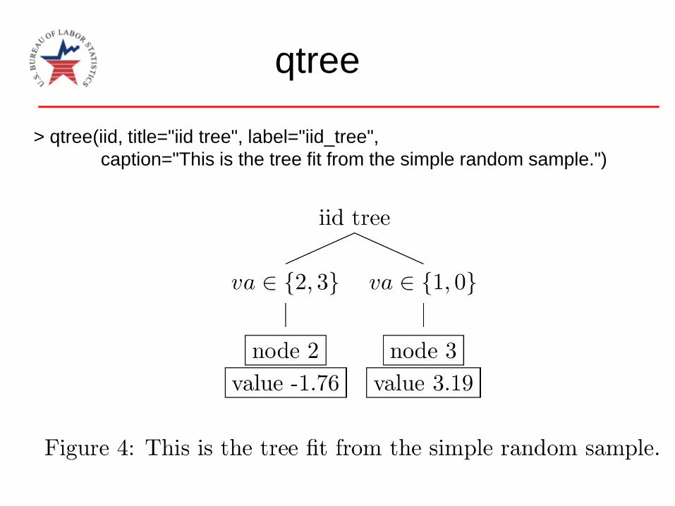
qtree
> qtree(iid, title="iid tree", label="iid_tree",
caption="This is the tree fit from the simple random sample.")

Tree Regression
Instead of estimating the mean of each node, we estimate the
parameters to the equation y = βx + α
>rx1<-rpms(rp_equ=y~va+vb+vc+vd+ve+vf, data=simd
e_equ=y~x)

Tree Regression
Instead of estimating the mean of each node, we estimate the
parameters to the equation y = βx + α
>rx1<-rpms(rp_equ=y~va+vb+vc+vd+ve+vf, data=simd
e_equ=y~x)
estimating
equation

Tree Regression
Instead of estimating the mean of each node, we estimate the
parameters to the equation y = βx + α
>rx1<-rpms(rp_equ=y~va+vb+vc+vd+ve+vf, data=simd
e_equ=y~x)
dependent variable must be the same
for rp_equ and e_equestimating
equation

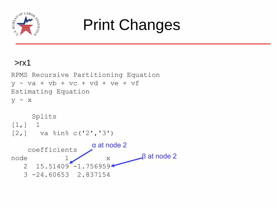
Print Changes
>rx1
e_eq
RPMS Recursive Partitioning Equation
y ~ va + vb + vc + vd + ve + vf
Estimating Equation
y ~ x
Splits
[1,] 1
[2,] va %in% c('2','3')
coefficients
node 1 x
2 15.51409 -1.756959
3 -24.60653 2.837154

Print Changes
>rx1
α at node 2
RPMS Recursive Partitioning Equation
y ~ va + vb + vc + vd + ve + vf
Estimating Equation
y ~ x
Splits
[1,] 1
[2,] va %in% c('2','3')
coefficients
node 1 x
2 15.51409 -1.756959
3 -24.60653 2.837154
Print Changes
>rx1
α at node 2
β at node 2
RPMS Recursive Partitioning Equation
y ~ va + vb + vc + vd + ve + vf
Estimating Equation
y ~ x
Splits
[1,] 1
[2,] va %in% c('2','3')
coefficients
node 1 x
2 15.51409 -1.756959
3 -24.60653 2.837154

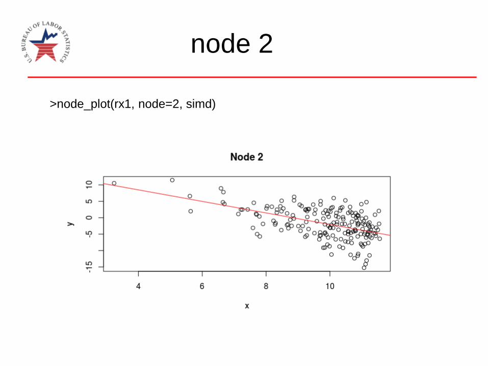
node_plot
This lets you see each node with data and the fitted line
with respect to chosen variable
>node_plot(rx1, node=2, simd)
RPMS Recursive Partitioning Equation
y ~ va + vb + vc + vd + ve + vf
Estimating Equation
y ~ x
Splits
[1,] 1
[2,] va %in% c('2','3')
coefficients
node 1 x
2 15.51409 -1.756959
3 -24.60653 2.837154
rpms
object data

node_plot
This lets you see each node with data and the fitted line
with respect to chosen variable
>node_plot(rx1, node=2, simd,
variable = x)
RPMS Recursive Partitioning Equation
y ~ va + vb + vc + vd + ve + vf
Estimating Equation
y ~ x
Splits
[1,] 1
[2,] va %in% c('2','3')
coefficients
node 1 x
2 15.51409 -1.756959
3 -24.60653 2.837154
Parameter variable defaults
to the first variable of e_eq
node 2
>node_plot(rx1, node=2, simd)

node 3
>node_plot(rx1, node=3, simd)

rx1

Data from a
Complex Sample
The 10,000 observations simd were constructed by simulating
500 clusters with 20 observations each.
yij
= f(xij) + η
j+ ε
ij
x = continuous variable
va,
vb,
… vf
= categorical variables
Data from a
Complex Sample
The 10,000 observations simd we constructed by simulating
500 clusters with 20 observations each.
yij
= f(xij) + η
j+ ε
ij
x = continuous variable
va,
vb,
… vf
= categorical variables
N(0, σc) same for each observation in cluster
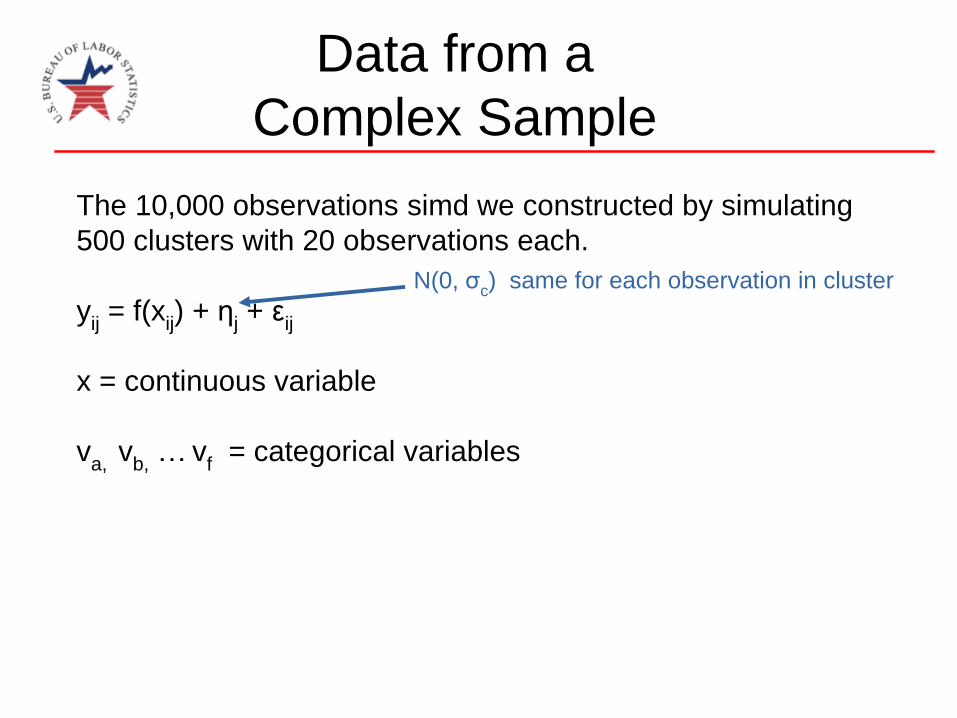
Data from a
Complex Sample
The 10,000 observations simd we constructed by simulating
500 clusters with 20 observations each.
yij
= f(xij) + η
j+ ε
ij
x = continuous variable
va,
vb,
… vf
= categorical variables
N(0, σc) same for each observation in cluster
xj+ e
ij
more homogeneous within cluster

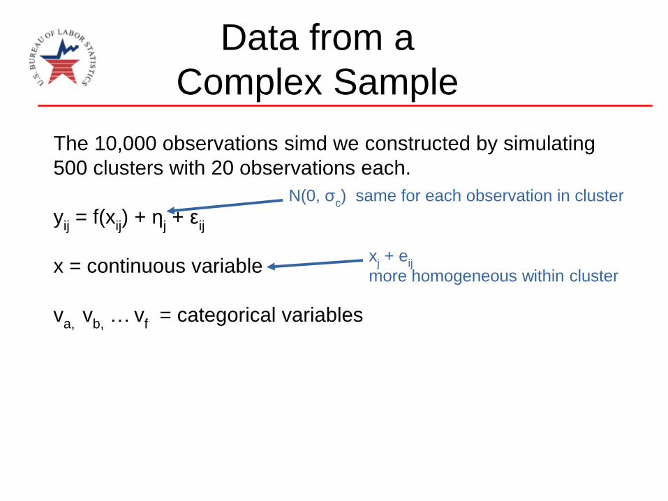
Data from a
Complex Sample
The 10,000 observations simd we constructed by simulating
500 clusters with 20 observations each.
yij
= f(xij) + η
j+ ε
ij
x = continuous variable
va,
vb,
… vf
= categorical variables
N(0, σc) same for each observation in cluster
xj+ e
ij
more homogeneous within cluster
vc
same for every
observation in cluster

Cluster Sample
SRS of clusters
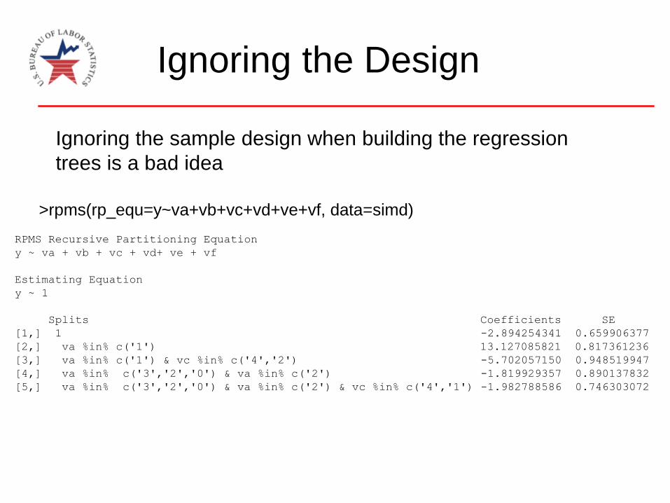
Ignoring the Design
Ignoring the sample design when building the regression
trees is a bad idea
>rpms(rp_equ=y~va+vb+vc+vd+ve+vf, data=simd)
RPMS Recursive Partitioning Equation
y ~ va + vb + vc + vd+ ve + vf
Estimating Equation
y ~ 1
Splits Coefficients SE
[1,] 1 -2.894254341 0.659906377
[2,] va %in% c('1') 13.127085821 0.817361236
[3,] va %in% c('1') & vc %in% c('4','2') -5.702057150 0.948519947
[4,] va %in% c('3','2','0') & va %in% c('2') -1.819929357 0.890137832
[5,] va %in% c('3','2','0') & va %in% c('2') & vc %in% c('4','1') -1.982788586 0.746303072
variable vc included
in model
>rpms(rp_equ=y~va+vb+vc+vd+ve+vf, data=simd,
clusters=~ids)
including psu labels ids

Regression Tree
with Cluster Designaccounting for clusters could change more than standard errors
RPMS Recursive Partitioning Equation
y ~ va + vb + vc + vd + ve + vf
Estimating Equation
Y ~ 1
Splits Coefficients SE
[1,] 1 2.56736 1.63061
[2,] va %in% c('2','3') -1.86798 2.22432

Cluster Design vs iidRPMS Recursive Partitioning Equation
y ~ va + vb + vc + vd + ve + vf
Estimating Equation
Y ~ 1
Splits Coefficients SE
[1,] 1 2.56736 1.63061
[2,] va %in% c('2','3') -1.86798 2.22432
> iid
RPMS Recursive Partitioning Equation
y ~ va + vb + vc + ve + vf
Estimating Equation
y ~ 1
Splits Coefficients SE
[1,] 1 3.1918 0.4245
[2,] va %in% c('2','3') -4.9512 0.5423
correct tree model

Cluster Design vs iidRPMS Recursive Partitioning Equation
y ~ va + vb + vc + vd + ve + vf
Estimating Equation
Y ~ 1
Splits Coefficients SE
[1,] 1 2.56736 1.63061
[2,] va %in% c('2','3') -1.86798 2.22432
> iid
RPMS Recursive Partitioning Equation
y ~ va + vb + vc + ve + vf
Estimating Equation
y ~ 1
Splits Coefficients SE
[1,] 1 3.1918 0.4245
[2,] va %in% c('2','3') -4.9512 0.5423
coefficients aren’t
as accurate

Cluster Design vs iidRPMS Recursive Partitioning Equation
y ~ va + vb + vc + vd + ve + vf
Estimating Equation
Y ~ 1
Splits Coefficients SE
[1,] 1 2.56736 1.63061
[2,] va %in% c('2','3') -1.86798 2.22432
> iid
RPMS Recursive Partitioning Equation
y ~ va + vb + vc + ve + vf
Estimating Equation
y ~ 1
Splits Coefficients SE
[1,] 1 3.1918 0.4245
[2,] va %in% c('2','3') -4.9512 0.5423
standard errors of
coefficients DID increase

Unequal Probability
of Selection

Unequal Probability
of Selection
Draw sample with
probability of
selection
proportional to

Unequal Probability
of Selection
x
selected points

Trees Under Unequal
Probability of Selection
rpms(y~va+vb+vc+ve+vf, data=simd,
e_eq=y~x)
>rpms(y~va+vb+vc+vd+ve+vf, data=simd,
e_eq=y~x, weights=1/pi_i)
Ignore Weight
RPMS Recursive Partitioning Equation
y ~ va + vb + vc + ve + vf
Estimating Equation
y ~ x
Splits
[1,] 1
[2,] va %in% c('2','3')
coefficients
node 1 x
2 26.94646 -2.99273
3 -21.78096 2.46555
RPMS Recursive Partitioning Equation
y ~ va + vb + vc + ve + vf
Estimating Equation
y ~ x
Splits
1
va %in% c('2','3')
va %in% c('2','3') & vc %in% c('4','3','1','0')
coefficients
node 1 x
4 16.100792 -2.218358
5 9.708693 -1.587803
3 -17.017023 2.384377
includes vc

Trees Under Unequal
Probability of Selection
rpms(y~va+vb+vc+ve+vf, data=simd,
e_eq=y~x)
>rpms(y~va+vb+vc+vd+ve+vf, data=simd,
e_eq=y~x, weights=1/pi_i)
Ignore Weight
RPMS Recursive Partitioning Equation
y ~ va + vb + vc + ve + vf
Estimating Equation
y ~ x
Splits
[1,] 1
[2,] va %in% c('2','3')
coefficients
node 1 x
2 26.94646 -2.99273
3 -21.78096 2.46555
RPMS Recursive Partitioning Equation
y ~ va + vb + vc + ve + vf
Estimating Equation
y ~ x
Splits
1
va %in% c('2','3')
va %in% c('2','3') & vc %in% c('4','3','1','0')
coefficients
node 1 x
4 16.100792 -2.218358
5 9.708693 -1.587803
3 -17.017023 2.384377
correct model

Predict Method
Predict Method
> predict(rx1, newdata)

Predict Method
> predict(rx1, newdata)
object of type rpms

Predict Method
> predict(rx1, newdata)
dataframe containing all variables
on the right hand side of rp_equ
and e_equ

Predict Method
> predict(rx1, newdata)
> pre1 <- sample(10000, 8)
> new <- as.data.frame.array(simd[pre1, -c(1, 2, 10)],
row.names=1:8)
> new[,"x"] <- round(new[,"x"], 2)
>
> predict(iid, newdata=new)
[1] 3.191847 3.191847 3.191847 3.191847 3.191847 -1.759392
3.191847 3.191847

Domain Estimates
rpms models can be used for domain estimates using predict
Domain: x < 9

Domain Estimates
rpms models can be used for domain estimates using predict
Domain: x < 9
D <- which(simd[,"x"]<9)
mean(predict(rxp, simd[D,])) + est_res

Domain Estimates
rpms models can be used for domain estimates using predict
Domain: x < 9
D <- which(simd[,"x"]<9)
mean(predict(rxp, simd[D,])) + est_res
predicted population values

Domain Estimates
rpms models can be used for domain estimates using predict
Domain: x < 9
D <- which(simd[,"x"]<9)
mean(predict(rxp, simd[D,])) + est_res
HT estimate of
population residuals

Domain Estimates
Domain: x < 9
Mean of HT estimate: -0.7300458
Mean using predict : -0.7710101
rpms models can be used for domain estimates using predict
over 500 samples

Domain Estimates
Domain: x < 9
Mean of HT estimate: -0.7300458
Mean using predict : -0.7710101
Population mean: -0.7622469
rpms models can be used for domain estimates using predict
over 500 samples

Domain Estimates
estimator using predict
sd = 0.5434727
usual HT estimator
sd = 1.019409

Other rpms Options

Other rpms Options
rpms has a number of other optional arguments:
l_fn loss-function written in R
bin_size minimum number of observations in each node
pval p-value used to reject null hypothesis

CE Data

CE Data
data(CE)
FSALARYX: Income from Salary
FINCBTAX: Income Before Tax
FINDRETX: Amount put in an individual retirement plan
FAM_SIZE: Number of members
NO_EARNR: Number of earners
PERSOT64: Number of people >64 yrs old
CUTENURE: 1 Owned with mortgage; 2-6 Other
VEHQ: Number of owned vehicles
REGION: 1 Northeast; 2 Midwest; 3 South; 4 West

CE Example
workers = CE[which(CE$FSALARYX>0 & CE$FINCBTAX<600000), ]

CE Example
workers = CE[which(CE$FSALARYX>0 & CE$FINCBTAX<600000), ]
Households with income from salary
and
Income < $600,000

CE Example
workers = CE[which(CE$FSALARYX>0 & CE$FINCBTAX<600000), ]
subset of
CE datasetHouseholds with income from salary
and
Income < $600,000

CE Example
workers = CE[which(CE$FSALARYX>0 & CE$FINCBTAX<600000), ]
workers$saver = ifelse(workers$FINDRETX>0, 1, 0)
new variable
1 if has retirement savings
0 otherwise

CE Example
workers = CE[which(CE$FSALARYX>0 & CE$FINCBTAX<600000), ]
workers$saver = ifelse(workers$FINDRETX>0, 1, 0)
rpms(rp_equ=saver~FAM_SIZE+NO_EARNR+CUTENURE+VEHQ+REGION,
e_equ = saver~FINCBTAX,
weights=~FINLWT21, clusters=~CID, data=workers, pval=.01)

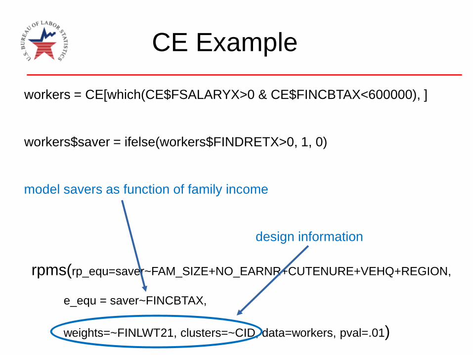
CE Example
workers = CE[which(CE$FSALARYX>0 & CE$FINCBTAX<600000), ]
workers$saver = ifelse(workers$FINDRETX>0, 1, 0)
model savers as function of family income
rpms(rp_equ=saver~FAM_SIZE+NO_EARNR+CUTENURE+VEHQ+REGION,
e_equ = saver~FINCBTAX,
weights=~FINLWT21, clusters=~CID, data=workers, pval=.01)
CE Example
workers = CE[which(CE$FSALARYX>0 & CE$FINCBTAX<600000), ]
workers$saver = ifelse(workers$FINDRETX>0, 1, 0)
model savers as function of family income
design information
rpms(rp_equ=saver~FAM_SIZE+NO_EARNR+CUTENURE+VEHQ+REGION,
e_equ = saver~FINCBTAX,
weights=~FINLWT21, clusters=~CID, data=workers, pval=.01)

CE Example
CE Example
RPMS Recursive Partitioning Equation
saver ~ FAM_SIZE + NO_EARNR + PERSOT64 + CUTENURE + VEHQ + REGION
Estimating Equation
saver ~ FINCBTAX
Splits
[1,] 1
[2,] CUTENURE %in% c('1')
[3,] CUTENURE %in% c('4','2','5','6') & FAM_SIZE <= 2
coefficients
node 1 FINCBTAX
2 0.068209137 7.805248e-07
6 0.011400909 1.548897e-06
7 -0.004685768 8.678787e-07
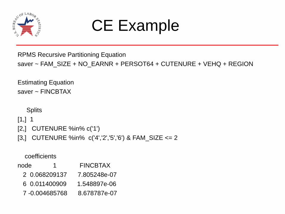

CE Example

CE Example
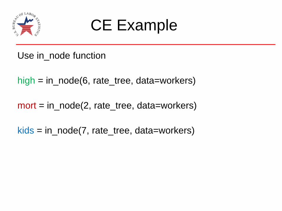
Use in_node function
high = in_node(6, rate_tree, data=workers)

CE Example
Use in_node function
high = in_node(6, rate_tree, data=workers)
index of observations
in a given node
node
rpms
object
could be
new data

CE Example
Use in_node function
high = in_node(6, rate_tree, data=workers)
index of observations
in a given node
node
rpms
object
could be
new data
Can be used to analyze groups separately
Example: summary(workers[high, ])
CE Example
Use in_node function
high = in_node(6, rate_tree, data=workers)
mort = in_node(2, rate_tree, data=workers)
kids = in_node(7, rate_tree, data=workers)

CE Example

Wrap Up
We have introduced the rpms package and demonstrated a
number of functions including

Wrap Up
We have introduced the rpms package and demonstrated a
number of functions including
The package does NOT yet: have a general plot function
handle missing values

Wrap Up
We have introduced the rpms package and demonstrated a
number of functions including
The package does NOT yet: have a general plot function
handle missing values
This is a working package: version: 0_2_0

Wrap Up
We have introduced the rpms package and demonstrated a
number of functions including
The package does NOT yet: have a general plot function
handle missing values
This is a working package: version: 0_2_0 Lots of features are experimental and being tested (don’t use)
May have bugs (weights not used in variable selection in 0_2_0)
Working on more features and applications
Open to taking suggestions
Note the 0

Wrap Up
We have introduced the rpms package and demonstrated a
number of functions including
The package does NOT yet: have a general plot function
handle missing values
This is a working package: version: 0_2_0 Lots of features are experimental and being tested (don’t use)
May have bugs (weights not used in variable selection in 0_2_0)
Working on more features and applications
Open to taking suggestions
Look for version 0_3_0 in early April
Note the 0
