recycling krylov subspaces for …mlparks/papers/krylovrecycling.pdfkrylov subspace recycling 1653...

SIAM J. SCI. COMPUT. c© 2006 Society for Industrial and Applied MathematicsVol. 28, No. 5, pp. 1651–1674

RECYCLING KRYLOV SUBSPACES FOR SEQUENCES OFLINEAR SYSTEMS∗

MICHAEL L. PARKS† , ERIC DE STURLER‡ , GREG MACKEY§ , DUANE D. JOHNSON¶,

AND SPANDAN MAITI‖

Abstract. Many problems in science and engineering require the solution of a long sequenceof slowly changing linear systems. We propose and analyze two methods that significantly reducethe total number of matrix-vector products required to solve all systems. We consider the generalcase where both the matrix and right-hand side change, and we make no assumptions regardingthe change in the right-hand sides. Furthermore, we consider general nonsingular matrices, andwe do not assume that all matrices are pairwise close or that the sequence of matrices convergesto a particular matrix. Our methods work well under these general assumptions, and hence forma significant advancement with respect to related work in this area. We can reduce the cost ofsolving subsequent systems in the sequence by recycling selected subspaces generated for previoussystems. We consider two approaches that allow for the continuous improvement of the recycledsubspace at low cost. We consider both Hermitian and non-Hermitian problems, and we analyzeour algorithms both theoretically and numerically to illustrate the effects of subspace recycling. Wealso demonstrate the effectiveness of our algorithms for a range of applications from computationalmechanics, materials science, and computational physics.

Key words. sequence of linear systems, linear solvers, Krylov methods, truncation, restarting,Krylov subspace recycling, iterative methods

AMS subject classifications. 65F10, 65N22

DOI. 10.1137/040607277

1. Introduction. We consider the solution of a long sequence of general linearsystems

A(i)x(i) = b(i), i = 1, 2, . . . ,(1.1)

where the matrix A(i) ∈ Cn×n and right-hand side b(i) ∈ C

n change from one systemto the next, and the systems are typically not available simultaneously. Such sequencesarise in many problems.

∗Received by the editors April 24, 2004; accepted for publication (in revised form) February 16,2006; published electronically October 6, 2006.

http://www.siam.org/journals/sisc/28-5/60727.html†Department of Computer Science, University of Illinois at Urbana-Champaign, Urbana, IL 61801,

and Computational Mathematics and Algorithms, Sandia National Laboratories, P.O. Box 5800, MS1110, Albuquerque, NM 87185 ([email protected]). Sandia is a multiprogram laboratory operatedby Sandia Corporation, a Lockheed Martin Company, for the United States Department of Energyunder contract DE-AC04-94-AL85000. The work of this author was supported by the ComputationalScience and Engineering program at UIUC through two CSE fellowships.

‡Department of Mathematics, Virginia Tech, Blacksburg, VA 24061-0123 ([email protected]). Thework of this author was supported by the Materials Computation Center (UIUC) through grantsNSF DMR 99-76550 and DMR-0325939, and by the Center for Simulation of Advanced Rockets(UIUC) through grant DOE LLNL B341494.

§Department of Computer Science, University of Illinois at Urbana-Champaign, Urbana, IL 61801(currently [email protected]). The work of this author was supported by the Center for Simulationof Advanced Rockets through grant DOE LLNL B341494.

¶Department of Materials Science, University of Illinois at Urbana-Champaign, Urbana, IL 61801([email protected]). The work of this author was supported through the Materials ComputationCenter through grant NSF DMR 99-76550.

‖Department of Aerospace Engineering, University of Illinois at Urbana-Champaign, Urbana, IL61801 ([email protected]).

1651

1652 PARKS, DE STURLER, MACKEY, JOHNSON, MAITI

One important class of applications that we consider occurs in modeling fatigueand fracture via finite element analysis. These analyses use dynamic loading, requir-ing many loading steps, and rely on implicit solvers [13]. Generally, several thousandloading increments, each corresponding to a linear system, are required to resolvethe fracture progression. The matrix and right-hand side, at each loading step, de-pend on the previous solution, so that only one linear system is available at a time.Further, the solution vectors are updates to a displacement vector and are thereforeuncorrelated. Although the change from one linear system to the next is small, thecumulative change after many loading increments is significant. Rather than discard-ing the Krylov space generated when solving a linear system, we judiciously select asubspace and use it to reduce the number of iterations for solving the next system. Werefer to this process as Krylov subspace recycling. Clearly, similar sequences of linearsystems arise from other (nonlinear) time-dependent applications. Another importantsource of such sequences of linear systems are Newton or Broyden-type methods forsolving nonlinear equations and optimization problems.

We consider methods for the solution of sequences of general matrices, and do notassume that all matrices are pairwise close or that the sequence of matrices convergesto a particular matrix. In addition, we make no assumptions on the right-hand-sidevectors. A method that is effective under these assumptions must satisfy a numberof properties. First, the method must be able to identify and converge to an effectivesubspace for recycling (the recycle space) in a reasonable number of iterations, andit must be able to converge to an effective recycle space over the solution of multiplelinear systems. Otherwise, a good recycle space may never be found for a sequence ofchanging matrices. Second, for efficiency a significant convergence improvement forthe linear solver must be obtained with a relatively small recycle space. Third, themethod must be able to converge quickly to an effective perturbed recycle space for anupdated matrix, and it must provide an inexpensive mechanism for regularly updatingthe recycle space to reflect the changes in the linear systems. As we will show, ourproposed methods satisfy these properties, and they are effective under these generalassumptions. As such, they form a significant advancement with respect to relatedwork in this area.

We consider two approaches for the solution of (1.1) which are related to two ex-isting truncated and restarted solvers. These solvers, GMRES-DR [21] and GCROT[7], were developed for solving single linear systems; both recycle a judiciously se-lected subspace between restarts to maintain good convergence. In the following, wedefine a truncation in the sense used by GCROT, wherein the iteration is restartedwith a selected subspace and each new vector generated is orthogonalized againstthis subspace. We define a cycle as the computation between truncations or restarts.The first approach is to recycle an approximate invariant subspace and use it fordeflation, following the GMRES-DR method. Since GMRES-DR cannot be adaptedfor recycling, we propose a more general method, GCRO-DR. The work by Rey andRisler [25, 26] has a similar motivation as that for GMRES-DR; see below. However,our implementation is cheaper, more effective, and more adaptive. An alternativeidea is to recycle a subspace that minimizes the loss of orthogonality with the Krylovsubspace from the previous system [7]. In either case, the recycled subspace will beutilized by first minimizing the residual over this subspace and then maintaining or-thogonality with the image of this space in the Arnoldi recurrence. We will show thatsubspaces that are useful to retain for a subsequent cycle when solving a single linearsystem are also useful for the next linear system in a sequence if the matrix does

KRYLOV SUBSPACE RECYCLING 1653

not change significantly. The proposed methods can be tuned to recycle a variety ofsubspaces based on computed information from the matrix, background knowledge ofthe application, and other information; this is discussed in [15]. However, for a firstevaluation, it is reasonable to analyze the effectiveness of these existing methods ap-propriately modified for solving (1.1). The application of these methods to sequencesof linear systems where both matrix and right-hand side change is new and providesa significant advance on related methods discussed below. Our proposed methodsoffer an efficient mechanism for continuous updating of the recycled subspace. As aresult, they quickly adapt to gradual changes in matrices. Further, they make fewassumptions on the linear systems and are applicable to general matrices. In addition,we provide theoretical motivation and careful experimental analysis of these methods.Our results show that significant convergence improvements are obtained using recy-cled subspaces of a small dimension. The application of an early version of GCROTto multiple right-hand sides was briefly discussed in [5]. The tuning of subspace re-cycling for diffuse optical tomography, leading to further convergence improvements,is discussed and relevant theory presented in [15].

We discuss the basic derivation of our methods from Morgan’s GMRES-DR andde Sturler’s GCROT in section 2. We modify GCROT to recycle subspaces betweenlinear systems. GMRES-DR cannot be modified to do this, so we introduce GCRO-DR, a more general variant of GMRES-DR, capable of Krylov subspace recycling. Insection 3, we discuss two important theorems and their consequences to explain whyGCRO-DR satisfies the three essential properties for an effective recycling method. Asimilar convergence theory for GCROT is a topic of future research. This analysis iscomplemented by careful experimentation in section 4, where we provide an extensiveexperimental analysis to illustrate the behavior of both proposed methods and howwell they satisfy the required properties. Particular examples from section 4.4 suggestthat further improvements are possible in the subspace selection process, which is asubject of future research. Finally, we discuss conclusions and future work in section 5.

To conclude this section, we discuss a number of related approaches. For theHermitian positive definite case, Rey and Risler have proposed reducing the effec-tive condition number by either explicitly retaining all converged Ritz vectors fromprevious CG iterations or implicitly approximating the dominant invariant subspaceby retaining all previously generated complete Krylov spaces [25, 26]. Moreover,both approaches use full recurrences, so the CG iteration is really a FOM (full or-thogonalization method) iteration [27]. Clearly, both in memory and floating pointoperations, these methods are very expensive. This drawback is somewhat alleviatedas the methods are presented in the context of the finite element tearing and inter-connecting (FETI) method [10], which operates on a reduced-size problem. How-ever, for general problems the approach would appear impractical. Furthermore,both approaches lack the possibility to gradually improve the recycle space. In-stead, the recycle space is computed once and periodically replaced by starting fromscratch. There is no effective mechanism for adapting this space for a sequence oflinear systems that change gradually but substantially over many steps. For thisreason, the authors make the explicit assumption that all matrices remain close. Al-though the approaches are motivated by well-known properties of CG, no theoreti-cal or quantitative analysis is provided of the quality of the approximate invariantsubspaces or the convergence rate for CG with recycling. Finally, the reported re-ductions in the number of iterations are modest at about 20%, even though largerecycle spaces are used (e.g., of dimension 100 in [25]). In [26] the authors reportabout a 20% reduction in CPU-time with respect to CG with a full recurrence.


Another interesting approach for solving a sequence, or better a collection, oflinear systems was proposed by Chan and Ng [3] developing two related Galerkinprojection methods. Unfortunately, these methods require all systems to be availablesimultaneously, or at least the right-hand sides. They do not recycle subspaces thatarise in the iteration, but instead use all vectors arising in the iteration immediatelyfor all systems. Therefore, they focus on situations where all the matrices are close.However, this is generally not the case for the problems we target. Although thematrices change slowly, the cumulative change over many steps is usually significant.

Solving a sequence of linear systems where the matrix is fixed is a special caseof (1.1). When all right-hand sides are available simultaneously, block methods areoften suitable, such as block CG [22], block GMRES [37], and the family of blockEN-like methods [39]. However, block methods do not generalize to the case (1.1).If only one right-hand side is available at a time, the method of Fischer [11], thedeflated CG method [29], or the hybrid method of Simoncini and Gallopoulos [30]may be employed. Fischer’s method looks for a starting vector in the space spannedby the previous solution vectors in the sequence, which is helpful if the solution vectorsare correlated. The method does not maintain orthogonality to this subspace, andso no further speed-up is obtained. In deflated CG, only a small number of theinitial Lanczos vectors for every system is used to update the approximate invariantsubspace. This is efficient in computation and memory use, but the convergence toan invariant subspace is slow. Hence, the improvement in iterations is modest. Thehybrid method of Simoncini and Gallopoulos is most effective when the right-handsides share common spectral information.

2. Recycling Krylov methods. Restarting GMRES [28] may lead to poorconvergence and even stagnation. Therefore, recent research has focused on trun-cated methods that improve convergence by retaining a judiciously selected subspacebetween cycles. A taxonomy of popular choices is given in [9]. In this section, wediscuss two choices and solvers implementing them. We then modify those solvers torecycle subspaces between linear systems. Although these linear solvers are not new,their extension to sequences of linear systems has not been discussed and analyzedbefore.

One strategy for subspace selection was proposed in [7] for the GCROT method.We discuss this approach and its modification for solving (1.1) in section 2.2.

We discuss Morgan’s GMRES-DR, which retains an approximate invariant sub-space between cycles, in section 2.3. In particular, it focuses on removing the eigenval-ues of smallest magnitude by recycling an approximate invariant subspace associatedwith those eigenvalues. Note that GMRES-DR must use only harmonic Ritz vectors,and that it cannot be modified for Krylov subspace recycling even when the matrixdoes not change. Therefore, we combine ideas from GCRO [6] and GMRES-DR toproduce a new linear solver, GCRO-DR, which is suitable for the solution of individuallinear systems as well as sequences of them, and is more flexible than GMRES-DR.We discuss GCRO-DR in section 2.4.

2.1. Definitions. The Arnoldi recurrence in GMRES leads to the following re-lation, which we denote as the Arnoldi relation:

AVm = Vm+1Hm,(2.1)

where Vm ∈ Cn×m and Hm ∈ C

(m+1)×m is upper Hessenberg. Let Hm ∈ Cm×m

denote the first m rows of Hm.


For any subspace S ⊆ Cn, y ∈ S is a Ritz vector of A with Ritz value θ if

Ay − θy ⊥ w ∀w ∈ S.(2.2)

Frequently, we choose S = K(j)(A, r), the jth Krylov subspace associated with thematrix A and the starting vector r. In this case the eigenvalues of Hm are the Ritzvalues of A. Ritz values tend to approximate the extremal eigenvalues of A well, butcan give poor approximations to the interior eigenvalues. Likewise, the Ritz valuesof A−1 tend to approximate the interior eigenvalues of A. We define harmonic Ritzvalues as the Ritz values of A−1 with respect to the space AS,

A−1y − μy ⊥ w ∀w ∈ AS,(2.3)

where again S = K(j)(A, r) and y ∈ AS. We call θ = 1/μ a harmonic Ritz value.In this case, we have approximated the eigenvalues of A−1, but using a Krylov spacegenerated with A. In GCRO-DR, we construct harmonic Ritz vectors using a modifiedoperator rather than A.

2.2. GCROT. GCROT is a truncated minimum residual Krylov method thatretains a subspace between cycles such that the loss of orthogonality with respect tothe discarded space is minimized [7]. This process is called optimal truncation. Wediscuss optimal truncation in the context of restarted GMRES, although it can bedescribed in more general terms, independently of any specific linear solver [7, 18].Consider solving Ax = b with initial residual r0. At the end of the first cycle ofGMRES, starting with v1 = r0/‖r0‖2, we have the Arnoldi relation (2.1).

Let r1 denote the residual vector after m iterations. Consider some iterations < m. For s iterations of GMRES, we have the Arnoldi relation

AVs = Vs+1Hs.(2.4)

Let r denote the residual after s iterations. Now suppose that we had restarted afteriteration s, with initial residual r, and made m − s iterations, yielding residual r2.The optimal residual after m iterations is r1. At best, we may have ‖r2‖2 = ‖r1‖2,but in general, ‖r2‖2 > ‖r1‖2, because GMRES restarted after iteration s ignoresorthogonality to the Krylov subspace AK(s)(A, r0). The deviation from optimalityincurred by restarting after iteration s is e = r2 − r1, which we call the residualerror. The residual error e depends on the principal angles [12, pp. 603–604] betweenthe subspaces AK(s)(A, r0) and AK(m−s)(A, r). Instead of completely discardingthe space AK(s)(A, r0), suppose we had maintained orthogonality to a k-dimensionalsubspace (k < s) of AK(s)(A, r0) for the remaining m − s iterations to produce anew residual vector r3. If we chose our k-dimensional subspace of AK(s)(A, r0) tocorrespond to the k largest principal angles, we would minimize the norm of thenew residual error ‖e′‖2 = ‖r1 − r3‖2. This process is what is meant by optimaltruncation. Since the Krylov space generated with r contained vectors close to therecycled subspace, this is likely to happen again after restarting with r1. Therefore,we retain the selected k-dimensional subspace for the next cycle.

GCROT maintains matrices Uk, Ck ∈ Cn×k satisfying the relations

AUk = Ck,(2.5)

CHk Ck = Ik.(2.6)

The minimum residual solution over range(Uk) is known from the previous cycle. Inthe following cycle, we carry out the Arnoldi recurrence while maintaining orthogonal-ity to Ck. This corresponds to an Arnoldi recurrence with the operator (I−CkC

Hk )A.


Then, we compute the update to the solution as in GMRES, taking the singularityof the operator into account using the relation A−1(I − CkC

HK )A = I − UkC

Hk A [6].

The correction to the solution vector and other vectors selected via optimal trunca-tion of the Krylov subspace are appended to Uk, and then Uk and Ck are updatedsuch that (2.5)–(2.6) again hold. At the end of each cycle, only the matrices Uk andCk are carried over to the next cycle. Each cycle of GCROT requires approximatelym−k matrix-vector products and O(nm2 +nkm) other floating point operations. Fordetails, see [7].

GCROT can be modified to solve (1.1) by carrying over Uk from the ith systemto the (i + 1)st system. We have the relation A(i)Uk = Ck. We modify Uk and Ck tosatisfy (2.5)–(2.6) with respect to A(i+1) as follows:

[Q,R] = reduced QR decomposition of A(i+1)Uoldk ,(2.7a)

Cnewk = Q,(2.7b)

Unewk = Uold

k R−1. 1(2.7c)

Now, A(i+1)Unewk = Cnew

k , and we can proceed with GCROT on the (i + 1)st linearsystem. Note that in many cases computing A(i+1)Uold

k = Coldk + ΔA(i)Uold

k is muchcheaper than k matrix-vector products, because ΔA(i) is considerably sparser thanA(i) or has a special structure. See our example problem in section 4.1. Moreover, evenif we were to compute A(i+1)Uold

k directly, this can be faster than k separate matrix-vector multiplications [8]. So long as A(i+1) has not changed significantly from A(i),the use of Unew

k should accelerate the solution of the (i + 1)st linear system.

2.3. GMRES-DR. GMRES-DR [21] recycles an approximate invariant sub-space to deflate eigenvalues of smallest magnitude. Deflating these eigenvalues cangreatly improve convergence in certain circumstances.

In each cycle, GMRES-DR carries forward k harmonic Ritz vectors Yk ∈ Cn×k

computed at the end of the previous cycle. For the first cycle, the harmonic Ritzvectors can be computed from Hm in (2.1). It can be shown that these harmonicRitz vectors fit naturally into a Krylov subspace [20]. In each cycle, GMRES-DR

proceeds by first orthogonalizing Yk to give Υk. GMRES-DR then carries out theArnoldi recurrence for m− k iterations while maintaining orthogonality to Υk. Thisgives the Arnoldi-like relation

A[Υk Vm−k] = [Υk Vm−k+1]Hm,(2.8)

where Hm is upper Hessenburg, except for a leading dense (k+1)×(k+1) submatrix.GMRES-DR updates the solution and residual as in GMRES. It then computes theharmonic Ritz vectors associated with the k smallest harmonic Ritz values using (2.8),and finally restarts with those vectors.

GMRES-DR cannot be used to solve (1.1) directly, even if the matrix is fixed. The

harmonic Ritz vectors of A in Yk do not form a Krylov subspace for another matrixor even just another starting vector. These and other reasons lead us to developGCRO-DR, a generalization of GMRES-DR capable of solving (1.1).

2.4. GCRO-DR. We introduce a new Krylov method that uses recycling. Wecall this method GCRO-DR because it uses deflated restarting within the frameworkof GCRO [6]. The method is a generalization of GMRES-DR to solve (1.1). GCRO-DR is more flexible because any subspace may be recycled for subsequent cycles or

1For efficiency, Unewk need not be computed explicitly.


linear systems. In the pseudocode given in the appendix, the harmonic Ritz vectorscorresponding to the harmonic Ritz values of smallest magnitude have been chosen.However, any combination of k vectors may be selected. An interesting possibilitywould be to select a few harmonic Ritz vectors corresponding to the harmonic Ritzvalues of smallest magnitude, and a few Ritz vectors corresponding to the Ritz valuesof largest magnitude. This would allow simultaneous deflation of eigenvalues of bothsmallest and largest magnitude using the better approximation for each.

When solving a single linear system, GCRO-DR and GMRES-DR are algebraicallyequivalent. The primary advantage of GCRO-DR is its capability for solving sequencesof linear systems.

GCRO-DR is a combination of GMRES-DR and GCRO. Suppose that we havesolved the ith system of (1.1) with GCRO-DR, and we retain k approximate eigenvec-

tors, Yk = [y1, y2, . . . , yk]. Then, GCRO-DR computes matrices Uk, Ck ∈ Cn×k from

Yk and A(i+1) such that A(i+1)Uk = Ck and CHk Ck = Ik, in the same manner as in

(2.7). In the remainder of this section we drop the superscript in A(i+1) for notationalconvenience.

We find the optimal solution over the subspace range(Uk) as x = x0 + UkCHk r0,

and set r = r0 − CkCHk r0 and v1 = r/‖r‖2. Next, we generate a Krylov space of

dimension m− k + 1 with (I − CkCHk )A, which produces the Arnoldi relation

(I − CkCHk )AVm−k = Vm−k+1Hm−k.(2.9)

Since Vm−k+1 ⊥ Ck, we have

A[Uk Vm−k] = [Ck Vm−k+1]

[Ik Bk

0 Hm−k

],(2.10)

where Bk = CHk AVm−k. To reduce unnecessary ill-conditioning of the rightmost

matrix in (2.10) we proceed as follows. We compute the diagonal matrix Dk such

that Uk = UkDk has unit columns, and we define

Vm = [Uk Vm−k], Wm+1 = [Ck Vm−k+1], Gm =

[Dk Bk

0 Hm−k

].

We rewrite (2.10) as

AVm = Wm+1Gm,(2.11)

where the columns of VM and Wm+1 have unit norm. Note that Gm = WHm+1AVm is

upper Hessenberg, with Dk diagonal. The columns of Wm+1 are orthogonal, but this

is not true for the columns of Vm.At the end of each cycle, GCRO-DR solves the minimization problem

t = arg minz∈ range(Vm)

‖r −Az‖2,(2.12)

which reduces to the (m+1) ×m least squares problem

Gmy ≈ WHm+1r = ‖r‖2ek+1,(2.13)

with t = Vmy. The residual and solution are given by

r = r −AVmy = r − Wm+1Gmy,(2.14)

x = x + Vmy.(2.15)


Next, the method solves the generalized eigenvalue problem

GHmGmzi = θiG

HmWH

m+1Vmzi,(2.16)

derived from (2.3), and recovers the harmonic Ritz vectors as yi = Vmzi. In general,(2.16) will have complex eigenvalues. When storing the harmonic Ritz vectors inGCRO-DR, we use a real representation of a complex conjugate pair. To ensure thatwe retain both complex conjugate harmonic Ritz vectors associated with a selectedeigenvalue, it is sometimes necessary to store k + 1 vectors rather than k vectors percycle.

GCRO-DR and GMRES-DR have about the same computational cost per cycle.In particular, they have the same number of matrix-vector products and orthogonal-izations per cycle. GCRO-DR stores k additional vectors. If the new Uk is computedexplicitly (which is not necessary), GCRO-DR has a modest additional computationalcost of about nk2/2. Given Uk and Ck, generating (2.11) with GCRO-DR(m, k) re-quires approximately 2kn (1 + k) fewer floating point operations than generating (2.1)with GMRES(m), although GMRES(m) stores k fewer vectors. The number of dot-products and vector updates per cycle is of the same order for GCRO-DR(m, k) andGMRES(m); the cost savings in GCRO-DR(m, k) arise because (2.5) and (2.6) arealready satisfied.

3. Convergence analysis for deflation-based Krylov subspace recycling.Recent work on the convergence of GMRES [31] together with the theory on invariantsubspaces and their perturbations [34] provides a good framework for analyzing theGCRO-DR method. Unfortunately, a similar convergence theory for the GCROTmethod is still lacking. However, in section 4 we show by numerical experiment that,regarding recycling, GCROT shares many of the properties of GCRO-DR. A fulltheoretical analysis of GCRO-DR is beyond the scope of the present paper; insteadwe discuss two main theoretical results and their implications and demonstrate thesenumerically in section 4. For more details on these theoretical results we refer to[15, 23, 24].

The first result concerns the convergence of GCRO-DR; see [23, 24]. We show thatthe recycle space need not approximate an invariant subspace accurately to improvethe rate of convergence significantly.

Let Q be an �-dimensional invariant subspace of A, and let C = range(Ck) bea k-dimensional space (k ≥ �) selected to approximate Q, where Ck is defined insection 2.4. We define ΠC to be the orthogonal projector onto C, and we define ΠQsimilarly. Furthermore, we define PQ to be the spectral projector onto Q. Finally, wedefine the one-sided distance from the subspace Q to the subspace C as

δ (Q, C) ≡ ‖ (I − ΠC) ΠQ‖2,(3.1)

which is equal to the sine of the largest principal angle between Q and C [1]. Thismeans that any unit vector in Q has a component of at most length δ orthogonal to C.

Theorem 3.1. Given a space C, let V = range(Vm−k+1Hm−k

)be the (m − k)-

dimensional Krylov subspace generated by GCRO-DR as in (2.9). Let r0 ∈ Cn, and

let r1 = (I − ΠC) r0. Then, for each Q such that δ (Q, C) < 1,

mind1∈V⊕C

‖r0 − d1‖2 ≤ mind2∈(I−PQ)V

‖ (I − PQ) r1 − d2‖2

+γ

1 − δ‖PQ‖2 · ‖ (I − ΠV) r1‖2,

where γ = ‖(I − ΠC)PQ‖2.


If, in addition, A is Hermitian, then we have

mind1∈V⊕C

‖r0 − d1‖2 ≤ mind2∈(I−ΠQ)V

‖ (I − ΠQ) r1 − d2‖2

+δ

1 − δ· ‖ (I − ΠV) r1‖2.

Proof. For the proof, see [23, Chapter 3] or [24].Theorem 3.1 was inspired by a related theorem in [31] used to explain superlinear

convergence in GMRES. In the two bounds above, the left-hand side represents theresidual norm after m− k iterations of GCRO-DR with the recycled subspace C. Onthe right-hand sides, the first term represents the convergence of a deflated problemwhere all components in the subspace Q have been removed, which typically leads toan improved rate of convergence [21, 31, 36]. The second term in the right-hand sidesrepresents a constant times the residual of m − k iterations of GCRO-DR, solvingfor r1. If the recycle space C contains an invariant subspace Q, then δ = γ = 0 forthis Q, and GCRO-DR converges at least as fast as the deflated problem. In ournumerical experiments we demonstrate that the method fairly quickly gets to valuesof δ = O(10−2). In that case, we still obtain the convergence rate of the deflatedproblem, so long as ‖PQ‖2 is not large in the non-Hermitian case. Notice that forδ = O(10−2) the invariant subspace Q is not approximated very accurately, andthat such values of δ are relatively easily obtained. Finally, we point out that for agiven subspace C, Theorem 3.1 is applicable to any invariant subspace Q such thatδ(Q, C) < 1. Hence, the sharpest bound for any Q applies, and the result appears tobe fairly insensitive to conditioning issues of invariant subspaces for non-HermitianA.

The second result concerns the perturbation of invariant subspaces associated withthe smallest eigenvalues when the change in the matrix is concentrated in an invariantsubspace corresponding to large eigenvalues. When the magnitude of the changeis smaller than the gap between smallest and large eigenvalues, then the invariantsubspace associated with the smallest eigenvalues is not significantly altered. As weaim to recycle exactly this subspace, this is a desirable property.

For simplicity we deal specifically with a Hermitian positive definite matrix Aand a corresponding Hermitian perturbation E, as in our main numerical example insection 4. Following the discussion in [15], let A have the eigendecomposition

A = [Q1 Q2 Q3] diag(Λ1,Λ2,Λ3) [Q1 Q2 Q3]H ,(3.2)

where Q = [Q1 Q2 Q3] is an orthogonal matrix, Λ1 = diag(λ(1)1 , . . . , λ

(1)j1 ), and Λ2 and

Λ3 are defined analogously. Furthermore, let

λ(1)1 ≤ · · · ≤ λ

(1)j1 < λ

(2)1 ≤ · · · ≤ λ

(2)j2 < λ

(3)1 ≤ · · · ≤ λ

(3)j3 .

Now we consider the change in the invariant subspace range(Q1) under a symmetricperturbation E of A. Let θ1(. , .) denote the largest canonical angle between twospaces. We do not require that ‖E‖F be small, but we assume that the projectionof E onto the subspace range([Q1 Q2]) is small. We assume that ‖[Q1 Q2]

HE‖F ≤ ε

and that ε is small relative to λ(2)1 − λ

(1)j1 . We also assume that η ≡ ‖QH

3 E‖F is small

relative to λ(3)1 − λ

(1)j1 . Note that we do not need to assume that λ

(2)1 − λ

(1)j1 is large.


Also, let

μ ≡ min(λ(2)1 − ε, λ

(3)1 − η) − 2ε− (λ

(1)j1 + ε) > 2ε,

μ ≡ μ

(1 − 2ε2

μ2

)+ λ

(1)j1 + ε.

Theorem 3.2. Let A be Hermitian positive definite and have the eigendecompo-sition given in (3.2), and let E, ε, η, μ, and μ be defined as above. Then there existsa matrix Q1 conforming to Q1 such that range(Q1) is a simple invariant subspace ofA + E, and

tan θ1

(range(Q1), range(Q1)

)≤ ε

μ.

Proof. For the proof, see [15].A similar bound holds for the perturbation of the eigenvalues associated with Q1.In relation to Theorem 3.1 and GCRO-DR, Q1 corresponds to Q, whereas Q2

and Q3 can be chosen to fit the theorem. We need a specialized perturbation resultof this kind, because in general the changes in the matrices are too large to show bystandard perturbation theory that the invariant subspaces of interest remain intact.This perturbation theorem is of general importance, as there are many applicationsthat involve a sequence of problems that undergo small local changes. In a problemlike crack propagation we do not expect the smooth global modes associated with thesmallest eigenvalues to change much from one system to the next, but only graduallyover many systems as the crack propagates over some distance. We show experimen-tally that this is the case in section 4. The continual adaptation of the recycle spaceneeds to track only these gradual changes. Another example is given in [15], where weoptimize a parameterized medium in a tomography application to fit measured data.

Finally, we note that GCRO-DR uses more or less the Arnoldi method with denserestarting for approximating an invariant subspace [33, 38]. This method generallyoffers fast convergence for the exterior components of the spectrum. This fast conver-gence together with Theorems 3.1 and 3.2 indicates that GCRO-DR satisfies the threeimportant properties mentioned in the introduction, especially for problems such ascrack propagation.

The perturbation result indicates that if the recycle space provides a reason-able approximation to an invariant subspace, then it will also provide a reasonableapproximation to the slightly perturbed invariant subspace of the updated matrix.The convergence result indicates that GCRO-DR will have fast convergence as themethod does not require an accurate approximation to the invariant subspace. More-over, Arnoldi’s method with dense restarting will quickly improve the approximationto the invariant subspace of the perturbed matrix. In general, it is not hard to geta reasonable approximation to an invariant subspace corresponding to the outermosteigenvalues [34]. We will demonstrate this behavior of GCRO-DR using numericalexperiments in the next section.

4. Test problems and numerical results. We discuss our main example insection 4.1, a problem from fracture mechanics that produces a long sequence oflinear systems. The matrices are symmetric positive definite (SPD), and both thematrix and right-hand side change from one system to the next. For this problemwe also provide a more detailed experimental analysis of the GCRO-DR and GCROTmethods following the theory described in section 3. In addition, we provide results for


three problems that involve real nonsymmetric matrices and complex non-Hermitianmatrices. We consider two examples from physics to illustrate the effectiveness of ourapproach for the case of a fixed matrix. We discuss electronic structure calculationsin section 4.2, and a problem from lattice quantum chromodynamics in section 4.3.Finally, in section 4.4, we apply GCROT and GCRO-DR to a simple convection-diffusion problem to evaluate the effects of subspace recycling in the nonsymmetriccase, independent from perturbations in the matrix or right-hand side.

In the following sections, GMRES(m) indicates restarted GMRES with a max-imum subspace of dimension m, and GMRES(∞) indicates full GMRES. CG refersto the conjugate gradient method. For GMRES-DR(m,k) and GCRO-DR(m,k), mis the maximum subspace size, and k is the dimension of the recycle space. ForGCROT(m,kmax,kmin,s,p1,p2), m is the maximum subspace size over which we op-timize. The maximum number of column vectors stored in Uk and Ck (as describedin section 2.2) is kmax. The argument kmin indicates the number of column vectorsretained in Uk and Ck after truncation to make room for new vectors. The arguments indicates the dimension of the Krylov subspace from which we select p1 vectors toplace in Uk. We also include in Uk the last p2 orthogonal basis vectors generated in theArnoldi process. See [7, 18] for more discussion regarding the choice of parameters.At each restart for GCROT, the GMRES part is run for m− kmin steps.

In comparing restarted GMRES, GCROT, GMRES-DR, and GCRO-DR, we de-cided to make the solvers minimize over a subspace of the same dimension. Analternative choice would be to provide the same amount of memory to each solver,but we felt that our choice would provide a more informative comparison.

4.1. Fatigue and fracture of engineering components. Research on failuremechanisms (e.g., fatigue and fracture) of engineering components often focuses onmodeling complex, nonlinear response. Finite element methods for quasi-static andtransient responses over longer time scales generally adopt an implicit formulation.Together with a Newton scheme for the nonlinear equations, such implicit formulationsrequire the solution of linear systems, thousands of times, to accomplish a realisticanalysis [13].

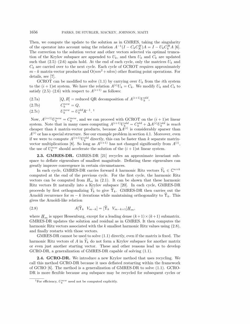
We study a sequence of linear systems taken from a finite element code developedby Philippe Geubelle and Spandan Maiti (both Aerospace Engineering, Universityof Illinois at Urbana-Champaign (UIUC)). In our example, the code simulates crackpropagation in a metal plate using so-called cohesive finite elements. The plate meshis shown in Figure 4.1. The problem is symmetric about the x-axis, and the crackpropagates exactly along this symmetry axis. The cohesive elements act as nonlinearsprings connecting the surfaces that will define the crack location. As the crack prop-agates, the cohesive elements deform following a nonlinear yield curve and eventuallybreak. The element stiffness is set to zero for a broken cohesive element. These ele-ments are usually inserted dynamically, but that is not the case here. This simulationresults in a sequence of sparse, symmetric, positive definite stiffness matrices thatchange slowly from one system to the next. Each stiffness matrix can be expressedas A(i+1) = A(i) + ΔA(i). Although ΔA(i) is considerably more sparse than A(i), itis not low-rank, as the terms in the update ΔA(i) come from all nonbroken cohesiveelements. The other finite elements model linear elasticity and have constant stiffnessmatrices. The matrices produced in our examples are 3988 × 3988, and have a con-dition number on the order of 104 before preconditioning. They have an average of13.4 nonzero entries per row. Over 2000 linear systems must be solved to capture thefracture progression.


Fig. 4.1. Two-dimensional plate mesh for the crack propagation problem.

150

200

250

300

350

400

450

500

550

400 420 440 460 480 500 520 540

Num

ber

of M

atrix

-Vec

tor

Pro

duct

s

Timestep (problem index)

CGGMRES(∞)

GCROT(40,29,25,7,1,2)

GMRES-DR(40,20)GCRO-DR(40,20) (Recycle)

GCROT(40,29,25,7,1,2) (Recycle)

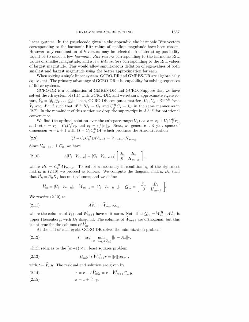
Fig. 4.2. Number of matrix-vector products versus timestep for various solvers for the crackpropagation problem without preconditioning. All solvers use a recurrence of at most 40 vectors,except GMRES(∞) and CG.

We examine the 151 linear systems 400–550, representing a typical subset ofthe fracture progression in which many cohesive elements break. We start with astraightforward comparison of GCRO-DR and GCROT with subspace recycling withCG, restarted GMRES, GMRES(∞), GMRES-DR, and GCROT without subspacerecycling. We always start with a zero initial guess, since we solve for the incrementaldisplacement associated with the loading increment. We give both preconditioned andnonpreconditioned convergence results. All solvers are required to reduce the relativeresidual to 1.0 × 10−10. In Figure 4.2 we give the number of matrix-vector productsneeded to solve each of these systems without preconditioning for GMRES(∞), CG,GMRES-DR(40,20), GCRO-DR(40,20), and GCROT(40,34,30,5,1,2), both with andwithout subspace recycling. Except for GMRES(∞) and CG, all methods in Figure 4.2minimize over a subspace of dimension 40 in each cycle. GMRES(40) is not shown,because it required too many matrix-vector products. In Figure 4.3 we give results forthe same sequence of problems and the same methods but with incomplete Cholesky(IC(0)) preconditioning. A new preconditioner was computed for each matrix, whichis not the most efficient approach. The total number of matrix-vector products neededto solve all 151 preconditioned linear systems is given in Table 4.1.


40

50

60

70

80

90

100

400 420 440 460 480 500 520 540

Num

ber

of M

atrix

-Vec

tor

Pro

duct

s


CGGMRES(∞)

GCROT(40,29,25,7,1,2)

GMRES-DR(40,20)GCRO-DR(40,20) (Recycle)

GCROT(40,29,25,7,1,2) (Recycle)

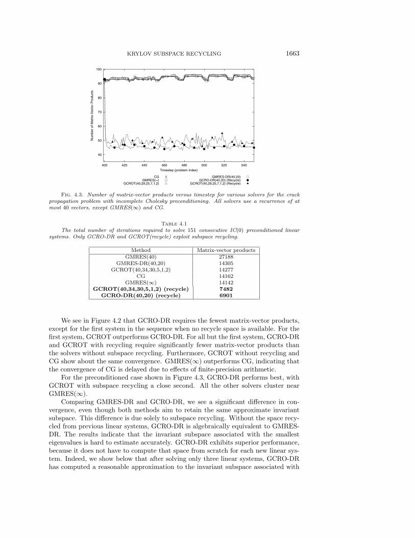
Fig. 4.3. Number of matrix-vector products versus timestep for various solvers for the crackpropagation problem with incomplete Cholesky preconditioning. All solvers use a recurrence of atmost 40 vectors, except GMRES(∞) and CG.

Table 4.1

The total number of iterations required to solve 151 consecutive IC(0) preconditioned linearsystems. Only GCRO-DR and GCROT(recycle) exploit subspace recycling.

Method Matrix-vector productsGMRES(40) 27188

GMRES-DR(40,20) 14305GCROT(40,34,30,5,1,2) 14277

CG 14162GMRES(∞) 14142

GCROT(40,34,30,5,1,2) (recycle) 7482GCRO-DR(40,20) (recycle) 6901

We see in Figure 4.2 that GCRO-DR requires the fewest matrix-vector products,except for the first system in the sequence when no recycle space is available. For thefirst system, GCROT outperforms GCRO-DR. For all but the first system, GCRO-DRand GCROT with recycling require significantly fewer matrix-vector products thanthe solvers without subspace recycling. Furthermore, GCROT without recycling andCG show about the same convergence. GMRES(∞) outperforms CG, indicating thatthe convergence of CG is delayed due to effects of finite-precision arithmetic.

For the preconditioned case shown in Figure 4.3, GCRO-DR performs best, withGCROT with subspace recycling a close second. All the other solvers cluster nearGMRES(∞).

Comparing GMRES-DR and GCRO-DR, we see a significant difference in con-vergence, even though both methods aim to retain the same approximate invariantsubspace. This difference is due solely to subspace recycling. Without the space recy-cled from previous linear systems, GCRO-DR is algebraically equivalent to GMRES-DR. The results indicate that the invariant subspace associated with the smallesteigenvalues is hard to estimate accurately. GCRO-DR exhibits superior performance,because it does not have to compute that space from scratch for each new linear sys-tem. Indeed, we show below that after solving only three linear systems, GCRO-DRhas computed a reasonable approximation to the invariant subspace associated with


-10

-8

-6

-4

-2

0

0 50 100 150 200 250 300 350 400 450

log 1

0 ||r

|| 2

Number of Matrix-Vector Products

GCRO-DRGMRES(∞)

Bound from Theorem 3.1

Fig. 4.4. Convergence curves for GCRO-DR on five consecutive linear systems from the pre-conditioned crack propagation problem, along with the bound described in Theorem 3.1. The boundwas computed with Q the eigenspace corresponding to the 20 smallest eigenvalues of the precondi-tioned operator. Since the bound is tight and δ is small, GCRO-DR achieved the convergence rateof the deflated problem in Theorem 3.1.

Table 4.2

Table of δ (Q, C) for GCRO-DR(40, 20) on the preconditioned crack propagation problem, whereQ has been selected as the invariant subspace associated with the 15 eigenvalues of smallest mag-nitude. The decrease of δ within a column indicates the improvement of the approximation to Qfor a particular system. The small perturbation of the invariant subspace is reflected in the minorincrease in δ from the last cycle of one system to before the first of the next system. At each cycle,GCRO-DR updates its approximate invariant subspace.

Linear system 401 402 403 404 405

Before cycle 1 0.9994 0.2380 0.0464 0.0607 0.0794After cycle 1 0.9180 0.1448 0.0463 0.0606 0.0787After cycle 2 0.2446 0.0302 0.0416 0.0568 0.0690After cycle 3 0.2331 0.0302 0.0415 0.0567 0.0684

the fifteen smallest eigenvalues; GMRES-DR cannot do this.Next, we evaluate some of the properties of GCRO-DR related to the two theo-

retical results in section 3 and the three properties mentioned in the introduction.As GCRO-DR approximates an invariant subspace better, it gets closer to the

convergence rate of a deflated problem, as described in Theorem 3.1. The conver-gence curves for five consecutive systems from the preconditioned crack propagationproblem are shown in Figure 4.4, along with the bound described in Theorem 3.1.The bound was computed with the invariant subspace, Q, corresponding to the 20smallest eigenvalues of the preconditioned matrix. We see that the bound is sharp.Additionally, note that for each problem the initial convergence rate for GCRO-DRis approximately the same as the final convergence rate of GMRES(∞).

In Table 4.2, for the preconditioned example we show how the one-sided distanceδ, defined in (3.1), from the invariant subspace associated with the 15 smallest eigen-values to the recycle space evolves over multiple cycles and multiple linear systems.This table illustrates a number of important issues.

The first system solved in this experiment is system 400, and so system 401 is thefirst system that starts with a recycle space. For the chosen invariant subspace δ is


quite poor at the start, but δ improves quickly over the next two linear systems, andafter cycle 2 for system 402, δ has taken a reasonably small value. So, GCRO-DR isable to compute from scratch increasingly good approximations to invariant subspacesthat change slightly from system to system. Note that GMRES-DR starts from scratchfor every new system. Therefore, it never obtains a sufficiently good approximation,and hence requires many additional iterations per linear system. Any other methodthat cannot continually update the approximation to the invariant subspace will sufferfrom the same problem.

Next, note how δ improves during the solution of a single linear system, whereasthe small perturbation of the invariant subspace for the next linear system is reflectedin the minor increase in δ from the last cycle of one system to before the first cycleof the next system. This confirms our earlier statement, based on Theorem 3.2, thatthe invariant subspace associated with the smallest eigenvalues and smooth globalmodes changes little under small local changes in the model. We have also verified thisexplicitly by computing the principal angles between invariant subspaces of successivematrices. However, in the next experiment we show that the cumulative change overa larger number of loading steps requires the continual or at least periodic updatingof the recycle space to keep the number of iterations small.

Finally, this particular Q was chosen to illustrate the role and behavior of δ, notto get the best bound from Theorem 3.1. Initially, a smaller invariant subspace mighthave a much smaller δ and may lead to a tighter bound. The bound holds for anyinvariant subspace with δ < 1, and so the smallest bound is the effective one.

Next, we provide a number of experiments that illustrate how quickly GCRO-DRand GCROT learn and adapt to an updated linear system, and how the convergencerate deteriorates if we stop updating the recycle space.

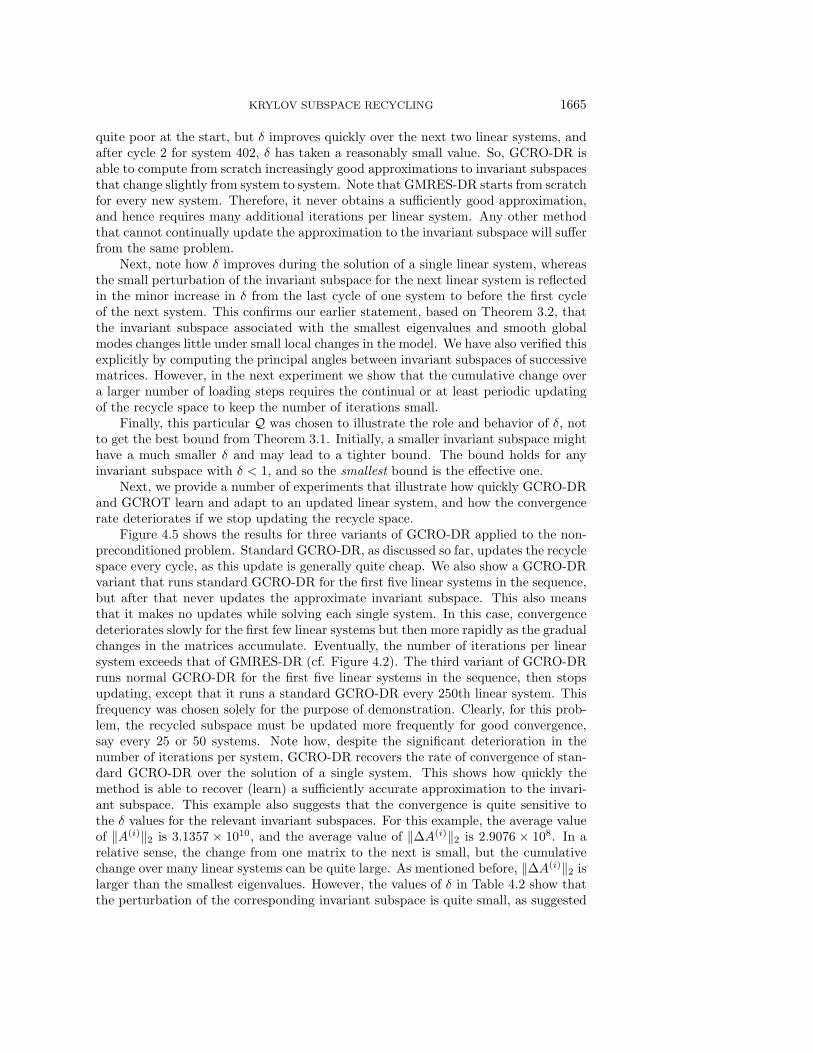
Figure 4.5 shows the results for three variants of GCRO-DR applied to the non-preconditioned problem. Standard GCRO-DR, as discussed so far, updates the recyclespace every cycle, as this update is generally quite cheap. We also show a GCRO-DRvariant that runs standard GCRO-DR for the first five linear systems in the sequence,but after that never updates the approximate invariant subspace. This also meansthat it makes no updates while solving each single system. In this case, convergencedeteriorates slowly for the first few linear systems but then more rapidly as the gradualchanges in the matrices accumulate. Eventually, the number of iterations per linearsystem exceeds that of GMRES-DR (cf. Figure 4.2). The third variant of GCRO-DRruns normal GCRO-DR for the first five linear systems in the sequence, then stopsupdating, except that it runs a standard GCRO-DR every 250th linear system. Thisfrequency was chosen solely for the purpose of demonstration. Clearly, for this prob-lem, the recycled subspace must be updated more frequently for good convergence,say every 25 or 50 systems. Note how, despite the significant deterioration in thenumber of iterations per system, GCRO-DR recovers the rate of convergence of stan-dard GCRO-DR over the solution of a single system. This shows how quickly themethod is able to recover (learn) a sufficiently accurate approximation to the invari-ant subspace. This example also suggests that the convergence is quite sensitive tothe δ values for the relevant invariant subspaces. For this example, the average valueof ‖A(i)‖2 is 3.1357 × 1010, and the average value of ‖ΔA(i)‖2 is 2.9076 × 108. In arelative sense, the change from one matrix to the next is small, but the cumulativechange over many linear systems can be quite large. As mentioned before, ‖ΔA(i)‖2 islarger than the smallest eigenvalues. However, the values of δ in Table 4.2 show thatthe perturbation of the corresponding invariant subspace is quite small, as suggested


200

300

400

500

600

700

800

900

400 500 600 700 800 900 1000

Num

ber

of M

atrix

-Vec

tor

Pro

duct

s


GCRO-DR(40,20) (Recycle)GCRO-DR(40,20) (Stop updating after system 405)

GCRO-DR(40,20) (Update every 250 systems)

Fig. 4.5. Number of matrix-vector products versus timestep for GCRO-DR(40, 20) with subspacerecycling on the nonpreconditioned crack propagation problem. We also show a modified version ofGCRO-DR(40, 20) that stops updating the recycled subspace after linear system 405, and a versionthat stops updating after linear system 405 but does update every 250 systems thereafter. Convergencequickly deteriorates in the latter two cases, showing the importance of updating the approximateinvariant subspace regularly.

by the discussion in section 3 regarding small localized changes in the problem andby Theorem 3.2. Figure 4.5 shows that GCRO-DR can adapt to the slow change ofthe invariant subspace. Finally, it would not be hard to dynamically balance the costof updating the recycle space with the improved rate of convergence.

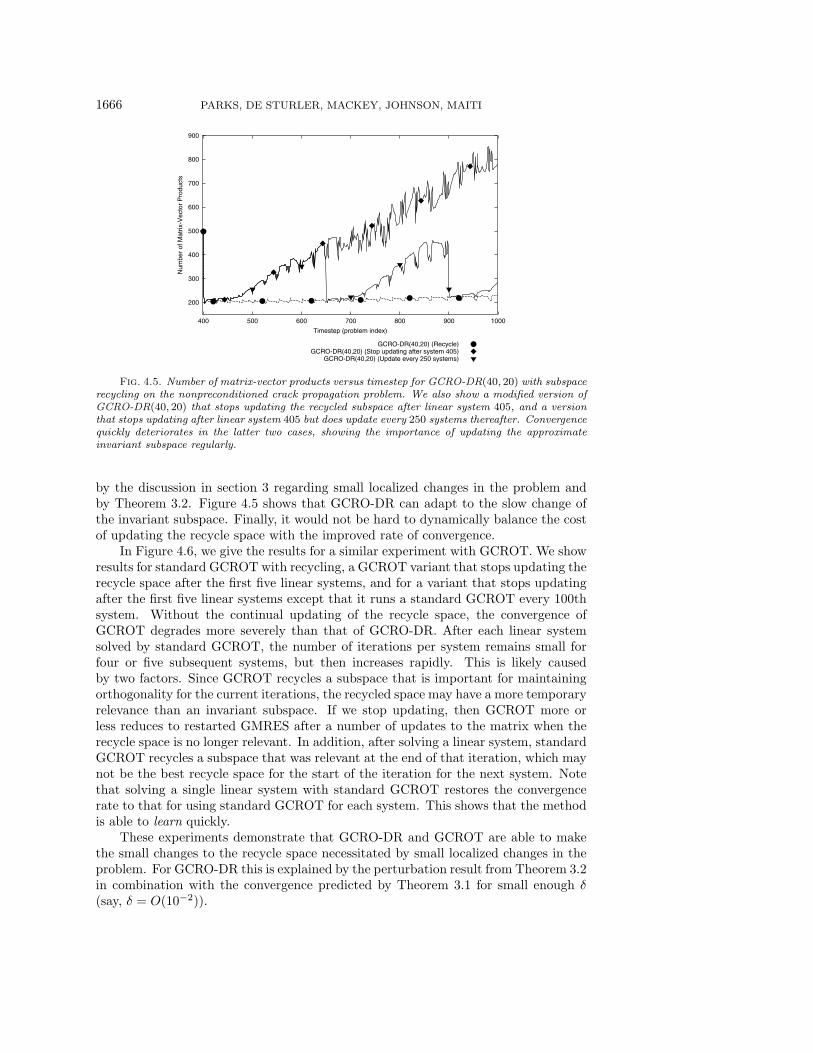
In Figure 4.6, we give the results for a similar experiment with GCROT. We showresults for standard GCROT with recycling, a GCROT variant that stops updating therecycle space after the first five linear systems, and for a variant that stops updatingafter the first five linear systems except that it runs a standard GCROT every 100thsystem. Without the continual updating of the recycle space, the convergence ofGCROT degrades more severely than that of GCRO-DR. After each linear systemsolved by standard GCROT, the number of iterations per system remains small forfour or five subsequent systems, but then increases rapidly. This is likely causedby two factors. Since GCROT recycles a subspace that is important for maintainingorthogonality for the current iterations, the recycled space may have a more temporaryrelevance than an invariant subspace. If we stop updating, then GCROT more orless reduces to restarted GMRES after a number of updates to the matrix when therecycle space is no longer relevant. In addition, after solving a linear system, standardGCROT recycles a subspace that was relevant at the end of that iteration, which maynot be the best recycle space for the start of the iteration for the next system. Notethat solving a single linear system with standard GCROT restores the convergencerate to that for using standard GCROT for each system. This shows that the methodis able to learn quickly.

These experiments demonstrate that GCRO-DR and GCROT are able to makethe small changes to the recycle space necessitated by small localized changes in theproblem. For GCRO-DR this is explained by the perturbation result from Theorem 3.2in combination with the convergence predicted by Theorem 3.1 for small enough δ(say, δ = O(10−2)).


200

400

600

800

1000

1200

1400

400 500 600 700 800 900 1000

Num

ber

of M

atrix

-Vec

tor

Pro

duct

s


GCROT(40,29,25,7,1,2) (Recycle)GCROT(40,29,25,7,1,2) (Stop updating after system 405)

GCROT(40,29,25,7,1,2) (Update every 100 systems)

Fig. 4.6. Number of matrix-vector products versus timestep for GCROT(40, 29, 25, 7, 1, 2) withsubspace recycling on the nonpreconditioned crack propagation problem. We also show a modifiedversion of GCROT(40, 29, 25, 7, 1, 2) that stops updating the recycled subspace after linear system405, and a version that stops updating after linear system 405 but runs standard GCROT every100th system thereafter. In the latter case, convergence remains small for about four or five systemsafter using standard GCROT, but then quickly deteriorates, showing the importance of updating theapproximate invariant subspace regularly. Note that GCROT, too, is able to restore rapid conver-gence in the course of a single linear system.

4.2. Electronic structure. First-principles, electronic-structure calculationsbased on the Schrodinger equation are used to predict key physical properties ofmaterials systems with a large number of atoms. We consider systems arising in theKKR (Korringa–Kohn–Rostoker) method [16, 17] and seek to compute entries in theinverse of the matrix

G = (I − (t− tref)Gref)−1(t− tref),

where Gref is a sparse and easily invertible matrix and t and tref are block-diagonalmatrices. G is a sparse, complex, non-Hermitian matrix whose relative number ofnonzeros decreases with the number of atoms [14, 40, 32].

Only the block-diagonal elements of G−1 are needed to calculate physical proper-ties, such as charge densities, total energy, force, and formation and defect energies.As such, we solve GX = I, column-by-column. Iterative methods offer the advan-tage of storing only those components of the inverse that we need. Standard directinversion methods are infeasible for large numbers of atoms (N ≥ 500) on regu-lar workstations, because the memory and computational costs grow as O(N2) andO(N3), respectively.

We consider a small model problem provided by Duane Johnson (Materials Sci-ence and Engineering, UIUC) and Andrei Smirnov (Oak Ridge National Laboratory).The problem involves the simulation of a cubic lattice of 54 copper atoms (treated asinequivalent) for a complex energy point close to the real axis. This is the key physicalregime for metals and leads to problems that converge poorly. The matrix is 864×864and has about 300,000 nonzeros. However, for increasingly larger systems the matrix


-10

-8

-6

-4

-2

0

0 500 1000 1500 2000 2500

log 1

0 ||r

|| 2

Total Number of Matrix-Vector Products

Fig. 4.7. Convergence for 16 consecutive right-hand sides for a small electronic structureproblem. Each distinct curve gives the convergence for a subsequent right-hand side, plotted againstthe total number of matrix-vector products. The first two right-hand sides together take about 500iterations, while the remaining right-hand sides take about 140 iterations each, a reduction of almost50%.

becomes more sparse; the number of nonzeros grows roughly linearly with the size ofthe matrix. We solved this problem using GCRO-DR(50,25) with subspace recyclingfor 32 consecutive right-hand sides (the first 32 unit Cartesian basis vectors). Wegive the convergence history for the first atom in Figure 4.7. Note that the first tworight-hand sides together take about 500 iterations; the remaining right-hand sidestake approximately 140 iterations each, a reduction of almost 50%. Each right-handside for the second atom (not shown) also takes approximately 140 iterations. Al-though for problems of this size iterative methods are not competitive with directsolvers, we have observed this convergence behavior for larger problems, in particularthe immediate acceleration in convergence for subsequent right-hand sides.

4.3. QCD. Quantum chromodynamics (QCD) is the fundamental theory de-scribing the strong interaction between quarks and gluons. Numerical simulations ofQCD on a four-dimensional space-time lattice are considered the only way to solveQCD ab initio [4, 35]. As the problem has a 12 × 12 block structure, we are ofteninterested in solving for 12 right-hand sides related to a single lattice site. The linearsystem to be solved is (I − κD)x = b with 0 ≤ κ < κc, where D is a sparse, complex,non-Hermitian matrix representing periodic nearest neighbor coupling on the four-dimensional space-time lattice [19]. For κ = κc the system becomes singular. Thephysically interesting case is for κ slightly smaller than κc; κc depends on D.

As a model problem we use the matrix conf5.0 00l4x4.1000.mtx downloadedfrom the Matrix Market website at NIST [2]. The model problems were submitted byMedeke [19]. For this problem we have κc = 0.20611, and we used κ = 0.202.

We solve for 12 consecutive right-hand sides (the first 12 Cartesian basis vectors)using the GCROT method with subspace recycling. The results are presented inFigure 4.8.


-10

-8

-6

-4

-2

0

0 500 1000 1500 2000 2500

log 1

0 ||r

|| 2

Total Number of Matrix-Vector Products

Fig. 4.8. Convergence for 12 consecutive right-hand sides for a model QCD problem from theNIST Matrix Market. Each distinct curve gives the convergence for a subsequent right-hand side,plotted against the total number of matrix-vector products. Note that the final convergence rate forthe first system is the starting convergence rate for the rest of the systems.

4.4. Convection-diffusion. We consider the finite difference discretization ofthe partial differential equation

uxx + uyy + cux = 0

on (0, 1) × (0, 1) with boundary conditions

u(x, 0) = u(0, y) = 0,

u(x, 1) = u(1, y) = 1.

Central differences are used, and we set the mesh width to be h = 1/41 in bothdirections, which results in a 1600 × 1600 matrix. We consider the symmetric case,c = 0, and a nonsymmetric case for c = 40. The eigenvalues are real for both theseexamples. In order to study how a recycled subspace affects convergence, we willconsider the “ideal” situation for subspace recycling by solving a linear system twicewith GCRO-DR and GCROT, recycling the subspace generated from the first run.

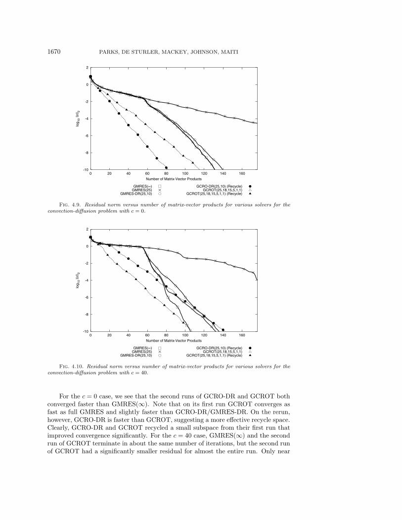
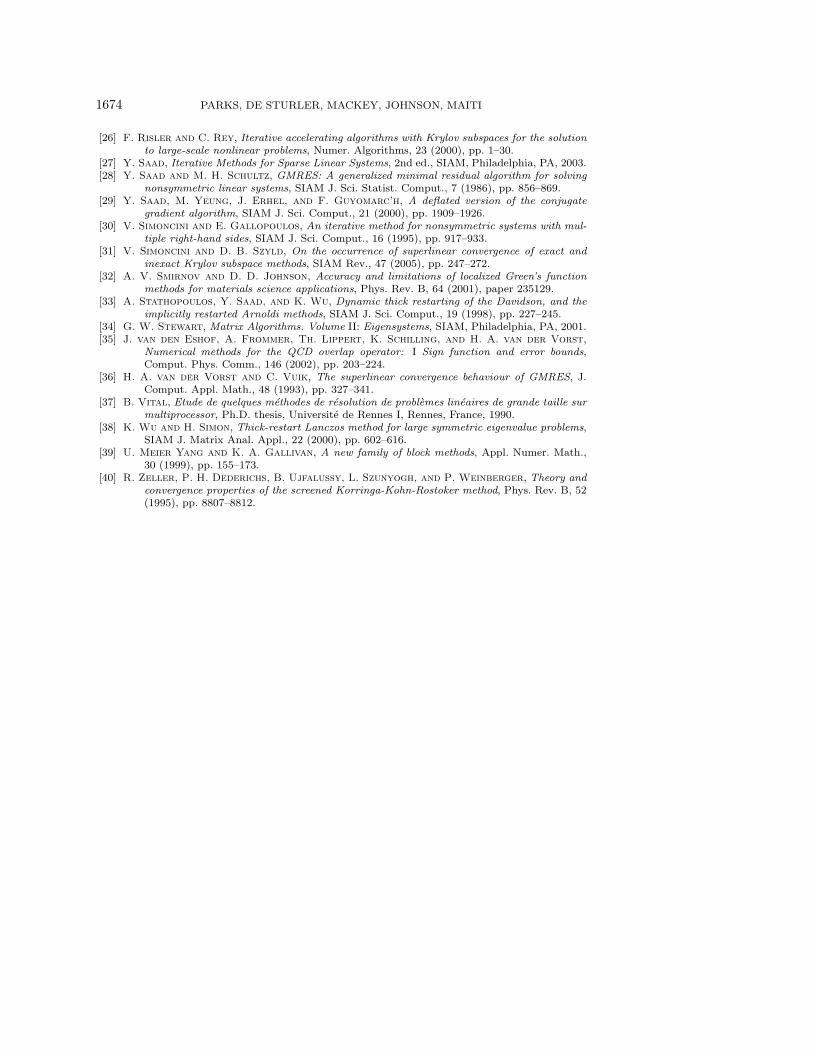
In this example, we consider GMRES(∞), GMRES(25), GMRES-DR(25,10),GCRO-DR(25,10), and GCROT(25,18,15,5,1,1). To explore the effects of subspacerecycling on this example problem, we rerun GCRO-DR and GCROT on the samelinear system, and recycle the subspace from the first run. We do this to exclude theeffects of right-hand sides having slightly different eigenvector decompositions. In asense, this is the ideal case for subspace recycling. The first run for GCRO-DR isthe same as GMRES-DR. The results for the c = 40 (nonsymmetric) case are quiteinteresting and counterintuitive. In particular, this example suggests that there arebetter choices for a recycle space than approximate invariant subspaces. This topicis discussed further in [23]. We give the results for the symmetric case, c = 0, inFigure 4.9 and for the nonsymmetric case with c = 40 in Figure 4.10. In the legendfor each of these figures, Recycle denotes the second run of a solver that was run twice.All solvers were required to reduce the relative residual to 1.0 × 10−10.


-10

-8

-6

-4

-2

0

2

0 20 40 60 80 100 120 140 160

log 1

0 ||r

|| 2


GMRES(∞)GMRES(25)

GMRES-DR(25,10)

GCRO-DR(25,10) (Recycle)GCROT(25,18,15,5,1,1)

GCROT(25,18,15,5,1,1) (Recycle)

Fig. 4.9. Residual norm versus number of matrix-vector products for various solvers for theconvection-diffusion problem with c = 0.

-10

-8

-6

-4

-2

0

2

0 20 40 60 80 100 120 140 160

log 1

0 ||r

|| 2


GMRES(∞)GMRES(25)

GMRES-DR(25,10)

GCRO-DR(25,10) (Recycle)GCROT(25,18,15,5,1,1)

GCROT(25,18,15,5,1,1) (Recycle)

Fig. 4.10. Residual norm versus number of matrix-vector products for various solvers for theconvection-diffusion problem with c = 40.

For the c = 0 case, we see that the second runs of GCRO-DR and GCROT bothconverged faster than GMRES(∞). Note that on its first run GCROT converges asfast as full GMRES and slightly faster than GCRO-DR/GMRES-DR. On the rerun,however, GCRO-DR is faster than GCROT, suggesting a more effective recycle space.Clearly, GCRO-DR and GCROT recycled a small subspace from their first run thatimproved convergence significantly. For the c = 40 case, GMRES(∞) and the secondrun of GCROT terminate in about the same number of iterations, but the second runof GCROT had a significantly smaller residual for almost the entire run. Only near


Table 4.3

Cosines of principal angles between the recycled subspace and the invariant subspaces spannedby the 10 and 21 eigenvectors associated with the eigenvalues of smallest magnitude, respectively,for the c = 0 and c = 40 cases.

Cosines of principal angles between recycledsubspace and subspace associated with 10smallest magnitude eigenvalues

Cosines of principal angles between recycledsubspace and subspace associated with 21smallest magnitude eigenvalues

c = 0 c = 40 c = 0 c = 401.00000000000000 1.00000000000000 1.00000000000000 1.000000000000001.00000000000000 0.99999999999997 1.00000000000000 1.000000000000001.00000000000000 0.99999999839942 1.00000000000000 1.000000000000001.00000000000000 0.99999970490203 1.00000000000000 0.999999999999370.99999999999703 0.99990149788562 1.00000000000000 0.999999995453940.00000000593309 0.98844658524616 1.00000000000000 0.999996810645650.00000000003840 0.89957454665058 0.99999999999988 0.999838960062150.00000000000003 0.54237185670110 0.99999999316379 0.993930079435470.00000000000000 0.06426938073642 0.99993817690380 0.945845199764710.00000000000000 0.02603228754605 0.99792215267787 0.20867650942988

the end, with a much larger search space, does GMRES(∞) catch up. The second runof GCROT also does better than its first run, indicating that it recycled a subspaceuseful for convergence. However, GCRO-DR performed initially somewhat betteron the second run than the first, but the overall iteration count was approximatelythe same for both runs. This means that the subspace it recycled failed to improveconvergence. For more analysis on the selection of good recycle spaces, see [23, 15, 24].

Table 4.3 shows the cosines of the principal angles between the subspace recycledby GCRO-DR and the invariant subspaces associated with the 10 and 21 eigenvaluesof smallest magnitude, respectively, for the c = 0 and c = 40 cases. For the comparisonwith 10 eigenvectors, we see that the recycle space for the c = 0 case captures only5 eigenvectors. We compare with the space spanned by 21 eigenvectors because itcaptures the entire recycled subspace for the c = 0 case. This means that GCRO-DRdoes not select the invariant subspace spanned by the eigenvectors for the 10 smallesteigenvalues, but rather selects some subspace of the space spanned by the 21 smallest.The table also shows that the approximation of an invariant subspace for the c = 40case is nearly as good as for c = 0. However, this does not lead to similar convergence.

5. Conclusions and future work. We have presented an overview of Krylovsubspace recycling for sequences of linear systems, where both the matrix and right-hand side change. Different choices for subspace selection and recycling have beenshown, as well as methods implementing those choices. We propose the new solverGCRO-DR to implement Krylov subspace recycling of approximate invariant sub-spaces for Hermitian and non-Hermitian systems. We provide two important theo-retical results complemented by a set of experiments to analyze the convergence ofGCRO-DR for a typical application generating a long sequence of linear systems.GCROT has convergence behavior similar to GCRO-DR regarding recycling, buttheoretical results for this method are a topic of future research. When solving asequence of linear systems, methods employing Krylov subspace recycling frequentlyoutperformed GMRES(∞) while recycling a subspace of only small dimension andminimizing over a small subspace. However, as particular examples in section 4.4show, it is not completely clear how subspace selection affects convergence, so fur-ther theory is needed. Short recurrence methods for the Hermitian case have beendeveloped [15].


Appendix. GCRO with deflated restarting (GCRO-DR).

1: Choose m, the maximum size of the subspace, and k, the desired number of

approximate eigenvectors. Let tol be the convergence tolerance. Choose an initial

guess x0. Compute r0 = b−Ax0, and set i = 1.

2: if Yk is defined (from solving a previous linear system) then

3: Let [Q,R] be the reduced QR-factorization of AYk.

4: Ck = Q

5: Uk = YkR−1

6: x1 = x0 + UkCHk r0

7: r1 = r0 − CkCHk r0

8: else

9: v1 = r0/‖r0‖2

10: c = ‖r0‖2e1

11: Perform m steps of GMRES, solving min ‖c−Hmy‖2 for y and generating Vm+1

and Hm.

12: x1 = x0 + Vmy

13: r1 = Vm+1(c−Hmy)

14: Compute the k eigenvectors zj of (Hm+h2m+1,mH−H

m emeHm)zj = θj zj associated

with the smallest magnitude eigenvalues θj and store in Pk.

15: Yk = VmPk

16: Let [Q,R] be the reduced QR-factorization of HmPk.

17: Ck = Vm+1Q

18: Uk = YkR−1

19: end if

20: while ‖ri‖2 > tol do

21: i = i + 1

22: Perform m − k Arnoldi steps with the linear operator (I − CkCHk )A, letting

v1 = ri−1/‖ri−1‖2 and generating Vm−k+1, Hm−k, and Bm−k.

23: Let Dk be a diagonal scaling matrix such that Uk = UkDk, where the columns

of Uk have unit norm.

24: Vm = [Uk Vm−k]

25: Wm+1 = [Ck Vm−k+1]

26: Gm =

[Dk Bm−k

0 Hm−k

]27: Solve min ‖WH

m+1ri−1 −Gmy‖2 for y.

28: xi = xi−1 + Vmy

29: ri = ri−1 − Wm+1Gmy

30: Compute the k eigenvectors zi of GHmGmzi = θiG

HmWH

m+1Vmzi associated with

smallest magnitude eigenvalues θi and store in Pk.

31: Yk = VmPk

32: Let [Q,R] be the reduced QR-factorization of GmPk.

33: Ck = Wm+1Q

34: Uk = YkR−1

35: end while

36: Let Yk = Uk (for the next system).


Acknowledgments. We thank one of the anonymous referees and the editor fortheir helpful comments and for making some very useful suggestions regarding theexperimental analysis.

REFERENCES

[1] C. Beattie, M. Embree, and J. Rossi, Convergence of restarted Krylov subspaces to invariantsubspaces, SIAM J. Matrix Anal. Appl., 25 (2004), pp. 1074–1109.

[2] R. F. Boisvert, R. Pozo, K. Remington, R. F. Barrett, and J. J. Dongarra, Matrixmarket: A Web resource for test matrix collections, in Quality of Numerical Software:Assessment and Enhancement, Ronald F. Boisvert, ed., Chapman and Hall, London, 1997,pp. 125–136.

[3] T. F. Chan and M. K. Ng, Galerkin projection methods for solving multiple linear systems,SIAM J. Sci. Comput., 21 (1999), pp. 836–850.

[4] M. Creutz, Quarks, Gluons, and Lattices, Cambridge University Press, Cambridge, UK, 1986.[5] E. de Sturler, Inner-outer methods with deflation for linear systems with multiple right-hand

sides, in Householder Symposium XIII, Proceedings of the Householder Symposium onNumerical Algebra, 1996, pp. 193–196.

[6] E. de Sturler, Nested Krylov methods based on GCR, J. Comput. Appl. Math., 67 (1996),pp. 15–41.

[7] E. de Sturler, Truncation strategies for optimal Krylov subspace methods, SIAM J. Numer.Anal., 36 (1999), pp. 864–889.

[8] J. J. Dongarra, I. S. Duff, D. C. Sorensen, and H. A. van der Vorst, Numerical LinearAlgebra for High-Performance Computers, Software Environ. Tools 7, SIAM, Philadelphia,PA, 1998.

[9] M. Eiermann, O. G. Ernst, and O. Schneider, Analysis of acceleration strategies forrestarted minimal residual methods, J. Comput. Appl. Math., 123 (2000), pp. 261–292.

[10] C. Farhat and F.-X. Roux, Implicit parallel processing in structural mechanics, in Com-putational Mechanics Advances, J. Tinsley Oden, ed., North–Holland, Amsterdam, 1994,Vol. 2, pp. 1–124.

[11] P. F. Fischer, Projection techniques for iterative solution of Ax = b with successive right-handsides, Comput. Methods Appl. Mech. Engrg., 163 (1998), pp. 193–204.

[12] G. H. Golub and C. F. Van Loan, Matrix Computations, 3rd ed., Johns Hopkins UniversityPress, Baltimore, MD, 1996.

[13] A. Gullerud and R. H. Dodds, MPI-based implementation of a PCG solver using an EBEarchitecture and preconditioner for implicit, 3-D finite element analyses, Comput. & Struc-tures, 79 (2001), pp. 553–575.

[14] D. D. Johnson, D. M. Nicholson, F. J. Pinski, B. L. Gyorffy, and G. M. Stocks, En-ergy and pressure calculations for random substitutional alloys, Phys. Rev. B, 41 (1990),pp. 9701–9716.

[15] M. E. Kilmer and E. de Sturler, Recycling subspace information for diffuse optical tomog-raphy, SIAM J. Sci. Comput., 27 (2006), pp. 2140–2166.

[16] W. Kohn and N. Rostoker, Solution of the Schrodinger equation in periodic lattices with anapplication to metallic lithium, Phys. Rev., 94 (1954), pp. 1111–1120.

[17] J. Korringa, On the calculation of the energy of a Bloch wave in a metal, Phys., 8 (1947),pp. 392–400.

[18] G. Mackey, Reusing Krylov Subspaces for Sequences of Linear Systems, Master’s thesis, De-partment of Computer Science, University of Illinois at Urbana-Champaign, 2003.

[19] B. Medeke, Set QCD: Quantum Chromodynamics, description of matrix set on NIST MatrixMarket, http://math.nist.gov/MatrixMarket.

[20] R. B. Morgan, Implicitly restarted GMRES and Arnoldi methods for nonsymmetric systemsof equations, SIAM J. Matrix Anal. Appl., 21 (2000), pp. 1112–1135.

[21] R. B. Morgan, GMRES with deflated restarting, SIAM J. Sci. Comput., 24 (2002), pp. 20–37.[22] D. P. O’Leary, The block conjugate gradient algorithm and related methods, Linear Algebra

Appl., 29 (1980), pp. 293–322.[23] M. L. Parks, The Iterative Solution of a Sequence of Linear Systems Arising from Nonlinear

Finite Element Analysis, Ph.D. thesis, Department of Computer Science, University ofIllinois at Urbana-Champaign, 2005.

[24] M. L. Parks and E. de Sturler, Analysis of Krylov subspace recycling for sequences of linearsystems, 2006, to appear.

[25] C. Rey and F. Risler, A Rayleigh-Ritz preconditioner for the iterative solution to large-scalenonlinear problems, Numer. Algorithms, 17 (1998), pp. 279–311.


[26] F. Risler and C. Rey, Iterative accelerating algorithms with Krylov subspaces for the solutionto large-scale nonlinear problems, Numer. Algorithms, 23 (2000), pp. 1–30.

[27] Y. Saad, Iterative Methods for Sparse Linear Systems, 2nd ed., SIAM, Philadelphia, PA, 2003.[28] Y. Saad and M. H. Schultz, GMRES: A generalized minimal residual algorithm for solving

nonsymmetric linear systems, SIAM J. Sci. Statist. Comput., 7 (1986), pp. 856–869.[29] Y. Saad, M. Yeung, J. Erhel, and F. Guyomarc’h, A deflated version of the conjugate

gradient algorithm, SIAM J. Sci. Comput., 21 (2000), pp. 1909–1926.[30] V. Simoncini and E. Gallopoulos, An iterative method for nonsymmetric systems with mul-

tiple right-hand sides, SIAM J. Sci. Comput., 16 (1995), pp. 917–933.[31] V. Simoncini and D. B. Szyld, On the occurrence of superlinear convergence of exact and

inexact Krylov subspace methods, SIAM Rev., 47 (2005), pp. 247–272.[32] A. V. Smirnov and D. D. Johnson, Accuracy and limitations of localized Green’s function

methods for materials science applications, Phys. Rev. B, 64 (2001), paper 235129.[33] A. Stathopoulos, Y. Saad, and K. Wu, Dynamic thick restarting of the Davidson, and the

implicitly restarted Arnoldi methods, SIAM J. Sci. Comput., 19 (1998), pp. 227–245.[34] G. W. Stewart, Matrix Algorithms. Volume II: Eigensystems, SIAM, Philadelphia, PA, 2001.[35] J. van den Eshof, A. Frommer, Th. Lippert, K. Schilling, and H. A. van der Vorst,

Numerical methods for the QCD overlap operator: I Sign function and error bounds,Comput. Phys. Comm., 146 (2002), pp. 203–224.

[36] H. A. van der Vorst and C. Vuik, The superlinear convergence behaviour of GMRES, J.Comput. Appl. Math., 48 (1993), pp. 327–341.

[37] B. Vital, Etude de quelques methodes de resolution de problemes lineaires de grande taille surmultiprocessor, Ph.D. thesis, Universite de Rennes I, Rennes, France, 1990.

[38] K. Wu and H. Simon, Thick-restart Lanczos method for large symmetric eigenvalue problems,SIAM J. Matrix Anal. Appl., 22 (2000), pp. 602–616.

[39] U. Meier Yang and K. A. Gallivan, A new family of block methods, Appl. Numer. Math.,30 (1999), pp. 155–173.

[40] R. Zeller, P. H. Dederichs, B. Ujfalussy, L. Szunyogh, and P. Weinberger, Theory andconvergence properties of the screened Korringa-Kohn-Rostoker method, Phys. Rev. B, 52(1995), pp. 8807–8812.

recycling krylov subspaces for …mlparks/papers/krylovrecycling.pdfkrylov subspace recycling 1653...

Documents