AN ABSTRACT OF THE THESIS OF

Caleb Frederick Zurstadt for the degree of Master of Science in Fisheries Science presented on

March 7, 2000. Title: Relationships Between Relative Abundance of Resident Bull Trout(Salvelinus confluentus) and Habitat Characteristics in Central Idaho Mountain Streams.

Abstract approved:

William J. Liss

Resident bull trout (Salvelinus confluentus) may be particularly vulnerable to human related

disturbance, however very few studies have focused on resident bull trout populations. The

abundance of bull trout is one measure of the strength and potential for persistence of a

population. Habitat characteristics may influence resident bull trout abundance to differing

degrees and by varying means at multiple spatial scales. We used day and night snorkel

counts to assess relative bull trout abundance. A modification of the Forest Service Rl/R4

Fish and Fish Habitat Inventory was used to assess habitat characteristics associated with

resident bull trout. Logistic and multiple linear regression were used to assess the

relationships between resident bull trout abundance and habitat characteristics at the patch (1

to 5 km), reach (0.5 to 1 km) and habitat unit (1 to 100 m) scales. Site categorical variables

were used along with quantitative habitat variables to explain among-site and across-site

variation in the data. The significance of both quantitative habitat variables and categorical

site variables at various spatial scales suggest that relationships between bull trout abundance

and habitat characteristics are complex and in part dependent on scale. The characteristics of

individual habitat units explained little of the variation in bull trout presence/absence (logistic

regression; Somers' D = 0.44) and density (multiple linear regression; adjusted le = 0.08) in

habitat units, however there were habitat characteristics that were significantly (P 0.05)

correlated to bull trout presence/absence and density in habitat units. The relationships

Redacted for Privacy

between habitat characteristics and bull trout presence/absence and density varied between

habitat unit types. There was a strong quadratic relationship between bull trout abundance and

mean summer water temperature at the reach (P = 0.004) and patch scales (P = 0.001). The

mean temperature of patches appears to explain some of the variation in bull trout density at

smaller spatial scales, such as reaches and habitat units. An appreciation of the complex

nature of scale dependent interactions between bull trout abundance and habitat characteristics

may help resource managers make wiser decisions regarding conservation of resident bull

trout populations.

Relationships Between Relative Abundance of Resident Bull Trout (Salvelinus confluentus)and Habitat Characteristics in Central Idaho Mountain Streams

by

Caleb Frederick Zurstadt

A THESIS

submitted to

Oregon State University

in partial fulfillment ofthe requirements for the

degree of

Master of Science

Presented March 7, 2000Commencement June 2000

Master of Science in Fisheries Science thesis of Caleb Frederick Zurstadt presentedon March 7, 2000

APPROVED:

Major Pr , representing Fisheries Science

Head of DepartmtIlt/of Fisheries and Wildlife

Dean of e School

I understand that my thesis will become part of the permanent collection of Oregon StateUniversity libraries. My signature below authorizes release of my thesis to any readerupon request.

Caleb Frederick Zurstadt, Author

Redacted for Privacy

Redacted for Privacy

Redacted for Privacy

Redacted for Privacy

ACKNOWLEDGMENT

I would like to thank Kathy Golden, Mike Kaylor, Jay Lewellyn, Jenny Nyme, Duncan

Oswald, and Isaac Sanders for collecting monotonous habitat data and snorkeling in icy

streams, often groveling on hands and knees, during the day and at night. Without their

positive attitudes and hard work the data would never have been collected. The personnel of

the Lowman Ranger District provided the platform from which this project was carried out. I

would like to thank Bill Liss, Susie Adams, Tim Burton, Jason Dunham, Joe Ebersole, Bob

Gresswell, Wesley Jones, Fred Ramsey, Gordon Reeves, Bruce Rieman, Russ Thurow, and

Don Zurstadt for reviewing and providing helpful insights at various stages of this project.

Jason Dunham in particular showed great generosity with his time. The USDA Forest

Service, including the Boise National Forest and Rocky Mountain Research, provided funding

for fieldwork. I am grateful to Fritz and Henrietta Zurstadt for funding a large portion of my

tuition. I would like to give special thanks to my boss and friend Justin Jimenez. This project

could not have been completed without his positive energy, support in the office and field, and

smiles.

TABLE OF CONTENTS

Page

INTRODUCTION 1

METHODS 6

Study Area Description 6

Data Collection 10

Data Collection for Objective One 13Habitat Unit Scale .13Reach Scale 16Patch Scale .16

Data Collection for Objectvie Two . 16

Statistical Analysis for Objective Three 17Habitat Unit Scale 17Reach Scale: Average Bull Trout Density of each Reachas the Response Variable 19Patch Scale: Bull Trout Density of each Patch as theResponse Variable .20

RESULTS 21

Fish Counts: Day vs. Night and Size Distribution .. 21

Habitat Unit Analysis 22

Step One: Bull trout presence or absence in habitat units as theresponse variable .22

Step Two: Bull trout density for each habitat unit as the responsevariable 29

Reach Analysis 30

Patch Analysis .32

DISCUSSION 34

Fish Counts: Day vs. Night and Size Distribution 34

Patterns at Multiple Spatial Scales 35

BIBLIOGRAPHY 44

TABLE OF CONTENTS, CONTINUED

Page

APPENDIX 48

LIST OF FIGURES

Figure Page

1. Lowman Ranger District streams and bull trout patches 7

2. Hierarchical organization of a stream patch, stream reaches, and habitat units 11

3. Daytime bull trout snorkel counts in 50 m sections vs. nighttime snorkel counts 21

4. Frequency distribution for estimated length of bull trout observedduring snorkel surveys 22

5. Scatter plot of bull trout density in reaches vs. the mean summer streamtemperature 40

LIST OF TABLES

Table Page

1. Results from logistic regression of bull trout presence/absence inhabitat units on the habitat characteristics of the units Odds ratio is the factor by

which the odds of bull trout presence increases or decreases for every unit

increase in the explanatory variable .23

2. Comparison of models with habitat variables alone, and models withhabitat variables and patch, reach, or unit catagorical variables 24

3. Comparison of models with only patch, reach, or unit type catagoricalvariables and models with habitat variables alone 25

4. Logistic regression models for the presence/absence of bull trout in fastwater habitat units and slow water habitat units 26

5. Results for logistic regression of juvenile bull trout presence/absencein habitat units on the habitat characteristics of the units 28

6. Results of the best fit multiple linear regression model of (1n) bull trout densityon the habitat characteristic of the reaches 31

7. Comparison of fit for models with mean summer water temperaturealone, patch alone, and mean summer water temperature and patch together 31

8. Results of the best fit multiple linear regression model of(1n) juvenile bull trout density on the habitat characteristic ofthe reaches 32

9. Results of multiple linear regression of bull trout density in patcheson the habitat characteristics of the patches 33

10. Results of multiple linear regression of juvenile bull trout density inpatches on the habitat characteristics of the patches 33

LIST OF APPENDIX TABLES

Table Page

A.1. Results for multiple linear regression of (1n) bull trout densityper 100 m2 in habitat units on the habitat characteristics of the habitat units 49

A.2. Separate multiple linear regression models for the (1n) densityof bull trout in fast water habitat units and slow water habitat units 50

A.3. Results for multiple linear regression of (1n) juvenile bull troutdensity in habitat units on the habitat characteristics of the units 51

A.4. Results of multiple linear regression of (1n) bull trout densityin reaches on the habitat characteristics of the reaches 52

A.S. Summary of habitat characteristics found in bull trout patches on theLowman Ranger District 53

A.6. Summary of habitat characteristics found in reaches 54

A.7. Summary of fish densities in reaches 60

A.B. Summary of habitat characteristics in patches 62

A.9. Summary of fish densities in patches 65

Relationships Between Relative Abundance of Resident Bull Trout (Salvelinus confluentus)and Habitat Characteristics in Central Idaho Mountain Streams

INTRODUCTION

Until recently very little was known about bull trout (Salvelinus confluentus) ecology.

It was only during the last two decades that a general consensus could be reached on the

classification of bull trout as a unique char species (Cavender 1978; Hass and McPhail 1991).

Bull trout are increasingly recognized as a species sensitive to anthropogenic habitat alteration,

population isolation, and displacement by introduced exotic fishes such as brook trout (S.

fontinalis) (Rieman and McIntyre 1993; Rieman and McIntyre 1995; Dunham and Rieman

1999). On June 10, 1998, the US Fish and Wildlife Service listed the Columbia River Basin

distinct population segment of bull trout as threatened under the Endangered Species Act (SP#

1-4-98-SP-225).

Bull trout display three major life history patterns. Adfluvial (residing in lakes and

using streams or rivers for spawning and rearing), fluvial (residing in large rivers and using

smaller tributaries for spawning and rearing), and resident (residing in small streams for their

entire lives) (Goetz 1989; Rieman and McIntyre 1993). Migratory and resident bull trout

spawn and rear in water with average summer temperatures between 6.0 and 9.0 °C (Goetz

1989; Adams 1994; Lowman Ranger District, unpublished data). In many streams adult and

juvenile bull trout are the only fish species present presumably because water temperatures are

below the thermal tolerance of other potential inhabitants (Adams 1994; Dambacher and Jones

1997; Lowman Ranger District, unpublished data).

The majority of studies on bull trout involve highly migratory adfluvial populations.

These adfluvial populations characteristically are composed of large migratory adults that

return to natal areas to spawn in the fall. Juveniles tend to emigrate from rearing streams to

2

lakes by age four (Goetz 1989). It may not be appropriate to extrapolate data on adfluvial bull

trout habitat relationships to populations that have resident life histories. Because of their large

size (total length 400-875 mm) migratory bull trout tend to spawn in larger streams than

resident fish.

Adult resident bull trout on the Lowman Ranger District, Idaho, range in size from

approximately 140 to 200 mm total length and tend to spawn and rear in headwater streams

with average widths and depths of 2.8 and 0.19 m respectively (Lowman Ranger District,

unpublished data). In some cases genetic differences distinguish resident and migratory

populations (Northcote 1992). The stenothermal requirement of bull trout often restricts

resident forms to small isolated patches of habitat. Small population size, isolation, and

dependence on headwater streams during all life history phases and seasons may make resident

bull trout particularly vulnerable to natural and anthropogenic habitat alterations.

The abundance of bull trout influences long term persistence of populations for several

reasons. Large bull trout populations are less likely to succumb to stochastic or deterministic

events, such as forest fires, random population fluctuations, and effects of land use practices

(Rieman and McIntyre 1993). Large, persistent populations also are more likely to serve as

sources for colonization of neighboring patches of habitat. This increase in dynamic flow of

bull trout between various patches of habitat may aid in the long term persistence of

populations by enhancing genetic diversity and spreading the risk of extinction over several

sub-populations (Rieman and McIntyre 1993). Rieman and McIntyre (1993) list five habitat

characteristics that are particularly important for bull trout: channel stability, substrate

composition, cover, temperature, and migratory corridors. In various ways these five

characteristics influence or are associated with survival, growth, and distribution of juvenile

and adult bull trout. However, few researchers have investigated the relationships between

resident bull trout abundance and habitat characteristics.

3

Habitat characteristics may influence resident bull trout abundance atmultiple spatial

scales. A watershed can be viewed as a hierarchy in which the interactions of physical and

biological systems direct or constrain physical and biological processes at subsequently finer

scales of resolution (Frissell et al. 1986; Schlosser 1991; Schlosser 1995). The climate,

geology and geomorphic processes of a region control the processes influencing upland and

riparian biotic communities within a watershed. Stream ecosystems are constrained by

physical processes which sculpt stream geomorphology (e.g., pool and riffle formation) and by

connectivity and interaction with upland and riparian biotic communities (e.g., input of organic

materials such as large wood and leaves) (Beschta and Platts 1986; Gregory et al. 1991;

Schlosser 1995). More specifically, fish ecology in headwater streams is a function of the

temporal evolution of physical and biological processes that shape the expression-of fish

habitat characteristics over lateral and longitudinal spatial scales (Schlosser 1991). Thus

physical and biological processes at various spatial scales influence fish abundance.

Microhabitat scale studies have shown that bull trout exhibit some common behavioral

patterns across a wide range of geographic regions. Bull trout tend to position themselves in

close proximity with the streambed, and with areas of low water velocity especially during

early life stages (Pratt 1984; Bonneau 1994; Adams 1994; Jakober 1995; Sexauer and James

1997). Juvenile bull trout tend to use shallow stream margins (Goetz 1991; Saffel and

Scarnecchia 1995). Bull trout also tend to associate closely with cover, although the form of

cover may vary. Large woody debris (LWD) appears to be a particularly important form of

cover for juvenile and adult bull trout (Goetz 1991; Jakober 1995).

Ziller (1992) sampled 30 m sites in four streams located in the Sprague River subbasin

of Oregon and found that resident bull trout were more prevalent at higher elevations, in

streams with cold water and steep gradients. Saffel and Scarnecchia (1995) investigated the

relationship between juvenile adfluvial bull trout abundance and physical habitat characteristics

4

in 100 m sample sites. They found strong relationships between juvenile abundance and both

the number of pocket pools and average temperatures.

Recently fisheries researchers have begun to analyze bull trout presence/absence trends

in relation to habitat characteristics at basin-wide and region-wide scales. Results from these

large scale studies suggest the importance of metapopulation dynamics in influencing the

presence or absence of bull trout (Rieman and McIntyre 1995; Rich 1996; Dunham and

Rieman 1999). Presence and absence studies have revealed relationships between bull trout

distribution and habitat characteristics, such as LWD, shade, pool depth, and stream gradient.

(Rich 1996; Dambacher and Jones 1997; Watson and Hillman 1997).

Watson and Hillman (1997) investigated the relationship between bull trout presence

and relative abundance, and physical habitat characteristics at multiple spatial scales (e.g.,

basin, stream, reach). Their results suggest that bull trout distribution may be primarily

determined by obligate life history requirements (e.g., temperature requirements), while

densities are determined by facultative, adaptive responses to the prevailing habitat conditions

(e.g., habitat complexity). Therefore, to varying degrees, management protocols must be

tailored to the unique relationships between bull trout populations and habitat characteristics in

the landscape of concern.

In summary, microhabitat studies and large-scale presence/absences studies have

shown that migratory and resident bull trout are often associated with certain habitat

characteristics such as LWD, number of pools, gradient, and water temperature. Broad scale

physical and biological processes interact at progressively finer scales of resolution to

ultimately influence resident bull trout populations. However, most of the research on bull

trout abundance-habitat relationships has been conducted at single spatial scales and has been

limited largely to migratory populations. By limiting sampling to relatively small sections of

5

study streams, researchers risk overlooking the larger scale processes which could be

influencing fish abundance.

My goal was to increase understanding of the relationship between resident bull trout

abundance and habitat characteristics at multiple spatial scales. To achieve this goal I pursued

three major objectives: 1) measure the habitat characteristics of individual habitat units, stream

reaches, and stream patches during summer base flow in 9 streams 2) estimate the number and

length of bull trout in each habitat unit, stream reach, and stream patch 3) relate habitat

characteristics and resident bull trout abundance at the habitat unit scale, stream reach scale,

and stream patch scale.

METHODS

Study Area Description

6

The study area is located within US Forest Service land in the Boise and Salmon River

Mountains of West Central Idaho (Figure 1). The study area falls within the boundaries of the

Lowman Ranger District, which is part of the Boise National Forest. The geology underlying

the study area is part of the enormous region (approximately 39,896 km2) dominated by an

igneous complex known as the Idaho Batholith Granitics. The most prominent features of the

landscape have been shaped by glaciation, cryoplanation, plutonic intrusions, localized block

faulting, and fluvial processes including mass wasting (Arnold 1975). One of the most

significant traits of the Idaho Batholith geology is that the weathering characteristics of the

granitic bedrock and soils lead to high natural and anthropogenically related sedimentation

rates (Wendt et al. 1973; Arnold 1975).

Wet winters and dry summers characterize the local climate. Most of the annual

precipitation results from cyclonic storms that move in from the Pacific Ocean with the

Aleutian low and drop snow from November through March (Wendt et al. 1973). Average

annual precipitation in the area ranges from 37 to 82 cm depending on the elevation and

topography. Peak stream flows correspond with spring and early summer snowmelt, which

begins around March and can extend into early July. Less predictable and less dramatic spikes

in the annual discharge record occur during late summer when isolated, high intensity

thundershowers (i.e., microbursts) drop heavy rainfall over relatively small areas. Average

annual temperatures range from 1.4 to 6.8°C depending on elevation and topography (Western

Regional Climate Center Web site 1998).

7

LEGEND

"e BULL TROUTPATCHS

// STREAMSLAKES ANDRESERVOIRS

Bear Valley Creek(Salmon River Drainage)

Drainage Divide

0

outh Fork Payette River(Payetter River Drainage)

10 20 Kilometers

Figure 1. Lowman Ranger District streams and bull trout patches.

8

There are two major drainages within the study area (Figure 1). Four of the study

streams flow into Bear Valley Creek, a tributary of the Middle Fork of the Salmon River. A

fifth stream (Dagger Creek) flows directly into the Middle Fork Salmon River. Four of the

streams in this study drain into the South Fork of the Payette River. The bull trout populations

from these two major drainages are isolated from one another by impassable dams. All of the

streams in the study area are small first or second order (Strahler system) streams. Several of

the streams originate or are partially fed by lakes and marshes while the remaining streams are

fed by springs and small seeps.

The streams that flow into the Middle Fork Salmon originate in heavily cryoplanated

rolling hills and meander into deeply filled glacial valleys that often accumulate cold air. The

elevation of the patches surveyed in this drainage range from 1936 to 2171 meters. Willow

(Salix spp.), sedge (Juncus spp.), and rushes (Carex spp.) characterize the vegetation types

along the meadow reaches of these patches. Various combinations of lodgepole pine (Pinus

contorta), subalpine fir (Abies lasiocarpa), and Douglas fir (Pseudotsuga menziesii) habitat

types occur adjacent to and upslope of the patches depending on the specifics of the site

(Arnold 1975; Wendt et al. 1973). In addition to bull trout, fish species found in the Bear

Valley Creek drainage include ESA listed spring/summer Snake River chinook salmon

(Onchorhynchus tshawycha), resident and anadromous forms of redband rainbow trout (0.

mykiss), westslope cutthroat trout (0. clarki lewisi), brook trout, mountain whitefish

(Prosopium williamsoni), and sculpin (Cottus spp.). Of these fish species only redband

rainbow trout, westslope cutthroat trout, brook trout, and sculpin were observed within the

stream sections surveyed. Human related disturbance in the area has historically included

intensive sheep and cattle grazing, road construction, dredge mining, logging, and fire

suppression. Currently the Forest Service allows tightly controlled cattle grazing, very limited

9

logging, and practices fire suppression. Recreational and Native American subsistence fishing

have a long history in the drainage and continue today.

The streams that flow into the South Fork Payette River occupy strongly and

moderately dissected granitic fluvial lands and canyon lands. Elevations of stream sections

surveyed range in elevation from 1756 to 2079 meters. Douglas fir and subalpine fir habitat

types dominate with vigorous patches of pondorosa pine (P. ponderosa) and Engleman spruce

(Picea engelmannii) in many areas. Alder (Alnus spp.) frequently dominates the understory

vegetation adjacent to the streams. Willow is common in the less shaded sections of stream at

higher elevations. Many fish species have been introduced into the South Fork Payette

drainage, however only a few species were found in the sections we surveyed. These include

non-anadromous redband rainbow trout, sculpin, and the occasional cutthroat trout and brook

trout that disperse from lakes where the Idaho Department of Fish and Game has introduced

them. Historically, human related disturbance in the area has included logging, dredge and

other forms of mining, livestock grazing, road construction, water diversion and damming, and

fire suppression. Current activities include logging, small-scale suction dredge mining, water

diversion and damming, controlled burning, and fire suppression. Recreational fishing is very

popular in some areas.

Larval and adult tailed frogs (Ascaphus truei) are common in many of the patches

surveyed in both drainages. River otters (Lutra canadensis) and belted kingfisher (Coyle

alcyon) are the most common fish predators in the sections we surveyed. Beaver (Castor

canadensis) are a common resident of many of the patches surveyed, especially in the Bear

Valley Creek drainage.

10

Data Collection

Four streams were sampled during August and early September 1996 and six

additional streams were sampled during late July through August 1997. We tried to select a

variety of streams that expressed the diversity of environments found on the district. Each

stream surveyed contained one patch (Figure 2), and the entire patch was surveyed when

possible. We defined a patch as an area within a stream where all life-history stages of resident

bull trout tend to occur at higher frequencies than in other portions of the stream (Figure 2).

For example a patch on the Lowman Ranger District would tend to be located in the

headwaters of a stream (1st -2nd order) that contained reproducing bull trout. The total length

of a patch is variable.

Our goal was to sample each patch using the upper limits and lower limits of juvenile

bull trout occurrence as rough starting and ending points. A survey began when divers

observed several juvenile bull trout within roughly 100 m of one another. We classified bull

trout 5 140 mm total length as juveniles. The 140 mm cutoff was used because the majority of

the bull trout observed exhibiting spawning behavior on the Lowman Ranger District have

been larger than 140 mm in total length (Lowman Ranger District, unpublished report). A

survey ended when bull trout became very scarce (e.g., < one fish per 100 m) or when

snorkeling became very ineffective due to small stream size. Sampling only streams with bull

trout insured that we were not including information from streams that were lacking bull trout

for reasons unrelated to habitat characteristics such as historic overfishing or disease outbreak.

Concentrating our efforts on streams that have bull trout populations also allowed us to

increase our sample size given our time constraints.

STREAM PATCH

11

Figure 2. Hierarchical organization of a stream patch, stream reaches, and habitat units.

Habitat characteristics were measured based on a modification of the Forest Service

Region 1/Region 4 protocol for stream habitat inventories (Overton et al. 1997). The surveyed

patch of each stream was divided into individual reaches while in the field (Figure 2). Reaches

were delineated based on several features. The features included how the channel fit into three

12

broad catagories of channel confinement (e.g., unconfined channels are more susceptible to

lateral channel migration and have larger floodplains than moderately and highly confined

channels), average stream gradient, cover group (i.e., wooded vs. meadow riparian zone), and

confluences with tributaries that significantly altered habitat characteristics (i.e., temperature,

discharge) (Overton et al. 1997). Individual habitat units (Figure 2) were delineated based on a

hierarchical classification system (Overton et al. 1997). Habitat units are "quasi-discrete areas

of relatively homogeneous depth and flow that are bounded by sharp physical gradients"

(Hawkins et al. 1993). Habitat units are categorized based on fluvial geomorphic descriptors

including flow patterns, formative features, and channel bed shape (e.g., low gradient riffle,

mid-channel scour pool, wood formed dam pool etc.) (Hawkins et al. 1993; Overton et al.

1997). We differentiated two major categories of habitat units; fast water units (average

velocity > 0.30 m/sec), and slow water units. Fast water units were sub-classified as either low

gradient riffles (gradient < 4%), or high gradient riffles (gradient > 4%). The slow water units

were sub-classified as either dam or scour pools. Dam and scour pools were further sub-

classified by formative feature (i.e., wood, boulder, meander, other). Scour pools were further

sub-classified into plunging, and non-plunging.

Habitat characteristics and fish abundance were measured and recorded continuously

along the entire length of each patch. Sampling took place during base flows from late July to

early September. We based our decisions on which habitat parameters to measure on two

criteria: 1) the usefulness of the parameter as a measure of four of the habitat characteristics

Rieman and McIntyre (1993) list as critical for bull trout (channel stability, substrate

composition, cover, and temperature) and 2) the need to measure parameters for monitoring

and management on the Lowman Ranger District.

Some parameters were sub-sampled (measured every 5th time a habitat unit type

occured rather than in every habitat unit) within the patch. We based our decision on which

13

parameters to sub-sample on three factors. The first factor was the within-stream and across-

streams variability of a parameter. For example, LWD has been shown to be highly variable.

In order to characterize the amount of LWD in a reach it was necessary to count all the LWD.

We determined which parameters are likely to be highly variable by referring to Overton et al.

(1995) as well as our own observations on the Lowman Ranger District. The second factor

was the influence of a within-habitat unit variable on other habitat units throughout the stream.

For example, bank instability in one habitat unit can lead to increases in surface fines within

units downstream. The third factor was the amount of time it would take to measure the

parameter weighed against factors one and two.

Data Collection for Objective One (measure the habitat characteristics ofindividual habitat units, stream reaches, and stream patches during summerbase flow in 10 streams)

Habitat Unit Scale

Habitat unit dimensions: Every habitat unit was classified into various types of fast and

slow water habitat unit types (e.g., low gradient riffle, wood formed plunge pool, etc.). We

followed the methods in Overton et al. (1997) for measuring habitat unit dimensions. The

width of fast and slow water habitat units was measured across a transect of the habitat unit

where the width appeared to be representative of the average unit width. The mean depth in

fast water units was calculated by measuring the water depth at 1/4, 'A, and 3/4 the distance across

the channel and dividing the sum of the three depths by four. Transects for measuring the

mean depth of slow water units were located by finding a point in the thalweg that was equal to

the average of the maximum depth and maximum crest depth. Maximum depth and maximum

crest depth were measured in slow water units only. In 1996 the maximum depth, maximum

crest depth, mean depth, and width were measured every 5th time a particular habitat unit

14

occurred within the stream channel. The protocol was changed in 1997 to accommodate the

needs of fish biologists on the Lowman Ranger District and improve the accuracy of the

calculated mean depth and mean width of reaches and patches. In 1997 the mean depth and

width were measured every 5th time a particular type of fast water habitat unit occurred, and

visually estimated for the remaining units. In 1997 the crest depth, mean depth, and width

were measured every 5th time a particular type of slow water habitat unit occurred, and the

mean depth, and width were visually estimated in all remaining units. Our intent was that by

increasing the sample size the visual estimates would help improve the accuracy of calculated

mean depths and mean width for reaches and patches where the sample sizes of measured units

were small. The individual who was collecting habitat unit dimensions continually checked the

estimates against actual measurements, thus improving the accuracy of the estimates. The

maximum depth was measured in every slow water habitat unit. The total length of every

habitat unit was measured in both 1996 and 1997.

Channel stability: Channel stability was measured in every habitat unit by visually

estimating the total percent of bank length that is stable. A stream bank was determined to be

stable when there was no evidence of active erosion, breakdown, shearing, or tension cracking.

Undercut banks were considered stable unless tension fractures were observed on the ground

surface at the back of the undercut.

Substrate composition: The dominant and subdominant classes of substrate were

ocularly estimated in every 5th habitat unit. Substrate classes were as follows: fines (< 2 mm),

pea-gravel (2-8 mm), gravel (8-64 mm), rubble (64-128 mm), cobble (128-256 mm), small

boulder (256-512 mm), boulder (>512 mm), and bedrock (solid rock) (Overton et al. 1997).

The percentage of surface fines was ocularly estimated in every habitat unit. For every10th

habitat unit the percentage of surface fines was measured with a metal grid to calibrate the

ocular estimate (Overton et al. 1997).

15

Cover: The number of single pieces of large woody debris (LWD), LWD aggregates,

and LWD root wads was counted in every habitat unit. For every 5th habitat unit the following

underwater estimates of cover were made: percent of the habitat unit volume filled with

submerged woody cover, percent of the waters surface protected by overhead cover, percent of

the habitat units banks that were undercut, percent of the stream bed covered with large

substrate, and percent of the stream bed covered with submerged vegetation. Within every

habitat unit the number of lateral habitat areas was recorded. Lateral habitats are shallow areas

along the stream margin with little or no current velocity (Moore and Gregory 1988). In order

to be counted as lateral habitat, areas must be less than 20 cm deep, have a current velocity of

less than 4 cm/s, and be at least 0.5 m wide. Backwater pools were counted as lateral habitat.

Backwater pools are areas of low water velocity in which access to the main channel is

restricted to small openings or gaps in rocks or debris. The number of pocket pools and the

average depth of the pocket pools were recorded whenever they were present. Pocket pools

are small, bed depressions formed around channel obstructions within fast water habitat types

(Overton et al. 1997).

Temperature: Air and water temperatures were recorded with hand held thermometers

once every two hours while collecting habitat data. The amount of stream surface area that

was shaded was classified as low (0-25% shaded), medium (26-75% shaded), or high (76-

100% shaded) in every 5th habitat unit. The percent of shade that was provided by coniferous

trees as opposed to understory was recorded every 5th time a particular habitat unit type

occurred (e.g., every 5th time a low gradient riffle occurred).

16

Reach Scale

Habitat variables were summarized across each reach. For example, total numbers of

LWD pieces, mean stream width, and mean percent surface fines were calculated for each

reach. The visually estimated mean widths and depths were used along with the measured

values to obtain the mean widths and depths of the reaches. Stream gradients and reach

elevations were taken from USGS 1:24,000 topographic maps. The mean channel gradient

was calculated by dividing the length of the reach by the change in elevation. Continuously

recording thermographs were placed in each reach roughly 0.8 km apart and set to record the

water temperature at approximately 2-hour intervals throughout the summer. The mean water

temperature was calculated for each reach.

Patch Scale

Habitat variables were summarized across each patch just as they were in reaches as

discussed above. The temperatures recorded by the thermographs located within each patch

were averaged to obtain the summer mean temperatures for each patch.

Data Collection for Objective Two (estimate the number and length of bull troutin each habitat unit, stream reach, and stream patch)

To estimate abundance and habitat utilization of bull trout, every habitat unit

throughout the entire patch of each stream was snorkeled using Thurow's (1994) methodology

for snorkeling. Thurow recommended snorkeling when water temperatures are at least 9°C,

however we snorkeled when temperatures were at or above 8°C because some of the streams

rarely warm to 9°C. Divers recorded the species of fish and estimated total fish lengths to the

nearest 10 mm. Divers measured fish with PVC cuffs marked with 10 mm increments. When

17

divers could not directly measure the length of the fish, they compared the fish to a nearby

object such as a rock and measured the object. During the summer of 1997 night snorkeling

was used to assess the precision of day counts. For every 1000 m of stream that was snorkeled

during the day a 50 m section was randomly selected to be snorkeled again after dark. Simple

linear regression (Ramsey and Schafer 1997) was used to assess the consistency between the

difference in day and night counts.

Statistical Analysis for Objective Three (relate habitat characteristics andresident bull trout abundance at the habitat unit scale, stream reach scale, andstream patch scale)

Habitat Unit Scale

Many of the habitat units had bull trout densities of zero. Therefore, the response

variable did not approximate a normal distribution. Consequently there was not a single

regression technique appropriate for all of the data. To address this problem we conducted the

analysis in two steps. For step one we used logistic regression procedures (SAS Release 6.12)

with bull trout presence or absence as the response variable. Step two included only habitat

units that had densities above zero. For this analysis we used multiple linear regression

procedures (SAS Release 6.12) with the natural logarithm of bull trout density per habitat unit

as the response variable.

All habitat variables were screened for outliers and normality. When appropriate,

natural logarithm transformations were used to improve a variable's approximation of a

normal distribution. Several variables collected were not used in the analysis because of strong

correlation (-0.50 > r > 0.50) with other independent variables, which can drastically effect

standard error estimates (Ramsey and Schafer 1997).

18

Step One: Bull trout presence or absence in habitat units as the response variable

The initial logistic regression models included all habitat units from all streams. A

model that included habitat characteristic variables as explanatory variables was used to

investigate how certain habitat characteristics affected the likelihood of bull trout presence in

habitat units. Subsequent models included patch, reach, or habitat unit type as categorical

variables. These models were used to investigate how location (i.e., patch or reach) or habitat

type affected the likelihood of bull trout presence in a habitat unit (Dunham and Vinyard 1997;

Ramsey and Schafer 1997). Somers' D, Akaike Information Criterion (AIC), and the 2 Log

likelihood statistic were used to assess model adequacy and to compare the performance of

different models. Models with higher Somers' D values have better predictive ability. Models

with lower AIC and -2 Log likelihood values fit the data better than models with higher values.

A low P-value for the -2 Log likelihood statistic provides evidence that at least one of the

regression coefficients for an explanatory variable is nonzero (SAS Logistic Regression

Examples). For ease of interpretation, parameter estimates were multiplied by a value that was

typical of what the explanatory variable would range over, then exponentiated and thus

converted to odds ratios. If, for example, the odds ratio for an explanatory variable is 2.4, then

the odds of bull trout being present in a habitat unit increases 2.4 fold for each unit increase in

the explanatory variable. The definition of a "unit increase" was determined by the scale of the

explanatory variable. For example, a unit increase in percent of shade provided by overstory

was 35 while 0.20 represents a unit increase in mean habitat unit depth. An odds ratio less than

one denotes a negative relationship while an odds ratio of greater than one shows a positive

relationship. An odds ratio near one suggests a weak relationship. Drop-in-deviance tests were

used to test the statistical significance of the categorical site variables (Ramsey and Schafer

1997).

19

Step Two: Bull trout density for each habitat unit as the response variable

For habitat units with bull trout densities greater than zero, and where habitat unit

length and, mean width were measured, multiple linear regression procedures were used with

bull trout density as the response variable (SAS Release 6.12). Bull trout density (fishper 100

M2) per habitat unit was calculated by dividing the number of bull trout found in a given

habitat unit by the area of the unit. Models were created with habitat variables as explanatory

variables. These models were used to investigate how certain habitat characteristics were

correlated with bull trout density in habitat units. Other models were constructed that included

patches, reaches, or habitat unit type as categorical factors. These models were used to detect

patch, reach, or habitat unit type effects on the density of bull trout in individual habitat units

(Dunham and Vinyard 1997). Extra-sum-of-squares F-tests were used were used to test the

statistical significance of the categorical site variables (Ramsey and Schafer 1997).

Reach Scale: Average. Bull Trout Density of each Reach as the Response Variable

Bull trout density (fish per 100 m2) was calculated by dividing the total number of bull

trout counted within a reach by the area of water within the reach. Multiple linear regression

models were constructed with mean bull trout density in each reach as the response variable

and individual patches as categorical variables. Additional multiple linear regression models

included the averages or total sums of selected habitat variables within each reach as

explanatory variables. Extra-sums-of-squares F-tests were used to test for the significance of

explanatory variables (Ramsey and Schafer 1997).

20

Patch Scale: Average Bull Trout Density of each Patch as the Response Variable

Bull trout density (fish per 100 m2) was calculated by dividing the total number of bull

trout counted within a patch by the area of water within the patch. The average density (fish

per 100 m2) of bull trout over an entire patch was used as a response variable in a multiple

linear regression model with selected habitat variables as explanatory variables (SAS Release

6.12). These models were used to search for relationships between bull trout density over

entire patches and patch scale habitat characteristics.

21

RESULTS

Fish Counts: Day vs. Night and Size Distribution

The total number of bull trout counted in 50 m long sections of stream during the day

was positively correlated with the total number of bull trout counted in the same stations at

night (Figure 3; F-test, P = 0.0129, R2 = 0.39). Although day counts were proportional to night

counts, the day counts of bull trout numbers were lower than night counts. The slope of the

least squares line was 0.43, therefore on average about twice as many bull trout were counted

at night. In day snorkel counts there was an increasing trend of bull trout concealment from

divers for fish that are less than approximately 110 mm in total length (Figure 4).

12

DAY COUNT= 0.43 (NIGHT COUNT) + 0.58

10 R2 = 0.39ANOVA P = 0.0129N = 15

8

6

4Two points

2 overlapTwo pointsoverlap

0 2 4

I I I 1 I I

6 8 10 12 14 16 18

NIGHT COUNT

Figure 3. Daytime bull trout snorkel counts in 50 m sections vs. nighttime snorkel counts.

180

22

160

140

120

100

80

60 -

40

20 -

III0 I iIIII0 "O. b0 60

I I I I I I I I ill 111111111111 III 11 1 11-1 1 1 1'1 1 I 1 1-1 I I 1 III I I I I-1

0 0 0 0 0 0 0 0 0 0 09) \C) '12 ' N 'C:' \q' re cti9' `1,1* '19 ce cbC'' nolS. 'St' ,bb ch<b D'i)(' t5S !I` ttO. OC) (P

LENGTH (mm)

Figure 4. Frequency distribution for estimated length of bull trout observed during snorkel

surveys.

Habitat Unit Analysis

Step One: Bull trout presence or absence in each habitat unit as the responsevariable

The model fit the data poorly (Somers' D = 0.44) and half of the variables had

statistically insignificant parameter estimates (Table 1; P > 0.05). Eight exceptions were

habitat unit length, mean depth, percent surface fines, total amount of large woody debris,

percent submerged vegetation, percent of shade provided by overstory, and brook trout and

rainbow trout presence.

23

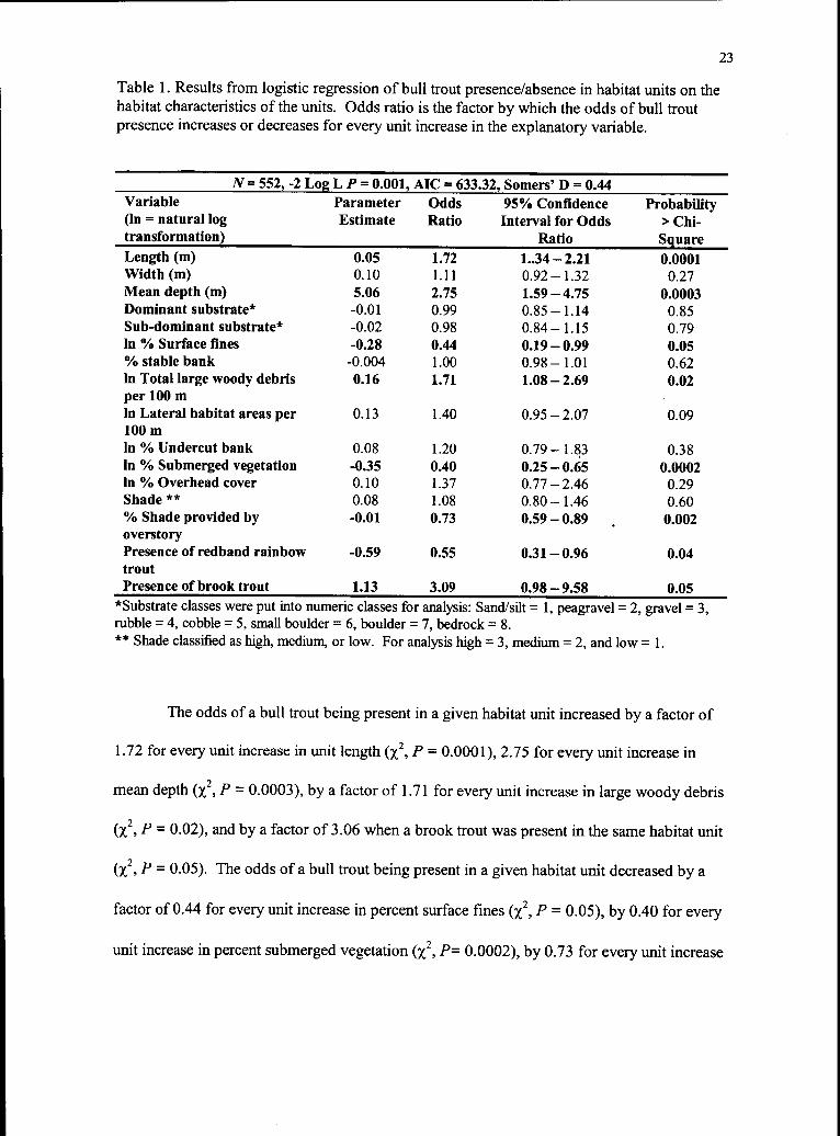
Table 1. Results from logistic regression of bull trout presence/absence in habitat units on thehabitat characteristics of the units. Odds ratio is the factor by which the odds of bull troutpresence increases or decreases for every unit increase in the explanatory variable.

N = 552, -2 Log L P = 0.001, AIC = 633.32, Somers' D = 0.44Variable(In = natural logtransformation)

ParameterEstimate

OddsRatio

95% ConfidenceInterval for Odds

Ratio

Probability> Chi-Square

Length (m) 0.05 1.72 1..34 2.21 0.0001Width (m) 0.10 1.11 0.92 1.32 0.27Mean depth (m) 5.06 2.75 1.59 4.75 0.0003Dominant substrate* -0.01 0.99 0.85 -1.14 0.85Sub-dominant substrate* -0.02 0.98 0.84 -1.15 0.79In % Surface fines -0.28 0.44 0.19 0.99 0.05% stable bank -0.004 1.00 0.98 -1.01 0.62In Total large woody debrisper 100 m

0.16 1.71 1.08 2.69 0.02

In Lateral habitat areas per 0.13 1.40 0.95 - 2.07 0.09100 mIn % Undercut bank 0.08 1.20 0.79 -1.83 0.38In % Submerged vegetation -0.35 0.40 0.25 - 0.65 0.0002In % Overhead cover 0.10 1.37 0.77-2.46 0.29Shade ** 0.08 1.08 0.80 1.46 0.60% Shade provided byoverstory

-0.01 0.73 0.59 0.89 0.002

Presence of redband rainbowtrout

-0.59 0.55 0.31 0.96 0.04

Presence of brook trout 1.13 3.09 0.98 9.58 0.05*Substrate classes were put into numeric classes for analysis: Sand/silt = 1, peagravel = 2, gravel = 3,rubble = 4, cobble = 5, small boulder = 6, boulder = 7, bedrock = 8.** Shade classified as high, medium, or low. For analysis high = 3, medium = 2, and low = 1.

The odds of a bull trout being present in a given habitat unit increased by a factor of

1.72 for every unit increase in unit length (x2, P = 0.0001), 2.75 for every unit increase in

mean depth (x2, P = 0.0003), by a factor of 1.71 for every unit increase in large woody debris

(x2, P = 0.02), and by a factor of 3.06 when a brook trout was present in the same habitat unit

(x2, P = 0.05). The odds of a bull trout being present in a given habitat unit decreased by a

factor of 0.44 for every unit increase in percent surface fines (x2, P = 0.05), by 0.40 forevery

unit increase in percent submerged vegetation (x2, P= 0.0002), by 0.73 for every unit increase

24

in the percent of shade provided by overstory (X.2, P= 0.002), and by 0.55 when a redband

rainbow trout was present in the habitat unit (x2, P = 0.04).

Analyzing all of the habitat units at once from all of the streams surveyed allowed us

to investigate within-site variation in bull trout presence/absence. Adding site catagorical

variables (i.e., patch, reach, and habitat unit type) allowed us to investigate across-site variation

in bull trout presence/absence. As evidenced by highly significant drop in deviance tests,

lower AIC, and higher Somers'D values; patch, reach, and habitat unit type categorical site

variables improved the fit of the logistic regression model over that with habitat characteristic

variables alone (Table 2).

Table 2. Comparison of models with habitat variables alone, and models with habitat variablesand patch, reach, or unit catagorical variables.

Variable Drop -in-DevianceTest for Site EffectProbability > Chi-

Square

-2 Log LikelihoodStatistic Probability

> Chi-Square

AkaikeInformation

Criterion

Somers' D

Habitat variables 0.001 633.32 0.44

Habitat variables 0.0001 0.0001 615.16 0.53

+PatchHabitat variables 0.0001 0.0001 625.21 0.61

+ReachHabitat variables 0.01 0.0001 622.19 0.48

+Unit type(Fast/Slow)

Although the categorical variables perform poorly alone in the regression model as

evidenced by high AIC and very low Somers'D scores (Table 3), patch or reach categorical

variables alone performed similarly to a model with habitat characteristic variables alone.

25

Table 3. Comparison of models with only patch, reach, or unit type catagorical variables andmodels with habitat variables alone.

Variable -2 Log Likelihood Statistic Akaike Somers' DProbability > Chi-Square Information

CriterionHabitat variables 0.001 633.32 0.44

Patch alone 0.0001 704.22 0.41

Reach Alone 0.0001 706.92 0.50Unit type (Fast/Slow) alone 0.008 760.14 0.11

Habitat variables with significant parameter estimates differ for fast and slow water

habitat unit types (Table 4). The one exception is percent of shade provided by overstory

canopy, which has a significant negative correlation to the odds of bull trout presence in fast

and slow water habitat unit types (fast water units x2, P = 0.005; odds ratio = 0.50, slow water

units x2, P = 0.006, odds ratio = 0.70). The number of pocket pools per 100 m was included

in the fast water units model because pocket pools only exist in fast water units. The parameter

estimate for pocket pools is statistically significant (x2, P = 0.03) and the odds ratio is 3.32.

The habitat unit length (x2, P = 0.0001, odds ratio = 2.23) and, total large woody debris per

100 m (x2, P = 0.01, odds ratio = 4.95) are the other two habitat variables that were significant

in the model for fast water units. In slow water units mean depth had a strong positive

relationship (x2, P = 0.01, odds ratio = 2.33) to the odds of bull trout presence in a habitat unit.

The percent surface fines (x2, P = 0.05, odds ratio = 0.40), percent submerged vegetation (x2,

P = 0.003, odds ratio = 0.40) and presence of rainbow trout (x2, P = 0.03, odds ratio = 0.47)

all had negative correlations with the odds of bull trout presence in slow water habitat units.

26

Table 4. Logistic regression models for the presence/absence of bull trout in fast water habitat

units and slow water habitat units.

FAST WATER UNITSN = 197, -2 Log L P= 0.001, AIC = 186.50, Somers' D = 0.71

Variable (In = natural logtransformation)

ParameterEstimate

OddsRatio

95% ConfidenceInterval for Odds

Ratio

Probability >Chi-Square

In Pocket poolsper 100 m***

0.37 3.32 1.13 8.16 0.03

Length (m) 0.08 2.23 1.48 3.35 0.0001

Width (in) 0.001 1.0 0.68 -1.43 0.99

Mean depth (m) -3.50 0.50 0.24 -1.01 0.49

Dominant substrate* 0.13 1.15 0.83 -1.61 0.4

Sub-dominant substrate* -0.51 0.95 0.65 -1.36 0.77

In % Surface fines 0.43 3.63 0.46 - 28.77 0.24

% Stable bank 0.009 1.01 0.98 -1.06 0.58

In Total large woodydebris per 100 m

0.48 4.95 1.55 -15.84 0.01

In Lateral habitat areasper 100 m

0.009 1.02 0.38 2.79 0.94

In % Undercut bank -0.10 0.79 0.32 -1.97 0.62

In % Submergedvegetation

-0.22 0.56 0.21 1.52 0.21

In % Overhead cover -0.04 0.88 0.23 3.42 0.87

Shade ** 0.10 1.11 0.56 2.15 0.78

% Shade provided byoverstory

-0.02 0.50 0.34 - 0.72 0.005

Presence of redbandrainbow trout

-0.71 0.49 (0.12 -1.76) 0.3

Presence of brook trout 1.66 5.31 (0.21- 68.97) 0.22

27

Table 4, Continued

SLOW WATER UNITSN = 355-2 Log L P = 0.0002, AIC = 448.60, Somers' D = 0.40

Variable (In = naturallog transformation)

ParameterEstimate

OddsRatio

95% ConfidenceInterval for Odds

Ratio

Probability>Chi-Square

Length (m) 0.01 1.11 0.48 2.52 0.66Width (m) 0.15 1.17 0.92 -1.47 0.18Mean depth (m) 4.23 2.33 1.20 4.51 0.01Dominant substrate* -0.03 0.97 0.82 -1.14 0.7Sub-dominantsubstrate*

0.009 1.01 0.84 -1.21 0.95

In % Surface fines -0.31 0.40 0.15 -1.05 0.05% Stable bank -0.01 0.99 0.97 -1.01 0.27In Total large woodydebris per 100 m

0.02 1.07 0.65 -1.75 0.69

In Lateral habitatareas per 100 m

0.13 1.41 0.87 2.27 0.16

In % Undercut bank 0.11 1.29 0.78 2.12 0.32In % Submergedvegetation

-0.35 0.40 0.21 - 0.76 0.003

In % Overhead cover 0.03 1.10 0.55 2.21 0.75Shade ** 0.01 1.02 0.72 1.45 0.92°A) Shade provided byoverstory

-0.01 0.70 0.49 -1.01 0.006

Presence of redbandrainbow trout

-0.75 0.47 0.24 0.89 0.02

Presence of brooktrout

0.92 2.53 0.68 9.74 0.16

*Substrate classes were put into numeric classes for analysis: Sand/silt = 1, peagravel = 2, gravel = 3,rubble = 4, cobble = 5, small boulder = 6, boulder = 7, bedrock = 8.** Shade classified as high, medium, or low. For analysis high = 3, medium = 2, and low = 1.***Pocket pools were not measured in slow water units.

There was a significant positive relationship between habitat unit length (x2, P =

0.0001, odds ratio = 1.62), total amount of large woody debris per 100 m (x2, P = 0.01, odds

ratio = 1.82) and the odds of juvenile bull trout presence in a habitat unit (Table 5). The

percent of submerged vegetation (x2, P = 0.005, odds ratio = 0.50), the percent of shade

provided by overstory (x2, P = 0.02, odds ratio = 0.70), and the presence of redband rainbow

trout (x2, P = 0.03, odds ratio = 0.51) were negatively correlated to the odds of bull trout

28

presence in habitat units. The presence of bull trout > 140 mm in total length (adult bull trout)

was not statistically significant (x2, P = 0.32).

Table 5. Results for logistic regression of juvenile bull trout presence/absence in habitat unitson the habitat characteristics of the units.

N = 552, - 2 Log L P = 0.0001, AIC = 614.74, Somer's D = 0.40Variable Parameter Odds 95% Probability(In = natural log transformation) Estimate Ratio Confidence > Chi-

Interval for SquareOdds Ratio

Presence of bull trout > 140 mm 0.37 1.46 0.65 2.97 0.32in total lengthLength (m) 0.04 1.62 1.34 -1.94 0.0001Width (m) 0.11 1.12 0.94 -1.36 0.23Mean depth (m) 2.39 1.61 0.78 3.33 0.1

Dominant substrate* 0.00 1 0.87 -1.16 0.98Sub-dominant substrate* -0.02 0.98 0.84 -1.17 0.84ln % Surface fines -0.17 0.60 0.25 -1.44 0.21

% Stable bank 0.00 1 0.98 -1.02 0.96In Total large woody debris per 0.18 1.82 1.14 - 2.91 0.01100 mIn Lateral habitat areas per 100 m 0.05 1.14 0.69 1.87 0.44ln % Undercut bank 0.14 1.38 0.93 2.04 0.1

In % Submerged vegetation -0.26 0.50 0.30 0.86 0.005In % Overhead cover 0.06 1.21 0.71 -2.07 0.43Shade ** -0.06 0.94 0.69 1.28 0.69% Shade provided by overstory -0.01 0.70 0.70 0.71 0.02Presence of redband rainbow -0.67 0.51 0.26 0.89 0.03troutPresence of brook trout 1.05 2.86 0.91- 9.22 0.07

*Substrate classes were put into numeric classes for analysis: Sand/silt = 1, peagravel = 2, gravel = 3,rubble = 4, cobble = 5, small boulder = 6, boulder = 7, bedrock = 8.** Shade classified as high, medium, or low. For analysis high = 3, medium = 2, and low = 1.

29

Step Two: Bull trout density of each habitat unit as the response variable

The multiple linear regression model of the natural logarithim of bull trout density (per

100 m2) in habitat units on habitat characteristic variables explained very little of the variance

in bull trout density (adjusted R2 = 0.08), however several parameter estimates were

statistically significantly larger than zero. Of the variables that were significant (P 5_ 0.05),

only mean unit depth (f3 = 1.71) and the percent surface fines (13 = -0.23) had a parameter

estimate that were substantial.

Including patch categorical variables in the model did not improve the model

significantly (lack-of-fit F-test, P = 0.13). Reach categorical variables improved the model fit

significantly (lack-of-fit F-test, P = 0.006), however the overall model fit explained little of the

variance in bull trout density (adjusted R2 = 0.23). A model that accounted for across-habitat

unit type (fast or slow water unit type) variance fit the data significantly better than one that

accounted for within-site variance alone. With habitat characteristic variables alone the

adjusted R2 = 0.09, and after adding unit type as a categorical variable the adjusted R2 = 0.45.

In other words the habitat unit type explained significantly more of the variance in bull trout

density than the specific characteristics of the habitat units alone. In fact a model with habitat

unit type catagorical variables alone performed better than a model that included quantitative

habitat characteristics. Separate multiple linear regression models for fast water units and slow

water units fit the data very poorly.

The fit of the multiple linear regression of the natural logarithm of juvenile bull trout

density (per 100 m2) in habitat units on habitat characteristic variables was poor (adjusted R2 =

0.37). However, the density of juvenile bull trout in a given habitat unit had a significant (P =

0.0001) negative correlation (3 = -0.67) with the density of adult bull trout in that same habitat

unit.

30

Reach Analysis

The saturated (i.e., contains all available variables) model of bull trout density (per 100

m2) in reaches on quantitative habitat characteristic variables fit the data poorly (ANOVA, P.

0.11, adjusted R2 = 0.34) and none of the parameter estimates were significantly larger than

zero. A reduced model was obtained by systematically removing insignificant variables (P >

0.05) until the highest adjusted R2 value was achieved (Table 6). Of the variables remaining in

the reduced model only mean summer water temperature had a large parameter estimate.

However, mean summer water temperature was only significant when a quadratic term was

included in the model. The rest of the variables that remained in the model had parameter

estimates that were very small but were significantly larger than zero (P 0.05). One

exception was the percent undercut bank, which did not have a statistically significant

parameter estimate, but dropping it from the model decreased the model fit to the data.

Models with either TEMP (TEMP= mean summer water temperature + [mean summer

water temperature ) or patch site variables alone explained approximately the same amount of

variance (Table 7; adjusted R2 = 0.39 and 0.38 respectively). A model with both TEMP and

patch variables (adjusted R2 = 0.41) explained approximately the same amount of variance as

the models with either TEMP or patch alone.

Overall model fit of multiple linear regression for juvenile bull trout density (per 100

m2) in reaches on quantitative habitat characteristic variables was moderate (adjusted R2 =

0.45) for a saturated model, however none of the parameter estimates were substantially larger

than zero. A model with a reduced set of habitat variables was obtained by systematically

removing variables with insignificant parameter estimates until the adjusted R2 value was

maximized (Table 8). All of the remaining habitat variables had parameter estimates

significantly different from zero (P S 0.05) except for density of redband rainbow trout (T-test,

P = 0.06), the density of brook trout (T-test, P = 0.48) and the percent of undercut bank (T-

31

test, P = 0.13). Despite the statistical significance of the parameter estimates most of them

were very small (Table 8). Mean water temperature and density of adult bull trout were two

exceptions. Mean summer water temperature was not significant without a quadratic term

included in the model. Juvenile bull trout density in reaches was positively correlated with

adult bull trout densities (parameter estimate = 0.53, T-test, P = 0.05).

Table 6. Results of the best fit multiple linear regression model of (1n) bull trout density on thehabitat characteristic of the reaches.

N= 32, R2 = 0.67, Adjusted R2 = 0.59, ANOVA P= 0.0001Variable (In = natural log Parameter 95% Confidence Probability >transformation) Estimate Interval for T Statistic

ParameterEstimate

Mean summer water temperature (°C) 5.24 2.89 - 7.59 0.0001(Mean summer water temperature)2 (°C) -0.35 -0.50 - (-0.20) 0.004Mean dominant substrate -0.15 -0.32 - 0.01 0.07% Surface fines -0.02 -0.03- (-0.01) 0.005% Undercut bank 0.02 -0.01 0.05 0.23In % Submerged vegetation -0.02 -0.03 - (-0.01) 0.002

Table 7. Comparison of fit for models with mean summer water temperature alone, patchalone, and mean summer water temperature and patch together.

Explanatory R2 and Adjusted R2 ANOVA F-Test Lack-of-Fit F-TestVariables

TEMP* R2 = 0.43, Adj. R2 = 0.39 P= 0.0002PATCH R2 = 0.53, Adj. R2 = 0.38 P= 0.008TEMP + PATCH R2 = 0.59, Adj. R2 = 0.41 P = 0.01 PATCH P= 0.007

TEMP P > 0.1*TEMP = mean summer water temperature + (mean summer water temperature)2

32

Table 8. Results of the best fit multiple linear regression model of (1n) juvenile bull trout density

on the habitat characteristic of the reaches.

N = 32, R2 = 0.76, adjusted R2 = 0.62, ANOVA P = 0.0005Variable (ln = natural logtransformation)

ParameterEstimate

95% ConfidenceInterval for

Parameter Estimate

Probability >T Statistic

Density of bull trout with > 140 mm totallength

0.53 0.01 1.05 0.05

Mean summer water temperature (°C) 3.78 0.67- 6.90 0.02

(Mean summer water temperature)2 (°C) -0.24 -0.45 (-0.04) 0.02

% Surface fines -0.01 -0.03 - (-0.002) 0.03

Total large woody debris per 100 m 0.02 0.002 - 0.05 0.04

ln Lateral habitat areas per 100 m -0.18 -0.37 - (-0.003) 0.05

% Undercut bank 0.03 -0.01 0.07 0.13

% Overhead cover -0.02 -0.03 (-0.01) 0.004

In % Submerged vegetation -0.02 -0.03 - (-0.01) 0.007

% Shade provided by overstory -0.01 -0.01 - 0.001 0.07

Density of redband rainbow troutper 100 m2

-0.26 -0.53 0.01 0.06

Density of brook trout per 100 m2 -0.28 -1.10 0.54 0.48

Patch Analysis

Various combinations of quantitative habitat variables were added and removed from

a multiple linear regression model ofbull trout density in patches on habitat characteristics

until a final model was constructed which explained the most variance in the data. The final

model contained stream gradient, and TEMP (TEMP= mean summer water temperature +

[mean summer water temperature ) as explanatory variables and fit the data well (Table 9;

adjusted R2 = 0.74 ). After accounting for gradient there is a strong quadratic relationship

between bull trout density and mean summer water temperature. Table 10 gives the results

from multiple linear regression of juvenile bull trout density on gradient and mean summer

water temperature. Again various combinations of quantitative habitat variables were added

and removed from the model until a final model was constructed that explained the most

variance in the data. The final model included the same explanatory variables as the model

with juvenile and adult bull trout as the response variable, however the model with juvenile

33

bull trout density as the response variable explained more of the variance (adjusted R2 = 0.87).

After accounting for gradient there was a strong quadratic relationship between juvenile bull

trout density and mean summer water temperature.

Table 9. Results of multiple linear regression of bull trout density in patches on the habitatcharacteristics of the patches.

N = 9, R2 = 0.84, adjusted R2 = 0.74, ANOVA P = 0.02Variable (ln = natural log Parameter 95% Confidence Interval for Probability > Ttransformation) Estimate Parameter Estimate StatisticGradient 0.17 0.01 0.33 0.04Mean summer watertemperature (°C)

8.87 1.77 15.97 0.02

(Mean summer watertemperature)2 (°C)

-0.6 -1.06 (-0.15) 0.02

Table 10. Results of multiple linear regression of juvenile bull trout density in patches on thehabitat characteristics of the patches.

N = 9, R2 = 0.92, adjusted R2 = 0.87, ANOVA P = 0.004Variable On = natural log Parameter 95% Confidence Interval Probability > Ttransformation) Estimate for Parameter Estimate StatisticGradient 0.11 0.02 0.19 0.02Mean summer watertemperature (°C)

9.64 5.79 13.50 0.001

(Mean summer watertemperature)2 (°C)

-0.63 -0.88 (-0.39) 0.001

34

DISCUSSION

Fish Counts: Day vs. Night and Size Distribution

Overall the day counts of bull trout were proportional to night counts of bull trout,

which indicates that day counts were precise enough for comparisons of relative abundance.

The day snorkel counts were lower than the number of bull trout counted at night (Figure 3).

The tendency for bull trout to conceal during the day and emerge from cover at night is highly

variable from stream to stream and from age class to age class. Several authors reported higher

counts of bull trout during night snorkel counts than during day snorkel counts (Jakober 1995;

Goetz 1997; Sexauer and James 1997). Others could not find statistically significant

differences in day versus night snorkel counts of bull trout (Thurow and Schill 1996; Adams

1994). As water temperature warms above about 7°C, daytime bull trout counts tend to

increase (Bonneau et al. 1995; Jakober 1995). Goetz (1997c) found that diel patterns in bull

trout concealment vary with age class. Thurow and Schill (1996) and Adams (1994)

snorkeled at temperatures above 9 and 8°C respectively and could not find significant

differences in night and day counts. Baxter and McPhail (1997) documented a diel habitat

shift in juvenile bull trout held in a laboratory stream where temperatures were below 9°C.

In addition to detecting fewer bull trout than night surveys, the daytime surveys were

biased towards bull trout that were approximately 110 mm in total length and larger. The

downward sloping left leg of the bell-shaped frequency histogram displayed in Figure 4

indicates that bull trout less than approximately 110 mm in total length remain concealed from

divers. The tendency for small bull trout, especially young of the year, to go undetected by

surveyors is not unique to our streams or to day snorkeling methods. In a survey of recent

literature that included length-frequency histograms I found similar bell-shaped patterns even

when the sampling method was night snorkeling or multiple pass electrofishing (Hemmingsen

35

et al. 1996; Thurow and Schill 1996; Hunt et al. 1997; Sexauer and James 1997; Stelfox

1997). The frequency of the bell-shaped pattern in bull trout length-frequency histograms

highlights the tendency of juveniles to often remain in contact with the substrate or concealed

within some form of cover (Pratt 1984; Adams 1994; Bonneau 1994; Jakober 1995; Baxter

and McPhail 1997; Sexauer and James 1997; Thurow 1997). We can conclude that there are

site specific differences in temporal, age class, and temperature related patterns in bull trout

concealment behavior. These site-specific logistic challenges should be recognized when

designing sampling methodologies or analyzing demographic data.

Patterns at Multiple Spatial Scales

The significance of habitat characteristic and site categorical variables in logistic and

multiple linear regression models indicate that the habitat characteristics of individual habitat

units as well as factors evaluated at larger spatial scales are related to bull trout

presence/absence and density in habitat units.

The significance of habitat variables differed between fast and slow water habitat

units, suggesting that there are complex relationships between habitat characteristics and bull

trout abundance. The characteristics of habitat units, such as cover, velocity breaks, food

availability, and other features necessary for survival of individuals, can directly influence fish

presence and density. The statistically significant positive correlation between habitat unit

length and bull trout presence in fast water habitat units is logical. The longer the habitat unit

(some fast water habitat units were 100 m long) the higher the likelihood a bull trout will be

present because a greater amount of area has been searched. The mean depth of slow water

habitat units had a strong positive correlation to bull trout presence in habitat units. Several

authors have documented the bull trout's affinity for low velocity habitat (Pratt 1984; Adams

1994; Bonneau 1994; Jakober 1995; Rich 1996; Sexauer and James 1997). Pools and low

36

velocity runs were often the deepest habitat units in our study area. Therefore, the strong

positive correlation between unit depth and bull trout presence and density may be related to

their preference for pools and other low velocity units. When fast and slow water habitat units

were analyzed separately, mean depth was only significant in slow water units indicating the

importance of pool depth. One reason bull trout may prefer deep habitat units is that they may

provide cover from terrestrial predators (Lonzarich and Quinn 1995).

The positive correlation between bull trout presence and total large woody debris is

consistent with other reports of strong associations between bull trout and large woody debris

(Goetz 1991; Jakober 1995; Dambacher and Jones 1997). When slow and fast water habitat

units were analyzed separately, LWD was only significant in fast water units. Large woody

debris in fast water units may provide velocity breaks that affords holding areas for bull trout

in otherwise high velocity areas.

Pocket pools are found only in fast water habitat units. The number of pocket pools

had a strong positive correlation to the presence of bull trout in habitat units. In fact 32 % of

the bull trout in fast water habitat units were observed holding in pocket pools, while only 17

% of redband rainbow trout observed in fast water units were in pocket pools. Saffel and

Scarnecchia (1995) also found a positive correlation between juvenile adfluvial bull trout

density and the number of pocket pools.

The percent surface fines in slow water habitat units had a strong negative correlation

to bull trout presence in slow water habitat units. There was not a relationship between percent

surface fines and bull trout presence or density in fast water units. Bjornn and others (1977)

found that higher levels of sediment resulted in reduced densities of fish in laboratory and

natural stream pools, but could not find significant correlations in riffles. Fine sediment can

fill interstitial spaces between bed material that would otherwise be used by bull trout for cover

from predators (Bjornn et al. 1977; McPhail and Murray 1979; Baxter and McPhail 1997;

37

Thurow 1997). Pratt (1984) reported that juvenile bull trout defended territories over the

streambed. When interstitial areas in the streambed are filled with sediment, bull trout may be

forced into positions within the water column where they must defend territories or leave the

area. One of the most common themes in the literature on migratory and resident bull trout

involves the importance of substrate as cover (Pratt 1984; Adams 1994; Bonneau 1994;

Jakober 1995; Baxter and McPhail 1997; Sexauer and James 1997; Thurow 1997).

The significance of substrate related habitat characteristics in this study support the

growing evidence found in the literature. In this study divers repeatedly commented on the

tendency for bull trout (especially juveniles) to remain motionless in direct contact with the

substrate when disturbed. This behavior is similar to sculpin behavior and is in contrast to

redband rainbow trout and brook trout that tend to flee rather than lie motionless. I noticed

that bull trout were easier to detect when they were lying motionless in smaller substrates, such

as sand and silt. Road construction, logging, livestock grazing, mining and other management

activities can contribute directly to increased sediment levels and consequent embeddedness in

stream channels (Bjornn et al. 1977). The soils of the Idaho Batholith are particularly

susceptible to erosion (Wendt et. al 1973; Arnold 1975), which may increase the risk to bull

trout because of their potential sensitivity to alterations of substrate size class structure.

There are two likely reasons for the negative correlation between bull trout presence

and the percent of submerged vegetation. Fish may be avoiding detection by the divers by

hiding in the thick vegetation. Another possibility is that the high percent of submerged

vegetation is indirectly associated with warmer water temperatures, which has a parabolic

correlation to bull trout densities at larger spatial scales.

The percent of shade provided by overstory does not indicate the total amount of

stream shade, instead it gives an estimate of what percent of the stream shade is provided by

large coniferous trees as opposed to small alder, willow, and herbaceous plants (understory).

38

The negative correlation between juvenile and adult bull trout presence in habitat units and the

percent of shade provided by overstory may be related to a lack ofunderstory rather than the

amount of overstory. Alder and willow often hang over the stream providing shade as well as

cover from terrestrial predators.

The negative correlation between redband rainbow trout presence and bull trout

presence may be related to competitive displacement or differences in temperature preferences

between the two species. Divers observed very few aggressive interactions between the two

species, however the two species are known to segregate spatially across a temperature gradient

(Ziller 1992; Adams 1994; Lowman Ranger District unpublished data). Brook trout are

considered a threat to bull trout population persistence through hybridization and potential

competitive interactions (Rieman and McIntyre 1993). The positive correlation between the

brook trout presence and the presence of bull trout in a habitat unit may be due in part to

similar preferences for habitat types. Also there were very few units with brook trout that did

not have bull trout because of the larger overlap in the temperature preferences of the two

congeners.

Bull trout had higher densities in slow water habitat than in fast water units. In fact

habitat type (fast or slow) had a stronger correlation to bull trout density than the habitat

characteristics of the habitat units such as the amount of large woody debris, mean depth,

percent surface fines, and so on. The significance of the habitat unit type categorical variable

indicates that factors associated with fast and slow units that we did not measure are

influencing bull trout presence/absence and density in addition to the variables we measured.

These factors may include water velocity, which was not directly measured in each habitat unit.

It is also possible that snorkeling counts are biased to some degree in fast water units because

they are often shallow and therefore difficult to snorkel effectively.

39

Reach categorical variables were highly significant at the habitat unit scale indicating

that factors at the reach scale were influencing bull trout presence and density in habitat units.

Of the habitat variables included in reach scale multiple linear regression models, mean

summer water temperature and a quadratic term for mean summer water temperature were the

only coefficients with large values that were statistically significant. Thus, mean summer water

temperature is likely one of the key factors at the reach scale that is influencing bull trout

densities. Decreasing stream sizes may confound the parabolic relationship between bull trout

density and mean summer water temperature. In other words, the decrease in bull trout

densities in reaches with mean summer water temperatures below about 7°C may in part result

because the reaches with the coldest temperatures are often near the source of the stream where

the small channel size limits the suitability of the habitat. Saffel and Scarnecchia (1995) found

a decreasing trend in the density of juvenile adfluvial bull trout in 100 m reaches with the

coldest maximum summer stream temperatures. I failed to find any literature documenting bull

trout physiological performance at extremely cold temperatures. Patch categorical variables

were also very significant. In fact patch categorical variables explained the variation in bull

trout density equally as well as summer mean water temperature.

The high significance and large proportion of variance explained by the patch

categorical variables in the reach scale model suggests factors at the patch scale have a strong

relationship to the density of bull trout in reaches. In other words, bull trout density in reaches

within patches are not entirely independent. Mean summer water temperature is a likely factor

influencing bull trout density at the patch scale. Other potential unmeasured factors thatmay

be contributing to the remaining variation in bull trout density (i.e., not explained by

temperature) include differences in stream productivity, random bull trout population

fluctuations, and sampling error. Gradient had a positive correlation to bull trout density in

patches, however the relationship was a weak one. After accounting for stream temperature,

40

bull trout may be less abundant in lower gradient streams because of lack of large substrate and

other forms of cover often associated with complex moderate to high gradient streams. Rich

(1996) found a strong negative correlation between bull trout presence and gradient, however

his sample was not confined to habitat that was known to be occupied by bull trout. My results

apply only to habitat characteristics within patches occupied by bull trout

The highest densities of bull trout in this study were in reaches with mean summer

stream temperatures between 7 and 8.5°C (Figure 5). It is clear from laboratory and field

evidence that cold temperatures are crucial for juvenile bull trout growth and survival (McPhail

and Murray 1979; Saffel and Scarnecchia 1995; Goetz 1997a). We also found temperature to

be highly significant in patch scale models with juvenile bull trout as the response variable.

5.00

4.50

_4.00-i-8._ 3.50

3.00

zcn

0LA, 2.50 1

5O 2.00

..., 1.50mco a

1.00 -

0.50

0.00

6.00 6.50 7.00 7.50 8.00 8.50 9.00 9.50

MEAN SUMMER STREAM TEMPERATURE (°c)

Figure 5. Scatter plot of bull trout density in reaches vs. the mean summer stream temperature.

There is also some evidence that the species segregation that is commonly found in streams

with bull trout and other salmonids is in part the result of a shift in competitive dominance at

41

various temperatures. Adams (1994) found juvenile and adult bull trout in a meadow stream

that reached 20.5°C at least three days in a row. I observed bull trout feeding and cruising in a

stream that was 23.5°C and likely over 24°C during the warmest part of the day. In both

circumstances bull trout were the only salmonid species observed. Bull trout distribution may

be confined to colder streams when other salmonid species are present because their ability to

compete for resources improves. Further research is needed on the physiological performance

of bull trout over a wide temperature gradient and in the presence of various other salrnonid

competitors. Knowing the maximum and minimum temperature tolerances of all age classes

of bull trout may be a helpful tool in predicting bull trout occurrence.

Juvenile bull trout presence in habitat units was not significantly correlated in any way

with the presence of adult bull trout, however the density of juvenile bull trout in a habitat unit

had a strong negative correlation with the density of adult bull trout in the unit. Bull trout are

highly piscivorous and often cannibalistic (Goetz 1989; Goetz 1997b; author's personal

observation). When densities of adult bull trout are high in a habitat unit, juvenile bull trout

may conceal themselves or leave the unit. At the reach scale, the density of juvenile bull trout

was positively correlated to adult bull trout density. These results contradict the negative

correlation found between juvenile bull trout density in habitat units. These results underscore

the importance of scale in fish habitat relationships. Interactions between bull trout within a

stream may directly effect their distribution within specific habitat units, but have little effect

on the overall density of the population at larger spatial scales such as reaches.

Large-scale factors may constrain the effectiveness of small-scale habitat projects such

as adding LWD to streams. For example the mean temperature of a patch may be the limiting

factor that constrains the density of bull trout in individual reaches and habitat units, but

temperature is partly controlled by large-scale watershed attributes, such as aspect and

42

elevation, which are beyond the control of managers. Adding LWD to a stream that is too

warm for bull trout will not likely increase the abundance of bull trout.

One important implication of large scale controlling factors in fish populations is that

the controlling factors act on the population as a whole. For example, as long as fish have

freedom to move, distribution and density in habitat units and reaches (or whatever spatial unit

one chooses) within a stream are not independent of one another (Gowan et al. 1993). In our

study, temperature may be a large-scale factor that is contributing to fish distribution and

density within habitat units and reaches throughout patches. Recent work on bull trout

populations has emphasized the potential role of metapopulation dynamics in population

persistence (Rich 1996; Dunham and Rieman 1999). To the degree that metapopulation

dynamics are operating, bull trout distribution and density may be linked across patches within

watersheds or even entire basins. Stream temperature within a given patch of bull trout habitat

has the potential to affect the population dynamics in adjacent patches.

Dunham and Rieman (1999) and Rich (1996) documented strong relationships

between the area of suitable habitat and the presence of bull trout. Both papers stated the

importance of conservation of core bull trout areas. When designating core areas for

protection, large-scale factors that constrain bull trout populations should be considered. It

would be wise to consider features of the landscape beyond catchment or basin size that will

influence bull trout population size. For example, does the patch have the characteristics

necessary to produce and maintain water temperatures that will contribute to strong bull trout

populations?

Within certain constraints bull trout can inhabit a diversity of habitat types. Indeed

bull trout could not have obtained their current distribution without having strong tendencies to

colonize new habitat and recolonize previously occupied habitat. With these traits in mind

managers should remain optimistic about restoring and conserving bull trout populations.

43

This study was observational in nature. Therefore we cannot infer that the linear

correlations between resident bull trout density and the explanatory variables we measured and

found to be statistically significant are direct cause and effect relationships. Controlled

experiments are needed to test for causal relationships between the habitat characteristics we

found to be significant, such as temperature, and bull trout distribution and density.

44

BIBLIOGRAPHY

Adams, S. B. 1994. Bull trout distribution and habitat use in the Weiser River drainage,Idaho. Master's Thesis, University of Idaho, Moscow.

Arnold, J. F. 1975. Appendix B of the Idaho Batholith source book: descriptions ofsections and subsections of that portion of the northern rocky mountain physiographicprovince containing the Idaho Batholith. U.S.D.A., Forest Service, IntermountainRegion.

Baxter, J. S., and J. D. McPhail. 1997. Diel microhabitat preferences of juvenile bull trout inan artificial stream channel. North American Journal of Fisheries Management.17:975-980.

Beschta, R. L., and W. S. Platts. 1986. Morphological features of small streams: significanceand function. Water Resources Bulletin. 22(3): 369-380.

Bjornn, T. C., M. A. Brusven, M. P. Molnau, J. H. Milligan, R Klamt, E Chacho, and C.Schaye. 1977. Transport of granitic sediment in streams and its effects on insects andfish. Research Technical Completion Report, Project B-036-IDA. Contribution No.59, Forest, wildlife and Range Experiment Station. Contribution No. 7762,Agricultural Experiment Station. University of Idaho, Moscow.

Bonneau J. L., R. F. Thurow, and D. L. Scarnecchia. 1995. Capture, marking, and enumerationof juvenile bull trout and cutthroat trout in small, low-conductivity streams. NorthAmerican Journal of Fisheries Management. 15:563-568.

Bonneau, J. L. 1994. Seasonal habitat use and changes in distribution of juvenile bull trout andcutthroat trout in small, high gradient streams. Master's Thesis, University of Idaho,Moscow.

Cavender, T. M. 1978. Taxonomy and distribution of the bull trout (Salvelinus confluentus)from the American Northwest. California Fish and Game. 64(3):139-174.

Dambacher, J. M., and K. Jones. 1997. Stream habitat of juvenile bull trout populations inOregon and benchmarks for habitat quality. Pages 353-360 in Mackay, W. C., M. K.Brewin, and M. Monita, eds. Friends of the bull trout conference proceedings. BullTrout Task Force (Alberta), c/o Trout Unlimited Canada, Calgary.

Dunham, J. B., and G. L. Vinyard. 1997. Incorporating stream-level variability into analyses offish habitat relationships: some cautionary examples. Transactions of the AmericanFisheries Society. 126:323-329

Dunham, J. B., and B. E. Rieman. 1999. Metapopulation structure of bull trout: influences ofhabitat size, isolation, and human disturbance. Ecological Applications. 9:642-655.

Frissell, C. A., W. J. Liss, and C. E. Warren, and M. D. Hurley. 1986. A hierarchicalframework for stream habitat classification: viewing streams in a watershed context.Environmental Management. 10:199-214.

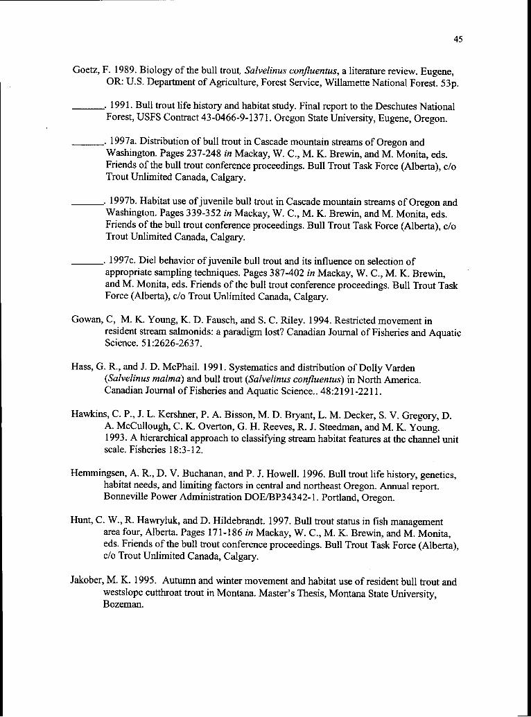
45

Goetz, F. 1989. Biology of the bull trout, Salvelinus confluentus, a literature review. Eugene,OR: U.S. Department of Agriculture, Forest Service, Willamette National Forest. 53p.

. 1991. Bull trout life history and habitat study. Final report to the Deschutes NationalForest, USFS Contract 43-0466-9-1371. Oregon State University, Eugene, Oregon.

1997a. Distribution of bull trout in Cascade mountain streams of Oregon andWashington. Pages 237-248 in Mackay, W. C., M. K. Brewin, and M. Monita, eds.Friends of the bull trout conference proceedings. Bull Trout Task Force (Alberta), doTrout Unlimited Canada, Calgary.

1997b. Habitat use of juvenile bull trout in Cascade mountain streams of Oregon andWashington. Pages 339-352 in Mackay, W. C., M. K. Brewin, and M. Monita, eds.Friends of the bull trout conference proceedings. Bull Trout Task Force (Alberta), doTrout Unlimited Canada, Calgary.

. 1997c. Diel behavior of juvenile bull trout and its influence on selection ofappropriate sampling techniques. Pages 387-402 in Mackay, W. C., M. K. Brewin,and M. Monita, eds. Friends of the bull trout conference proceedings. Bull Trout TaskForce (Alberta), do Trout Unlimited Canada, Calgary.

Gowan, C, M. K. Young, K. D. Fausch, and S. C. Riley. 1994. Restricted movement inresident stream salmonids: a paradigm lost? Canadian Journal of Fisheries and AquaticScience. 51:2626-2637.

Hass, G. R., and J. D. McPhail. 1991. Systematics and distribution of Dolly Varden(Salvelinus malma) and bull trout (Salvelinus confluentus) in North America.Canadian Journal of Fisheries and Aquatic Science.. 48:2191-2211.

Hawkins, C. P., J. L. Kershner, P. A. Bisson, M. D. Bryant, L. M. Decker, S. V. Gregory, D.A. McCullough, C. K. Overton, G. H. Reeves, R. J. Steedman, and M. K. Young.1993. A hierarchical approach to classifying stream habitat features at the channel unitscale. Fisheries 18:3-12.

Hemmingsen, A. R., D. V. Buchanan, and P. J. Howell. 1996. Bull trout life history, genetics,habitat needs, and limiting factors in central and northeast Oregon. Annual report.Bonneville Power Administration DOE/BP34342-1. Portland, Oregon.

Hunt, C. W., R. Hawryluk, and D. Hildebrandt. 1997. Bull trout status in fish managementarea four, Alberta. Pages 171-186 in Mackay, W. C., M. K. Brewin, and M. Monita,eds. Friends of the bull trout conference proceedings. Bull Trout Task Force (Alberta),c/o Trout Unlimited Canada, Calgary.

Jakober, M. K. 1995. Autumn and winter movement and habitat use of resident bull trout andwestslope cutthroat trout in Montana. Master's Thesis, Montana State University,Bozeman.

46

Lonzarich, D. G., and T. P. Quinn. 1995. Experimental evidence for the effect of depth andstructure on the distribution, growth, and survival of stream fishes. Canadian Journalof Zoology. 73:2223-2230.

McPhail, J. D., and C. Murray. 1979. The early life history and ecology of Dolly Varden(Salvelinus malma) in the upper Arrow Lakes. Report to the British Columbia Hydroand Power Authority and Kootenay Department of Fish and Wildlife, Vancouver.

Moore, K. M. S., and S. V. Gregory. 1988. Response of young-of-the-year cutthroat trout tomanipulation of habitat structure in a small stream. Transactions of the AmericanFisheries Society. 117:162-170.

Northcote, T. G. 1992. Migration and residency in stream salmonids: some ecologicalconsiderations and evolutionary consequences. Nordic Journal of Freshwater Research67:5-17.

Overton, K. C., J. D. McIntyre, R. Armstrong, S. L. Whitwell, and K. A. Duncan. 1995.User's guide to fish habitat: Descriptions that represent natural conditions in theSalmon River Basin, Idaho. USDA Forest Service, Intermountain Research Station,General Technical Report INT -GTR -322, Ogden, Utah.

Overton, K. C., S. P. Wollrab, B. C. Roberts, M. A. Radko. 1997. R1/R4 [NorthernRegion/Intermountain Region] fish and fish habitat standard inventory procedureshandbook. Gen. Tech. Rep. 1NT- GTR-346. Ogden, UT: U.S. Department ofAgriculture, Forest Service, Intermountain Research Station. '73p.

Pratt, K .L. 1984. Habitat use and species interactions of juvenile cutthroat (Salmo clarkilewisi) and bull trout (Salvelinus confluentus) in the Upper Flathead River basin.Master's Thesis, University of Idaho, Moscow.

Ramsey, F. L., and D. W. Schafer. 1997. The statistical sleuth: a course in methods of dataanalysis. Wadsworth Publishing Company, Belmont, CA.

Rich, C. F. Jr. 1996. Influence of abiotic and biotic factors on occurrence of resident bull troutin fragmented habitats, Western Montana. Master's Thesis, Montana State University,Bozeman.

Rieman, B. E. and J. D. McIntyre. 1993. Demographic and habitat requirements forconservation of bull trout. USDA Forest Service, Intermountain Research Station,General Technical Report INT-302, Ogden, Utah.

. 1995. Occurrence of bull trout in naturally fragmented habitat patches of varied size.Transactions of the American Fisheries Society 124:285-296.

Saffel, P. D., and D. L. Scarnecchia. 1995. Habitat use by juvenile bull trout in Belt-Seriesgeology watersheds of northern Idaho. Northwest Science. 69(4): 304-317

SAS logistic regression examples: using the SAS system. Version 6, First edition. SAS InstituteInc., Cary, NC.

47

Schlosser, I. J. 1995. Critical landscape attributes that influence fish population dynamics inheadwater streams. Hydrobologia. 303:71-81

. 1991. Stream fish ecology: a landscape perspective. BioScience 41:704-712

Sexauer, H. M. and P. W. James. 1997. Spawning behavior, spawning habitat and alternativemating strategies in an adfluvial population of bull trout. Pages 325-329 in Mackay,W. C., M. K. Brewin, and M. Monita, eds. Friends of the bull trout conferenceproceedings. Bull Trout Task Force (Alberta), c/o Trout Unlimited Canada, Calgary.

Stelfox, J. D. 1997. Seasonal movement, growth, survival and population status of theadfluvial bull trout population in lower Kananaskis Lake, Alberta. Pages 309-316 inMackay, W. C., M. K. Brewin, and M. Monita, eds. Friends of the bull troutconference proceedings. Bull Trout Task Force (Alberta), c/o Trout Unlimited Canada,Calgary.

Thurow, R. F. 1997. Habitat utilization and diel behavior of juvenile bull trout (Salvelinusconfluentus) at the onset of winter. Ecology of Freshwater Fish. 6:1-7.

. 1994. Underwater methods for study of salmonids in the Intermountain West. Gen.Tech. Rep. INT -GTR -307. Ogden, UT: U.S. Department of Agriculture, ForestService, Intermountain Station. 23p.

Thurow, R. F., and D. J. Schill. 1996. Comparisons of day snorkeling, night snorkeling, andelectrofishing to estimate bull trout abundance and size structure in a second-orderIdaho stream. North American Journal of Fisheries Management. 16:314-323.

Watson, G., and T. Hillman. 1997. Factors affecting the distribution and abundance of bulltrout: an investigation at hierarchical scales. North American Journal of FisheriesManagement. 17:237-252.

Wendt, G. E., R. A. Thompson, and K. N. Larson. 1975. Land systems inventory: BoiseNational Forest Idaho. U.S.D.A., Forest Service, Intermountain Region.

Western Regional Climate Center web site. 1998. http://www.wrcc.dri.edu/index.html.

Ziller, J. S. 1992. Distribution and relative abundance of bull trout in the Sprague Riversubbasin, Oregon. In Howell, P.J., and D.V. Buchanan, eds. Proceedings of theGearhart Mountain bull trout workshop; 1992 August; Gearhart Mountain, OR.Corvallis, OR: Oregon Chapter of the American Fisheries Society: 18-29.

48

APPENDIX

49

Table A.1. Results for multiple linear regression of (ln) bull trout density per 100 m2 in habitatunits on the habitat characteristics of the habitat units.

N= 165, R2 = 0.17, Adjusted R2 = 0.08, ANOVA P = 0.0132Variable Parameter 95% Confidence Probability > T(ln = natural log Estimate Interval for Parameter Statistictransformation) EstimateMean depth (m) 1.71 0.34 3.09 0.02Dominant substrate* -0.08 -0.16 0.00 0.05Sub-dominant substrate* -0.006 -0.09 0.08 0.89In % Surface fines -0.23 -0.38 (-0.08) 0.003Vo Stable bank -0.01 -0.02 0.00 0.03In Total large woodydebris per 100 m

0.09 0.01 0.17 0.03

In Lateral habitat areasper 100 m

-0.01 -0.09 0.07 0.77

In % Undercut bank 0.01 -0.08 0.11 0.81In % Submergedvegetation

0.06 -0.11 0.12 0.89

In % Overhead cover 0.07 -0.03 0.17 0.18Shade** 0.1 -0.04 0.25 0.16% Shade provided byoverstory

0 -0.003 0.003 0.99

Presence of redbandrainbow trout

-0.11 -0.44 0.21 0.5

Presence of brook trout -0.14 -0.72 0.43 0.63*Substrate classes were put into numeric classes for analysis: Sand/silt = 1, peagravel = 2, gravel = 3,rubble = 4, cobble = 5, small boulder = 6, boulder = 7, bedrock = 8.** Shade classified as high, medium, or low. For analysis high = 3, medium = 2, and low = 1.

50

Table A.2. Separate multiple linear regression models for the (ln) density of bull trout in fastwater habitat units and slow water habitat units.

Variable (In = naturallog transformation)

FAST WATER UNITSANOVA F-Test P= 0.16,R2 = 0.44, Adjusted R2= 0.15,N= 45

Parameter ProbabilityEstimate > T Statistic

(95 % CI)

SLOW WATER UNITSANOVA F-Test P= 0.007,R2 = 0.24, Adjusted R2 = 0 .14,N= 120

Parameter ProbabilityEstimate > T Statistic

(95 % C.I.)In Pocket pools per 0.03 (-0.15 0.21) 0.73100 mMean depth (m) -3.9 (-9.5 1.68) 0.16 -0.55 (-1.67 0.57) 0.33Dominant substrate* -0.19 0.03 0.02 (-0.05 0.08) 0.61

(-0.36 (-0.02))Sub-dominant -0.003 0.97 0.04 (-0.04 0.11) 0.31substrate* (-0.19 0.18)ln % Surface fines -0.41 (-0.86 0.04) 0.07 -0.1 (-0.22 0.01) 0.08% Stable bank 0.005 (-0.02 0.03) 0.61 -0.01 0.007

(-0.02 (-0.003)ln Total large woodydebris per 100 mln Lateral habitatareas per 100 m

0.26 (0.02 0.49)

-0.11 (-0.29 0.06)

0.03

0.19

0.05 (-0.01 0.11)

0.02 (-0.04 0.09)

0.08

0.44

In % Undercut bank -0.18 (-0.37 0.01) 0.07 0.03 (-0.05 0.11) 0.41In % Submergedvegetation

0.08 (-0.26 0.42) 0.64 0.04 (-0.05 0.13) 0.33

In % Overhead cover -0.06 (-0.34 0.21) 0.64 0.1 (0.02 0.18) 0.01Shade** 0.08 (-0.22 0.37) 0.59 0.06 (-0.06 0.18) 0.31% Shade provided by -0.004 0.22 0.001 0.26overstory (-0.004 - 0.003) (-0.001 0.005)Presence of redbandrainbow trout

-0.26 (-0.89 0.35) 0.39 -0.05 (-0.32 0.22) 0.71

Presence of brooktrout

-0.34 (-2.17 1.48) 0.7 -0.07 (-0.51 0.36) 0.73

*Substrate classes were put into numeric classes for analysis: Sand/silt = 1, peagravel = 2, gravel = 3,rubble = 4, cobble = 5, small boulder = 6, boulder = 7, bedrock = 8.** Shade classified as high, medium, or low. For analysis high = 3, medium = 2, and low = 1.

51

Table A.3. Results for multiple linear regression of (1n) juvenile bull trout density in habitatunits on the habitat characteristics of the units.

N =165, R2 = 0.43, Adjusted R2 = 0.37, ANOVA P=.0001Variable(ln = natural log transformation)

ParameterEstimate

95% ConfidenceInterval forParameterEstimate

Probability >T Statistic

Density of bull trout > 140 mm intotal length per 100 m2

-0.67 -0.83 (-0.52) 0.0001

Mean depth (m) 1.6 -11 -3.30 0.07Dominant substrate* -0.05 -0.15 0.04 0.26Sub-dominant substrate* -0.02 -0.13 0.08 0.66In % Surface fines -0.18 -0.36 0.003 0.05% Stable bank -0.01 -0.03 0.001 0.03ln Total large woody debris per 100m

0.08 0.01- 0.17 0.09

In Lateral habitat areas per 100 m -0.01 -0.11 0.08 0.77In % Undercut bank 0.07 -0.04 0.18 0.21ln % Submerged vegetation -0.01 -0.15 0.12 0.83In % Overhead cover 0.06 -0.05 0.18 0.28Shade** 0.05 -0.12 -0.22 0.54% Shade provided by overstory 0.002 -0.002 0.01 0.31Presence of redband rainbow trout -0.15 -0.53 0.24 0.45Presence of brook trout -0.21 -0.88 0.45 0.53

*Substrate classes were put into numeric classes for analysis: Sand/silt = 1, peagravel = 2, gravel = 3,rubble = 4, cobble = 5, small boulder = 6, boulder = 7, bedrock = 8.** Shade classified as high, medium, or low. For analysis high = 3, medium = 2, and low = 1.

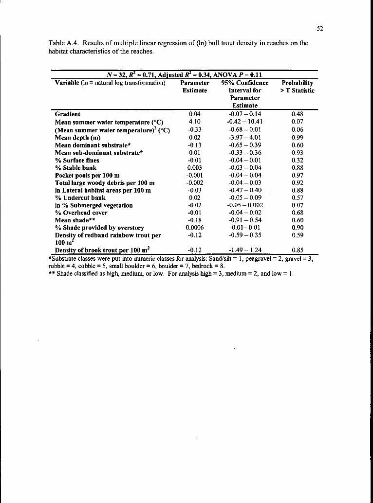
52

Table A.4. Results of multiple linear regression of (1n) bull trout density in reaches on thehabitat characteristics of the reaches.

N = 32, R2 = 0.71, Adjusted R2 = 0.34, ANOVA P = 0.11Variable (In = natural log transformation) Parameter

Estimate95% Confidence

Interval forParameterEstimate

Probability> T Statistic

Gradient 0.04 -0.07 - 0.14 0.48Mean summer water temperature (°C) 4.10 -0.42 -10.41 0.07(Mean summer water temperature)2 (°C) -0.33 -0.68 0.01 0.06Mean depth (m) 0.02 -3.97 4.01 0.99Mean dominant substrate* -0.13 -0.65 0.39 0.60Mean sub-dominant substrate* 0.01 -0.33 0.36 0.93% Surface fines -0.01 -0.04 0.01 0.32% Stable bank 0.003 -0.03 0.04 0.88Pocket pools per 100 m -0.001 -0.04 0.04 0.97Total large woody debris per 100 m -0.002 -0.04 0.03 0.92In Lateral habitat areas per 100 m -0.03 -0.47 0.40 0.88% Undercut bank 0.02 -0.05 0.09 0.57In % Submerged vegetation -0.02 -0.05 0.002 0.07% Overhead cover -0.01 -0.04 0.02 0.68Mean shade** -0.18 -0.91 0.54 0.60% Shade provided by overstory 0.0006 -0.01- 0.01 0.90Density of redband rainbow trout per -0.12 -0.59 0.35 0.59100 mzDensity of brook trout per 100 m2 -0.12 -1.49 1.24 0.85

*Substrate classes were put into numeric classes for analysis: Sand/silt = 1, peagravel = 2, gravel = 3,rubble = 4, cobble = 5, small boulder = 6, boulder = 7, bedrock = 8.** Shade classified as high, medium, or low. For analysis high = 3, medium = 2, and low = 1.

53

Table A.S. Summary of habitat characteristics found in bull trout patches on the LowmanRanger District.

Habitat Variables Sample Mean Standard Mode Minimum MaximumSize (N) Deviation Value Value

Length 2736 9.04 10.89 4.0 0.6 140.8Width 1456 2.87 1.39 2.0 0.45 14.5Mean. depth 1433 0.20 0.10 0.15 0.02 0.82Max. depth 972 0.49 0.16 0.40 0.12 1.27Crest depth 961 0.17 0.08 0.20 0.02 0.50Pocket pools 2735 9.34 21.73per 100m2

0 200.00 0

Mean pocket pool depth 718 0.26 0.07 0.30 0.05 0.57Dominant substrate 1427 3.2 1.7 3.00 1 8Subdominant substrate 1427 3.0 1.4 3.00 1 10% Surface fines 2446 26 23.0 10.0 0 100% Stable bank 2720 93 14.3 100 0 100Total large woody 2735 25.2 28.0 0 0 233.3Debris per 100m2Total aggregates 2734 11.4 17.3per 100m2

0 0 200.0

Lateral habitat areas 2735 7.3 14.7per 100m2

0 0 151.5

Shade 649 2.0 0.8 2.0 1.0 3.0(High = 3, Med. = 2,Low = 1)% Overstory 651 56.9 36.7 100 0 100% Undercut bank 622 6.4 9.6 0 0 90cY0 Overhead cover 626 25.7 25.3 5.0 0 95% Submerged cover 626 7.3 10.1 0 0 60% Submerged 626 7.0 14.0vegetation

0 0 90

% Large substrate 626 17.0 20.4 0 0 90% Bubble cover 323 4.9 10.4 0 0 80Gradient* 34 3.9 3.8 1.0 0.1 18.6Elevation (m)* 34 1977 104.7 1951 1756 2168Mean daily 33 7.8 0.8 7.5 6.1 9.3Temperature (°C)*Mean daily maximum 33 10.0 1.3 9.0 8.1 12.6Temperature (°C)*

*Values calculated by taking the mean of all the stream reaches.

54

Table A.6. Summary of habitat characteristics found in reaches.

Stream Reach Gradient Elevation Daily Mean Total Total % Pools Pools per(m) Mean Daily Habita # 100m

Temp Maximum t Units Pools. (°C) Temp.

(°C)

North Fork 1 3.6 1832 7.5 9.0 142 75 53 3.7

Canyon 2 5.0 1905 7.4 9.0 27 16 59 5.3

Creek 3 6.5 1924 7.5 9.1 69 36 52 5.1

4 18.6 1970 7.6 9.2 64 29 45 5.1

Canyon 1 3.7 1773 NA NA 39 8 21 0.9

CreekScott Creek 1 5.9 1845 6.1 8.4 107 50 47 3.6

2 3.5 1927 6.3 8.2 35 18 51 7.0

3 3.9 1939 6.4 8.1 39 18 46 6.4

Middle Fork 1 4.9 1756 8.0 9.5 149 87 58 7.3

Warmspring 2 6.6 1817 7.9 9.4 98 52 53 7.5

Creek 3 5.9 1856 7.2 8.7 134 65 49 5.8

4 9.7 1933 6.7 8.3 91 50 55 8.9

South Fork 1 0.7 2012 9.3 12.6 80 42 53 5.5

Deer Creek 2 0.9 2015 8.8 12.0 68 41 60 6.04

3 1.8 2049 7.6 10.5 225 144 64 9.2

4 2.3 2067 6.9 9.7 100 82 82 15.2

Bearskin 1 3.1 1994 8.5 11.3 61 33 54 3.0

Creek 2 2.5 2034 7.9 10.6 122 85 70 6.5

3 0.9 2061 8.4 11.3 103 68 66 6.4

4 0.5 '2067 8.3 10.5 26 11 42 2.56

5 5.6 2073 8.1 9.4 102 59 58 6.8

Cache Creek 1 1.2 2084 9.1 10.8 126 76 60 7.9

2 7.0 2096 9.2 10.9 76 35 46 6.4

East Fork 1 1.0 2159 8.1 10.9 35 15 43 3.6

Cache Creek 2 1.0 2162 7.7 10.5 52 33 63 10.7

3 1.0 2171 7.3 10.8 37 18 49 7.3

Dagger 1 1.0 1936 8.8 12.1 64 26 41 3.7

Creek 2 1.0 1945 8.6 11.5 39 15 38 4.03 3.7 1951 7.8 9.7 124 56 45 5.7

4 4.5 1986 7.6 9.2 104 64 62 11.5

5 12.0 2024 7.5 8.9 89 54 61 10.7

Cold Creek 1 0.5 2951 8.5 11.5 39 20 51 5.3

2 0.1 1963 7.4 9.0 89 45 51 6.4

3 1.0 1973 6.6 8.2 81 47 58 9.0

Table A.6, Continued.

Stream Reach TotalLength

(m)

Mean UnitLength (m)

Mean UnitWidth (m)

Mean UnitDepth (m)

Mean PoolMax.

Depth (m)North Fork 1 2013.1 14.18 (18.04) 4.92 (1.54) 0.20 (0.05) 0.62 (0.16)Canyon 2 299.6 11.10 (13.87) 3.36 (1.02) 0.21 (0.08) 0.55 (0.08)Creek 3 706.2 10.23 (13.42) 3.47 (1.25) 0.20 (0.08) 0.53 (0.13)

4 574.4 8.98 (11.86) 3.58 (0.86) 0.18 (0.04) 0.54 (0.13)Canyon 1 887.8 22.76 (29.50) 7.64 (1.89) 0.33 (0.15) 0.82 (0.21)CreekScott Creek 1 1404.8 13.13 (15.51) 3.27 (0.75) 0.17 (0.07) 0.55 (0.19)

2 257.0 7.34 (9.67) 2.58 (1.09) 0.10 (0.02) 0.43 (0.10)3 280.7 7.20 (6.63) 2.54 (0.86) 0.08 (0.04) 0.35 (0.13)

Middle Fork 1 1190.6 7.99 (9.17) 2.73 (0.67) 0.15 (0.05) 0.41 (0.07)Warmspring 2 697.1 7.11 (5.58) 3.52 (0.78) 0.21 (0.11) 0.49 (0.08)Creek 3 1120.8 8.36 (8.93) 2.82 (0.73) 0.15 (0.05) 0.41 (0.07)

4 559.4 6.15 (6.26) 2.83 (1.03) 0.19 (0.05) 0.43 (0.11)South Fork 1 764.9 9.56 3.49 0.24 0.53Deer Creek 2 678.7 9.98 (6.56) 3.53 (1.28) 0.30 (0.06) 0.57 (0.12)

3 1564.2 6.95 (4.69) 2.22 (0.56) 0.17 (0.07) 0.53 (0.07)4 539.7 5.40 (2.35) 1.55 (0.36) 0.19 (0.08) 0.38 (0.08)

Bearskin 1 1113.6 18.26 (22.10) 3.31 (0.76) 0.23 (0.10) 0.50 (0.12)Creek 2 1298.0 10.64 (16.01) 2.85 (0.94) 0.27 (0.13) 0.48 (0.12)

3 1066.1 10.35 (4.63) 2.45 (0.76) 0.26 (0.12) 0.61 (0.13)4 413.6 15.91 (13.81) 2.12 (0.48) 0.15 (0.09) 0.41 (0.07)5 872.6 8.55 (10.50) 2.29 (0.61) 0.19 (0.06) 0.36 (0.08)

Cache Creek 1 964.0 7.65 (6.25) 3.68 (0.89) 0.15 (0.05) 0.54 (0.12)2 542.9 7.14 (10.63) 4.29 (1.68) 0.17 (0.04) 0.45 (0.10)

East Fork 1 420.8 12.02 (13.56) 1.38 (0.71) 0.18 (0.09) 0.53 (0.14)Cache Creek 2 309.5 5.95 (3.42) 1.55 (0.56) 0.35 (0.18) 0.70 (0.22)

3 246.4 6.66 (6.24) 3.26 (0.97) 0.18 (0.06) 0.52 (0.17)Dagger 1 699.2 10.93 (7.71) 2.20 (0.77) 0.17 (0.04) 0.50 (0.10)Creek 2 378.8 9.71 (6.88) 2.47 (0.83) 0.16 (0.05) 0.44 (0.09)

3 983.4 7.93 (6.49) 2.53 (0.59) 0.19 (0.06) 0.50 (0.14)4 554.5 5.33 (3.59) 2.45 (0.72) 0.16 (0.05) 0.38 (0.11)5 505.2 5.68 (5.27) 2.48 (0.84) 0.19 (0.06) 0.41 (0.13)

Cold Creek 1 376.5 9.65 (7.31) 1.66 (0.63) 0.33 (0.09) 0.43 (0.09)2 702.9 7.90 (6.67) 2.53 (0.78) 0.15 (0.05) 0.41 (0.10)3 519.7 6.42 (7.04) 2.27 (0.50) 0.14 (0.05) 0.38 (0.08)

The standard deviation is given in parentheses after the mean value.

55

Mean PoolCrest

Depth (m)0.20 (0.08)0.23 (0.06)0.21 (0.03)0.19 (0.06)0.30 (0.09)

0.22 (0.13)0.12 (0.03)0.10 (0.03)0.17 (0.07)0.26 (0.09)0.26 (0.06)0.23 (0.05)

0.330.29 (0.09)0.21 (0.06)0.16 (0.05)0.23 (0.06)0.16 (0.06)0.17 (0.07)0.15 (0.04)0.13 (0.04)0.14 (0.06)0.13 (0.05)0.14 (0.07)0.18 (0.11)0.11 (0.04)0.13 (0.03)0.12 (0.03)0.22 (0.07)0.19 (0.05)0.18 (0.05)0.18 (0.03)0.15 (0.07)0.14 (0.05)

56

Table A.6, Continued.

Stream Reach Width:DepthRatio

Width:Max.DepthRatio

ResidualPool

Depth(m)

PocketPoolsper

100 m

MeanDepth ofPocket

Pools (m)

MeanDominateSubstrate(Mode)*

MeanSubdominant

Substrate(Mode)*

North ForkCanyonCreek

CanyonCreek

1

2

3

41

25.1816.0917.2819.5523.20

7.946.146.516.639.36

0.420.320.320.350.52

26.820.734.236.844.9

0.290.270.280.270.29

4.8 (4)3.7 (4)4.1 (4)4.9 (5)4.6 (4)

3.6 (3)4.0 (5)4.5 (5)4.5 (5)3.8 (4)

Scott Creek 1

23

19.2926.3633.06

5.955.997.27

0.330.310.25

11.511.39.6

0.310.210.19

4.8 (6)3.6 (4)3.9 (5)

3.8 (5)1.9 (1)3.4 (4)

Middle ForkWarmspringCreek

1

234

18.7716.7918.2914.90

6.637.236.856.56

0.240.220.150.20

9.08.812.316.8

0.290.300.270.25

4.3 (5)3.7 (1)3.8 (1)4.3 (5)

3.7 (5)4.4 (6)3.6 (4)3.9 (4)

South ForkDeer Creek

1

234

14.6411.8112.888.19

6.566.244.224.11

0.200.280.320.22

1.30.71.30.7

0.280.330.240.19

2.4 (3)2.4 (3)2.3 (3)2.7 (2)

2.2 (1)2.3 (3)2.2 (1)2.1 (1)

BearskinCreek

1

2345

14.1710.389.3714.0612.09

6.675.934.035.156.39

0.270.330.440.260.23

15.214.82.11.8

31.4

0.250.200.290.190.17

4.5 (5)2.7 (1)2.8 (3)4.6 (5)4.4 (5)

3.2 (4)2.7 (2)2.2 (2)3.7 (4)3.3 (4)

Cache Creek 1

224.1625.67

6.879.44

0.400.33

4.627.6

0.290.29

3.5 (4)4.6 (6)

2.9 (3)4.3 (5)

East ForkCache Creek

1

23

7.464.4318.39

2.582.226.23

0.390.520.42

0.72.96.4

0.340.250.25

1.8 (2)1.8 (2)2.0 (2)

2.1 (3)2.0 (1)2.2 (2)

DaggerCreek

1

2345

13.2015.3313.2615.0713.15

4.385.585.096.426.00

0.370.320.280.200.23

3.15.58.29.714.6

0.250.250.260.250.26

2.2 (3)2.5 (3)4.3 (5)4.0 (5)4.2 (6)

2.4 (2)2.4 (2)4.0 (4)3.1 (1)4.0 (5)

Cold Creek 1

23

5.0017.0916.08

3.906.185.97

0.250.260.24

0.06.56.9

0.000.320.29

1.5 (1)1.8 (2)1.3 (1)

2.5 (3)2.2 (3)2.5 (3)

The standard deviation is given in parentheses after the mean value except when otherwise noted.*Substrate classes were put into numeric classes for analysis: Sand/silt = 1, peagravel = 2, gravel = 3,rubble = 4, cobble = 5, small boulder = 6, boulder = 7, bedrock = 8. The mode is given in parentheses.

57

Table A.6, Continued.

Stream Reach %Surface %Stablefines bank

LargeWoodyDebris

(Singles)per 100 m2

Total LargeWoodyDebris

Aggregatesper 100 m

TotalLarge

WoodyDebris

per 100 m2

TotalLarge

WoodyDebris(pieces)

per 100 m2

LateralHabitat

Areas per100 m

North Fork 1 8 (4.8) 97 (8.3) 8.6 6.3 15.2 40.8 11.4Canyon 2 9 (4.7) 98 (6.3) 12.7 10.3 23.4 72.8 18.7Creek 3 7 (11.7) 97 (9.1) 5.8 3.5 9.5 21.8 22.1

4 6 (3.0) 96 (11.5) 11.5 4.4 15.8 26.8 13.1Canyon 1 11 (8.1) 94 (11.8) 4.1 3.3 7.5 23.9 14.4CreekScott Creek 1 23 (14.1) 90 (14.6) 6.1 2.5 9.0 NA 0.6

2 23 (12.1) 76 (25.3) 6.2 5.1 11.3 NA 1.63 20 (15.4) 86 (19.6) 7.5 4.6 13.2 NA 1.8

Middle Fork 1 25 (15.9) 95 (10.1) 10.6 12.7 23.4 NA 1.8Warmspring 2 33 (25.0) 99 (1.9) 18.4 16.1 41.2 NA 0.0Creek 3 24 (14.7) 100 (1.3) 14.9 12.6 31.7 NA 0.6

4 20 (13.2) 95 (14.7) 12.0 11.6 25.6 NA 1.3South Fork 1 27 92 1.2 0.4 2.0 NA 1.6Deer Creek 2 31 (16.6) 96 (5.9) 5.7 6.5 12.4 NA 1.6

3 33 (25.3) 97 (5.7) 10.2 6.0 16.8 NA 1.04 57 (29.7) 91 (10.6) 18.9 7.4 26.5 NA 2.4

Bearskin 1 15 (13.1) 97 (3.1) 6.7 4.7 11.4 27.2 4.5Creek 2 15 (8.1) 98 (4.5) 5.2 4.5 9.9 20.0 10.8

3 13 (5.7) 94 (6.6) 4.0 0.7 4.7 5.6 13.04 5 (4.8) 97 (3.2) 3.4 1.7 5.1 7.5 9.75 8 (9.1) 96 (5.2) 11.1 7.1 18.3 36.2 14.6

Cache Creek 1 19 (20.0) 97 (8.9) 9.6 7.4 17.2 50.1 3.12 22 (22.2) 98 (11.3) 12.5 10.3 22.8 81.4 4.8

East Fork 1 28 (15.0) 88 (9.5) 1.9 0.0 1.9 1.9 1.2Cache Creek 2 12 (9.0) 92 (7.3) 10.0 1.9 12.0 16.2 3.2

3 35 (19.5) 85 (17.9) 13.8 4.1 17.9 23.1 19.9Dagger 1 23 (13.2) 73 (27.8) 2.3 0.6 2.9 4.3 13.7Creek 2 26 (21.8) 52 (29.0) 9.2 3.7 13.5 23.0 23.0

3 25 (14.2) 88 (16.1) 13.9 7.7 22.0 NA 1.94 32 (20.2) 93 (8.2) 14.8 12.6 28.9 NA 0.75 35 (19.3) 84 (11.9) 11.7 16.8 28.7 NA 0.8

Cold Creek 1 65 (21.0) 82 (20.4) 5.0 0.5 5.6 6.4 3.72 57 (30.9) 82 (21.8) 11.4 12.4 24.8 76.7 6.43 54 (25.1) 93 (15.3) 14.6 20.6 35.6 113.9 3.1

*Large woody debris (singles) gives the number of single pieces of large wood in the stream. Totallarge woody debris equals the sum of aggregates, root wads, and single pieces. Total large woodydebris (pieces) equals the sum of the total number of pieces in each aggregate, root wads, and singlepieces of large wood. In 1996 the total number of large woody debris pieces in eachaggregate was notcounted.

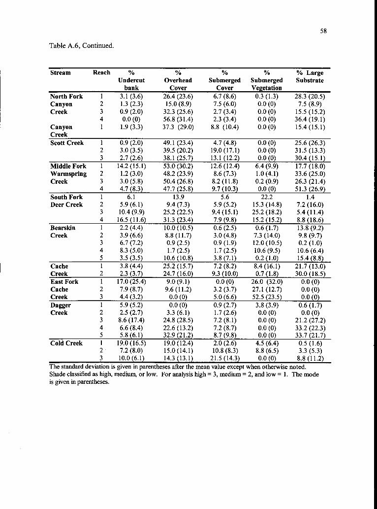
58

Table A.6, Continued.

Stream Reach %Undercut

bank

%Overhead

Cover

%Submerged

Cover

%SubmergedVegetation

% LargeSubstrate

North Fork 1 3.1 (3.6) 26.4 (23.6) 6.7 (8.6) 0.3 (1.3) 28.3 (20.5)Canyon 2 1.3 (2.3) 15.0 (8.9) 7.5 (6.0) 0.0 (0) 7.5 (8.9)Creek 3 0.9 (2.0) 32.3 (25.6) 2.7 (3.4) 0.0 (0) 15.5 (15.2)

4 0.0 (0) 56.8 (31.4) 2.3 (3.4) 0.0 (0) 36.4 (19.1)Canyon 1 1.9 (3.3) 37.3 (29.0) 8.8 (10.4) 0.0 (0) 15.4 (15.1)CreekScott Creek 1 0.9 (2.0) 49.1 (23.4) 4.7 (4.8) 0.0 (0) 25.6 (26.3)

2 3.0 (3.5) 39.5 (20.2) 19.0 (17.1) 0.0 (0) 31.5 (13.3)3 2.7 (2.6) 38.1 (25.7) 13.1 (12.2) 0.0 (0) 30.4 (15.1)

Middle Fork 1 14.2 (15.1) 53.0 (30.2) 12.6 (12.4) 6.4 (9.9) 17.7 (18.0)Warmspring 2 1.2 (3.0) 48.2 (23.9) 8.6 (7.3) 1.0 (4.1) 33.6 (25.0)Creek 3 3.0 (5.8) 50.4 (26.8) 8.2 (11.8) 0.2 (0.9) 26.3 (21.4)

4 4.7 (8.3) 47.7 (25.8) 9.7 (10.3) 0.0 (0) 51.3 (26.9)South Fork 1 6.1 13.9 5.6 22.2 1.4Deer Creek 2 5.9 (6.1) 9.4 (7.3) 5.9 (5.2) 15.3 (14.8) 7.2 (16.0)

3 10.4 (9.9) 25.2 (22.5) 9.4 (15.1) 25.2 (18.2) 5.4 (11.4)4 16.5 (11.6) 31.3 (23.4) 7.9 (9.8) 15.2 (15.2) 8.8 (18.6)

Bearskin 1 2.2 (4.4) 10.0 (10.5) 0.6 (2.5) 0.6 (1.7) 13.8 (9.2)Creek 2 3.9 (6.6) 8.8 (11.7) 3.0 (4.8) 7.3 (14.0) 9.8 (9.7)

3 6.7 (7.2) 0.9 (2.5) 0.9 (1.9) 12.0 (10.5) 0.2 (1.0)4 8.3 (5.0) 1.7 (2.5) 1.7 (2.5) 10.6 (9.5) 10.6 (6.4)5 3.5 (3.5) 10.6 (10.8) 3.8 (7.1) 0.2 (1.0) 15.4 (8.8)

Cache 1 3.8 (4.4) 25.2 (15.7) 7.2 (8.2) 8.4 (16.1) 21.7 (13.0)Creek 2 2.3 (3.7) 24.7 (16.0) 9.3 (10.0) 0.7 (1.8) 30.0 (18.5)East Fork 1 17.0 (25.4) 9.0 (9.1) 0.0 (0) 26.0 (32.0) 0.0 (0)Cache 2 7.9 (8.7) 9.6 (11.2) 3.2 (3.7) 27.1 (12.7) 0.0 (0)Creek 3 4.4 (3.2) 0.0 (0) 5.0 (6.6) 52.5 (23.5) 0.0 (0)Dagger 1 5.9 (5.2) 0.0 (0) 0.9 (2.7) 3.8 (3.9) 0.6 (1.7)Creek 2 2.5 (2.7) 3.3 (6.1) 1.7 (2.6) 0.0 (0) 0.0 (0)

3 8.6 (17.4) 24.8 (28.5) 7.2 (8.1) 0.0 (0) 21.2 (27.2)4 6.6 (8.4) 22.6 (13.2) 7.2 (8.7) 0.0 (0) 33.2 (22.3)5 5.8 (6.1) 32.9 (21.2) 8.7 (9.8) 0.0 (0) 33.7 (21.7)

Cold Creek 1 19.0 (16.5) 19.0 (12.4) 2.0 (2.6) 4.5 (6.4) 0.5 (1.6)2 7.2 (8.0) 15.0 (14.1) 10.8 (8.3) 8.8 (6.5) 3.3 (5.3)3 10.0 (6.1) 14.3 (13.1) 21.5 (14.3) 0.0 (0) 8.8 (11.2)

The standard deviation is given in parentheses after the mean value except when otherwise noted.Shade classified as high, medium, or low. For analysis high = 3, medium = 2, and low = 1. The modeis given in parentheses.

59

Table A.6, Continued.

Stream Reach % Mean %Bubble Shade OverstoryCover (Mode)*

North Fork Canyon 1 9.3 (9.5) 2.2 (2) 72.7 (17.9)Creek 2 5.0 (5.4) 2.4 (3) 63.1 (25.5)

3 10.0 (8.1) 2.7 (3) 83.5 (30.3)4 30.0 (23.2) 2.5 (2) 23.3 (31.3)

Canyon Creek 1 10.0 (15.4) 1.5 (1) 90.8 (6.4)Scott Creek 1 NA 2.0 (2) 28.5 (32.1)

2 NA 1.3 (1) 81.5 (22.4)3 NA 2.1 (2) 43.2 (37.8)

Middle Fork Warmspring 1 NA 2.7 (3) 69.7 (28.4)Creek 2 NA 2.0 (2) 37.3 (27.0)

3 NA 1.8 (2) 40.1 (37.7)4 NA 2.7 (3) 31.0 (32.7)

South Fork Deer Creek 1 NA 1.1 (1) 21.22 NA 1.9 (2) 64.4 (33.3)3 NA 1.4 (1) 28.6 (27.0)4 NA 1.7 (1) 19.8 (26.0)

Bearskin Creek 1 1.6 (3.0) 2.2 (2) 76.4 (14.3)2 0.9 (2.4) 2.1 (2) 66.5 (13.0)3 0.0 (0) 1.3 (1) 38.7 (27.5)4 0.6 (1.7) 2.1 (2) 90.0 (8.5)5 4.4 (6.1) 2.3 (2) 92.1 (8.1)

Cache Creek 1 3.6 (6.8) 2.3 (3) 61.3 (38.1)2 12.3 (13.9) 2.6 (3) 70.3 (31.6)

East Fork Cache Creek 1 0.5 (1.6) 1.1 (1) 27.5 (20.5)2 2.5 (8.0) 1.0 (1) 92.5 (3.4)3 0.0 (0) 1.1 (1) 57.5 (42.7)

Dagger Creek 1 0.0 (0) 1.3 (1) 25.0 (44.7)2 0.8 (2.0) 1.2 (1) 41.7 (49.2)3 NA 2.4 (2) 59.8 (31.9)4 NA 1.7 (2) 75.5 (34.7)5 NA 2.7 (3) 81.7 (25.8)

Cold Creek 1 0.0 (0) 1.5 (1) 10.0 (29.9)2 2.5 (8.3) 2.7 (3) 84.3 (25.5)3 6.8 (13.6) 2.6 (3) 99.2 (2.5)

60

Table A.7. Summary of fish densities in reaches.

Stream Reach Total Bull Total Bull Total BullTrout Trout per Trout <

100 m2 140 mm

Total BullTrout < 140mm per 100

m2

Total BullTrout > 140

mm

Total BullTrout >

140mm per100 M2

North Fork 1 238 2.40 165 1.67 73 0.74Canyon 2 45 4.48 43 4.28 2 0.20Creek 3 106 4.33 43 1.76 63 2.57

4 58 2.82 18 0.88 40 1.95Canyon 1 120 1.77 53 0.78 67 0.99CreekScott Cr. 1 65 1.41 23 0.50 42 0.91

2 4 0.60 0 0.00 4 0.603 6 0.84 4 0.56 2 0.28

Middle Fork 1 32 0.98 27 0.83 5 0.15Warmspring 2 49 2.00 47 1.92 2 0.08Creek 3 86 2.72 84 2.66 2 0.06

4 39 2.46 36 2.27 3 0.19South Fork 1 0 0.00 0 0.00 0 0.00Deer Creek 2 1 0.04 1 0.04 0 0.00

3 63 1.81 62 1.78 1 0.034 5 0.60 5 0.60 0 0.00

Bearskin 1 42 1.14 40 1.08 2 0.05Creek 2 66 1.78 62 1.67 4 0.11

3 31 1.19 29 1.11 2 0.084 41 4.68 36 4.11 5 0.575 50 2.50 42 2.10 8 0.40

Cache Creek 1 3 0.08 3 0.08 0 0.002 3 0.13 3 0.13 0 0.00

East Fork 1 15 2.59 11 1.90 4 0.69Cache Creek 2 19 3.97 13 2.72 6 1.25

3 1 0.12 1 0.12 0 0.00Dagger 1 18 1.17 14 0.91 4 0.26Creek 2 22 2.35 14 1.50 8 0.86

3 22 0.88 22 0.88 0 0.004 43 3.16 40 2.94 3 0.225 32 2.55 29 2.31 3 0.24

Cold Creek 1 13 2.08 13 2.08 0 0.002 21 1.18 18 1.01 3 0.173 20 1.70 17 1.44 3 0.25

61

Table A.7, Continued.

Stream Reach TotalRainbow

Trout

Total RainbowTrout per 100 m2

Total BrookTrout

Total BrookTrout per 100 m2

North Fork 1 6 0.06 1 0.01Canyon 2 0 0.00 0 0.00Creek 3 19 0.78 0 0.00

4 31 1.51 0 0.00Canyon Creek 1 15 0.22 0 0.00Scott Cr. 1 0 0.00 0 0.00

2 0 0.00 0 0.003 0 0.00 0 0.00

Middle Fork 1 28 0.86 0 0.00Warmspring 2 5 0.20 0 0.00Creek 3 0 0.00 0 0.00

4 0 0.00 0 0.00South Fork 1 78 2.92 0 0.00Deer Creek 2 58 2.42 0 0.00

3 38 1.09 0 0.004 3 0.36 0 0.00

Bearskin 1 1 0.03 19 0.51Creek 2 0 0.00 24 0.65

3 0 0.00 5 0.194 0 0.00 2 0.235 0 0.00 0 0.00

Cache Creek 1 150 4.23 18 0.512 193 8.29 3 0.13

East Fork 1 0 0.00 5 0.86Cache Creek 2 0 0.00 2 0.42

3 0 0.00 2 0.25Dagger 1 23 1.49 0 0.00Creek 2 23 2.46 0 0.00

3 62 2.49 0 0.004 49 3.60 0 0.005 14 1.12 0 0.00

Cold Creek 1 0 0.00 0 0.002 1 0.06 0 0.003 1 0.08 1 0.08

62

Table A.8. Summary of habitat characteristics in patches.

Stream Gradient MeanElevation

(m)

Daily Mean Daily TotalMean Maximum HabitatTemp. Temp. (°C) Units

Total#

Pools

%

PoolsPools

per 100 m

(°C)North ForkCanyonCreek

8.4 1947 7.5 9.1 303 156 51.5 4.3

Scott Creek 4.4 1917 6.3 8.2 191 86 45.0 4.4Middle ForkWarmspringCreek

6.8 1878 7.5 9.0 462 251 54.3 7.0

South ForkDeer Creek*

1.4 2046 8.2 11.2 473 312 66.0 8.8

BearskinCreek

4.6 2062 7.7 9.8 413 256 62.0 5.4

Cache Creek 4.1 2109 9.2 10.9 202 111 55.0 7.4Dagger Creek 4.4 2023 8.1 10.3 317 206 65.0 10.1

East ForkCache Creek

1.0 2165 7.7 10.7 114 66 57.9 6.8

Cold Creek 0.5 1968 7.5 9.6 209 119 56.9 7.4*Values do not include reach 1 of South Fork Deer Creek.

Table A.8, Continued.

Stream TotalLength (m)

Mean UnitLength (m)

Mean UnitWidth (m)

Mean Unit Depth(m)

North Fork Canyon Creek 4481.1 13.18 (18.03) 4.44 (1.97) 0.21 (0.09)Scott Creek 1942.5 10.73 (13.3) 2.94 (0.91) 0.13 (0.07)Middle Fork WarmspringCreek

3564.4 7.61 (7.97) 2.96 (0.84) 0.17 (0.07)

South Fork Deer Creek* 2782.6 7.13 (4.85) 2.26 (0.95) 0.18 (0.06)Bearskin Creek 4763.9 11.53 (14.12) 2.63 (0.85) 0.23 (0.11)Cache Creek 1506.9 7.46 (8.16) 3.92 (1.28) 0.16 (0.05)Dagger Creek 2031.6 7.48 (6.22) 2.38 (0.77) 0.17 (0.05)East Fork Cache Creek 976.7 8.57 (8.75) 1.90 (1.05) 0.26 (0.16)Cold Creek 1599.1 7.65 (7.00) 2.26 (0.72) 0.16 (0.06)

The standard deviation is given*Values do not include reach 1

in parentheses after the mean value.of South Fork Deer Creek.

63

Table A.8, Continued

Stream Mean PoolMax.

Depth (m)

Mean Pool CrestDepth (m)

Width:DepthRatio

Width:Max.

Depth RatioNorth Fork Canyon Creek 0.60 (0.17) 0.22 (0.08) 21.14 7.4Scott Creek 0.46 (0.18) 0.17 (0.11) 24.40 6.32Middle Fork WarmspringCreek

0.43 (0.09) 0.21 (0.08) 17.44 6.84

South Fork Deer Creek* 0.42 (0.11) 0.20 (0.08) 11.97 5.72Bearskin Creek 0.49 (0.14) 0.16 (0.06) 11.19 5.43Cache Creek 0.48 (0.12) 0.14 (0.06) 24.79 7.68Dagger Creek 0.46 (0.12) 0.16 (0.06) 13.76 5.77East Fork Cache Creek 0.61 (0.20) 0.15 (0.09) 7.39 3.11Cold Creek 0.40 (0.09) 0.14 (0.06) 12.60 5.66

Table A.8, Continued.

Stream ResidualPool

Depth (m)

PocketPools per

100 m

MeanDepth ofPocket

Pools (m)

MeanDominateSubstrate(Mode)*

MeanSubdominant

Substrate(Mode)*

Surfacefines

Stablebank

North ForkCanyon Creek

0.38 39.9 0.28 4.4 (4) 4.1 (4) 8 (7.2) 97 (9.4)

Scott Creek 0.30 11.2 0.24 4.1 (5) 3.0 (1) 22 (13.9) 86 (18.8)Middle ForkWarmspringCreek

0.20 11.2 0.28 4.0 (2) 3.9 (3) 26 (17.9) 97 (8.9)

South ForkDeer Creek*

0.20 1.2 0.27 2.7 (5) 2.1 (1) 39 (27.4) 95 (7.6)

BearskinCreek

0.32 5.37 0.49 3.5 (3) 2.9 (2) 12 (9.2) 97 (5.3)

Cache Creek 0.37 14.7 0.29 3.9 (4) 3.4 (3) 21 (20.8) 97 (9.9)Dagger Creek 0.24 10.3 0.25 4.1 (5) 3.7 (4) 23 (18.1) 83 (21.3)East ForkCache Creek

0.46 3.4 0.27 1.9 (2) 2.1 (3) 22 (17.1) 89 (11.6)

Cold Creek 0.25 5.1 0.30 1.6 (1) 2.4 (3) 58 (27.2) 86 (19.8)The standard deviation is given in parentheses after the mean value except when otherwise noted.*Values do not include reach 1 of South Fork Deer Creek.

64

Table A.8 Continued.

Stream LargeWoodyDebris

(Singles)per 100 m2

Total Large Total Large Total LargeWoody Woody WoodyDebris Debris Debris

Aggregates per 100 m2 (pieces) perper 100 m 100m

Lateral MeanHabitat Shade

Areas per (Mode)*100 m

Overstory

North ForkCanyonCreek

7.9 5.3 13.4 34.8 14.4 2.2 (2) 68 (30.6)

Scott Creek 6.3 3.1 9.9 NA 0.9 1.8 (3) 43 (37.6)Middle ForkWarmspringCreek

13.7 13.2 29.9 NA 1.0 2.3 (2) 47 (34.9)

South ForkDeer Creek*

8.8 5.1 14.3 NA 1.5 1.5 (1) 33 (31.7)

BearskinCreek

6.2 3.90 10.20 20.36 10.41 2.0 (2) 70 (25.5)

Cache Creek 10.7 8.4 19.2 61.4 3.7 2.4 (3) 65 (35.7)Dagger Creek 18.1 11.4 30.1 NA 1.3 2.3 (2) 61 (39.6)East ForkCache Creek

7.5 1.6 9.1 11.8 6.6 1.1 (1) 62 (37.1)

Cold Creek 10.9 12.3 23.8 72.2 4.7 2.4 (3) 75 (39.3)The standard deviation is given in parentheses after the mean value except when otherwise noted.*Values do not include reach 1 of South Fork Deer Creek.

Table A.8, Continued.

StreamUndercut

bank

°A)

OverheadCover

%Submerged

Cover

% LargeSubmerged SubstrateVegetation

%BubbleCover

North Fork CanyonCreek

1.9 (3.1) 32.6 (27.3) 5.9 (7.8) 0.1 (0.8) 22.9 (19.5) 12.2(15.0)

Scott Creek 2.0 (2.7) 43.1 (23.4) 11.0 (12.6) 0.0 (0) 28.6 (2) NAMiddle ForkWarmspring Creek

6.5 (11.2) 50.3 (26.9) 10.0 (10.9) 2.4 (6.6) 29.0 (24.6) NA

South Fork DeerCreek*

11.2 (10.5) 24.1 (22.0) 8.5 (12.5) 20.5 (17.2) 6.7 (14.5) NA

Bearskin Creek 4.6 (5.9) 7.0 (10.0) 2.2 (4.7) 5.9 (10.5) 9.7 (9.6) 1.6 (3.8)Cache Creek 3.3 (4.2) 25.0 (15.6) 8.0 (8.8) 5.8 (13.6) 24.5 (15.4) 6.6

(10.6)Dagger Creek 6.6 (10.7) 20.1 (22.1) 6.0 (8.1) 0.7 (2.1) 22.1 (24.5) NAEast Fork Cache Creek 9.8 (15.7) 7.0 (9.7) 2.7 (4.4) 33.1 (24.8) 0.0 (0) 1.3 (5.4)Cold Creek 10.5 (10.3) 15.5 (13.3) 13.1 (12.5) 4.7 (6.4) 4.8 (8.2) 3.6

(10.2)The standard deviation is given in parentheses after the mean value.*Values do not include reach 1 of South Fork Deer Creek.

65

Table A.9. Summary of fish densities in patches.

Stream TotalBull

Trout

Total Bull Total BullTrout per Trout

100 m2 < 140 mm

Total BullTrout 5_ 140

mm per 100 m2

Total BullTrout >140 mm

Total BullTrout > 140

mm per 100 m2North ForkCanyon Creek

449.00 3.22 271.00 1.94 178.00 1.27

Scott Creek 75.00 1.38 27.00 0.50 48.00 0.88Middle ForkWarmpring Creek

206.00 1.95 194.00 1.84 12.00 0.11

South Fork DeerCreek

69.00 0.72 68.00 0.71 1.00 0.01

Bearskin Creek 230.00 1.83 209.00 1.67 22.00 0.18Cache Creek 6.00 0.10 6.00 0.10 0.00 0.00East Fork CacheCreek

35.00 1.88 25.00 1.34 10.00 0.54

Dagger Creek 97.00 1.92 91.00 1.80 6.00 0.12Cold Creek 54.00 1.49 48.00 1.33 6.00 0.17

Table A.9, Continued.

Stream TotalRainbow

Trout

Total RainbowTrout per 100 m2

Total BrookTrout

Total Brook Troutper 100 m2

North Fork CanyonCreek

56.00 0.40 1.00 0.01

Scott Creek 0.00 0.00 0.00 0.00Middle Fork WarmpringCreek

33.00 0.31 0.00 0.00

South Fork Deer Creek 177.00 1.86 0.00 0.00Bearskin Creek 1.00 0.01 50.00 0.40Cache Creek 343.00 5.81 21.00 0.36East Fork Cache Creek 0.00 0.00 9.00 0.48Dagger Creek 124.00 2.45 0.00 0.00Cold Creek 2.00 0.06 1.00 0.03