REDEFINING HONEYBEE FORAGING COGNITION

BY

Daniel A. Najera

Submitted to the Department of Ecology and Evolutionary Biology of the University of Kansas

in partial fulfillment of the requirements for the degree of Doctor of Philosophy

_____________________________ ___________ Rudolf Jander Date

_____________________________ ___________ Orley R. Taylor Jr. Date

_____________________________ ___________ Deborah Smith Date

_____________________________ ___________ Bryan L. Foster Date

_____________________________ ___________ Ann E. Cudd Date

The Dissertation Committee for Daniel A. Najera certifies that this is the approved version of the following dissertation

“Redefining Honeybee Foraging Cognition”

The University of Kansas – Spring 2009

___________________________ _____ Rudolf Jander Date

___________________________ _____ Orley R. Taylor Jr. Date

___________________________ _____ Deborah Smith Date

___________________________ _____ Bryan L. Foster Date

___________________________ _____ Ann E. Cudd Date

2

Table of Contents

Abstract – page 6

Chapter 1 – Introduction and Method – page 7 -The Beloved Honeybee -Beyond the Dance -Interpatch Foraging -Our New Method

Study 1 - “Redefining Honeybee Spatial Cognition: Refined Concepts and Novel Experimental Methods”

Chapter 2 – Investigating Landmark Theory – page 31 -Background -Problems with Previous Experiments

Study 2 - “The Interpatch Path – How honeybees choose a direction” Chapter 3 – Challenging Landmark Theory – page 45 -Experimental Power -Manipulation of Experimental Design

Study 3 - “Knowing the path: Interpatch Decision Making in Honeybees without Terrestrial Cues”

-Independence of Terrestrial Cues Chapter 4 – Investigating Route Theory – page 55 -Route Knowledge -Training Sequence Knowledge

Study 4 - “The Traveling Salesman meets the Traveling Consumer: Sequence Understanding and Extrapolation in Honeybees (Apis mellifera)

-When the Rules Change Chapter 5 – Challenging Route Theory – page 66 -How to Challenge Route Theory -The Hive as a Hub -Secondary Hubs -Stimulus Dependent Decision Making Outside of the Hive

3

Study 5 - “Secondary Hubs in Honeybees: Demonstration of Branching Interpatch Decision Making”

-Initial Tests: Long-Term Memory vs. Short-Term Memory

-Finishing Direction Knowledge Chapter 6 – The Quest for Distance Knowledge – page 86 -A New Method -How to Subtract Utility

Study 6 - “The shortest path between two points: Interpatch Distance Knowledge in Honeybees (Apis mellifera)”

-Finishing Distance Knowledge Chapter 7 – Investigating Shortcut Making – page 101 -The Shortcut -The Place Map -Displacement vs. No Displacement -Ecological Utility for Motivation

Study 7 - “Generation of Novel Shortcut Interpatch Paths Using Realistic, Ecologically Based Motivations in the Honeybee (Apis mellifera)”

-Producing Shortcuts -Where to Go Next Chapter 8 – Challenging the Honeybee – page 110 -Complexity – Is it a game? -Simultaneous Manipulation of Information

Study 8 - “Logic in Honeybees (Apis mellifera); Demonstration of conditional, syllogistic reasoning in the context of foraging.”

-Six Dimensional Decision Making Chapter 9 – Summary of Research – page 122 -A New Perspective -The Recent Failure of the Cognitive Map -The Utility of the Place Map -Impact on Previous Theory -The Place Map and Additions -Pushing the Limits

4

-The Beloved Honeybee – Revisited Literature Cited – page 127

5

Abstract for the Dissertation of

Daniel A. Najera

“Redefining Honeybee Foraging Cognition” The research in this manuscript was designed to investigate all of the facets of current honeybee foraging knowledge. In order to do so, we constructed new methodologies to provide more accurate data for a finer level of analysis. Specifically, we were able to quantify horizontal and vertical directions of departure, using immediate decision making. Also, we were able to test complete vector knowledge of flown paths with distance methods as well, relying upon the subtraction of utility for cues other than distance. We then conclude that landmark, route, and cognitive map theories are only parts to a complex cognitive system. In this complex cognitive system resides the ability to logically deduce specific foraging strategies, representing a network of cognitive systems used for decision making. The mind of the honeybee is likely harboring more cognitive abilities than we were able to discover.

6

Chapter 1

Introduction and Method The Beloved Honeybee

The beloved honeybee is one of the most commonly encountered organisms on the planet. Across the world, honeybees provide services for humanity. In nearly all agricultural communities, one can see the white painted Langstroth boxes littering the landscape. On picnics or near ornamental flowers, one can often glimpse multiple honeybees. The entertainment industry has also found these organisms of interest by adapting various honeybee cartoon symbols with positive connotations; the honeybee is one of the rare insects that makes people smile. It is easy to say the honeybee is one of our likable organisms. It is also easy to say the products of the honeybee colony are quite likable by humans as well. Honey is used all over the world as a sweetener especially where sugarcane is not easily available. The wax itself is also used for a variety of applications, as well as the “beebread” (mainly pollen). All of these products are well known, but there is so much more to know that often goes untold. Following Karl Von Frisch’s discovery of the honeybee dance communications (1967), the discipline of Ethology was forever transformed. The general public, unfortunately, is not aware of these dances or the communicative information they convey. Even for that rare subset of the population that does know about these dances, they often do not know what else Von Frisch discovered with bees. This research includes many perceptual qualifications and quantifications, including the first demonstration of color vision in any non-human animal (Von Frisch 1914/1915).

With all the information from Von Frisch and the research on honeybee culture (societal organization), the honeybee became quite well understood. The level of cognition of honeybees was greatly expanded and people began to use these dances as an investigational entry point into the mind of the bee. Unfortunately, the dances were so amazing they began to define the bee. They were simultaneously the answer to foraging questions (Von Frisch 1967), circadian rhythm questions (Bogdany 1978, Dyer 1987), as well as genetic questions (Robinson et al. 2008). They were even used to describe the evolution of honeybees in general, including some aspects of their society and social cognition (Robinson et al. 2008). It is now time to step back from the dances to regain perspective.

The dance, no matter how spectacular it is, is a mechanism for communication. In no known communication is there 100% transmission of information (Shannon 1948); some semiconducting computers may be exceptions, but definitely no examples from biological communication. This means the dance observer cannot exactly obtain the information from the dancer; it is often good enough, of course. Also, the information the dancer knows about the location cannot be encoded into the dance at 100% efficiency. Therefore, the dance itself is at best a

7

skewed representation of what is in the mind of the dancing honeybee. We know a great deal about the information they can communicate, but what has not been answered are questions about the complete knowledge of the bee.

What is in the mind of a bee? No research on honeybees has ever come as close to answering this question as the research contained in this manuscript. In fact, through this research, it becomes quite apparent how far from answering this question we are. To sufficiently answer this question, we must remove our self from the largest constraining obstacle, the dances themselves.

Beyond the Dance To gain the correct perspective, we need a thought provoking question, “Which came first, the dance or the intelligence.” There are those who would argue for the dance. Opposing them would be those in favor of intelligence. Even still, another group would say it was interactive and things co-evolved. We need not debate this question here, but only use it to intrigue ourselves so we can adequately understand the sequence of events which lead to the research in this manuscript. If one believes, as the majority of all people do (even biologists), that insects are stupid and incapable of intelligence, then the dance MUST be the pinnacle of their intelligence; these humans are unwilling to assume more. This perspective could easily lead to one of the following two paths of reasoning. One might say the energy from resources excited honeybees so they started moving more (dances first) then the intelligence evolved to understand it. One might say honeybees made locomotion more and more informative as they became more and more intelligent (co-evolving). Their maximized intelligence is then manifested in the dance. Either way, after at least 50 million years (Michener and Grimaldi 1988) this dance is the extent of their knowledge. If one believes that brains are brains and no matter where you find them, intelligence can be found; there is nothing special about human skulls or exoskeleton compartments. We must admit that we have next to no predictive ability when it comes to knowing how many neurons an organism needs, or how a neural network needs to be arranged for an organism understand any qualitative concepts like home, food, location, time, numbers, logic, self, etc. Honeybees have roughly one million neurons and we are unable to exclude the possibility of any of these concepts (or any degree of high level intelligence) based upon observable data. With this perspective, the dance need not be the pinnacle of honeybee intelligence. In fact, it could be that the honeybee is far more intelligent and their morphology constrains their ability to communicate the full capacity of concepts in their brain (intelligence first). An easy way for humans to understand such constraint is to recall a time when your own super communication (human language) failed you. These are the times when you had to tell someone, “I can’t find the words” or “I don’t know how to describe it” even when you had the knowledge in your head. No communication is 100% efficient, not even ours. In addition, given this perspective, it would then be accepted that the dances are one expression of the mind of honeybees, not the definition of their limitations.

8

With this perspective, we can hypothesize that the knowledge of the honeybee is greater than the information contained in the dance; based upon our data, it is far greater than previously imagined. We cannot look at the dance for answers as it is a poor representation of their cognitive abilities. If we survey the honeybee literature, we come up with a dismal amount of research harboring this perspective. Nearly everything we find relates concepts back to dance performance or information that could be obtained from the dances. We must remove ourselves from the dances to see clearly and we do so in the following way. Interpatch Foraging Foraging can be defined as the search for and acquisition of food. It is one of the most consistent and demanding tasks for any given living organism. It is directly related to the survivability of the organism in that poor foragers have lower survivability. On the other hand, to be a good forager, you must be well informed about your food or lucky. Such foraging information consists of locations, distances between locations, and the availability of food (spatial and temporal abundance as well as quality).

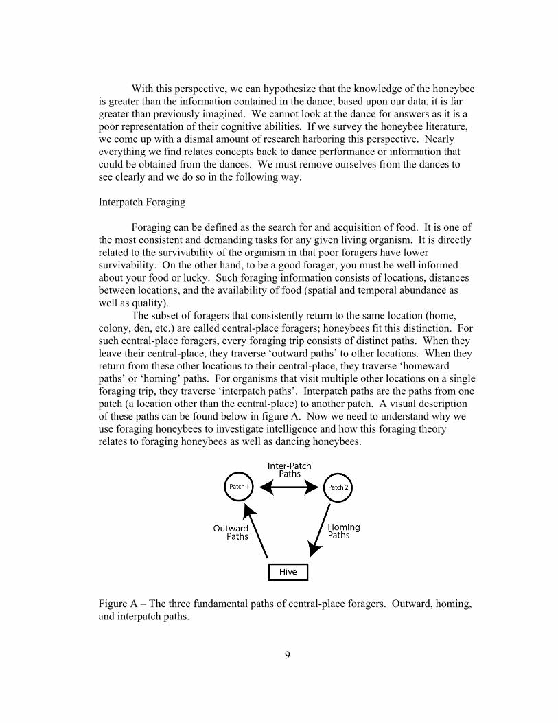
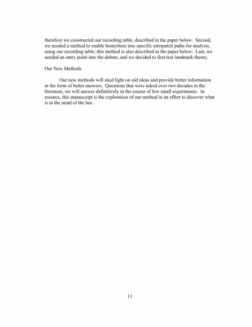
The subset of foragers that consistently return to the same location (home, colony, den, etc.) are called central-place foragers; honeybees fit this distinction. For such central-place foragers, every foraging trip consists of distinct paths. When they leave their central-place, they traverse ‘outward paths’ to other locations. When they return from these other locations to their central-place, they traverse ‘homeward paths’ or ‘homing’ paths. For organisms that visit multiple other locations on a single foraging trip, they traverse ‘interpatch paths’. Interpatch paths are the paths from one patch (a location other than the central-place) to another patch. A visual description of these paths can be found below in figure A. Now we need to understand why we use foraging honeybees to investigate intelligence and how this foraging theory relates to foraging honeybees as well as dancing honeybees.

Figure A – The three fundamental paths of central-place foragers. Outward, homing, and interpatch paths.

9

How good are honeybee foragers? Honeybee foragers are so efficient we can commercially exploit them with little maintenance. One can literally put a Langstroth colony down and at the end of the year expect at least 20 lbs of honey; if managed properly (little maintenance), to upwards of 120 lbs of honey. This honey is the result of millions and millions of foraging trips to flowers of many species that vary widely in floral characteristics, both within and between species. On a single foraging trip a honeybee can often visit 10s or 100s of flowers of potentially different species, foraging on both pollen and nectar simultaneously. With respect to such foraging paths, there is only one outward path, only one homeward path, and many interpatch paths (depending on how you spatially/temporally define a patch).

With such complex food resources and foraging paths, we expect they will have complex intelligence to understand them. If we are to investigate their intelligence adequately we must separate ourselves from the dance. With these three component paths (outward, homing, and interpatch) we need to investigate the influence of the dances on these paths, or the influence of the paths on these dances, depending on one’s perspective.

It has been shown that dances can contain information from the whole roundtrip (outward and homeward paths) (Von Frisch 1967); therefore these were lower in priority to investigate. It has never been shown that information from the interpatch path has been conveyed by the dances, but it has been attempted (Tanner and Visscher 2006); therefore this path was much higher in priority to investigate. When surveying the literature of research on interpatch paths, again it is dismal, but there were some starting points.

Interpatch foraging theory in 2004 (when I began graduate school) was based upon few experiments, of which none adequately controlled the sources of information used by the honeybees during their experiments. Most relied on information from outward and homing paths, however, research has produced three leading hypotheses: landmark theory, route theory, and cognitive map theory. Through the course of this manuscript, we will deal with each.

Landmark theory basically stated that in order to travel from one patch to another, honeybees would rely on conspicuous terrestrial features. The leading promoters of this theory at the time were (Cartwright, B. A. and Collett, T.S.); we discuss this theory in chapters 2 and 3. Route theory basically stated that honeybees would know a single route that would take them to multiple places in a sequential one-dimensional (non-branching) fashion. They were constrained in their foraging path by the routes they had decided in the colony. The leading promoters were (Dyer, F. C., Cheng, K., Wehner, R. and Wehner, S, Menzel, R.); we discuss this theory in chapters 4 and 5. Cognitive map theory basically stated that honeybees could compute the distance and direction from one patch to the other and decide which path to take at any time. The leading promoters were (Gould, J. L.); we discuss this theory in chapters 6 and 7. We decided to join the fun, but needed a new way to look at these theories.

First, we needed a new method that would adequately control for all the sources of information used by honeybees, specifically during decision making;

10

therefore we constructed our recording table, described in the paper below. Second, we needed a method to enable honeybees into specific interpatch paths for analysis, using our recording table; this method is also described in the paper below. Last, we needed an entry point into the debate, and we decided to first test landmark theory. Our New Methods Our new methods will shed light on old ideas and provide better information in the form of better answers. Questions that were asked over two decades in the literature, we will answer definitively in the course of few small experiments. In essence, this manuscript is the exploration of our method in an effort to discover what is in the mind of the bee.

11

Redefining Honeybee Spatial Cognition: Refined Concepts and Novel Experimental Methods

Danny A. Najera, Rudolf Jander

INTRODUCTION

With the goal of truly understanding the honeybee’s (Apis mellifera) complex navigational mechanisms, we have refined the involved concepts and devised novel experimental methods. All animals that efficiently find their way from place to place within their home range do so with the help of some mental (cognitive) representation, which is variously called the topographic, spatial, or cognitive map. However, the published definitions of these presumed synonymous terms vary widely (Tolman 1948, Bennett 1996, Healy et al. 2003, Foo et al. 2005). These underlying conceptual disparities are further confounded in honeybee literature by incomplete knowledge of the their navigational strategies, providing fertile ground for lively controversies (e.g. Collett 1987, Dyer 1991, Gallistel 1989, Gould 1986, Menzel et al. 2001, Kirchner and Braun 1994, Wehner and Menzel 1990), to the extent of complete reversals of opinion (Menzel et al. 1990 and Menzel et al. 2005). Here, we propose a consensus concept of place mapping as a simple solution for the "cognitive map controversies." A refined concept demands simplicity and consensus, which converge on the same concept. Simplicity requires us to identify the necessary, but minimal, criteria for our place mapping concept as such a simple map must have been the evolutionary starting point for subsequent elaboration. Consensus requires us to identify shared constituents of all previous concepts of mapping. By paring off the extra-consensus components we effectively eliminate any justification for deconstructive argumentation. In addition, each component of the place map is defined based upon data, resulting in a non-speculative and concise definition. The result is given below.

A REFINED CONCEPT – PLACE MAPPING We stipulate that animal minds incorporate place maps if they can mentally represent and recall two or more places and link them with topomotor route knowledge (used for dead reckoning), or more abstractly, spatial vector knowledge. This place map is the rudimentary foundation on which complexity can arise. The recall of places is activated by place-specific cues (e.g. landmarks); topomotor route knowledge is represented by the sensorimotor instructions used to navigate from one place to another. Such a place map is acquired (latently learned) through exploratory behavior, utilizing extensive place recognition learning and/or path-integration computations. Place recognition learning allows an organism to characterize and represent places as unique and distinct. Path-integration involves the computation of resultant vectors (displacement vectors) by integrating all vector elements (distance and direction) while moving from place to place (Jander 1957; Maurer & Sequinot

12

1995; Benhamou & Sequinot 1995). Given this simple and consensus definition of the place map, we first demonstrate its practical and logical application to honeybees using the classical research data of Karl von Frisch and collaborators (1967). There is ample evidence that individual honeybees recognize multiple places and that they know distances and directions from their hive to various feeding locations (Von Frisch 1967)—these two sets of facts perfectly meet our minimal criteria for place mapping. In addition, classical experiments demonstrate three more advanced place mapping skills. First, the honeybee’s place map incorporates all three dimensions of space (Von Frisch 1967, pp.253-255), one more than the conventional human map. Second, honeybees link spatial mapping with temporal mapping (Von Frisch 1967, pp.253-255). Therefore, we can speak of a 3-D-spatio-temporal place map. Third, honeybees have unambiguously been shown to compute novel vector directions between places using the experience of detour routes (shortcuts); this computation involves a geometric-deductive process that can be obtained by path integration (Von Frisch 1967, pp.173-183). Therefore, the place map is verified as being path integrateable (from hive to feeder) in addition to the above distinctions. Later, a compilation of additions can be made based upon other recent research.

THE NEED FOR NOVEL EXPERIMENTAL METHODS In the classical research, as well as much recent research, the honeybee’s dance communication proved to be a powerful and essential tool for understanding home-range orientation. These dances are now a fundamental constraint to progressing our knowledge of home-range orientation beyond what it is now; this constraint is evident for the following reasons. In their dances, bees communicate distances and directions only between their hive and one other location, and only in two-dimensional space. Yet, on a single journey a foraging bee may visit several different places while traveling in three-dimensional space. In such a journey, we can distinguish three major types of constituent flight paths: outward paths (hive to resource), homeward paths (resource to hive), and interpatch paths (resource to resource). Figure 1 diagrams these three fundamental foraging paths. The interpatch path is not represented in the dance language and at present, we have only the most rudimentary insight into what navigational skills bees may apply to interpatch foraging. In terms of honeybee intelligence, it is theoretically the most interesting foraging path for quantifying and qualifying cognitive understanding. Therefore, we must extend our experimental designs to incorporate such interpatch paths, beyond the constraints of the dance. We already know that the honeybees’ cognitive abilities are more complex than the dances convey.

13

Figure 1 – The three fundamental foraging paths. Outward path (H to 1), Homing path (2 to H) and the interpatch paths (1 to 2, 2 to 1). The interpatch path is much less studied.

Given the above definition of place mapping and what is known about the complex flight patterns of naturally foraging bees, a set of almost completely unanswered questions arise: Do honeybees remember, recognize, and localize the locations of multiple food patches they visit on a single trip? If so, what recognition cues do they use to differentiate them? What information is used to guide the departures of an interpatch flight and what measures do they use to link places together? Do bees know what routes to fly in three-dimensional space when flying from food source to food source? Here we present simple, efficient, and novel experimental designs and procedures, superior to all previously applied methods, to answer each of these intriguing questions and many others.

RESEARCH TOOLS AND METHODS Enabling Interpatch Flights

With proper reward schemes honeybees easily learn to fly consistently among different discrete feeding sites (patches). Therefore, we can analyze the behavior of the honeybees as they leave one feeding site for the other (interpatch foraging). Training begins as in Von Frisch (1967) with a feeder (sugar water) incrementally moved from the hive to the first feeding location (Fig. 2a). When the bees are familiar with this first location, we place a second feeder (water only) as close as possible to the first feeder (Fig. 2b). Food availability is then alternated by switching the feeders. Then, while continually alternating food availability at the first and second feeder we incrementally move the second feeder to its final destination (Fig. 2c). The honeybees easily learn to make beelines to the respective other feeder if food is unavailable at that particular location; interpatch distances have reached up to 150 m, with no attempts to extend past this distance.

14

Figure 2 – Enabling interpatch flights. a) Incremental training to location 1. b) Introduction of feeder 2. c) Incremental training to location 2. Food availability is alternated between location 1 and two the entire time. The square with H represents the hive, while the two numbered circles represent feeding locations.

Experimental Designs for Recording Navigation Vectors

To make a beeline from place to place the honeybee’s underlying vector knowledge may cover values in three independent (orthogonal) parameters: two directional (horizontal and vertical) and one distal value. We have developed techniques to quantify the behavioral expressions of these three memories. Here we present the experimental designs to capture directional knowledge as expressed by departure directions.

Horizontal Direction of Departure To determine departure directions in the horizontal plane we surround a feeder at a distance of 50cm with 12 equally spaced vertical steel rods (3 mm thick, Fig.3a). By recording which of the 12 sectors bees depart through, we collect discrete data in 12, 30 degree categories.

Vertical Direction of Departure To distinguish between vertical and horizontal departures we place a square canvas (1.5 x 1.5m) 1m away from the feeder (Fig. 3b). Behind the screen we used a modified flag pole to elevate the feeder 5m above the feeding table. While viewing the feeder with the screen in the background, it proved simple to determine whether a departing bee crosses the upper, the left or the right margin of the screen; this screen provides discrete data of 3 sectors.

15

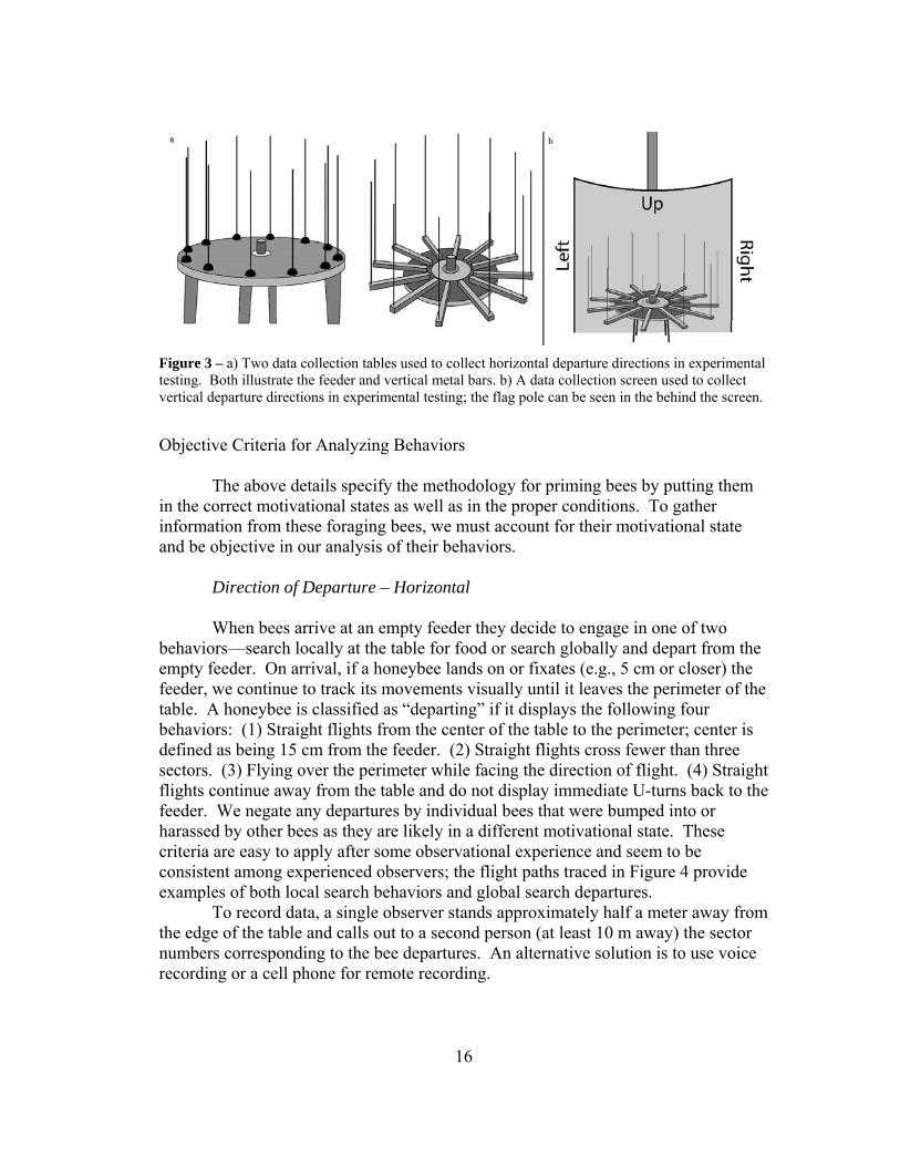
Figure 3 – a) Two data collection tables used to collect horizontal departure directions in experimental testing. Both illustrate the feeder and vertical metal bars. b) A data collection screen used to collect vertical departure directions in experimental testing; the flag pole can be seen in the behind the screen.

Objective Criteria for Analyzing Behaviors

The above details specify the methodology for priming bees by putting them in the correct motivational states as well as in the proper conditions. To gather information from these foraging bees, we must account for their motivational state and be objective in our analysis of their behaviors.

Direction of Departure – Horizontal When bees arrive at an empty feeder they decide to engage in one of two behaviors—search locally at the table for food or search globally and depart from the empty feeder. On arrival, if a honeybee lands on or fixates (e.g., 5 cm or closer) the feeder, we continue to track its movements visually until it leaves the perimeter of the table. A honeybee is classified as “departing” if it displays the following four behaviors: (1) Straight flights from the center of the table to the perimeter; center is defined as being 15 cm from the feeder. (2) Straight flights cross fewer than three sectors. (3) Flying over the perimeter while facing the direction of flight. (4) Straight flights continue away from the table and do not display immediate U-turns back to the feeder. We negate any departures by individual bees that were bumped into or harassed by other bees as they are likely in a different motivational state. These criteria are easy to apply after some observational experience and seem to be consistent among experienced observers; the flight paths traced in Figure 4 provide examples of both local search behaviors and global search departures. To record data, a single observer stands approximately half a meter away from the edge of the table and calls out to a second person (at least 10 m away) the sector numbers corresponding to the bee departures. An alternative solution is to use voice recording or a cell phone for remote recording.

16

Figure 4 – Traced flight paths of honeybees in horizontal direction of departure experiments; a) Homeward departures, b) Interpatch departures, and c) Non-departing, locally searching bees.

Direction of Departure – Vertical

The objective criteria used in horizontal departures is the same as vertical. However, as there were only three margins of the screen, a higher proportion of bees satisfied the criteria for departure. Also, during testing, the flag pole was removed. Sugar Concentrations and Time of Tests

The concentration of the sugar (sucrose) solution plays a role in the following way. If there are too many honeybees, there are too many interactions that can occur between honeybees. Therefore, our ability to determine motivational state is limited, adding uncertainty to the data. If there are too few honeybees, the testing conditions take too long. If the tests take too long it interrupts the training regime and reduces the speed at which we can complete experiments. The number of honeybees can be regulated quite easily by increasing or decreasing the concentration of the sugar solution. We usually maintain a range of sugar concentrations between 0.4 and 2 M concentrations. This concentration keeps the number of honeybees at a feeder between 10 and 50, with an optimal number somewhere around 20. A test of 20 honeybee departures can typically be performed in less than one minute.

Statistical Analysis of Acquired Data

17

In order to analyze the recorded horizontal departure directions, we apply circular statistics and subject the outcome to standard linear statistical analysis. Circular statistics are required because many of the departure distributions cover full circles (Batschelet 1981; Fisher 1993). The raw data are grouped as experimental trials, each of which comprises 20 recordings. For each trial, we computed its mean Vector Direction (VD) and mean Vector Length (VL), the circular equivalents of the linear mean and standard deviation. These trial-specific vector data were our individual entry points for evaluating random errors in order to assure independence of statistical data. Within trials, such independence is questionable because of social interactions among individual bees; across trials, such interactions cannot take place. Standard linear statistics were applied in comparing horizontal vector lengths and horizontal vector directions as well as vertical sector data. Vector lengths are linear measurements by definition and our vector directions in each experiment were clustered close enough on the circle to justify linear statistical analysis. For the horizontal data we used the statistical errors of the mean vector length and the mean vector direction to evaluate various null hypotheses. These vector components and their errors provide information about the tendencies of the bees to select a departure. For the vertical data we compared the number of departures across treatments for specific sectors.

RESULTS Horizontal Direction of Departure Data

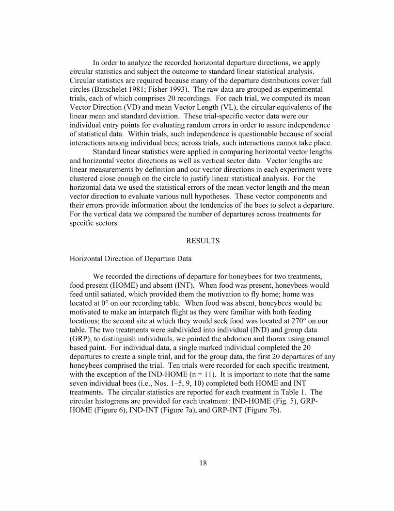
We recorded the directions of departure for honeybees for two treatments, food present (HOME) and absent (INT). When food was present, honeybees would feed until satiated, which provided them the motivation to fly home; home was located at 0° on our recording table. When food was absent, honeybees would be motivated to make an interpatch flight as they were familiar with both feeding locations; the second site at which they would seek food was located at 270° on our table. The two treatments were subdivided into individual (IND) and group data (GRP); to distinguish individuals, we painted the abdomen and thorax using enamel based paint. For individual data, a single marked individual completed the 20 departures to create a single trial, and for the group data, the first 20 departures of any honeybees comprised the trial. Ten trials were recorded for each specific treatment, with the exception of the IND-HOME (n = 11). It is important to note that the same seven individual bees (i.e., Nos. 1–5, 9, 10) completed both HOME and INT treatments. The circular statistics are reported for each treatment in Table 1. The circular histograms are provided for each treatment: IND-HOME (Fig. 5), GRP-HOME (Figure 6), IND-INT (Figure 7a), and GRP-INT (Figure 7b).

18

Table 1 – Circular statistics of the 4 different treatments (Trial and Lumped Data), with n being the number of trials or bees.

Treatment Trial Data Lumped Data

Mean VD Mean VL n Mean VD Mean VL N

IND-HOME 2.05 ± 4.30° 0.770 ± 0.05 11 1.20° .750 220

GRP-HOME 12.88 ± 3.70° 0.750 ± 0.03 10 12.50° .737 200

IND-INT 266.87 ± 4.59° 0.730 ± 0.04 10 266.47° .709 200

GRP-INT 259.01 ± 4.74° 0.729 ± 0.05 10 259.42° .709 200

Figure 5 – 20 homeward departures for 11 individual bees. The dot represents the direction home.

19

Figure 6 – 10 trials of homeward departures of group data. Each trial consists of 20 departures. The dot represents the direction home.

20

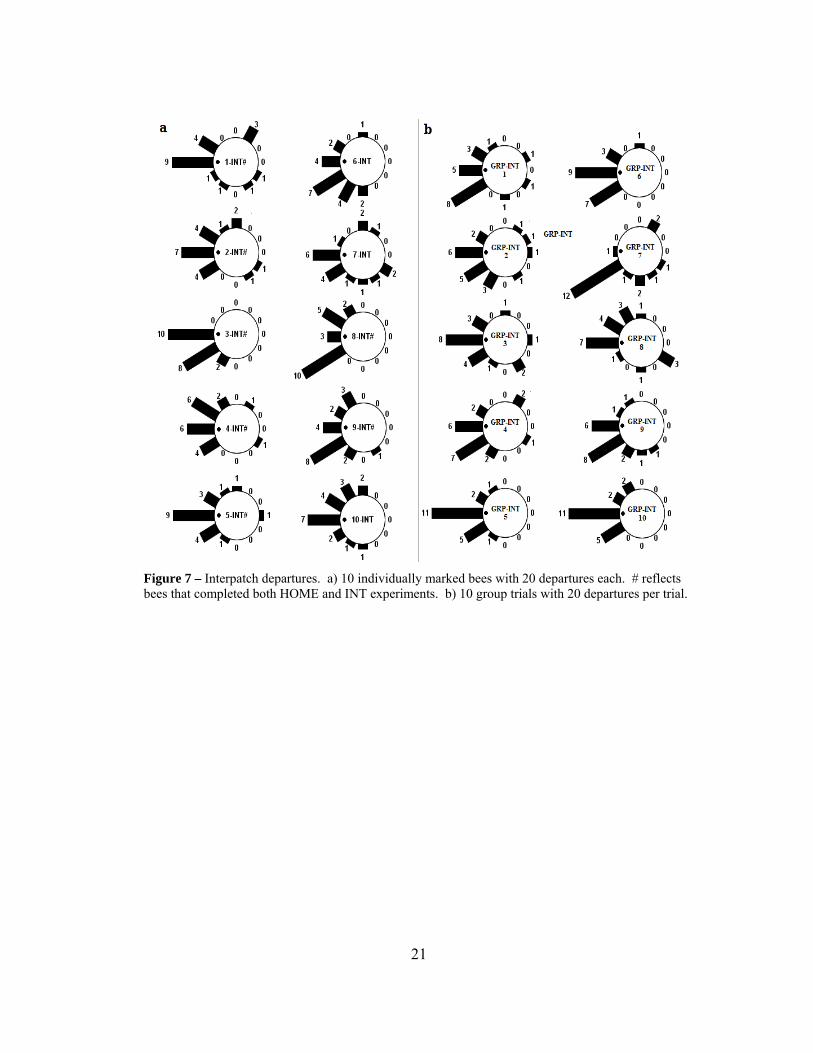
Figure 7 – Interpatch departures. a) 10 individually marked bees with 20 departures each. # reflects bees that completed both HOME and INT experiments. b) 10 group trials with 20 departures per trial.

21

Figure 8 – Lumped histograms for the 4 different treatments. There is no statistical difference between the departure direction of similar conditions (a and b, c and d; p>.05). There are extreme statistical differences between the directional departure of dissimilar conditions (a and c, a and d, b and c, b and d; p<.00001)

Lumped Data

We summed the sectors of all histograms for each of the four treatments to obtain lumped histograms, used to assess the overall distribution (Fig. 8). The statistics for the lumped data are also in Table 1.

Statistical Tests

Two null hypotheses were formulated for the mean vector directions (VD) and tested using standard linear t-tests. To validate the utility of recording initial departures (e.g., 50 cm from the feeder), we compared the observed mean VD to the expected VD (the actual direction on the table) with a one-sample t-test and found no significant difference among all treatments, p > 0.05. We also compared the observed mean VD of individually marked bees to the observed mean VD of groups of bees (not individually marked) with a two-sample t-test (Table 2). When the expected mean VD was the same between our treatments (IND-HOME vs. GRP-HOME; IND-INT vs. GRP-INT) we found no significant difference, p > 0.05. When the expected mean VD was different between treatments (IND-HOME vs. IND-INT; IND-HOME vs. GRP-INT; IND-INT vs. GRP-HOME; GRP-HOME vs. GRP-INT) there was an extreme difference, p < 0.00001. We conclude that the bees, in all cases, knew the direction to home and to the other feeding site. We also conclude that they have the ability to choose between both depending upon their motivational state.

22

We then compared the mean vector lengths (VL) amongst trials using two-sample t-tests (Table 3). We found that, regardless of our treatment, the mean VL was never different between any of the tests (p > 0.05), with a grand mean of 0.745. Table 2 – The results of the two-sample t-tests for equal vector directions (VD). Individual departures are not different than the group departures, using this method.

Vector Direction Test t p df

IND-HOME vs. GRP-HOME 1.918 0.07035 18.84

IND-INT vs. GRP-INT 1.191 0.24922 17.98

IND-HOME vs. IND-INT 15.194 <0.00001 18.70

IND-HOME vs. GRP-INT 16.157 <0.00001 18.53

IND-INT vs. GRP-HOME 17.993 <0.00001 17.21

GRP-HOME vs. GRP-INT 18.940 <0.00001 16.98

Table 3 – The results of the two-sample t-tests for equal vector lengths (VL). All treatments show equal departure tendency, regardless of the direction.

Vector Length Test t p df

IND-HOME vs. GRP-HOME 0.367 0.717 18.71

IND-INT vs. GRP-INT 0.011 0.991 17.95

IND-HOME vs. IND-INT 0.672 0.509 18.85

IND-HOME vs. GRP-INT 0.665 0.513 18.64

IND-INT vs. GRP-HOME 0.367 0.717 17.24

GRP-HOME vs. GRP-INT 0.368 0.717 16.87

Quality Control – The removal of systematic errors

In presenting a new method, we have to account for any systematic errors inherent in our design. Because we stand near the data collection table during testing,

23

we create a large obstruction on one side of the table that may bias the honeybees' direction of departure. To account for this bias, half the data per trial are taken with the observer on one side of the table and the other half with the observer on the opposite side of the table. We then tested this effect by analyzing the departures when standing on either side of the table. We conclude that the two distributions are not statistically different (p > 0.05) and that our positioning does not significantly alter directional departure decision making. The resulting lumped histograms are shown in Figure 9a. When we observe the behavior of departing bees, we use objective criteria to specify what we can call a true departure. We do this for two reasons. First, the certainty of motivational state is necessary; if they depart based upon motivations other than hunger or satiation, they are not relevant to our investigation. Second, this reduces the noise in the data as we must not select non-departures, allowing us a better means to observe the decision making of motivated and familiarized bees. To analyze the effect of our objective criteria we video recorded a typical interpatch test. During video analysis we called departures using the objective criteria and then without any departure criteria whatsoever. For the latter, we watched the video 12 separate times (one for each sector) and counted any bee that flew past the margin of the table. We conclude that the mean vector direction is not statistically different (p > 0.05), indicating our familiarity training provides adequate directional departure decision making, independent of our objective criteria. We also conclude that there is a difference in the mean vector length when we use our objective criteria and without (VL = 0.624 and 0.373, respectively); when our objective criteria are applied the mean vector length is higher. This data indicates that our objective criteria are sufficient in reducing the influence of departures made under irrelevant motivations as well as eliminating non-departures. These resulting lumped histograms are shown in Figure 9b.

24

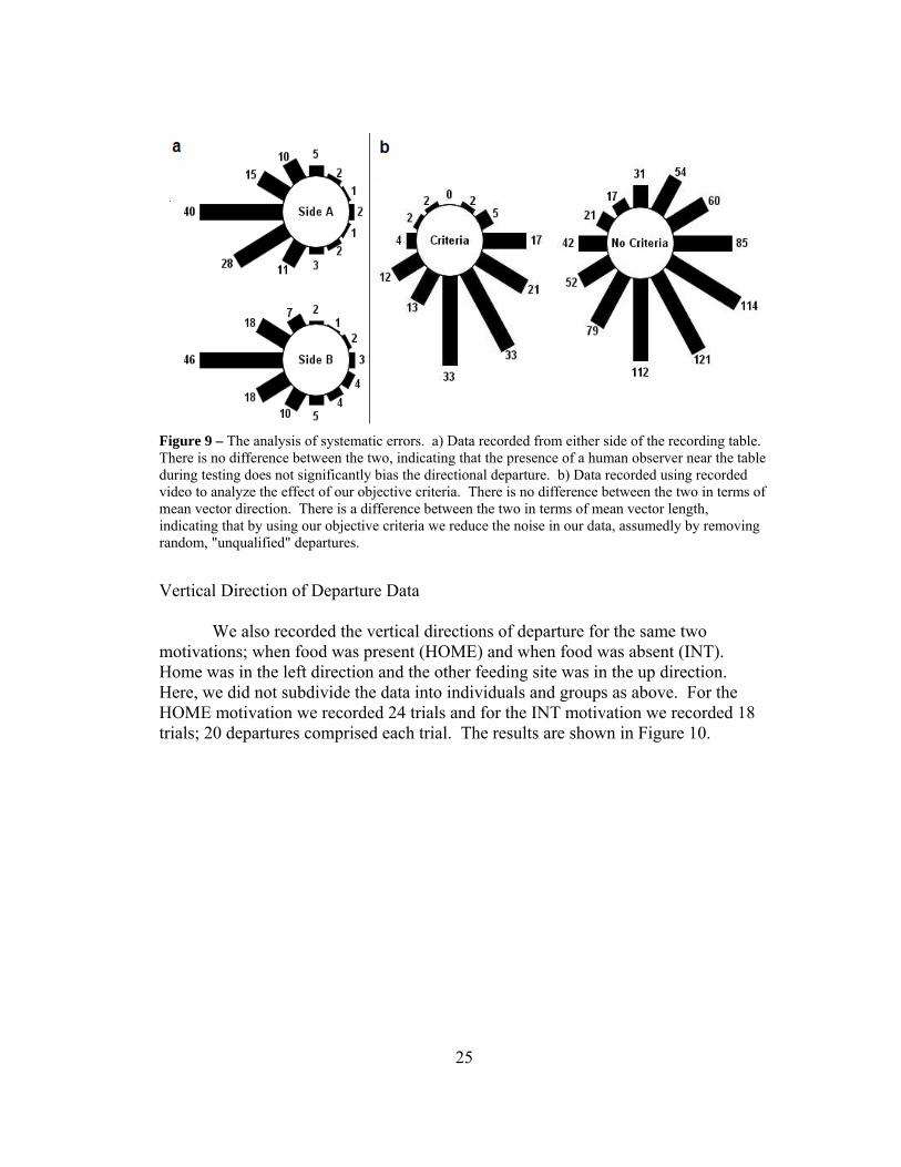
Figure 9 – The analysis of systematic errors. a) Data recorded from either side of the recording table. There is no difference between the two, indicating that the presence of a human observer near the table during testing does not significantly bias the directional departure. b) Data recorded using recorded video to analyze the effect of our objective criteria. There is no difference between the two in terms of mean vector direction. There is a difference between the two in terms of mean vector length, indicating that by using our objective criteria we reduce the noise in our data, assumedly by removing random, "unqualified" departures.

Vertical Direction of Departure Data We also recorded the vertical directions of departure for the same two motivations; when food was present (HOME) and when food was absent (INT). Home was in the left direction and the other feeding site was in the up direction. Here, we did not subdivide the data into individuals and groups as above. For the HOME motivation we recorded 24 trials and for the INT motivation we recorded 18 trials; 20 departures comprised each trial. The results are shown in Figure 10.

25

Figure 10 – Data from vertical departures under home and interpatch motivations. Left is the direction of home and up is the direction of the interpatch path. The error bars represent standard deviation.

Statistical Tests

Two null hypotheses were formulated for the counts in the three categories. We compared the amount of departures through the left sector between our two treatments (HOME vs. INT) with a two sample t-test and found a significant difference (p < 0.001) with the HOME motivation having more departures. Next we compared the up sector between our two treatments with a two sample t-test and found a significant difference between the two (p < 0.001) with the INT motivation having more departures. We conclude that these bees also knew the direction to home and to the other feeding site, being able to choose between both depending upon their motivational state. Here, the third dimension appeared to pose no problem.

DISCUSSION Theoretical Importance These new experimental methods will provide novel information about the complexity of honeybee foraging for three reasons. First, they allow the analysis of interpatch foraging, which has lacked adequate study in comparison to hive based foraging (outward and homeward paths). Attempting to describe this foraging knowledge using only two out of at least three fundamental foraging paths is likely to lead to inaccurate descriptions, especially when those two paths are intimately associated with communicated information (waggle dances) as well as individual

26

experience. The interpatch path is the best way to separate these two sources of information and investigate only the individual experience or primary learning. Second, training honeybees to be familiar with an interpatch foraging regimen has highly significant benefits. Specifically, we can define the sources of information available to the honeybee as it makes its immediate decision (flight path of 0.5 m) with unprecedented accuracy, giving us a superior advantage in the analysis of decision making. We can also more easily control the motivational state by simple alternation of food availability. Previous attempts to analyze decision making have been dependent on so called "vanishing bearing" departure data. This procedure involves observers visually tracking a bee as long as possible and recording the compass bearing of the location at which the bee "vanished" from sight; there are some fundamental disadvantages with this procedure. For instance, the duration of tracking leaves plenty of room for the bees to use updated information (not present at the exact point of release or departure); this extra information is impossible to control for. Another disadvantage is that the bees are quite capable of making more than one decision during the tracking time such that the direction they are flying may not correlate with the direction of the compass bearing the observer records; this causes a misrepresentation of the decision making. Lastly, the distance at which bees “vanish” from sight is inconsistent for a variety of reasons; visual resolution and tracking ability varies tremendously among individuals. Our method has none of these disadvantages. Third, our honeybees are allowed to forage under more natural conditions as they are provided ample time to become familiar with the surroundings and are allowed to use and learn all cues. Given such circumstances, we can remove the need for physical displacement. Instead, we can experimentally assign certain cues with utility, while others have none. Our ability to specifically define all sources of information gives us extraordinary power. We can add, remove, or combine information to discover exactly what bees are capable of learning, ignoring, and linking together. If needed, however, this method can fully handle displacements. Presented Interpatch Data With the data presented here, we are able to answer two of the questions asked in the introduction. Do honeybees remember and recognize the locations of multiple food patches they visit on a single trip? This memory is the fundamental principle behind interpatch foraging. Not only did the honeybees know the two foraging locations, but they linked them together cognitively based upon food availability. This understanding can be represented as a simple contingency; if no food is present, then go to other associated location. The ecological relevance is that sometimes food will not be available where the honeybee expects it and instead of going home it goes to another place of expectation. At this point, it is irrelevant as to how the bees make this decision or what cues are used to guide their departures; this method can easily solve these open questions.

27

An additional intriguing observation is that initially, it makes sense for honeybees to know how to get from one feeder to the other because they were incrementally trained to learn the path. However, our observations have revealed that if you paint honeybees after such training, they will eventually be replaced by young bees as they die off. The new individuals that continue to show up are not painted and seem to understand equally well, but without the incremental training. Understanding how they are capable of learning this association is intriguing and can easily be discovered with this method, but was not our focus here.

Do honeybees know what routes to fly in three-dimensional space when flying from food source to food source? Given the results in Figure 10, we can safely say that these honeybees can handle this problem. This ability is expected as honeybees have been shown to understanding of the third dimension when flying to a food site from the hive (Von Frisch 1967). It also adds a new understanding of how rich their understanding of the world is away from the colony. Group Data We found no significant difference between our individually marked honeybees and the corresponding group data (Table 2). This result is functionally important. Data from individually marked honeybees have become a standard for foraging experiments; such data are easy to obtain if the honeybees are individually captured and displaced. Because our experimental design does not require captures or displacements, the honeybees learn and forage under more natural conditions. Our experimental tests involve removal of food from all sites, and then observing the departure of the bees. The longer food is absent from all sites, the more likely the training of the bees is disrupted.

The use of individually marked bees requires a longer time during experimental tests because you must rely on them to arrive at the testing feeder and satisfy all departure criteria. To put this into perspective, the data for the individual bees presented in figure 7a were gathered in about six hours. In contrast, the group data presented in figure 7b required less than 20 minutes to gather. After calculation, individual data takes roughly 18 times longer to obtain the same information; the data presented here is also without extra experimental manipulations, making it relatively easy data to obtain. The time required for testing during experimental manipulations must be minimized to prevent loss of learning (there is no food or reward during testing). We can obtain a group trial of 20 honeybees in less than 1 min, but we would not expect more than a single departure from two individually marked honeybees in the same time, satisfying the departure criteria. Group data allows us to make the same conclusions as using individually marked bees and is a better tool given our design. If needed, however, individual data can still be obtained, yet we argue that it is more important to uncover the general skill set first, and then probe for the inter-individual differences. Use of group data has statistical consequences. Because honeybees are social and interact, each individual honeybee departure may not be independent. Trial data

28

must be used instead of data on single honeybees as such social interactions cannot occur between trials. However, the statistical measures for trial data (n = 10 trials) and for lumped data (n = 200 bees) are the same (VD - Table 1, VL – not shown); we make the same conclusions from the data, regardless if it is trial or lumped data. To maintain statistical responsibility however, we conservatively rely on trial data. Even with this conservative group data, our ability to detect differences between treatment groups is powerful (Table 2). The honeybees make their departure directions spatially distinct. Correspondingly, we found no differences between vector lengths (Table 3). This data indicates that the honeybees are equally motivated to depart toward home when satiated or towards the other location when hungry. Harmonic Radar

Harmonic radar is another new and recent investigatory tool that has been used to chart the entire flight paths of honeybees at short distances from the hive (Riley 1996). Without a doubt, there is great power in this tool for discovering some fundamental principles about honeybee biology—paramount was the final proof of the dance communication (Riley et al 2005). In the context of interpatch foraging, however, this method has little advantage over our proposed methods. The initial decision making of a honeybee is much easier viewed from 0.5 m than the poor resolution of radar tracking and the location of the decision is exactly the same for every bee. Also, as the distance between our feeding sites is often less than 20 m, the full interpatch flight path can be visually tracked or recorded by video.

The great disadvantages of harmonic radar are sample size, line of sight, radar maintenance, and cost of operation. Our method has none of these disadvantages and provides higher quality information with respect to decision making. We can put a table in any square meter area: in dense trees, on all sides of a building, above and below slopes, and even in unfavorable weather. Place Recognition

Snapshot Theory

Current place recognition theory stipulates that honeybees seek to match visual stimuli patterns to stored retinal images or snapshots of the locality (Cartwright and Collett 1983). These snapshots then allow departure direction decisions. During our testing periods, where an observer stands next to the recording table, the local arrangement of objects and visual field of the bees is changed drastically. To match such a 'testing period' stimuli pattern (including the observer) to a stored snapshot (lacking the observer) is likely not a straightforward procedure. In fact, the honeybees appear to have the ability to ignore us completely (Fig. 9a) as long as we are not standing in exactly the same place every time. This result implies that in their place recognition machinery, there is an ability to ignore objects that are not reliable landmarks, or are constantly changing location. Thus, the term 'snapshot' is

29

misleading as a true snapshot could not correct for such obstruction and randomly appearing or disappearing objects—the place recognition machinery of the honeybee is more complicated.

Expectation and Place Characterization When a foraging honeybee leaves the hive, they have an expectation of reality. This expectation applies to honeybees that follow dances as well as for the scout bees in the morning that show up before food. They know about the location of places and the characteristics of those places (odor, color, temporal availability, etc.). Given our current knowledge, we do not know how dynamic their expectations can be and have lacked the adequate means to investigate them. The ability to precisely control the information used in decision making, provided by our new method, will allow us to discover how much honeybees know about the land around them and the ecology of the resources they are dependent on, primarily flowering plants. Route Planning and Cognitive Information It seems the honeybee, an extremely capable invertebrate, is always under one controversy or another. The most distinguished controversy of the past (Gould 1976, Munz 2005), debated whether the honeybee dances guided recruits to food or odor cues did. In those times, each side was well defined as there were distinct options. In our current controversy, it is clearly not as distinguished. Most unfortunately, the current descriptions of the cognitive skills come in essentially two forms: the lack of a cognitive map and the presence of it. Here, there are well defined concepts such as landmark orientation and serial route knowledge in the lack of cognitive map category. However, under the category of cognitive map, there is no consistent definition to the point that “verifying it” is almost useless; our justifications lack a consistent framework. Even some of the most interesting data in the context of “cognitive mapping” only refers to the honeybees’ capabilities as “map-like”, forcing important information into the dichotomous controversy reprising the elusive concept (Menzel et al. 2005).

Somewhere within the confusion, there have been some fundamental questions in terms of how honeybees plan their routes. Specifically, what cues are used for recall and how is the information stored in long term memory? Our method will provide clearer answers to the questions already asked as well as introduce new questions that, until now, were incapable of being tested. Simultaneously, the use of our new place map concept will relieve the constraints of doing experiments to validate a confused ‘cognitive map’ concept and allow the description of the complex additions to the basic place map. We anticipate many complex additions within the honeybee as well as a gradient of place maps among many diverse species, differing qualitatively and quantitatively depending on their ecological constraints and necessities. Once these fundamental aspects of cognition are revealed, the more puzzling questions will emerge. How much information can the nervous system

30

handle and which sensory modalities take priority and under which contexts? Our method can easily handle these questions. The Mind of a Bee Colony

When we think of honeybees, their success is phenomenal and is always measured by the performance of the colony (Seeley 1996), not an individual. The colony relies on the waggle dance and the great majority of the honeybees are capable of interpatch foraging. These are two independent ways we, as scientists, are able to investigate their knowledge. Our progression of investigations must be efficient. We aim to uncover the detailed capabilities of the colony, but our method is flexible enough to handle individual knowledge as well. It is time to divorce ourselves from the dance language, or any foraging paths linked to the dance, as needed. We need a new window to peek into the mind of one of the most efficient foragers in existence. And here, we present the methods to analyze this most important foraging path, the interpatch path, to discover how good these honeybees are.

31

Chapter 2

Investigating Landmark Theory Background Landmark theory, no matter how complex the details were, implies the use of terrestrial cues. Subsequently, honeybees would need to use terrestrial cues in order to fly interpatch paths consisting of both distance and direction components; we started by investigating direction.

Within terrestrial cues there are many things that can guide you to your goal. The most direct is the beacon, a conspicuous object that is directly associated with the goal itself. For example, a beacon could be a large tree with the resource nearby. As the tree is easier to localize from great distance, it becomes a beacon that is directly approached. Unfortunately, not all food sources come with conspicuous beacons and other things must be used.

Terrestrial compass cues involve knowing the direction based upon cues not directly associated with the goal. Instead, the goal can be in the same direction as some distal compass cue like a mountain. Also, if a honeybee is flying in a square grassy area surrounded by trees (easy to find in modern cities) it might use the tree edge to know that the goal is in one specific corner of the tree edge. Here the geometric layout of the terrestrial cues provides a direction that is indirectly related to the goal.

It must also be mentioned that celestial cues can be used as a compass as well (Dyer and Gould 1981). Our method allows us to test them simultaneously or one at a time. We wanted to look at these various possibilities and test them one by one. Our first test then, described in the experiment below, specifically separates beacon from compass knowledge, but did not differentiate between terrestrial or celestial compass knowledge.

Problems with Previous Experiments

Without a doubt, there are many types of terrestrial cues, but they all fall into these categories, beacons and terrestrial compass cues. Lucky for us, these are almost mutually exclusive and given smart experimental planning, can be made to be so.

The first problem was that these navigational strategies were debated as either/or by investigators. We argue that the specific answers each researcher found were dependent upon experimental context far more than navigational capability. Our data (given from the experiment below) shows that given the exact same context, honeybees have the ability to choose between both.

The second problem was that none of the previous experiments were able to say exactly what sources of information the honeybees were using. One major reason for this inability was due to the use of vanishing bearings. In the experiment from chapter 1 we talk about the inefficiencies of such vanishing bearings. The other

32

major reason for this inaiblity is due to displacement of honeybees. We do not accurately know either the motivational states these honeybees were in or what cues they used when they choose a particular direction. The following experiment successfully removes both of these errors. Our immediate decisions unify and equalize all sources of information to a single point while our interpatch familiarity allows us to exactly separate the sources of information used for navigational decision making.

The last problem was that many of these experiments came from experiments not involving interpatch paths. We remedy this by using only interpatch paths.

The experiment below is our first investigation of landmark theory. This experiment can be set up, trained, and finished over a weekend. Consequently, this experiment can be toned down and made into a laboratory experiment for behavior labs.

33

The Interpatch Path – How Honeybees Choose a Direction

Danny Najera, Patty Van Meter, Rudolf Jander

INTRODUCTION

When a honeybee flies between two resource locations (interpatch foraging) it must use some way finding mechanism; two general mechanisms are beacon orientation and compass navigation. Beacon orientation can be defined as direct approach to a conspicuous stimulus at or near the goal location. Compass navigation can be defined as the use of stimuli not directly associated with the goal in order to direct the heading; compass cues can be either terrestrial or celestial for honeybees, or both (Von Frisch and Lindauer 1954, Capaldi and Dyer 1995). Knowledge about the relative role of compass navigation and beacon orientation has been of great interest in the context of topographic cognitive mapping. Gould (1986) argued that bees can use map-based compass navigation to move between foraging patches, whereas Dyer (1991) and Cheng (2000) emphasize the possibility of beacon orientation as an alternative explanation for this particular spatial task. In no case were these potential mechanisms completely isolated or compared, and in many cases were confounded by potential communicated knowledge from dances; a honeybee flying an interpatch path utilizes information only from its own past experience, permitting us easier separation of these different mechanisms. Using our new experimental technique (self reference - Chapter 1) we present the first investigation on the relative role beacon orientation and compass navigation have on directional decision making, in the context of interpatch foraging.

GENERAL METHODS

Experimental Design

Training

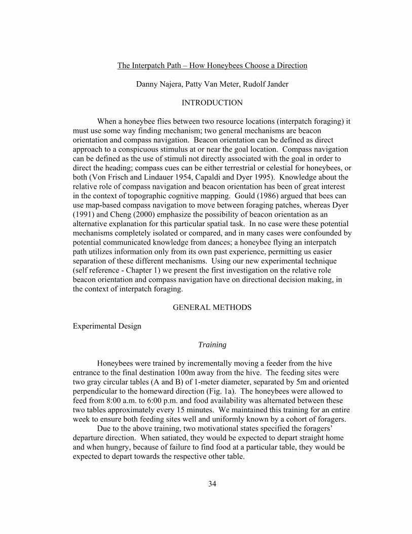
Honeybees were trained by incrementally moving a feeder from the hive entrance to the final destination 100m away from the hive. The feeding sites were two gray circular tables (A and B) of 1-meter diameter, separated by 5m and oriented perpendicular to the homeward direction (Fig. 1a). The honeybees were allowed to feed from 8:00 a.m. to 6:00 p.m. and food availability was alternated between these two tables approximately every 15 minutes. We maintained this training for an entire week to ensure both feeding sites well and uniformly known by a cohort of foragers. Due to the above training, two motivational states specified the foragers’ departure direction. When satiated, they would be expected to depart straight home and when hungry, because of failure to find food at a particular table, they would be expected to depart towards the respective other table.

34

Data Collection

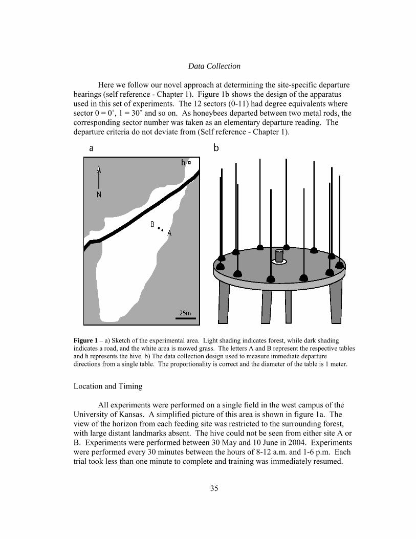
Here we follow our novel approach at determining the site-specific departure bearings (self reference - Chapter 1). Figure 1b shows the design of the apparatus used in this set of experiments. The 12 sectors (0-11) had degree equivalents where sector 0 = 0˚, 1 = 30˚ and so on. As honeybees departed between two metal rods, the corresponding sector number was taken as an elementary departure reading. The departure criteria do not deviate from (Self reference - Chapter 1).

Figure 1 – a) Sketch of the experimental area. Light shading indicates forest, while dark shading indicates a road, and the white area is mowed grass. The letters A and B represent the respective tables and h represents the hive. b) The data collection design used to measure immediate departure directions from a single table. The proportionality is correct and the diameter of the table is 1 meter.

Location and Timing All experiments were performed on a single field in the west campus of the University of Kansas. A simplified picture of this area is shown in figure 1a. The view of the horizon from each feeding site was restricted to the surrounding forest, with large distant landmarks absent. The hive could not be seen from either site A or B. Experiments were performed between 30 May and 10 June in 2004. Experiments were performed every 30 minutes between the hours of 8-12 a.m. and 1-6 p.m. Each trial took less than one minute to complete and training was immediately resumed.

35

Statistical Analysis Our procedure did not deviate from (self ref – chapter 1). In this set of expeimrents, our trial data included 30 departures per trial (15 on each side of the recording table), providing the vector direction (VD) and vector length (VL), the circular equivalents of the mean and standard deviation. In some experiments the departing bees preferred two, instead of one, departure direction. Two different statistical procedures of rejecting unimodality versus bi-modality will be explained below together with the respective data. It was also useful to look at the data as quadrants, which in our design, consisted of the Home (sectors 11,0,1), East (2,3,4), South (5,6,7), and West quadrants (8,9,10).

EXPERIMENT 1 – CONTROL DEPARTURES

Methods We first tested honeybees that were motivated to return home (Home), recording the departures of satiated bees. For both tables, sector 0 would represent the direction to home. We then tested honeybees that were motivated to fly to the other feeding site for food (Food), recording the departures of hungry bees that did not discover food where they first expected it. For table A, the sector 9 would represent the direction to table B. For table B, the sector 3 would represent the direction to table A. Results (Fig. 2) Fully satiated foragers on tables A and B departed in the homeward (around 0˚) direction. As the expected home directions for tables was the same (sector 0), the data was lumped together; “HomeAB” represents the departures from both tables under the Home-motivation. The Home quadrant comprised 73.3% of all departure bearings. Hungry foragers that failed to find food after arriving at table A departed towards table B (around 270˚) with the West quadrant comprising 68.3% of all departure bearings. Finally hungry foragers that failed to find food after arriving at table B departed toward table A (around 90˚), with the East quadrant comprising 69.1% of all departure bearings. Departures from table A were designated “FoodA” and those from table B, “FoodB”.

36

Figure 2 – Immediate departure directions from Experiment 1. Numbers inside the circle represent sectors, while numbers outside the bars represent the bee departures through the respective sector. HomeAB represents departures of satiated bees, where 0 is the direction home; tables A and B were lumped together. FoodB represents departures of hungry foragers departing from table B where sector 3 (90º) is the direction to table A. FoodA represents departures of hungry foragers departing from table A where sector 9 (270º) is the direction to table B. VD and VL are the mean vector directions and lengths with their standard errors and n is the number of trials underlying each histogram.

EXPERIMENT 2 – BEACON VS. COMPASS ORIENTATION Methods From experiment 1, when our hungry foragers departed in the direction of the respective other feeding table, beacon or compass cues may have been utilized. To distinguish between them, we experimentally separated the two cues by displacing the respective goal tables, the potential beacons, along an arc of either 180˚ (Exp. 2-180) or 90˚ (Exp. 2-90), while maintaining the 5 meter inter-table distance. This displacement occurred immediately before a trial and took less than 3 seconds to perform. For the 180˚ movements, 11 trials per table were performed and for the 90˚ movements, 7 trials per table were performed. Statistics – 180˚Arc In this experiment, the histograms of the departure bearings are visually bimodal (Fig. 3). Hence, instead of the mean departure vector we have to compute the mean axis vector direction (VAD) and the mean axis vector length (VAL) that are

37

defined by the following computational procedure; this would allow us to statistically validate the bimodality. A test of bimodality (180˚ difference in modes) for circular data is commonly called “doubling the angles” (Batschelet 1981). For example, a hypothetical situation of directions 0˚, 90˚, 180˚, and 270˚ would transform into 0˚, 180˚, 360˚, and 540˚. As circular data repeats indefinitely, 0˚ and 360˚ become equivalent, as do 180˚ and 540˚, with the data of both initial directions summed together in a new direction. The new distribution then consists of 6 sectors (0-5) with twice the original statistical weight. If the mean vector length of the new distribution (VAL) is significantly greater than the original, this is taken as evidence for a bimodal distribution. For our particular situation, the bimodality existed primarily between sectors 3 and 9 for both tables (90˚ and 270˚), and after doubling the angles, sectors 3 and 9 would line up as sector 3 (180˚ and 540˚). Results – Exp. 2 – 180˚Arc (Fig. 3) The computed statistical values and their errors are compatible with the assumption of bimodality (Fig. 3). The summed percentages of departures in the East and West quadrants were 78.5% for table A and 79.6% for table B. These percentages are somewhat higher than those in the unimodal distributions of Experiment 1.

38

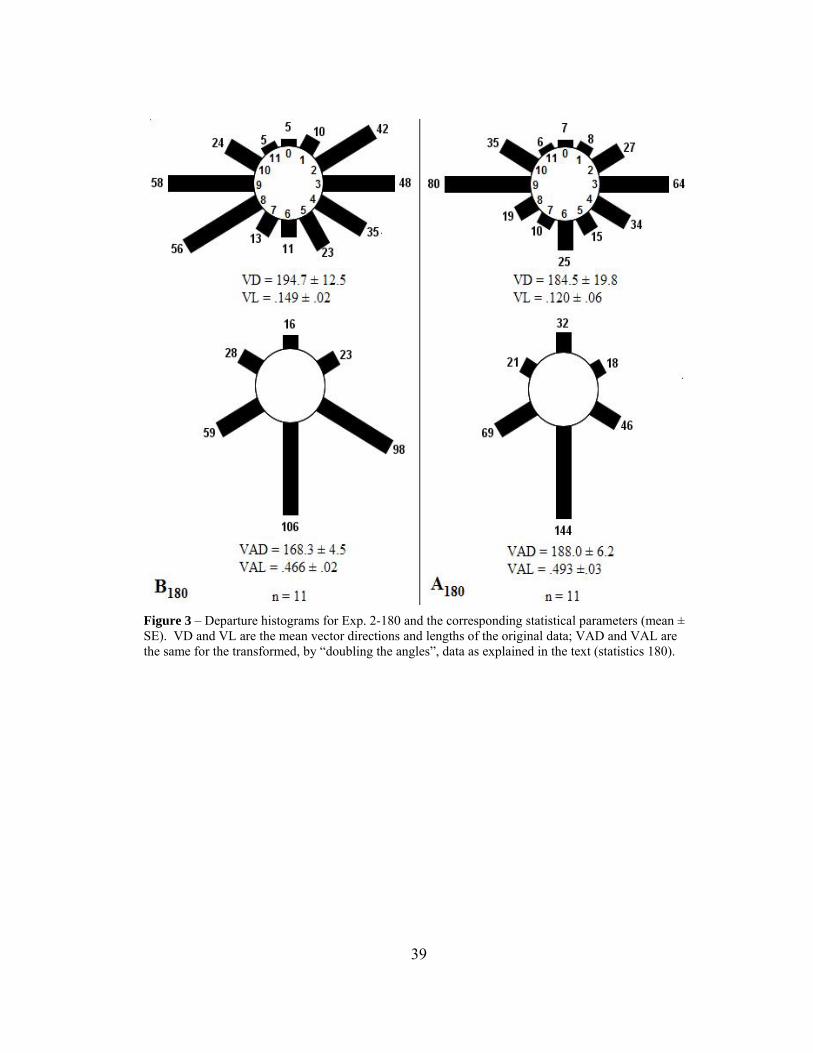
Figure 3 – Departure histograms for Exp. 2-180 and the corresponding statistical parameters (mean ± SE). VD and VL are the mean vector directions and lengths of the original data; VAD and VAL are the same for the transformed, by “doubling the angles”, data as explained in the text (statistics 180).

39

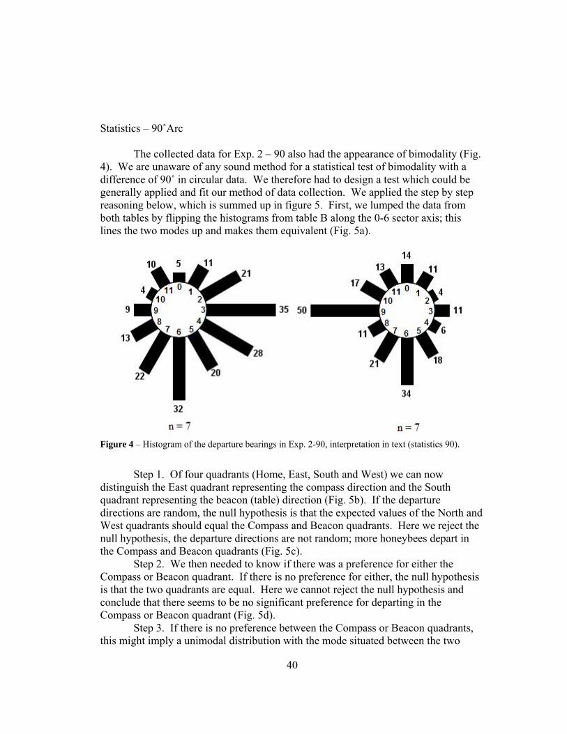
Statistics – 90˚Arc The collected data for Exp. 2 – 90 also had the appearance of bimodality (Fig. 4). We are unaware of any sound method for a statistical test of bimodality with a difference of 90˚ in circular data. We therefore had to design a test which could be generally applied and fit our method of data collection. We applied the step by step reasoning below, which is summed up in figure 5. First, we lumped the data from both tables by flipping the histograms from table B along the 0-6 sector axis; this lines the two modes up and makes them equivalent (Fig. 5a).

Figure 4 – Histogram of the departure bearings in Exp. 2-90, interpretation in text (statistics 90).

Step 1. Of four quadrants (Home, East, South and West) we can now

distinguish the East quadrant representing the compass direction and the South quadrant representing the beacon (table) direction (Fig. 5b). If the departure directions are random, the null hypothesis is that the expected values of the North and West quadrants should equal the Compass and Beacon quadrants. Here we reject the null hypothesis, the departure directions are not random; more honeybees depart in the Compass and Beacon quadrants (Fig. 5c). Step 2. We then needed to know if there was a preference for either the Compass or Beacon quadrant. If there is no preference for either, the null hypothesis is that the two quadrants are equal. Here we cannot reject the null hypothesis and conclude that there seems to be no significant preference for departing in the Compass or Beacon quadrant (Fig. 5d). Step 3. If there is no preference between the Compass or Beacon quadrants, this might imply a unimodal distribution with the mode situated between the two

40

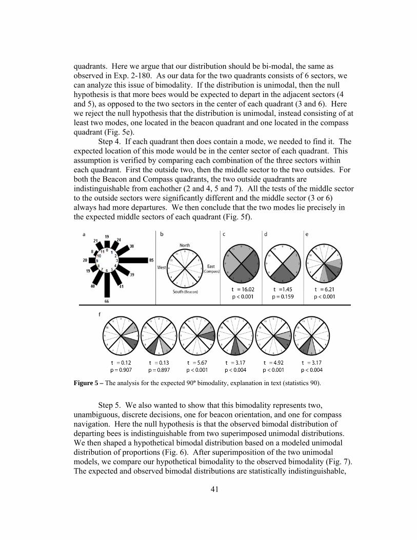
quadrants. Here we argue that our distribution should be bi-modal, the same as observed in Exp. 2-180. As our data for the two quadrants consists of 6 sectors, we can analyze this issue of bimodality. If the distribution is unimodal, then the null hypothesis is that more bees would be expected to depart in the adjacent sectors (4 and 5), as opposed to the two sectors in the center of each quadrant (3 and 6). Here we reject the null hypothesis that the distribution is unimodal, instead consisting of at least two modes, one located in the beacon quadrant and one located in the compass quadrant (Fig. 5e). Step 4. If each quadrant then does contain a mode, we needed to find it. The expected location of this mode would be in the center sector of each quadrant. This assumption is verified by comparing each combination of the three sectors within each quadrant. First the outside two, then the middle sector to the two outsides. For both the Beacon and Compass quadrants, the two outside quadrants are indistinguishable from eachother (2 and 4, 5 and 7). All the tests of the middle sector to the outside sectors were significantly different and the middle sector (3 or 6) always had more departures. We then conclude that the two modes lie precisely in the expected middle sectors of each quadrant (Fig. 5f).

Figure 5 – The analysis for the expected 90º bimodality, explanation in text (statistics 90).

Step 5. We also wanted to show that this bimodality represents two, unambiguous, discrete decisions, one for beacon orientation, and one for compass navigation. Here the null hypothesis is that the observed bimodal distribution of departing bees is indistinguishable from two superimposed unimodal distributions. We then shaped a hypothetical bimodal distribution based on a modeled unimodal distribution of proportions (Fig. 6). After superimposition of the two unimodal models, we compare our hypothetical bimodality to the observed bimodality (Fig. 7). The expected and observed bimodal distributions are statistically indistinguishable,

41

within the margin of error (with the exception of sector 1, which we believe to be non-informative in this context). We then conclude that the honeybees unambiguously decide to depart either in the compass or the beacon direction, but do not choose intermediately. To cement or statistical argument of bimodality (for 90º) we also looked at an independent measure of the bimodality. Here, we took the original data (Fig. 4) and ranked the sectors according to the amount of departures recorded in them. The two sectors which had the highest departures were assigned degree equivalents and the difference was then calculated. When two sectors tied for the 2 highest departures, the difference was simply calculated between them. When the sector with the most departures was defined, but the next highest had ties from 2 or more sectors, we averaged the tied sectors and used that average to calculate the difference; one outlier trial was thrown out when the difference came to 0. This procedure was completed for both the superimposed model (one had to be thrown out as an averaged quantity canceled out the original direction) and the original data. For the superimposed model, the average difference, was 80.9 ± 3.4º (mean + SE, n = 49), and for the original data, 81.0 ± 7.4º (n = 14); there was no statistical difference between these two (t18 = .02, p = .988).

Figure 6 – Modeled unimodal distribution of directional proportions. Modeling included 50 separate trials, all of which were performed under the hungry motivation, but vary in the time of day, time of year, different years, and amount of departures per trial.

42

Figure 7 – The comparison of the hypothetical bimodality, composed of two identical unimodal models superimposed on top of each other. No statistical difference was observed between sectors of the model and the experimental data with the exception of sector 1, which we believe to be non-informative. Results Exp. 2 - 90˚Arc (Fig 4) After the respective movement of the destination table 90 degrees, the honeybees again departed preferentially in two directions, one in the original compass direction (sectors 9 and 3, for tables A and B respectively) and the other towards the displaced beacon (sector 6 for both tables) (Fig. 4). Looking at the original data for A90, the perpendicular sectors 6 and 9 received the highest amount of individual departures. Also the sum of departures through the West and South quadrants represent 71.9% of the data. For B90, the perpendicular sectors 6 and 3 received the highest amount of individual departures, while the sum of departures through the East and South quadrants represented 75.2% of the data.

DISCUSSION

Decision Making Satiated honeybees are motivated to go home, decide to go home, and immediately depart in the direction of home. Honeybees not finding food where they expect it are motivated to fly to the other feeding site, decide to, and immediately depart in the direction of the other feeding site. As mentioned in (Self Ref - Chapter 1) this type of decision making is wholly dependent on our familiarization training, which allows us the following advantage. Because the immediate decisions are being made based on information, and because all the information is present at the position of the table, we are able to define the sources of information used in decision making more clearly than ever before. Previous "vanishing bearing" departure data leaves

43

plenty of room for the bees to use updated information and more than one decision. This information, which a honeybee uses for its single, immediate departure, can consist of beacon information and compass information; this led to experiment 2. Beacon Orientation and Compass Navigation Separation The first conclusion we can make is that the table was acting as a beacon, thus allowing the bees to directly approach a conspicuous object associated with the goal; this beacon then determined their departure direction. We know this because given the results of experiment 1 – FoodA, there were no significant number of departures through the East quadrant or the South quadrant. The same is true for the West and South quadrants of FoodB. Once the table was moved however, we see novel traffic in the south quadrant for both A90 and B90, the East quadrant for A180, and the West quadrant for B180. This subset of data represents one mode of the bimodality. The second conclusion is that the other mode of the distribution was not guided by any object associated with the goal as there were no other conspicuous objects in our experimental field. The information used in this navigational decision had to come from some form of compass cues. As mentioned before, this information can come from either celestial cues or terrestrial cues; in this study, we did not distinguish between these two. We absolutely had to make sure both the 180˚ and 90˚ bimodalities were real, indicating not an intermediate decision based on stimulus intensities, but instead a discrete 'either/or' decision for a navigational strategy. Evolutionarily it would seem that if decisions are to be discrete, it would be more favorable to be able to use both strategies given that under certain circumstances one could provide more utility. So, the next step would be to discover whether or not the choice of navigational strategy is individually static and biased, or dynamic. Overall, we conclude that this data shows that honeybees are quite capable of making decisions based on both beacon knowledge and compass knowledge, independent of each other, when foraging between resource patches. Other Methodological Inferences The new data collection method proved to be interesting in three additional ways. The first is that this method lends itself to modeling more readily than previous methods due to its discrete nature. Here we have shown this bimodality by creating a modeled unimodal distribution, superimposing it on itself to create a modeled bimodal distribution, and matching the model to the observed data; this analysis is among corresponding sectors (step 3-5 of Exp 2-90). We were also able to test null hypotheses between different quadrants (steps 1 and 2 of Exp.2-90) due to the discrete nature of the data. The second is our quadrant analysis. Quadrant analysis for all data here serves the function of recognizing the decision making of honeybees; the quadrants provide the information to predict the motivation of honeybees. We can even

44

quantify the relative magnitude of capturing decision making of unimodal and bimodal distributions. If the honeybees are familiar with an abundance of cues, a unimodal distribution of interpatch flight departures through one quadrant will register approximately 70% of the data. If there is bimodality, it is represented by approximately 80% of the data, combining the two quadrants in which the modes are present. In this case, the decisions (beacon orientation or compass navigation) were equally chosen. The third interesting detail comes out of error analysis. One aspect comes from what was previously mentioned; table A was closer to the forest edge than table B. This, we argue, allows a much better orientation and in all cases measured, we notice higher vector lengths. Behaviorally this result translates into an analysis of the magnitude of stimulus utility, which we can more easily tease apart better than ever before. As this question was not the intent of this paper, it was quantified, nor was the experiment designed to take advantage of it. This type of error analysis will allow us to evaluate such relative stimulus intensities, and possibly even in the change of attention from one source of information to another. That is to say, we would expect different relative errors to be associated with different sources of information, and we should be able to distinguish between them. This line of inference will prove to be extremely valuable in discovering the true extent of the honeybee’s spatial intelligence. Honeybee Cognition Beacon orientation and compass navigation are two way finding mechanisms, capable of being independently used by honeybees. In these experiments our beacon was highly conspicuous due to its shape, color, and proximity (5m). In this context, beacon orientation did not dominate as the mechanism used for interpatch foraging; compass navigation was equally influential. As compass navigation is a viable way finding mechanism in interpatch foraging, we must recognize the complexity of cognitive capabilities that guide honeybee foraging. There is no more need to use one of these strategies as evidence against the other. We now can finally say that in the context of interpatch foraging, beacon orientation and compass navigation are both part of the hives’ behavioral repertoire, presumably selected for by evolutionary pressure. It is our belief that we must also redefine the way in which we look at honeybee cognition. Are we trying to prove terminology correct (justifying the elusive "cognitive map"), or are we trying to figure out what cognitive capabilities, bit by bit, are found in such a small creature. With this method, the investigation of honeybee cognition will be fundamentally reworked to pinpoint which stimuli do, and do not, provide a honeybee with utility in accomplishing a most significant task, foraging.

45

Chapter 3

Challenging Landmark Theory Experimental Power

Both beacon orientation and compass navigation are part of the navigational repertoire of honeybees that can be decided between in the same context; this was our conclusion from chapter 2. Next, we needed to fully separate the compass navigation components from each other (celestial or terrestrial). We also had to make sure we removed beacon orientation in the same process. In essence, we trained bees to use all cues, subtracted all terrestrial cues during testing, leaving only the celestial cues; no previous experiments were able to make such a manipulations. Could the honeybees still choose the correct interpatch departure direction, without any terrestrial cues? The experiment below shows that yes, they can.

Study 3 - “Knowing the path: Interpatch Decision Making in Honeybees without Terrestrial Cues”

Independence of Terrestrial Cues

Landmark theory illustrates one set of tools honeybees have, but it is not the only set of tools. Honeybees can choose interpatch departure directions without terrestrial cues, but does not mean that landmark theory is useless. Instead, honeybee spatial understanding is much greater than expected. Given an environment where there are no terrestrial cues (not likely) or a situation in which they do not recognize local terrestrial features, the honeybees are not “in the dark.” We need to highlight the importance of this finding relative to previous knowledge.

The honeybee mind harbors a cognitive place recognition machinery that is complex, but of course subject to flaws like any system. It has been known since the time of Karl Von Frisch’s discoveries of waggle dances that places are known, independent of terrestrial cues; this is the vector knowledge they communicate (Von Frisch 1967). When they fly to a specific place, they know that place in terms of something analogous to a polar coordinate system (r,θ), relative to the hive. However, this coordinate system is not the extent of their knowledge.

Given the data presented in this chapter, we can easily say the honeybees know the location of multiple places, independent of terrestrial cues. We can also say that within their terrestrial-less knowledge, the honeybees store their knowledge of locations in the same reference frame. The honeybees not only knew where they were, but they knew the proper direction to get to the next place. This knowledge requires place localization machinery as well and shows they have interpatch direction knowledge, independent of terrestrial cues. Interpatch distance knowledge was not tested here and is discussed in chapter 6. Before addressing the distance

46

knowledge, we had to move on to address the other interpatch theories, but we would eventually converge back to this point.

The honeybees’ knowledge of places (place map) is more detailed than previously thought and needs updating. Is it perfect? Absolutely not. Is it better than using landmarks? Based upon the vector lengths reported above, no, but it is there and it can be used. For a human reference, think of this situation as similar to blindfolding a person who has used vision for their entire life. They can still get around, just not as well. Landmark theory is one of many tools, not a right or wrong explanation for honeybee interpatch foraging.

47

Knowing the Path: Interpatch Decision Making in Honeybees without Terrestrial Cues

Danny Najera, Erin McCullough, Rudolf Jander

INTRODUCTION

The cognitive capacity of honeybees has long been under investigation (Von Frisch 1967, Seeley 1996). The ability of honeybees to make shortcut pathways between two feeding sites (interpatch paths) has created a large amount of attention (Gould 1986). Some argue that the mechanisms involved in making interpatch decisions fundamentally require some sort of terrestrial cue (Dyer 1991, 1998, Cheng 2000); this is loosely described as landmark theory. Unfortunately, none of these researchers had the experimental power to adequately define the sources of information used by honeybees in interpatch decision making. In no case were terrestrial cues removed, thereby identifying the importance of terrestrial cues. We now have this ability. Our previous research (self ref – Chapter 2) has shown that strict beacon orientation is not necessary, but did not separate the different types of compass cues (terrestrial vs. celestial) that could be used. The simple goal here is to separate terrestrial cues entirely from celestial cues to see exactly what cues these honeybees are capable of using when they plot their interpatch path.

EXPERIMENTAL DESIGN TRAINING

This experiment was performed on the west campus of the University of Kansas. Honeybees were trained to forage at artificial feeders 150 meters away from their hive by incremental training as described by Von Frisch (1967). Two feeding stations were set up 5 meters apart perpendicularly to the hive direction (Figure 1 – A and B). Food availability at these stations was alternated between them and honeybees learned to fly interpatch paths when food was absent; see (self ref – Chapter 1) for detailed methodology. Experiments were performed on a field in the western part of the University of Kansas (Figure 1) campus (Lawrence, Kansas) during June and July of 2004. Honeyees were trained from 8:00 in the morning until 20:00 in the evening.

48

Figure 2 – Sketch of the experimental area. Light shading indicates forest, while dark shading indicates a dirt road. The white area is mowed grass. The letters A and B represent the respective feeding locations; h represents the location of the hive.

CYLINDER DESIGN

The departure directions of honeybees from the feeding stations were measured using a recording table following the methods of (self ref – Chapter 1) with a few new additions. In order to prevent terrestrial cues from being used in interpatch decisions, we constructed a cylinder by using two circular laundry buckets (60 cm diameter, 60 cm depth). The cylinder was uniformly colored and opaque. The bottoms were cut out and they were stacked on top of each other as seen in figure 2a. A clear circular plate (allowing polarized light to pass through) was placed inside the cylinder in 16 cm above the recording table to prevent the bees from flying up and out of the cylinder. The cylinder had to be slowly placed over the recording table for the honeybees to learn that they could depart under the cylinder. To do this subtraction of information, we simply used objects varying in height to raise the cylinder above the table, gradually lowering it. Honeybees were used to the cylinder treatment after approximately 5 days. The cylinder did not sit directly on the recording table but was separated by 12 spacers (2.54 cm high). This gap created a space between the recording table and the cylinder for the honeybees to fly through (Figure 2b). To prevent the honeybees from being able to see out of the cylinder while checking for food, the feeder inside the cylinder was positioned above the 12 spacers using a circular plate that sat on top of the spacers.

In addition to the cylinder design, it was necessary to construct blinds on the east and west sides of the recording table (50 cm away). Without blinds light could come in directly from the sun from either the bottom of the cylinder or the top, and provide a light intensity cue.

49

Figure 2 – a) Modified recording table with the cylinder around the feeder. b) A close up of the fly space below the level of the feeder and the edge of the cylinder.

DATA COLLECTION

Departures were taken both with and without the cylinder present. Without

the cylinder, data collection did not deviate from (self ref – Chapter 1). With the cylinder, we used the following criteria and procedures: departing honeybees were taken as data only if they flew out of the cylinder and through the erected metal wires of the same sector; no deviations were counted (e.g. departing immediately from the cylinder through the fly space of one sector but flying through the wires of a different sector). Two observers were needed to collect data as the cylinder was opaque. The position of a single observer was randomized around the table and the other observer was then directly opposite to remove any bias in our viewing angles. A single departure was called by one of the observers, depending on who saw a departure first. Ten seconds were allowed to pass before the next departure could be called. The time delay was used to ensure that departure directions were independent of one another, as honeybees that departed simultaneously or close to one another might simply be following one another. The orientation of the cylinder and the plexi-glass was also randomized to be sure there were no internal cues that bees could use. Testing with the cylinder treatment had to be done in the earliest portions of the morning (8:00 to 9:30), and the latter parts of the evening (17:00 to 19:30) to prevent direct sunlight from entering the cylinder from above. For all experiments, we only took data from Table A. We also had to alter the number of departures taken per trial, depending on the experiment. Each is specifically addressed in the discussion under “difficulties in this research”. EXPERIMENTS

50

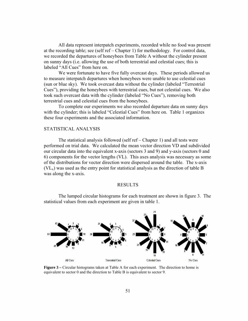
All data represent interpatch experiments, recorded while no food was present

at the recording table; see (self ref – Chapter 1) for methodology. For control data, we recorded the departures of honeybees from Table A without the cylinder present on sunny days (i.e. allowing the use of both terrestrial and celestial cues; this is labeled “All Cues” from here on.

We were fortunate to have five fully overcast days. These periods allowed us to measure interpatch departures when honeybees were unable to use celestial cues (sun or blue sky). We took overcast data without the cylinder (labeled “Terrestrial Cues”), providing the honeybees with terrestrial cues, but not celestial cues. We also took such overcast data with the cylinder (labeled “No Cues”), removing both terrestrial cues and celestial cues from the honeybees.

To complete our experiments we also recorded departure data on sunny days with the cylinder; this is labeled “Celestial Cues” from here on. Table 1 organizes these four experiments and the associated information. STATISTICAL ANALYSIS

The statistical analysis followed (self ref – Chapter 1) and all tests were performed on trial data. We calculated the mean vector direction VD and subdivided our circular data into the equivalent x-axis (sectors 3 and 9) and y-axis (sectors 0 and 6) components for the vector lengths (VL). This axes analysis was necessary as some of the distributions for vector direction were dispersed around the table. The x-axis (VLx) was used as the entry point for statistical analysis as the direction of table B was along the x-axis.

RESULTS

The lumped circular histograms for each treatment are shown in figure 3. The statistical values from each experiment are given in table 1.

Figure 3 – Circular histograms taken at Table A for each experiment. The direction to home is equivalent to sector 0 and the direction to Table B is equivalent to sector 9.

51

Table 1 – The four experiments performed with their statistical data and sources of information available to the honeybees. VD represents the mean vector direction, VLx represents the mean x-axis component of the vector length; both are reported as the “mean ± SE”. The sample size (n) is reported as “number of trials, departures per trial”. The direction to Table B is 270º.

Experiment VD VLx n

All Cues 262.3 ± 4.9 0.514 ± .03 12, 20

Terrestrial Cues 262.3 ± 8.2 0.541 ± .03 6, 20

Celestial Cues 270.0 ± 9.4 0.300 ± .04 20, 10

No Cues 170.2 ± 36.6 0.051 ± .07 10,10

STATISTICAL TESTS OF INDIVIDUAL EXPERIMENTS

The vector direction (VD) from Table A to Table B was 270° for all experiments. Using one-sample t-tests, we conclude the departure directions from the All, Terrestrial, and Celestial Cues experiments were not statistically different from 270° (p > 0.05), while the No Cues experiment was marginally statistically different (p = 0.023). These data are summarized in the second column of Table 2. The x-axis component of the vector length (VLx from here on) was expected to be positive and different than 0. Using one sample t-tests, we conclude the All, Terrestrial, and Celestial Cues experiments were statistically different from 0 and positive (p < 0.001), while the No Cues experiment was not statistically different from 0, indicating randomness (p = 0.489). These data are summarized in the third column of Table 2. Table 2 – Associated p-values from one-sample t-tests for each experiment, depending upon the specific null hypothesis (different columns).

Experiment VD = 270 VLx = 0

All Cues 0.143 < 0.001

Celestial Cues 0.397 < 0.001

Terrestrial Cues 0.997 < 0.001

No Cues 0.023 0.489

STATISTICAL COMPARISONS OF EXPERIMENTS

52

We performed two-sample t-tests for similarity of each pair of experiments and summed the results in Table 3. From these tests we need to highlight the specific tests where the presence and absence of terrestrial cues were compared. For the vector direction (VD), the two most important comparisons are the All vs. Celestial Cues and the Terrestrial vs. Celestial Cues; these are marked with an asterisk in Table 3. In neither case is the VD statistically different, indicating the honeybees were able to choose the proper direction, with or without terrestrial cues.

For the x-component of the vector length (VLx), it is useful to compare all pairs. First, when terrestrial cues were present (All vs. Terrestrial Cues), there is no difference between the two and the VLx values are the highest. Second, all other comparisons are statistically different from each other (p ≤ 0.007), indicating that changes in the availability of navigational cues causes changes in the measurement of vector length. The specific trend observed here is that terrestrial cues give the highest vector lengths (All vs. Terrestrial Cues), only celestial cues being slightly lower (Celestial Cues) and when all cues are gone (No Cues) the vector length is not statistically different than 0 (Figure 4).

Table 3 –Associated p-values from two-sample t-tests for each pair of experiments. The non-shaded p-values are for VD tests and the shaded p-values are for VLx tests; the null hypothesis for both tests is no difference. The values with an asterisk compare the availability terrestrial cues to the lack of terrestrial cues.

Experiment All Cues Terrestrial Cues Celestial Cues No Cues

All Cues X 0.529 < 0.001 < 0.001

Terrestrial Cues 0.998 X < 0.001 < 0.001

Celestial Cues 0.473* 0.547* X 0.007

No Cues 0.034 0.037 0.025 X

53

Figure 4 – The x-axis component of the mean vector length (VLx) of all four experiments. The error bars indicate the standard error of the mean002E

DISCUSSION

The research presented here unambiguously demonstrates that terrestrial cues are not necessary when honeybees choose their interpatch departure directions; instead, celestial cues alone are sufficient. The Celestial Cues experiment reported a VD that was not significantly different from the expected 270° and a vector length that was significantly different from random. We can also finally put to rest the arguments that landmark theory is an all inclusive theory (Cartwright and Collett 1982) and formally expand our knowledge. With that being said, we cannot undermine the importance of terrestrial cues. When terrestrial cues were present, the vector lengths (measuring the accuracy of their decision making) were significantly higher than when terrestrial cues were not present. Hence, the terrestrial cues provide information with the highest amount of utility for decision making. NEW ADDITIONS TO THE HONEYBEE PLACE MAP

We now know that inside the honeybee mind resides a cognitive understanding of the locations of multiple places, independent of the terrestrial environment. These locations are mentally represented in the same reference frame and linked by at least one variable, the interpatch direction. This knowledge can be described as an interpatch direction linked place map, in addition to the previously mentioned characteristics of their place map(self reference – Chapters 1 and 2). MORE EXPERIMENTAL POWER

54

No previous experiment has adequately separated the different sources of information as we do here. With this ability comes detailed data. From Figure 4, we are able to see the influence of each navigational cue. In this context, terrestrial cues were just as effective as all possible cues, indicating a predominance of terrestrial cues over celestial cues. However, even in this context, celestial cues were better than no cues at all. There is no reason to believe this hierarchy is true for all cases. In another context, specifically where the interpatch distance is much greater, hierarchy of cue preference may be altered or even reversed. Modifications to this experimental design could easily investigate these problems. Another interesting aspect of this research is that we were able generate random departures by successfully eliminating the set of necessary navigational cues (No Cues). Therefore, we eliminate many arguments of other types of potential cues the honeybees could have used; specifically egocentric cues (if no food turn right 90°) and any celestial cues that penetrate clouds or any systematic error related to our recording device. Modifications of this design will allow investigation of these types of cues and the following questions: When are they removed? What types of stimuli are able to remove them (different sized cylinder, partial covers, etc.)? At this point, we strongly recommend that this data not be interpreted that honeybees do not possess egocentric navigational capabilities or that they cannot use celestial cues that penetrate clouds. DIFFICULTIES IN THIS RESEARCH The data reported here was troublesome to obtain, on many levels. The major obstacle was training the honeybees to forage inside the cylinder. When you learn to work with honeybees, you learn they like light for orientation purposes. Quite often, we would have to retrain the honeybees to enter the cylinder as many would sit and wait for the food to be alternated back to Table B. This disruption forced us to take data from only one table (2 cylinders may have been too disturbing for the honeybees), as well as increase the time between food alternations on occasion. We are confident this reliance on a single table did not disrupt our goals as no previous experiments showed major differences when both tables were compared and we have tried many food alternation times, exceeding our largest alternation times used here. On top of this difficulty, we had to limit data collection to one departure every 10 seconds to ensure data independence, while limiting the number of departures per trial to 10. The combination of this time distinction, the times when few honeybees were flying, and when they refused to go into our cylinder led us to longer and longer trial times. Given this difficulty, the data presented here is still quite statistically robust. LOOKING AHEAD

55

With more detailed analysis, provided by our method (self ref – Chapter 1), we get a more detailed understanding of the honeybee. The extent of honeybee cognition has yet to be realized, with our previous knowledge an embarrassing underestimate.

56

Chapter 4

Investigating Route Theory Route Knowledge Route theory states that honeybees are capable of interpatch foraging because they have a planned route they follow. This theory is more or less an extension of within-patch foraging when visiting individual flowers. It has been shown that in such contexts various insects avoid revisiting previously visited flowers by flying a consistent path to different flowers (Comba 1999). Tests of honeybee route knowledge consist of laboratory experiments (Zhang et al. 2000) and field experiments (Gross et al. 2009). Many previous experiments set up multiple feeding locations, usually in a small area; we wanted to extend this testing to a larger area to be sure we were testing interpatch contexts. These previous experiments were more interested in quantifying how honeybees would choose a route out of many feeding locations. We wanted to know if honeybees could learn experimentally defined sequences of food availability, maximizing their resource gain based upon these sequences. To make the terminology clearer, previous research analyzed generalized honeybee specified routes, whereas we analyze specific sequence understanding by forcing the sequence through training. Training Sequence Knowledge. Training is simple when testing if honeybees can learn a specific sequence. One need only pick a sequence and move a single feeder of food along the sequence. In general, movement of food should occur every 10 minutes from one location to the next. The research below describes sequences that involve linear, triangular, and rectangular constellations of feeding sites.

Study 4 - “The Traveling Salesman meets the Traveling Consumer: Sequence Understanding and Extrapolation in Honeybees (Apis mellifera)

When the Rules Change. We were able to use the end of one summer to run some pilot experiments based upon one of our sequence experiments (Rectangular – Figure 8 experiment). After two months of training this sequence we change the sequence to random. Here, the bees reverted to win-stay strategy as described above, but they also avoided the previous sequence. We have not gone into any detail here as it was marginal data, with few trials and based upon little training, giving us low confidence in the data. However, given what we did have, there is indication that the honeybees understood that the sequence rules had changed, and they should try the other options rather than

57

follow the nullified previous Figure 8 rules. An experiment could easily be designed to test this possibility in the future. Regardless, honeybees are quite capable of understanding sequences.

58

The Traveling Salesman meets the Traveling Consumer: Sequence Understanding and Extrapolation in Honeybees (Apis mellifera)

Danny Najera, Tyrun Flaherty, Phillip Grupe, Casey Guccione, Rudolf Jander

INTRODUCTION

Every traveling salesman has a problem to solve. How can they maximize

their sales, given locations that are spatially separated, while using the minimum amount of resources (typically for travel) to do so? The answer is not always simple, but typically involves visiting all locations in a predetermined sequence.

Honeybees are not salesmen, but instead they are consumers. These honeybees are presented with a similar problem, however. How can they maximize the amount of resource they can gather when their food sources (flowering plants) are both spatially separated and temporally limited, while using the minimum amount of resources to do so? Some researchers have looked at within patch sequences of honeybees (need reference), but in these cases there is little difference in the temporal availability of these resources. What is eventually measured is the sequence that honeybees choose (traplining), based upon the available resources.

Here we present research that demonstrates both spatial and temporal understanding of the availability of resources. In these cases, we experimentally define a specific sequence for the food availability of the resources, in an interpatch context, and test whether the honeybees can understand the sequence. If they do understand this sequence, they should be able to predict which location, out of more than one, should have food next, based upon the location that last had food available.

GENERAL EXPERIMENTAL INFORMATION

Location and General Training

The two experiments involving 3 tables are summarized here but presented in full in the Master’s Thesis of Tyrun Flaherty. All experiments were performed on the western campus of the University of Kansas during summer months. Honeybees were trained away from the hive using Von Frisch’s (1967) method of incrementally moving an artificial feeder filled with scented sugar water to a desired location. To promote interpatch foraging we alternated the food availability between the various locations as described in (self reference – Chapter 1). Data Collection and Statistical Measures All data collection involved recording interpatch departure directions as described in (self reference – Chapter 1). Briefly, we used a circular recording table to determine site specific departure directions as honeybees flew past the perimeter of the table through numbered sectors (30° each).

59

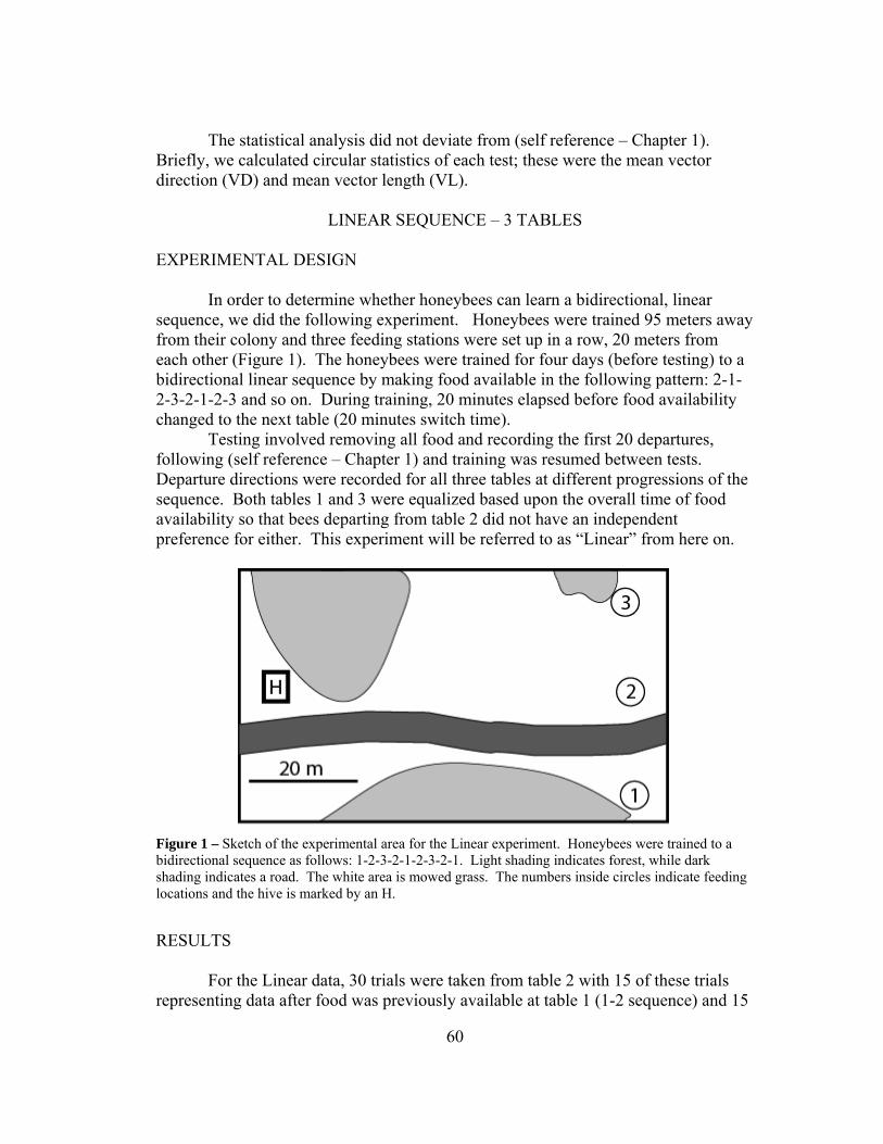
The statistical analysis did not deviate from (self reference – Chapter 1). Briefly, we calculated circular statistics of each test; these were the mean vector direction (VD) and mean vector length (VL).

LINEAR SEQUENCE – 3 TABLES

EXPERIMENTAL DESIGN

In order to determine whether honeybees can learn a bidirectional, linear sequence, we did the following experiment. Honeybees were trained 95 meters away from their colony and three feeding stations were set up in a row, 20 meters from each other (Figure 1). The honeybees were trained for four days (before testing) to a bidirectional linear sequence by making food available in the following pattern: 2-1-2-3-2-1-2-3 and so on. During training, 20 minutes elapsed before food availability changed to the next table (20 minutes switch time).

Testing involved removing all food and recording the first 20 departures, following (self reference – Chapter 1) and training was resumed between tests. Departure directions were recorded for all three tables at different progressions of the sequence. Both tables 1 and 3 were equalized based upon the overall time of food availability so that bees departing from table 2 did not have an independent preference for either. This experiment will be referred to as “Linear” from here on.

Figure 1 – Sketch of the experimental area for the Linear experiment. Honeybees were trained to a bidirectional sequence as follows: 1-2-3-2-1-2-3-2-1. Light shading indicates forest, while dark shading indicates a road. The white area is mowed grass. The numbers inside circles indicate feeding locations and the hive is marked by an H.

RESULTS For the Linear data, 30 trials were taken from table 2 with 15 of these trials representing data after food was previously available at table 1 (1-2 sequence) and 15

60

after food was previously available at table 3 (3-2 sequence); lumped histograms are reported in figure 2. For the 1-2 sequence, the VD was 71.87° ± 2.58° (mean ± SE) and the expected value was 90°. For the 3-2 sequence, the VD was 283.99° ± 2.56° (mean ± SE) and the expected value was 270°. In all cases, the modes were located in the expected sector and all vector lengths were significantly different than 0 (p < 0.001).

Figure 2 – Lumped histograms of departure directions for the Linear experiment. The dot in the histogram represents the expected direction and in all cases the mode of the data is directly in line with the expectation.

TRIANGLE SEQUENCE – 3 TABLES EXPERIMENTAL DESIGN

In order to determine whether honeybees can learn a circular sequence (using three tables arranged in a triangle), we did the following experiment. Honeybees were trained 45 meters away from their colony and three feeding stations were set up in an equilateral triangle with an inter-table distance of 20 meters (Figure 3). The honeybees were trained for five days (before testing) to a clockwise sequence by making food available in the following pattern: 4-5-6-4-5-6 and so on. During training 20 minutes elapsed before food availability changed to the next table. Testing involved removing all food and recording the first 20 departures, following (self reference – Chapter 1) and training was resumed between tests. Departure directions were recorded for all three tables. This experiment will be referred to as “Triangle” from here on.

61

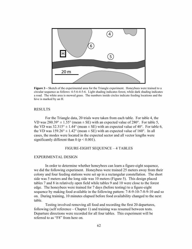
Figure 3 – Sketch of the experimental area for the Triangle experiment. Honeybees were trained to a circular sequence as follows: 4-5-6-4-5-6. Light shading indicates forest, while dark shading indicates a road. The white area is mowed grass. The numbers inside circles indicate feeding locations and the hive is marked by an H.

RESULTS For the Triangle data, 20 trials were taken from each table. For table 4, the VD was 280.39° ± 1.55° (mean ± SE) with an expected value of 280°. For table 5, the VD was 32.315° ± 1.44° (mean ± SE) with an expected value of 40°. For table 6, the VD was 159.26° ± 1.42° (mean ± SE) with an expected value of 160°. In all cases, the modes were located in the expected sector and all vector lengths were significantly different than 0 (p < 0.001).

FIGURE-EIGHT SEQUENCE – 4 TABLES

EXPERIMENTAL DESIGN

In order to determine whether honeybees can learn a figure-eight sequence, we did the following experiment. Honeybess were trained 25 meters away from their colony and four feeding stations were set up in a rectangular constellation. The short side was 5 meters and the long side was 10 meters (Figure 5). This design placed tables 7 and 8 in relatively open field while tables 9 and 10 were close to the forest edge. The honeybees were trained for 7 days (before testing) to a figure-eight sequence by making food available in the following pattern: 7-8-9-10-7-8-9-10 and so on. During training, 10 minutes elapsed before food availability changed to the next table. Testing involved removing all food and recording the first 20 departures, following (self reference – Chapter 1) and training was resumed between tests. Departure directions were recorded for all four tables. This experiment will be referred to as “F8” from here on.

62

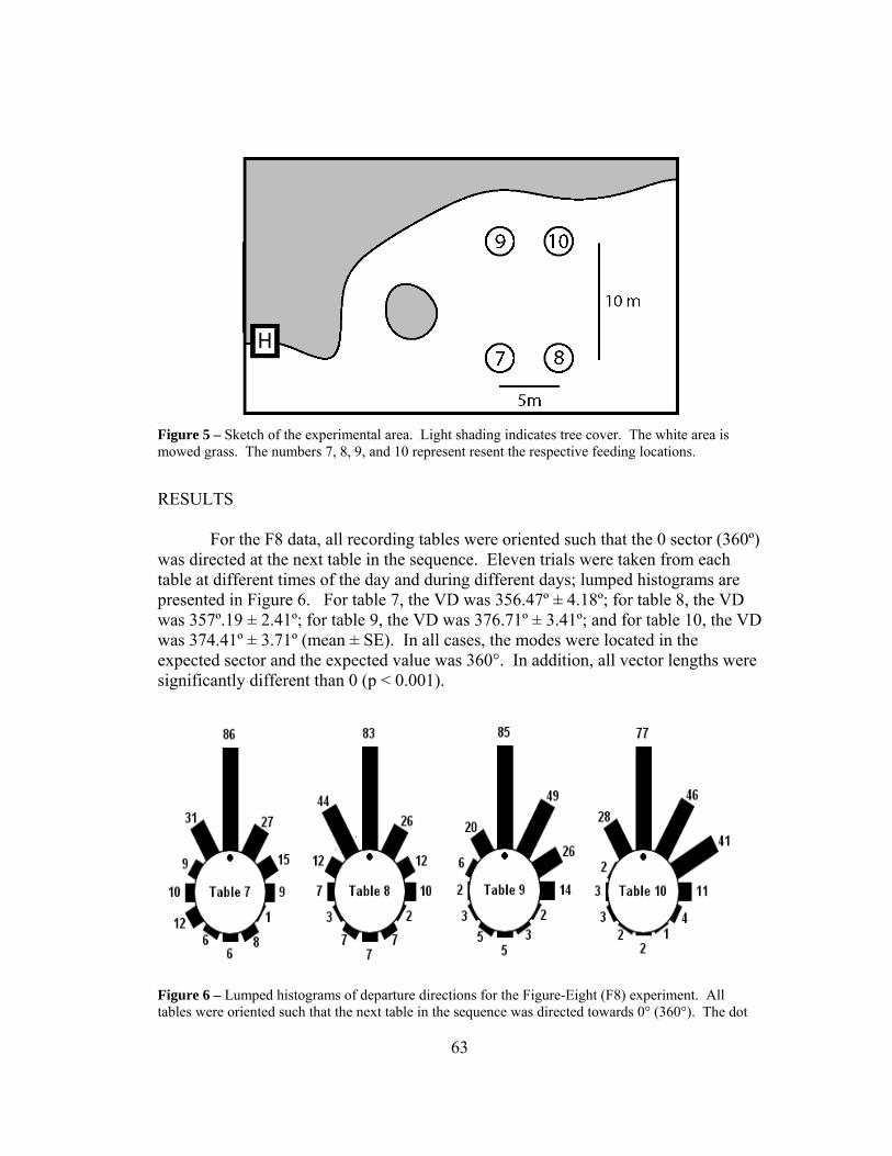
Figure 5 – Sketch of the experimental area. Light shading indicates tree cover. The white area is mowed grass. The numbers 7, 8, 9, and 10 represent resent the respective feeding locations.

RESULTS For the F8 data, all recording tables were oriented such that the 0 sector (360º) was directed at the next table in the sequence. Eleven trials were taken from each table at different times of the day and during different days; lumped histograms are presented in Figure 6. For table 7, the VD was 356.47º ± 4.18º; for table 8, the VD was 357º.19 ± 2.41º; for table 9, the VD was 376.71º ± 3.41º; and for table 10, the VD was 374.41º ± 3.71º (mean ± SE). In all cases, the modes were located in the expected sector and the expected value was 360°. In addition, all vector lengths were significantly different than 0 (p < 0.001).

Figure 6 – Lumped histograms of departure directions for the Figure-Eight (F8) experiment. All tables were oriented such that the next table in the sequence was directed towards 0° (360°). The dot

63

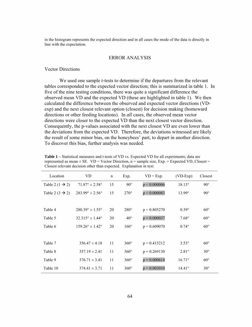
in the histogram represents the expected direction and in all cases the mode of the data is directly in line with the expectation.

ERROR ANALYSIS

Vector Directions We used one sample t-tests to determine if the departures from the relevant tables corresponded to the expected vector direction; this is summarized in table 1. In five of the nine testing conditions, there was quite a significant difference the observed mean VD and the expected VD (these are highlighted in table 1). We then calculated the difference between the observed and expected vector directions (VD-exp) and the next closest relevant option (closest) for decision making (homeward directions or other feeding locations). In all cases, the observed mean vector directions were closer to the expected VD than the next closest vector direction. Consequently, the p-values associated with the next closest VD are even lower than the deviations from the expected VD. Therefore, the deviations witnessed are likely the result of some minor bias, on the honeybees’ part, to depart in another direction. To discover this bias, further analysis was needed. Table 1 – Statistical measures and t-tests of VD vs. Expected VD for all experiments; data are represented as mean ± SE. VD = Vector Direction, n = sample size, Exp. = Expected VD, Closest = Closest relevant decision other than expected. Explanation in text

Location VD n Exp. VD = Exp. (VD-Exp) Closest

Table 2 (1 2) 71.87° ± 2.58° 15 90° p < 0.000006 18.13° 90°

Table 2 (3 2) 283.99° ± 2.56° 15 270° p < 0.000083 13.99° 90°

Table 4 280.39° ± 1.55° 20 280° p = 0.805270 0.39° 60°

Table 5 32.315° ± 1.44° 20 40° p = 0.000037 7.68° 60°

Table 6 159.26° ± 1.42° 20 160° p = 0.609070 0.74° 60°

Table 7 356.47 ± 4.18 11 360° p = 0.415212 3.53° 60°

Table 8 357.19 ± 2.41 11 360° p = 0.269130 2.81° 30°

Table 9 376.71 ± 3.41 11 360° p = 0.000614 16.71° 60°

Table 10 374.41 ± 3.71 11 360° p = 0.003010 14.41° 30°

64

Direction of Observed Deviations from Expected In all cases, there were deviations in the observed VD and the expected VD.

When we plot these deviations on the maps of the testing areas, we notice a consistent trend. Specifically, all deviations are in the direction of the hive. We chose the figure-eight (F8) experiment to go into detail here, but the same could be done for the other two experiments (Linear and Triangle). The analysis is as follows. If we look at the vector directions of all four tables (7, 8, 9, and 10), they all have deviations from the expected VD of 360º. For tables 7 and 8, these deviations are relatively small and for tables 9 and 10, these deviations are relatively large; figure 7a displays the deviations, relative to their expected directions. Interestingly enough, these deviations all point towards a common area. This common area must have some excitatory cue, causing the deviations. Within this common region is the hive. This analysis is described in figure 7.

Figure 7 – a) Departure directions from the four tables 7, 8, 9, and 10. The dashed lines indicate expected departure directions and the solid lines with arrowheads represent the deviated, observed departure directions. b) Each of the directional deviations from the four tables indicated a preference in direction relative to the expected direction. We extended these expected direction lines to the edge of the map and colored the area that to the side of the deviation. Specifically we colored below line I, above line II, to the left of line III and to the left of line IV. These shaded areas all overlapped to one area which we left shaded above. The deviations can be explained by some excitatory stimulus (the hive) found in this region. Light shade indicates tree cover.

SYSTEMATIC ERRORS AND THEIR REMOVAL

We must be careful because our data came in the form of group data and from one table at a time, therefore, we must account for two possible systematic errors. The first is that there may be subgroups of honeybees that always depart from the same table, and in the correct direction. This systematic error is handled in the “pseudo-mark-recapture data” section below. The second is that we have not shown that any honeybee has complete path sequence knowledge. This systematic error is handled in the “individual data” section below.

65

Pseudo-Mark-Recapture Are there subgroups of bees that only need to know small segments of the sequence? First and foremost, if this were the case, this solution would be an interesting way for groups of honeybees to solve sequence problems, displaying an group selected foraging strategy. To account for this possibility we performed a pseudo-mark-recapture study. While honeybees were feeding at one of the feeding sites, we painted a specific number of them a single color. The next day we then counted the number of painted to non-painted honeybees at all feeder locations and at different times of the day; this was done for all 3 experiments above. In all cases, there was no statistical difference in the proportion of painted to non-painted bees (p > 0.05). In no case did we find evidence of subgroups; this holds true for many other experiments we have performed. Individual Data Are individuals capable of learning sequence information to maximize their foraging efficiency? To account for this possibility we trained honeybees to a figure-eight pattern in a different year than the F8 experiment above. After a week of sparse training, we painted honeybees to make them individually recognizable. We then tracked the tables that they visited by using 4 observers, one at each table. We then recorded when specific individuals arrived at specific tables, and followed them visually as they flew from table to table. We then gathered their sequences and compared each decision, relative to the expected correct decision. For any given table, the honeybees could make a correct decision, flying to the next table in sequence (only one possibility), or an incorrect decision, flying to either of the other two tables. Therefore, when making a decision there were 3 possibilities, 1 correct decision (33%) and 2 incorrect decisions (66%). We then used a binomial test with the respective probabilities (0.33 for correct and 0.66 for incorrect) to test if the honeybees were making better than random decisions. We found multiple individuals were making decisions better than random, with two individuals that completed more than 50 decisions (n = 80 and 60); these individuals provided the most robust information as their sample sizes were the two highest; the proportions of correct decisions for these honeybees were 0.59 (47/80) and 0.47 (28/60) and the associated binomial p-values (null hypothesis of 0.33) are p < 0.001 and p = 0.038 respectively. Individuals have the ability learn sequences and fly appropriately to most efficiently gather resources, even when the correct table was the furthest away. While we do not have data for the other two experiments (Linear and Triangle), we recognize that these are more simplistic sequences and fully expect that individual honeybees are easily making these decisions.

CONCLUSIONS

66

Honeybees can learn experimentally defined sequences. We demonstrate three qualitatively different sequences: a bidirectional sequence (Linear), a circular sequence (Triangle) and a figure eight sequence (F8). Unique to this research, each of these sequences was learned in an interpatch context while foraging under natural conditions. These findings add to the already well documented route knowledge found in honeybees (need reference). The Analysis of Context While the decision making of these honeybees was qualitatively distinct, the qualitative measurements showed some interesting differences when compared to what we expected. Even though there were slight, but significant deviations, this bias did not imply that honeybees were choosing the other directions (table 1).

When we further analyzed the data, we were able to come up with a plausible explanation for all deviations found in these experiments; the colony acted as an excitatory stimulus, slightly biasing the direction of departure. However, these experiments were not designed to take advantage of this fine level of analysis to be sure that it was the colony. In fact, we noticed some interesting trends when tables were located close to trees, specifically in the vector lengths (not reported here); this has been noticed previously (self reference – Chapter 2). The experimental method used here and more thoroughly described in (self reference – Chapter 1) is fully capable of dealing with these fine details. In fact, we have some observations that moving a recording table only 1 meter can significantly alter the departure directions of honeybees. The reasons for such significant deviations, like in this paper, remain somewhat hidden. In time, we fully expect to determine which cues, in the natural environment, can be excitatory and inhibitory. Pseudo-Mark-Recapture In this paper we introduce another powerful technique used to account for systematic errors in our experiment. When analyzing multiple decisions made by organisms, specifically when taking group data, one needs to be sure that there are not subgroups of individuals within the group. We present an effective way to remove this systematic error using the principles of mark-recapture techniques. Throughout many experiments where such pseudo-mark-recapture has been performed, we have never found evidence that there are subgroups of foraging honeybees giving our familiarity training (self reference - Chapter 1). Additions to the Place Map Given the research presented here, we can now state that for the place map of honeybees, places are capable of being linked together based upon sequential knowledge. While route knowledge has been show previously (need references), this data is the first explicit demonstration of it using interpatch foraging techniques (self

67

reference – Chapter 1). Also, we were able to experimentally define a sequence that the honeybees were able to learn and use predictively. We therefore add a sequence-able quality to the honeybee place map with respect to interpatch foraging. We expect that such sequence knowledge is stored in long term memory, as 40 minutes passed in a cycle for the F8 experiment, though we did not test the type of memory directly. It is through small and calculated details that organisms are efficient. Here, the traveling consumer (honeybees) pays close attention to its resources, the same way the traveling salesman pay attention to his buyers. With the goal of maximizing their efforts, they plan specific sequential strategies and get to work. One can only begin to wonder how many locations these honeybees are capable of arranging sequentially.

68

Chapter 5

Challenging Route Theory How to Challenge Route Theory The route knowledge (or uni-dimensional flight sequence) of honeybees is well demonstrated and quite complex (chapter 4). However, just like landmark theory, route knowledge has been implicated as being necessary and sufficient for interpatch foraging (Wehner and Wehner 1990). In the following set of experiments we aimed to challenge this theory directly. Route theory has been explicitly redesigned as a contrast to the cognitive map theory. Specifically, it is theorized that the extent of honeybee route knowledge be one-dimensional and serial. The one-dimensional aspect is necessary as a contrast to 2-dimensional (or greater) knowledge of places, typical of conventional maps (cognitive and not); we address this issue in chapter 6. The serial aspect is necessary as the historical belief is that foraging decisions are made in the colony and outside the route is simply followed; this is addressed below. Each of these aspects can be directly linked back to the belief that the waggle dances are the extent of the of honeybees knowledge. The Hive as a Hub Many of the classical experiments defined the knowledge base of the honeybee from the colony using outward and homing paths (paths linked to the colony itself). Such studies include knowledge about circadian times, compass directions, flight distances, site specific utility, and site specific stimulus characterization (Frisch 1967, Wahl 1932, Lindauer 1960). This knowledge is ecologically relevant as it increases the foraging efficiency, and in turn, the survivability of the colony. Add on top of this knowledge the waggle dances, which served as the mechanism to obtain much of this information, and the degree of complexity in such a small insect is astounding. Thus, the hive can be considered as a hub of knowledge, a central location from which decisions were made.

Unfortunately this knowledge, which is foundational to colony survival, was not extended beyond the location of colony. Once the bee left the colony it was once again a stupid insect. It could not apply similar knowledge in other places, and it could not learn about such things without reference to the colony; this hub was sacred and unique. Beacon orientation, Landmark theory, and Route theory were constructed to once again minimize the cognitive power of honeybees; even with the massive amount of information just discovered inside the colony. We argue that the cognitive abilities of honeybees are not inherently reduced once they leave their home; qualitative cognitive abilities are not place specific. This idea needed to be challenged and the experimental methods to do so are described below.

69

Secondary Hubs Is it possible that a location other than the colony can function as a hub as well? If so, our first assumption would be the colony is the most important or primary hub, if only for the reason that it is the location that any given honeybee spends the most time at. We also expect that other potential hubs will exhibit many characteristics of primary hubs, but would lack some specific details; these are referred to as secondary hubs. Fortunately, there is a well known context in which the concept of a secondary hub could be used; this is in the context of swarming. This research has primarily been led by (Robinson and Dyer 1993). Here, the swarm must be informed and make informed decisions. Based upon this data, some individuals share time between the original colony and the newly congregated swarm, while searching for new locations for the swarm (Robinson and Dyer 1993). These individuals must juggle two different hubs in their mind. For our purposes, however, these would both be primary hubs as the concept of “home” would apply to both even though the swarm is temporary or intermediate. One characteristic these two primary hubs have in common is the waggle dance. In fact, most of the information from swarms, in this context, has come from the waggle dance. We needed to develop a different strategy that would allow us to address this issue, as swarms were too similar to established colonies. Stimulus Dependent Decision Making Outside of the Hive As route theory was used to explain interpatch foraging, we needed to use a foraging site as a potential secondary hub and use the context of interpatch foraging. We would then have to have a specific location where we could test decision making to determine if honeybees are able to make decisions at this secondary hub, similar to the colony decisions (primary hub). In all experiments described in this chapter, this potential secondary hub is referred to as the center table. To measure interpatch decision making (with respect to foraging), we must use stimuli that are either associated with the rewards (linked stimuli) or have a better than 0 chance of predicting the location of rewards (predictive stimuli). Each option must also be distinguishable from eachother. In the research below, we used odor cues that were linked and predictive, color cues that were predictive, and temporal cues that were linked. All were learned quite thoroughly, showing that honeybees can make well informed decisions while foraging outside the colony. Here, no pre-established routes (from the colony) could guide their knowledge. Therefore, just like landmark theory, route theory describes one strategy that honeybees can use, but are not limited to. Neither landmark theory, nor route theory, describes the full extent of honeybee cognition used in foraging.

Study 5 - “Secondary Hubs in Honeybees: Demonstration of Branching Interpatch Decision Making”

70

Initial Tests: Long-term Memory vs. Short-Term Memory Familiarity training provides us with repetitive testing. As illustrated above, with the repetition, a honeybee experiences our experiments day after day. This familiarity allows us to test their long-term memory and their short-term memory separately. While foraging actively during the day, each honeybee experiences stimuli, learns patterns, and stores this information in short-term memory. As we test during the day we potentially test both long-term memory (from the day before) and short-term memory (from that day). Over the night, the short-term memory must be converted into long-term memory and recalled the following morning. These initial tests, before experience on that day, specifically test long-term memory. We can compare the difference between initial tests and subsequent tests for a comparison of long-term and short-term memory. In this research, we found no differences to the extent of making completely different decisions. We expect that for some stimuli in some specific contexts, there will be such massive differences. Finishing Direction Knowledge Everything up to this point has dealt with interpatch foraging, only involving interpatch direction knowledge. With both landmark theory and route theory representing only part of the cognitive repertoire we had to address the final option, the cognitive map. However, instead of repeating the historical mistake (trying to verify a confused concept) we sought to determine if honeybees had complete interpatch vector knowledge. So began the quest for investigating interpatch distance knowledge, fundamentally requiring more methodological creativity.

71

Secondary Hubs in Honeybees Navigation: Demonstration of Branching Interpatch Decision Making

Erin McCullough, Tyrun Flaherty, Patty Van Meter, Liz Munz, Danny Najera, Rudolf

Jander

INTRODUCTION

All central-place foragers travel, at minimum, three fundamentally different foraging paths: outward paths (home to patch), the homeward or homing paths (patch to home) and interpatch paths (patch to patch). Bees are well known to travel such interpatch paths in natural contexts (Seeley 1985, Comba 1999) as well as experimentally designed contexts (Greggers and Menzel 1993, self reference – Chapter 1, 2, 3, and 4). Previous explanations of interpatch foraging required that honeybees either used conspicuous terrestrial landmarks (Cartwright and Collett 1982, 1987), followed prescribed routes (Dyer 1991, Wehner and Wehner 1990), or used a diverse range of cognitive mapping mechanisms (Gould 1986). Self reference - Chapter 3 was able to show that landmark theory was only a subset of a much richer foraging knowledge as honeybees were shown to make informed decisions in the absence of any terrestrial landmark stimuli; celestial stimuli alone were sufficient in guiding these decisions. We wanted to challenge route theory in a similar fashion, to see if it honeybee foraging knowledge could be adequately explained by the use of prescribed routes alone. To understand the is sue more clearly, we need to start with the knowledge base of honeybees as defined by their home, the hive. Hubs and Interpatch Decision Making Theory

Many of the classical experiments defined the knowledge base of the honeybee from the hive using outward paths and dance communications. Such studies include knowledge about circadian times, compass directions, flight distances, site specific utility, and site specific stimulus characterization (Von Frisch 1967, Wahl 1932, Lindauer 1960). Thus, the hive can be considered as a primary hub of knowledge, a central location from which decisions are made.

Route theory specifies that from the hive, foraging decisions encompass complete routes, thus making the route serial (one-dimensional) and non-branching. Inclusive to this theory is the assumption that such informed decision making (as mentioned above) cannot be accomplished outside of the hive. If we remove this assumption, we should expect that a similarly rich knowledge applies while honeybees are foraging, outside the hive. We could imagine that similarly well informed interpatch decisions are made at secondary hubs (familiar locations not associated with the concept of home) to maximize resource gain.

From these theoretical secondary hubs, the absence of food would initiate branching interpatch decisions, utilizing at least two types of stimuli: predictive and linked stimuli. We define a predictive stimulus as any stimulus present at a

72

secondary hub that provides a better than zero chance of indicating how to find an auxiliary location with food. Such predictive stimuli are similar to signposts or guides, but not present at the auxiliary location itself. We define a linked stimulus as any stimulus present at a secondary hub that is also found at the auxiliary location with food; such linked stimuli are likely to be linked directly to the food source itself (nectar qualities, plant characteristic, etc.) although it is not necessary.

Here, we perform multiple experiments designed to investigate if route theory is sufficient to explain observable honeybee foraging. These experiments seek to identify potential secondary hubs, display branching decision making, and test both types of stimuli (predictive and linked).

GENERAL METHODS

Location and Materials All experiments were performed during the summer months on the west campus of the University of Kansas, Lawrence, Kansas. Honeybees were trained away from the hive using von Frisch’s (1967) method of incrementally moving an artificial feeder filled with scented sugar water to a desired location. To promote interpatch foraging we alternated the food availability between two locations at a time as described in (self reference - Chapter 1). All data collection involved recording homing and interpatch departure directions as described in (self reference – Chapter 1). Briefly, we used a circular recording table to determine site specific departure directions as honeybees flew past the perimeter of the table through numbered sectors (30º each). All odors came from adding food flavoring extracts to water or sugar water. Terminology We use specific terminology here to refer to our different locations. A primary hub is a location at which foraging decisions can be made and the concept of home can be applied (this context can be the hive or a swarm (Seeley 1985). A secondary hub is a location at which branching foraging decisions can be made and the concept of home cannot be applied. All other relevant locations in these experiments are referred to as auxiliary sites. Statistics The statistical analysis did not deviate from (self references - Chapter 1). Briefly, we calculated the circular statistics of each test: these are the mean vector direction (VD) and mean vector length (VL). As necessary, we decomposed the vector length quantities into their axial components with the x-axis (VLx) being perpendicular to the home direction and the y-axis (VLy) being in the same direction to the home direction. These statistics (VD, VLx, and VLy) were then used as entry

73

points for statistical analysis. For comparisons to expected values or comparisons of data sets to each other we used t-tests to evaluate our various null hypothesis.

In all situations where we measured homeward departures, the data were distributed towards home (p > 0.05) and significantly different than directions to all other locations (p < 0.00001) as expected from many previous experiments using this method (self reference – Chapters 1, 2, 3, and 4).

EXPERIMENT 1 - PREDICTIVE ODOR STIMULI Experimental Design

In order to determine whether honeybees can make branching interpatch decisions from a secondary hub based on predictive odor stimuli, we trained honeybees to forage between a central location (designated W) and two auxiliary feeders (designated 1 and 2). Location W was 100m away and the three locations were arranged in a linear path (figure 1a). Twenty meters separated location W from locations 1 and 2. At location W we set up a dish that we could add odor stimuli to. On top of this dish we placed sturdy wire mesh that prevented the bees from contacting the contents of the dish; this guaranteed that the stimuli were olfactory and not gustatory. The feeder was then placed on the top of the wire mesh. At auxiliary locations 1 and 2 we only had feeders filled with unscented sugar water.

Figure 1 – a) Sketch of the experimental area. Light shading indicates forest, while dark shading indicates a road. The white area is mowed grass. W, 1, and 2 represent the feeding locations. b) Decision making flow chart of the honeybee as it arrives at site W. If there is food, it feeds (becomes satiated) and goes home. If there is no food, it is hungry and must rely on the current stimulus to guide its next decision. If W smells like peppermint, then the honeybee should depart towards location 1; if lavender, location 2.

For training, we wanted location W to be the most consistently visited as we wanted to determine if branching interpatch decisions could be made from this location. Therefore we established a pseudo-random feeding regimen that alternated food availability (every 15 minutes) from the secondary hub (W) to the auxiliary sites (1 and 2). The randomness was necessary to avoid sequence learning as shown in (self reference – Chapter 4). It was a pseudo-random sequence in that we did not

74

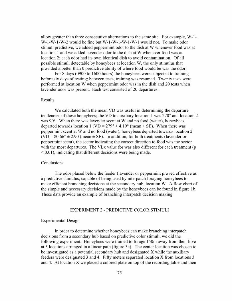
allow greater than three consecutive alternations to the same site. For example, W-1-W-1-W-1-W-2 would be fine but W-1-W-1-W-1-W-1 would not. To make odor stimuli predictive, we added peppermint odor to the dish at W whenever food was at location 1 and we added lavender odor to the dish at W whenever food was at location 2; each odor had its own identical dish to avoid contamination. Of all possible stimuli detectable by honeybees at location W, the only stimulus that provided a better than 0 predictive ability of where food would be was the odor.

For 8 days (0900 to 1600 hours) the honeybees were subjected to training before six days of testing; between tests, training was resumed. Twenty tests were performed at location W when peppermint odor was in the dish and 20 tests when lavender odor was present. Each test consisted of 20 departures. Results

We calculated both the mean VD was useful in determining the departure tendencies of these honeybees; the VD to auxiliary location 1 was 270° and location 2 was 90°. When there was lavender scent at W and no food (water), honeybees departed towards location 1 (VD = 279° ± 4.19° (mean ± SE). When there was peppermint scent at W and no food (water), honeybees departed towards location 2 (VD = 80.66° ± 2.90 (mean ± SE). In addition, for both treatments (lavender or peppermint scent), the sector indicating the correct direction to food was the sector with the most departures. The VLx value for was also different for each treatment (p < 0.01), indicating that different decisions were being made. Conclusions

The odor placed below the feeder (lavender or peppermint proved effective as a predictive stimulus, capable of being used by interpatch foraging honeybees to make efficient branching decisions at the secondary hub, location W. A flow chart of the simple and necessary decisions made by the honeybees can be found in figure 1b. These data provide an example of branching interpatch decision making.

EXPERIMENT 2 - PREDICTIVE COLOR STIMULI Experimental Design

In order to determine whether honeybees can make branching interpatch decisions from a secondary hub based on predictive color stimuli, we did the following experiment. Honeybees were trained to forage 150m away from their hive at 3 locations arranged in a linear path (figure 3a). The center location was chosen to be investigated as a potential secondary hub and designated X while the auxiliary feeders were designated 3 and 4. Fifty meters separated location X from locations 3 and 4. At location X we placed a colored plate on top of the recording table and then

75

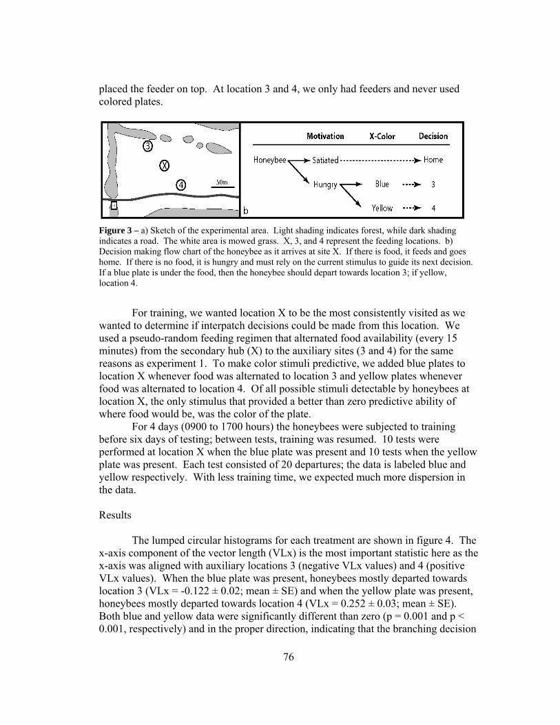
placed the feeder on top. At location 3 and 4, we only had feeders and never used colored plates.

Figure 3 – a) Sketch of the experimental area. Light shading indicates forest, while dark shading indicates a road. The white area is mowed grass. X, 3, and 4 represent the feeding locations. b) Decision making flow chart of the honeybee as it arrives at site X. If there is food, it feeds and goes home. If there is no food, it is hungry and must rely on the current stimulus to guide its next decision. If a blue plate is under the food, then the honeybee should depart towards location 3; if yellow, location 4.

For training, we wanted location X to be the most consistently visited as we

wanted to determine if interpatch decisions could be made from this location. We used a pseudo-random feeding regimen that alternated food availability (every 15 minutes) from the secondary hub (X) to the auxiliary sites (3 and 4) for the same reasons as experiment 1. To make color stimuli predictive, we added blue plates to location X whenever food was alternated to location 3 and yellow plates whenever food was alternated to location 4. Of all possible stimuli detectable by honeybees at location X, the only stimulus that provided a better than zero predictive ability of where food would be, was the color of the plate.

For 4 days (0900 to 1700 hours) the honeybees were subjected to training before six days of testing; between tests, training was resumed. 10 tests were performed at location X when the blue plate was present and 10 tests when the yellow plate was present. Each test consisted of 20 departures; the data is labeled blue and yellow respectively. With less training time, we expected much more dispersion in the data. Results The lumped circular histograms for each treatment are shown in figure 4. The x-axis component of the vector length (VLx) is the most important statistic here as the x-axis was aligned with auxiliary locations 3 (negative VLx values) and 4 (positive VLx values). When the blue plate was present, honeybees mostly departed towards location 3 (VLx = -0.122 ± 0.02; mean ± SE) and when the yellow plate was present, honeybees mostly departed towards location 4 (VLx = 0.252 ± 0.03; mean ± SE). Both blue and yellow data were significantly different than zero (p = 0.001 and p < 0.001, respectively) and in the proper direction, indicating that the branching decision

76

making is not random. In addition, for both Blue and Yellow data, the sector indicating the correct direction to food was the sector with the most departures. The VLx value for both Blue and Yellow data were also different from each other (p < 0.001) indicating that different decisions were being made.

Figure 4 – Histograms of branching decision making using predictive color stimuli (plates). The histogram with blue in the center represents data taken at location X with a blue plate under the feeder, while the histogram with yellow in the center represents data taken at location X with a yellow plate under the feeder. Location X can be considered a secondary hub where branching decisions are made. The black dot indicates the proper direction.

Conclusions

The color of the plate (blue or yellow) proved effective as a predictive

stimulus, capable of being used by interpatch foraging honeybees to make efficient branching decisions at the secondary hub, location X. A flow chart of the simple and necessary decisions made by the honeybees can be found in figure 3b. These data provide an example of branching interpatch decision making.

EXPERIMENT 3 - LINKED ODOR STIMULI Experimental Design

In order to determine whether honeybees can make branching interpatch decisions from a secondary hub based on linked odor stimuli, we did the following experiment. Honeybees were trained to forage 100m away from their hive at 2 locations labeled 5 and 6 arranged in (figure 5a). The distance between these locations was 20m. At location 5 we applied peppermint odor to the sugar water and at location 6 we applied lavender odor.

77

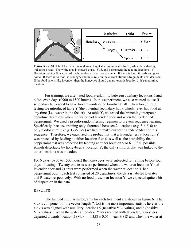
Figure 5 – a) Sketch of the experimental area. Light shading indicates forest, while dark shading indicates a road. The white area is mowed grass. Y, 5, and 6 represent the feeding locations. b) Decision making flow chart of the honeybee as it arrives at site Y. If there is food, it feeds and goes home. If there is no food, it is hungry and must rely on the current stimulus to guide its next decision. If the food smells like lavender, then the honeybee should depart towards location 5; if peppermint, location 6.

For training, we alternated food availability between auxiliary locations 5 and 6 for seven days (0900 to 1500 hours). In this experiment, we also wanted to test if secondary hubs need to have food rewards or be familiar at all. Therefore, during testing we introduced table Y (the potential secondary hub), which never had food at any time (i.e., water in the feeder). At table Y, we tested the branching interpatch departure directions when the water had lavender odor and when the feeder had peppermint. We used a pseudo-random testing regimen to prevent sequence learning. Specifically, because training only alternated between 2 locations (e.g. 5-6-5-6) and only 2 odor stimuli (e.g. L-V-L-V) we had to make our testing independent of this sequence. Therefore, we equalized the probability that a lavender test at location Y was preceded by feeding at either location 5 or 6 as well as the probability that a peppermint test was preceded by feeding at either location 5 or 6. Of all possible stimuli detectable by honeybees at location Y, the only stimulus that was linked to the other locations was the odor. For 6 days (0900 to 1500 hours) the honeybees were subjected to training before four days of testing. Twenty one tests were performed when the water at location Y had lavender odor and 21 tests were performed when the water at location Y had peppermint odor. Each test consisted of 20 departures; the data is labeled L-water and P-water respectively. With no food present at location Y, we expected quite a bit of dispersion in the data. RESULTS The lumped circular histograms for each treatment are shown in figure 6. The x-axis component of the vector length (VLx) is the most important statistic here as the x-axis was aligned with auxiliary locations 5 (negative VLx values) and 6 (positive VLx values). When the water at location Y was scented with lavender, honeybees departed towards location 5 (VLx = -0.358 ± 0.05; mean ± SE) and when the water at

78

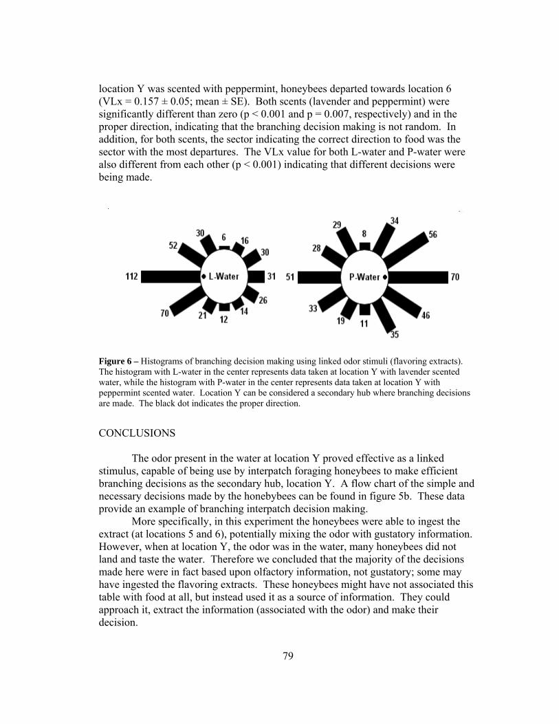
location Y was scented with peppermint, honeybees departed towards location 6 (VLx = 0.157 ± 0.05; mean ± SE). Both scents (lavender and peppermint) were significantly different than zero (p < 0.001 and p = 0.007, respectively) and in the proper direction, indicating that the branching decision making is not random. In addition, for both scents, the sector indicating the correct direction to food was the sector with the most departures. The VLx value for both L-water and P-water were also different from each other (p < 0.001) indicating that different decisions were being made.

Figure 6 – Histograms of branching decision making using linked odor stimuli (flavoring extracts). The histogram with L-water in the center represents data taken at location Y with lavender scented water, while the histogram with P-water in the center represents data taken at location Y with peppermint scented water. Location Y can be considered a secondary hub where branching decisions are made. The black dot indicates the proper direction.

CONCLUSIONS The odor present in the water at location Y proved effective as a linked stimulus, capable of being use by interpatch foraging honeybees to make efficient branching decisions as the secondary hub, location Y. A flow chart of the simple and necessary decisions made by the honebybees can be found in figure 5b. These data provide an example of branching interpatch decision making.

More specifically, in this experiment the honeybees were able to ingest the extract (at locations 5 and 6), potentially mixing the odor with gustatory information. However, when at location Y, the odor was in the water, many honeybees did not land and taste the water. Therefore we concluded that the majority of the decisions made here were in fact based upon olfactory information, not gustatory; some may have ingested the flavoring extracts. These honeybees might have not associated this table with food at all, but instead used it as a source of information. They could approach it, extract the information (associated with the odor) and make their decision.

79

EXPERIMENT 4 - LINKED TEMPORAL STIMULI

EXPERIMENTAL DESIGN

In order to determine whether honeybees can make branching interpatch decisions from a secondary hub based on linked temporal stimuli, to three other locations, we did the following experiment. Honeybees were trained to forage 100m away from their hive at four locations with the particular constellation shown in figure 7a. The center location was chosen to be investigated as a potential secondary hub and designated Z; the auxiliary feeders were designated 7, 8, and 9. Ten meters separated location Z from locations 7, 8, and 9. All locations were given vanilla odor (food and water) and contained a blue plate to facilitate any linkage of the four locations in the mind of the honeybees.

Figure 7 – a) Sketch of the experimental area. Light shading indicates forest, while dark shading indicates a road. The white area is mowed grass. Z, 7, 8, and 9 represent the feeding locations. b) Decision making flow chart of the honeybee as they arrive at site Z. If there is food, it feeds and goes home. If there is no food, it is hungry and must rely on the current stimulus to guide its next decision: if in the morning then the honeybee should depart towards location 7; if noon, location 8; if afternoon, location 9.

For training we needed location Z to be the most consistently visited as we want determine if decisions could be made from this location. We trained the honeybees to forage between location Z and the auxiliary sites at three specific time periods of the day. Specifically, food availability was alternated (every 10 minutes) between location Z and location 7 from 0800 to 1000 hours (morning), between Z and location 8 from 1130 to 1330 hours (noon), and between Z and location 9 from 1500 to 1700 hours (afternoon). From 1000 to 1130 hours and 1330 and 1500 hours food remained at location Z. Thus, only the time of the day could link location Z to the correct auxiliary location. It is important to note that location Z contained food 6 times more often than any other feeder (360 minutes at Z, 60 minutes at all auxiliary feeders combined); this encouraged the honeybees to check for food at location Z first. This training lasted 2 weeks before honeybees were subjected to four weeks of testing; training was resumed between tests.

80

During testing, we removed all materials at the auxiliary locations to remove any beacon orientation stimuli. 104 tests were conducted for this particular experiment and can be subdivided in the following way. Due to our extended training, the honeybees have an extreme amount of familiarity with all possible stimuli; those that we experimentally define, and all naturally available. They returned to our site hundreds of times per day, many spending the entire day at our experiment, returning to forage day after day. The repetitive aspect of our training allows us to dissect their memory based foraging decisions into two distinct categories (long-term and short-term memory). For instance, when a bee shows up at 0800 hours, it has no prior experience (for that day) of food at any other location. If we test these honeybees, during their initial experience with a specific context, we can ensure that we are testing their long-term memory; these are referred to as initial tests. At any point after, given the same context, we would have to assume that the honeybees could use both long-term and short-term memory; these are subsequent tests. We performed 16 initial tests for the morning, noon, and afternoon contexts, for a total of 48 initial tests. For the subsequent tests, we obtained 56 total with the following breakdown: 11 for morning, 19 for noon, and 26 for afternoon. RESULTS The lumped circular histograms for each treatment are shown in figure 8. For this experiment, the vector direction (VD), the x-axis component of the vector length (VLx) and the y-axis component of the vector length (VLy) were useful in determining potential branching interpatch decisions made by honeybees. From location Z the vector direction to location 7 was 270º, to location 8 was 180º, and to location 9 was 90º. Here, negative VLx values were directed towards location 7, positive VLx values were directed towards location 9, while negative VLy values were directed towards location 8. The statistical values for the groups of data are summed below in table Table1.

81

Figure 8 – Circular histograms taken at Location Z for each time period. The text in the center of each histogram indicates the specific context the honeybees were tested in. Initial refers to honeybees not having prior experience with the context that day, while subsequent refers to honeybees having such prior experience. All trails are taken at secondary hub location Z, where branching interpatch decisions are made. The black dot indicates the proper direction.

Table 1 – Circular statistics for initial and subsequent tests. VD is the mean vector direction, VLx and VLy are the x- and y-axis components of the mean vector length, respectively. Values are reported as mean ± SE.

Experiment VD VLx VLy N

Morning – Initial 262.43 ± 4.40 -0.5194 ± 0.05 -0.0485 ± 0.03 16

Noon – Initial 186.42 ± 5.53 -0.0435 ± 0.05 -0.5617 ± 0.05 16

Afternoon – Initial 103.00 ± 11.1 0.3587 ± 0.06 -0.1192 ± 0.06 16

Morning – Subsequent 236.55 ± 8.60 -0.2577 ± 0.04 -0.1914 ± 0.04 11

Noon – Subsequent 189.49 ± 9.73 -0.0406 ± 0.04 -0.3515 ± 0.05 19

Afternoon – Subsequent 113.80 ± 7.17 0.2501 ± 0.02 -0.1318 ± 0.04 26

STATISTICAL TESTS

Individual Experiments. To determine if honeybees were making branching decisions, we subjected the statistical values to one-sample t-tests for our expected values (Table 2). First, as expected, honeybees departed in the direction towards which food availability was alternated during training (i.e. towards 270 in the morning, towards 180 at noon, and towards 90 in the afternoon) more readily than the other locations. This was the case for both initial and subsequent tests, although there are some noticeable deviations in the subsequent morning and afternoon departuers; these p-values are shaded in Table 2. Second, as expected, the x-component of the vector length (VLx) was significantly different than zero in the morning and afternoon and the y-component of the vector length (VLy) was significantly different than zero at noon. This was the case for both initial and subsequent tests; these p-values are underlined in Table 2. Together, this data indicates that the decisions made from the secondary hub (location Z) were in fact branching interpatch decisions, dependent upon the time of day the decisions were made. The honeybees chose the proper direction non-randomly in all cases. Table 2 – Associated p-values for one-sample t-tests, depending upon the specific null hypothesis (different columns). The shaded values represent tests when the expected vector direction was the same as the null hypothesis and the underlined values represent tests when the expected vector length component was the same as the null hypothesis.

82

Experiment VD = 270 VD = 180 VD = 90 VLx = 0 VLy = 0

M – Initial 0.1059910 < 0.0000001 < 0.0000001 < 0.0000001 0.1760576

N – Initial < 0.0000001 0.2641800 < 0.0000001 0.3522752 < 0.0000001

A – Initial < 0.0000001 0.0000005 0.2602560 0.0000377 0.0510930

M – Subsequent 0.0030100 0.0000630 < 0.0000001 0.0001055 0.0016114

N – Subsequent < 0.0000001 0.3400750 < 0.0000001 0.3166524 0.0000004

A – Subsequent < 0.0000001 < 0.0000001 0.0027650 < 0.0000001 0.0040980

Comparisons of Experiments. We performed two-sample t-tests for vector direction (VD) between each pair of experiments and summarized the results in Table 3. The three most similar comparisons are between similar treatments of (Morning-Initial vs. Morning-Subsequent, Noon-Initial vs. Noon-Subsequent, and Afternoon-Initial vs. Afternoon-Subsequent); these are shaded in Table 3. This data indicates that there is more similarity between Initial and Subsequent departure decisions than any other departure decisions, which is expected. Similar results were found for comparisons between the VLx values and the VLy values. Table 3 – Associated p-values for two sample t-tests between the VD of each pair of experiments.

Experiment Noon Initial

Afternoon Initial

Morning Subsequent

Noon Subsequent

Afternoon Subsequent

M – Initial <0.0000001 <0.0000001 0.0171318 0.0000005 <0.0000001

N – Initial X 0.0000090 0.0001352 0.7891403 <0.0000001

A – Initial - X <0.0000001 0.0000018 0.4193965

M – Subsequent - - X 0.0019820 <0.0000001

N – Subsequent - - - X 0.0000004

Long-term vs. Short-term Memory. With the ability to precisely control the sources of information at our recording tables (self reference – Chapter 1), we are able to see fine differences in the decisions made by honeybees. Specifically our initial tests recorded decisions made by honeybees using only long-term memory (LTM), while our subsequent tests recorded decisions that could have used either short-term memory (STM), long-term or both. When we compare the initial tests to the subsequent tests, we are able to see the effect of short-term memory relative to long-term memory. We could quantitatively measure a difference between the two and this difference would measure the effect of short term memory alone. This quantification is described mathematically below. Initial trials = LTM

83

Subsequent trials = LTM + STM Subsequent trials – Initial trials = LTM + STM – LTM = STM The only difference we found that was marginally significant (p = 0.017) was between the initial and subsequent trials for the morning alternation. We expect that whatever caused this deviation was subtle as the difference was still much more similar than the other alternation times.

In addition, we can look at overall differences between long-term memory and short-term memory, independent of the time of day. Therefore we retrieved the full vector lengths (not the x- and y-axis components) for initial and subsequent tests; VL-Initial = 0.527 ± 0.03 with a sample size of 48 and VL-Subsequent = 0.372 ± 0.02 with a sample size of 56; the statistics are mean ± standard error. When compared (two-sample t-test) these two groups are quite different from each other (p = 0.000052), but still different than zero (p < 0 .0000001). While this experiment was not designed to distinguish the differences between long-term and short-term memory, we now have the ability to do so. For now, we will just note the differences and not attempt to explain the deviations. CONCLUSIONS The time of the day proved effective as a linked cue. This cue was able to be determined at the secondary hub (location Z) and the auxiliary locations to which food was alternated. What makes this experiment more interesting is that the time of day is always being calculated in the mind of the honeybee, even in the absence of calibration stimuli (Wahl 1932, Renner 1957). While the above experiments use site specific stimuli, the time of day is a non-site-specific stimulus. Given this abstract cue, the honeybees still were able to make branching interpatch decisions at location Z. The fact that they are able to link locations based upon the time of the day from the hive (Von Frisch 1967) and away from the hive (shown here) indicates an complex foraging knowledge; In (self reference – Chapter 1) this ability is described as linking time to space and described as an addition to honeybee place maps making them a spatio-temporal map.

A flow chart of the simple and necessary decisions made by the honeybees can be found in figure 7b. We predict that when honeybees leave from the hive, they are heading towards location Z (as it has food 6 times more often) and if there is no food, they consult their circadian master clock to make the efficient decision. This data represents another example of branching interpatch decision making.

PSEUDO MARK-RECAPTURE DATA As in (self reference – Chapter 4) we performed pseudo mark-recapture experiments. We needed to identify if there were subgroups of honeybees that only needed to know one of the multiple decisions being made at each secondary hub (locations W, X, Y, and Z). For example, Experiment 4 (linked temporal stimuli), if

84

there were honeybees that only foraged in the morning, they would only need to be familiar with auxiliary location 7. To account for this possible systematic error, we performed a pseudo-mark-recapture study. While honeybees were feeding at one of the auxiliary sites, we painted a specific number (varying among experiments) of them with a single color. The next day we then counted the number of painted bees to non-painted honeybees at all feeder locations and at different times of the day and under different contexts; this was done for all 4 experiments above. In all cases, there was no statistical difference in the proportion of painted to non-painted honeybees (p > 0.05), strongly suggesting that there were no subgroups of honeybees. We conclude that all honeybees foraged throughout the day and were familiar with all auxiliary locations, as well as all secondary hubs.

DISCUSSION

The research presented here unambiguously demonstrates that route theory is not an all inclusive theory with respect to honeybee foraging as honeybees are capable of making well informed decisions at locations other than the hive. Locations W, X, Y, and Z are all shown to be secondary hubs. At these secondary hubs it has been demonstrated that foraging honeybees are capable of making branching interpatch decisions. These honeybees can use predictive stimuli, as well as linked stimuli when making these decisions, even when the secondary hub never had food (Experiment 3 - Linked Odor Stimuli experiment). In the first three experiments these were site specific stimuli (odor and color), while in Experiment 4 (linked temporal stimuli) it was a site independent stimulus (time); this did not appear to confuse the honeybees at all. We can finally put to rest the arguments that route theory is an all inclusive theory (Wehner and Wehner 1990, Dyer 1991) and formally expand our knowledge.

UPDATING INTERPATCH FORAGING THEORY With the novel experimental methods described by (self reference – Chapter 1), more informative information has been produced specifically to reevaluate our previous and current ideas on honeybee cognition. It has now been unambiguously demonstrated that both landmark theory and route theory are tools that can be used by honeybees instead of the limits of honeybee foraging cognition. The knowledge base of honeybees is much greater than either of these theories has described. Historically, the other theory used to explain interpatch foraging has been the cognitive map theory. Unfortunately, the concept of the cognitive map is extremely variable with a single experiment (Gould 1986) being the verification of one map concept (Tolman 1948) and simultaneously the dismissal of another map concept (Menzel et al. 1990). In our estimation, there has only been one other significant experiment indicating similar results to our data here. (Menzel et al. 2005) exhibited an indirect test of branching decision making, labeling the decision making of honeybees “map-like”. Here individual honeybees were tracked using harmonic radar. Honeybees

85

were displaced by humans to various locations. From these locations, some honeybees were able to head directly home (homing behavior) and some were able to go towards previously visited feeding sites This demonstrates one form of branching decisions, choosing to go home or to a feeding site from a non-feeding location.

These results share similarity to Experiment 3 (Linked Odor Stimuli) described above. However, our honeybees’ motivational states were much more clearly defined, as well as the possible sources of information that could have been used. Also, not only could the honeybees decide to go home, but they could also decide among two interpatch paths from a location that never had food. Only the odor stimuli linked locations in the honeybees’ mind, implicating that they possess olfactory place recognition and olfactory place localization memories that can be superimposed with each other. In addition, we now have evidence (Experiment 1 - Predictive Odor Stimuli) that the odor need not even be present at the destination location to be utilized in decision making and honeybees can decide between at minimum 3 different locations (Experiment 4 - Linked Temporal Stimuli). Menzel’s work (2005) proves to be quite an underestimate of honeybee cognition. EXPERIMENTAL POWER

With this group of experiments, we extend the power of the methodology of (self reference – Chapter 1). Specifically, with modified versions of these experiments, an experimenter can give utility to any specific stimulus (making it predictive or linked). Depending on how utility is assigned, one can ask a range of questions about the knowledge base of the foraging honeybees. For example, if one wanted to know if honeybees could detect a specific stimulus (say infra-red stimuli) one could establish a single secondary hub and two auxiliary locations. Then, to make the stimulus predictive, food availability would alternate to one auxiliary location when the stimulus was absent from the secondary hub. When the stimulus is present, food availability would alternate to the other auxiliary location. If one wants to know if honeybees are capable of tracking differences in food quality, one need only make the concentration of sugar water linked. Here, the secondary hub would alternate food availability with one auxiliary table when at 25% concentration and the other auxiliary table when at 75% concentration. With the proper reward schemes and creative manipulation of stimuli, one can add utility, subtract utility, use multiple stimuli for compound utility, and test concepts of probabilistic reasoning and gradient knowledge.

If the proper techniques are used to remove systematic errors (self reference – Chapter 1 and pseudo mark recapture) we can be absolutely sure that the only source of information used is the experimentally prescribed one. Furthermore, the ability to separate long-term memory from short-term memory gives us another dimension of unprecedented accuracy when specifying the information used in decision making. Even the learning processes can be investigated by testing during training and see how the various statistical values change over time or as information is removed, added, and integrated. This newly discovered methodological utility is equal to, if not

86

greater than, the methodological utility of the dance language, discovered so long ago (Von Frisch 1967).

ADDITIONS TO THE PLACE MAP The experiments presented here are useful in updating our knowledge about the mind of honeybees and we purposely avoid calling our conclusions evidence for cognitive maps or labeling them “map-like”. Instead, we add them to our objectively defined place map (self reference – Chapter 1); this is a simple and consensus concept derived from the shared components of all cognitive map theories. The new additions to the place map, based upon the information presented here, are two-fold.

First, honeybee place maps include informative places from which multi-destination decisions are made; we call these places hubs, recognizing primary and secondary hubs. Primary hubs are places associated with the concept of home and are currently described for two contexts: the established hive and the temporary swarm. Such primary hubs can be used for information sharing in many forms: tropholaxis, antennation, olfactory stimuli, and even dances. Secondary hubs are places not associated with the concept of home, from which branching interpatch decisions can be made. At such secondary hubs, there appears to be minimal amounts of information sharing, although olfactory stimuli are likely.

Second, the decision making at secondary hubs has distinctive qualities, relying on specific stimuli. The data from Experiment 1 (Predictive Odor Stimuli) and Experiment 2 (Predictive Color Stimuli) demonstrate that decision making at secondary hubs can utilize predictive stimuli, not found at auxiliary locations. In all cases presented here, the predictive ability associated with these stimuli was 100% (food availability was always present at the correct auxiliary location when not at the secondary hub); we did not test anything other than 100%. The data from Experiment 3 (Linked Odor Stimuli) demonstrate that secondary hubs need not contain food resources, but can simply be informational resources themselves. The data from Experiment 4 (Linked Temporal Stimuli) demonstrate that honeybees are capable of using stimuli that are independent of the secondary hub. In our experiment the secondary hub was a frequently visited place, but it may be possible that this familiarity is not required. QUALITATIVE COGNITIVE ABILITIES ARE NOT PLACE SPECIFIC With respect to honeybees, this multi-place decision making was well demonstrated inside of the hive (Reinhard et. Al 2006), but certainly not expected or even permitted outside of the hive. It is now shown that secondary hubs allow multi-place, branching, interpatch foraging decisions away from the hive. We have also known for a long time that these decisions, when made from the hive, exhibit full vector knowledge (distance and direction) from the hive to another site (Von Frisch 1967); it has been explicitly stated that this knowledge is not expected outside of the hive (Dyer 1991). Yet, we now know that honeybees know interpatch direction

87

knowledge, independent of the terrestrial environment. With simple modifications to (self reference Chapter 1) we will also investigate this potential distance knowledge. Until then, we see no reason to expect that honeybees would not have complete interpatch vector knowledge (distance and direction). In other words, there is no reason to conclude that qualitative cognitive abilities disappear once a honeybee leaves its hive. The historical viewpoint must change if we are to move forward. The mind of the honeybee is more complex than previously imagined. It could be argued that the foraging knowledge of honeybees is greater than hunter-gatherer societies of humans, and far greater than our current societies (groceries stores abound). Either way, there are some similarities in the strategies that can be used, relevant to our experiments here. Both species (honeybees and humans) quite often use conspicuous landmarks and serial routes when navigating through space. We are all guilty of giving directions such as “The small store is located next to Walmart®,” (landmark theory) and using online travels directions with “turn-by-turn” commands (route theory). Yet we know our knowledge is more capable than either of these strategies. With the knowledge we know about the honeybees inside of their hive, we should expect their knowledge is similarly more capable; our research confirms this. We now have the tools to be sure. The detailed investigation of the mind of the honeybee will continue, with a necessary addition of humility.

88

Chapter 6

The Quest for Distance Knowledge

A New Method We could not use our previous method to investigate distance knowledge as it is ultimately a directional recording device. For guidance, we looked back to the classical experiments of von Frisch (reference) for our next design. In these fundamental experiments, the numbers of honeybees were counted as they arrived at many feeding locations positioned in a line along a specific direction. The honeybees were tallied as they visited a feeder and captured to prevent them from visiting other feeding locations. Therefore, this data represents the initial location that honeybees checked for food.

This data collection method proved sufficient, and with a little modification, would easily fit interpatch foraging contexts. Simply put, we set up an interpatch foraging situation and placed many feeders along the specific interpatch direction. As the honeybees flew the interpatch path, we tallied the first location they checked for food.

The major problem we had, that von Frisch and collaborators did not have, was our familiarity training. Our honeybees are given plenty of time to learn everything they can about a particular resource availability scheme that we design. Thus, the honeybees are able to use their well documented place recognition machinery (need reference), their sequence knowledge (Chapter 4), as well as their potential interpatch distance machinery. In order to discover if they can define and use interpatch distance knowledge, we had to separate this knowledge from place recognition and sequence knowledge in a creative way. How to Subtract Utility To lessen the possibility of place recognition learning, we had to make it futile; in essence, we had to subtract its utility. There are multiple ways to do this subtraction, but only a few that would fit our interpatch familiarity training. We settled on feeding honeybees at multiple places with equal frequency, making each location equally probable to have food. In addition, we randomized the sequence of feeding to prevent sequence learning as well. Finally, we trained a specific interpatch distance that never changed during our alternations. Thus, the only predictable information that should get assigned utility was the interpatch distance. The details of this new method are described in the experiment below.

Study 6 – “The shortest path between two points: Interpatch Distance Knowledge in

Honeybees (Apis mellifera)”

89

Finishing Distance Knowledge As stated in Chapter 1, there are at least 3 fundamental foraging paths for central place foragers (outward, homing, and interpatch paths). With our demonstration that foraging honeybees possess interpatch distance knowledge, we can make some extremely profound statements. In combination with our demonstration that honeybees know interpatch direction knowledge (independent of terrestrial stimuli) we can say that honeybees know the complete interpatch vector (distance and direction). Combining this distinction with the well documented vector knowledge of outbound and homing paths (from the dances), we can now say that honeybees possess, at minimum, complete 2-dimensional knowledge (vector knowledge of all paths) of well known foraging locations. This 2-dimensional understanding allows them to make well informed decisions to at least 3 other locations from secondary hubs based upon the predetermined utility. While some would consider this data to be conclusive proof of a so-called cognitive map, we contend that because of the historical conceptual difficulties and unwarranted controversy (mentioned in chapter 1), this comparison should not be made. Instead, we add these distinctions to the place map concept, free of such unnecessary subjectivity. However, we found a useful concept from the original description of the cognitive map by (Tolman 1948), before any of the controversy; this concept is the shortcut. While many attempts to force honeybees into flying shortcuts produced extremely variable results (Gould 1986, Dyer 1991, Menzel et al. 1990, and Menzel et al. 2005), all attempts artificially displaced honeybees. With all the different results, progress begged for a new perspective that our experimental creativity allowed. We then sought to investigate the possibility of honeybees choosing shortcuts without displacement.

90

The shortest path between two points: Interpatch Distance Knowledge in Honeybees (Apis mellifera)

Danny Najera, Eva Carpenter

INTRODUCTION

One of the most heavily debated topics in animal cognition is that of the spatial knowledge of honeybees. Recently, new investigatory tools have been developed to get a clearer understanding of the mind of the honeybee when foraging using interpatch paths (self reference – Chapter 1); the reason for using interpatch paths is to separate personal experience from communicated information from waggle dances. With these tools, we have begun to understand more accurately what sources of information are available to the honeybees and how they use that information to guide their foraging decisions, but only with respect to directional decision making (self references – Chapter 2, 3, 4, and 5).

No attempts have yet been made to discover whether or not honeybees know interpatch distance or how honeybees decide amongst multiple foraging locations in the same direction. Here, we perform the first experiments to do so, focusing on three primary mechanisms that honeybees can use to choose the correct location, among many, in the same direction. First, honeybees could use place recognition (Dyer et al. 2008) if locations are distinct and few. Second, sequence knowledge (self reference – Chapters 4 and 5) could be used if the locations were fed in a predictable manner. Third, distance knowledge could be used if there are many potential locations that are not fed in a predictable manner.

Below are three experiments designs to tease out if honeybees know distance knowledge, and to understand the hierarchy of utility for these different potential sources of information used to guide their decision making. We follow the methods of (self reference – Chapter 1) by focusing on interpatch paths while developing a distance specific methodology to obtain useful measurements for distance analysis.

NEW METHODOLOGY Distance Training

Training proceeds by alternating food availability at two feeding locations, thus enabling interpatch foraging; this is further described in (self reference – Chapter 1). Instead of placing feeders on circular recording tables, feeders are placed on top of conspicuous objects; here we use colored bowls that were upside-down. Given this context, the bees have the ability to learn exact places (place recognition), feeding sequence (sequence learning), and potentially interpatch distance. To test whether honeybees can learn interpatch distance, we had to minimize the utility of other two.

We start by distinguishing the initial locations from eachother (Fig. 1a). Color is an effective distinction (i.e. one blue bowl with a yellow bowl) and these two places are easily recognized by honeybees. Gradually, multiple blue decoy bowls are

91

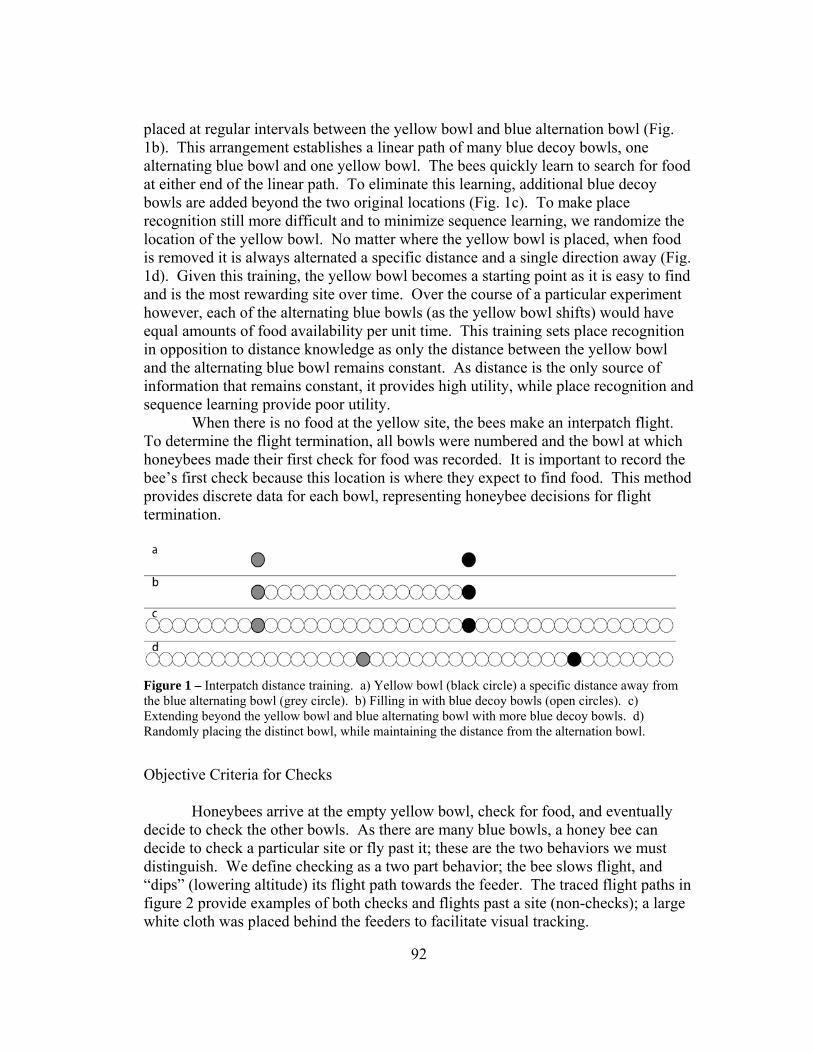
placed at regular intervals between the yellow bowl and blue alternation bowl (Fig. 1b). This arrangement establishes a linear path of many blue decoy bowls, one alternating blue bowl and one yellow bowl. The bees quickly learn to search for food at either end of the linear path. To eliminate this learning, additional blue decoy bowls are added beyond the two original locations (Fig. 1c). To make place recognition still more difficult and to minimize sequence learning, we randomize the location of the yellow bowl. No matter where the yellow bowl is placed, when food is removed it is always alternated a specific distance and a single direction away (Fig. 1d). Given this training, the yellow bowl becomes a starting point as it is easy to find and is the most rewarding site over time. Over the course of a particular experiment however, each of the alternating blue bowls (as the yellow bowl shifts) would have equal amounts of food availability per unit time. This training sets place recognition in opposition to distance knowledge as only the distance between the yellow bowl and the alternating blue bowl remains constant. As distance is the only source of information that remains constant, it provides high utility, while place recognition and sequence learning provide poor utility. When there is no food at the yellow site, the bees make an interpatch flight. To determine the flight termination, all bowls were numbered and the bowl at which honeybees made their first check for food was recorded. It is important to record the bee’s first check because this location is where they expect to find food. This method provides discrete data for each bowl, representing honeybee decisions for flight termination.

Figure 1 – Interpatch distance training. a) Yellow bowl (black circle) a specific distance away from the blue alternating bowl (grey circle). b) Filling in with blue decoy bowls (open circles). c) Extending beyond the yellow bowl and blue alternating bowl with more blue decoy bowls. d) Randomly placing the distinct bowl, while maintaining the distance from the alternation bowl.

Objective Criteria for Checks Honeybees arrive at the empty yellow bowl, check for food, and eventually decide to check the other bowls. As there are many blue bowls, a honey bee can decide to check a particular site or fly past it; these are the two behaviors we must distinguish. We define checking as a two part behavior; the bee slows flight, and “dips” (lowering altitude) its flight path towards the feeder. The traced flight paths in figure 2 provide examples of both checks and flights past a site (non-checks); a large white cloth was placed behind the feeders to facilitate visual tracking.

92

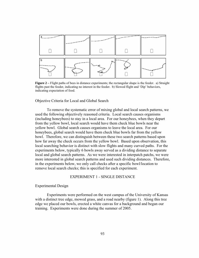
Figure 2 – Flight paths of bees in distance experiments; the rectangular shape is the feeder. a) Straight flights past the feeder, indicating no interest in the feeder. b) Slowed flight and ‘Dip’ behaviors, indicating expectation of food.

Objective Criteria for Local and Global Search To remove the systematic error of mixing global and local search patterns, we used the following objectively reasoned criteria. Local search causes organisms (including honeybees) to stay in a local area. For our honeybees, when they depart from the yellow bowl, local search would have them check blue bowls near the yellow bowl. Global search causes organisms to leave the local area. For our honeybees, global search would have them check blue bowls far from the yellow bowl. Therefore, we can distinguish between these two search patterns based upon how far away the check occurs from the yellow bowl. Based upon observation, this local searching behavior is distinct with slow flights and many curved paths. For the experiments below, typically 6 bowls away served as a dividing distance to separate local and global search patterns. As we were interested in interpatch patchs, we were more interested in global search patterns and used such dividing distances. Therefore, in the experiments below, we only call checks after a specific bowl/location to remove local search checks; this is specified for each experiment.

EXPERIMENT 1 - SINGLE DISTANCE

Experimental Design Experiments were performed on the west campus of the University of Kansas with a distinct tree edge, mowed grass, and a road nearby (figure 1). Along this tree edge we placed our bowls, erected a white canvas for a background and began our training. Experiments were done during the summer of 2005.

93

Figure 1 – a) Sketch of the experimental area. Light shading indicates forest, dark shading indicates asphalt, the line indicates a road and the white area is mowed grass. Here, the dots represent the location of the 40 feeders.

To test whether honeybees know the distance between two patches (interpatch distance knowledge) we used the above experimental design with 40 bowls, spaced 0.75m apart; the bowls were numbered 1-40. This large number prevents honeybees from using counting measures as recently described by (Dacke and Srinivasan 2008). We chose 8 possible locations for the yellow bowl to be placed; these were location 5, 7, 9, 11, 13, 15, 17, and 19. The alternation bowl was always 12 meters (16 bowls) away making the alternation locations 21, 23, 25, 27, 29, 31, 33, and 35, respectively. We then randomized the sequence at which we place the yellow bowl. A typical sequence of food availability would be something like the following (bold indicates the yellow bowl): 5-21-15-31-9-25-7-23-19-35-11-27-17-33-13-29. Once all eight locations of the yellow bowl were used, we randomized the sequence for the next yellow bowl locations. Honeybees were trained for four weeks before testing. During testing we recorded honeybee checks for one minute after removing food from the yellow bowl, leaving no food available at any of the bowls. After testing, food was placed at the correct alternation location and training resumed. Checks were only counted if they were 6 or more bowls from the yellow bowl to remove local searching bees from the analysis. Honeybees were tested for two weeks. Results Table 1 shows the statistical values of honeybee checking, indicating the location at which they expect to find food. We performed t-tests to test whether the honeybees were checking at the expected location. We conclude that the honeybees were not checking at the exact expected location, nor were they checking all feeders

94

equally (random). We also conclude that honeybees are not making random checks (p < 0.001, test not shown). We can also see that honeybees were not just choosing the closest alternation location 21 (p < 0.001, test also not shown). Table 1 – Statistical measures of checks for each test position. The p-values indicate a t-test for the expected value.

Yellow Bowl n mean ± SE expected p

5 82 20.8 ± 0.2 21 0.494

7 98 22.4 ± 0.2 23 0.029

9 98 22.5 ± 0.2 25 <0.001

11 98 24.0 ± 0.2 27 <0.001

13 82 25.3 ± 0.3 29 <0.001

15 66 28.3 ± 0.3 31 <0.001

17 98 30.3 ± 0.2 33 <0.001

19 98 30.6 ± 0.1 35 <0.001

To discover the honeybee’s decision making strategy, we had to equalize the different test positions. To do so, we subtracted the expected bowl number from each of the observed checks, thus making correct decisions have zero values, too short distances have negative values, and too long distances have positive values. We then superimpose each test position on top of eachother to obtain a histogram of the honeybee checking, relative to the expected value (0 error). This superimposition effectively measures their error and is shown in Figure 2. Here, honeybees made checks with an average error of -2.40 ± 0.1 (mean ± SE) with a noticeable absence of checks after the expected location. While this quantified information of checks is useful for understanding the decision making of honeybees, we also observed some qualitative behaviors after the honeybees had made their initial checks. The stereotypical behavior would be for honeybees to make their initial check and then continue checking in the same direction. We therefore conclude that in order to make such decisions, honeybees know the approximate distance to the correct location, but decide to check cautiously a few feeders before.

95

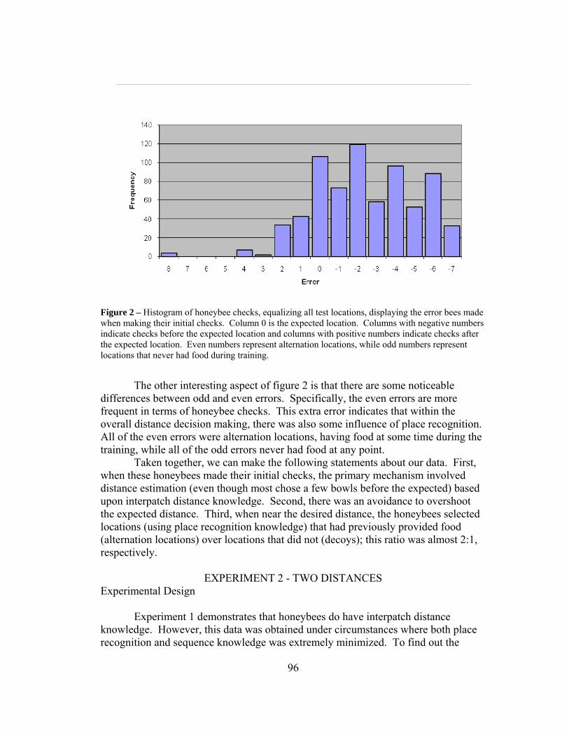
Figure 2 – Histogram of honeybee checks, equalizing all test locations, displaying the error bees made when making their initial checks. Column 0 is the expected location. Columns with negative numbers indicate checks before the expected location and columns with positive numbers indicate checks after the expected location. Even numbers represent alternation locations, while odd numbers represent locations that never had food during training.

The other interesting aspect of figure 2 is that there are some noticeable differences between odd and even errors. Specifically, the even errors are more frequent in terms of honeybee checks. This extra error indicates that within the overall distance decision making, there was also some influence of place recognition. All of the even errors were alternation locations, having food at some time during the training, while all of the odd errors never had food at any point.

Taken together, we can make the following statements about our data. First, when these honeybees made their initial checks, the primary mechanism involved distance estimation (even though most chose a few bowls before the expected) based upon interpatch distance knowledge. Second, there was an avoidance to overshoot the expected distance. Third, when near the desired distance, the honeybees selected locations (using place recognition knowledge) that had previously provided food (alternation locations) over locations that did not (decoys); this ratio was almost 2:1, respectively.

EXPERIMENT 2 - TWO DISTANCES Experimental Design

Experiment 1 demonstrates that honeybees do have interpatch distance knowledge. However, this data was obtained under circumstances where both place recognition and sequence knowledge was extremely minimized. To find out the

96

relative influence these cognitive tools have, we had to allow for the possibilities of the others. We chose the same experimental location as mentioned above (figure 1) and used the same amount of bowls (40), spaced0.75m; these experiments were performed during the summer of 2006. To test whether honeybees can keep track of two locations at different distances, but in the same direction, we trained the bees to the following conditions. The yellow bowl was placed at location 1 and had two blue alternation bowls at locations 17 and 27; the rest of the locations were filled by blue decoy bowls. During the morning (0800 to 1030 hours), food availability was alternated between the yellow bowl and location 27 and in the afternoon (1230 to 1530 hours) between the yellow bowl and location 17. At all other times, the food was located at the yellow bowl (location 1). Honeybees were trained for a week. During testing the yellow bowl was moved from location 1 to location 6, then food was removed from all sites. Thus, if honeybees were using distance knowledge as a priority, they would be expected to check five bowls (3.75m) after the expected locations (locations 22 and 32, instead of the 17 and 27). Twenty checks were recorded and then training was resumed. Checks were only counted after honeybees passed location 11. Honeybees were tested for a week. Results Figure 3 displays the recorded checks for the morning and afternoon treatments. The data here was bimodal, requiring us to analyze each possible location differently. The two most important locations for honeybees to check were locations 17 and 27. Therefore, we looked at the amounts of checks at these exact locations and a few bowls before and after. Area one (A1) included checks from bowls 12-21 and area two (A2) included checks from bowls 22-31. In the morning, when food was removed from the yellow bowl, the average for A1 was 17.12 ± 0.3; in the afternoon the average for A2 was 24.85 ± 0.3(mean ± SE). The expected values, based upon the yellow bowl shift were 22 and 32, respectively. On sample t-tests reveal that in neither case were they checking the shifted locations of 22 and 32; p < 0.0000001 in both cases. Instead, the honeybees were checking near the place where they had previously been; the two modes exactly match the locations of 17 and 27. We conclude that honeybees were choosing place recognition cues over distance cues as the primary determinant of decision making.

To discover the secondary influences on decision making we used two-sample t-tests to look for slighter preferences in decision making. When holding the location constant (morning A1 vs. afternoon A1 and morning A2 vs. afternoon A2) both tests were highly significantly different from eachother (p < 0.001) with a preference for the correct choice (afternoon A1 and morning A2) indicated by higher numbers of checks. Thus, honeybees were able to choose correctly based upon time. When holding the time constant (morning A1 vs. morning A2 and afternoon A1 vs. afternoon A2) both tests were highly significantly different from eachother (p < 0.001) with a preference for the correct choice (morning A2 and afternoon A1)

97

indicated by having a higher number of checks. Thus, honeybees were able to choose correctly between two recognized places, based upon distance (e.g. flying over A1 to A2).

We also noticed a tertiary influence in the following way. When we compare the two incorrect choices (morning A1 vs. afternoon A2) and the two correct choices (morning A2 vs. Afternoon A1), both tests are marginally significantly different (p-values of 0.035 and 0.053, respectively) with a slight preference for A1. This data shows that there was a small preference for honeybees to choose the closer location, when all other variables are constant. We have three major conclusions based upon experiment 2. First, honeybees used place recognition to terminate their departure directions more than any other cue. The two alternation locations were well known. Second, there was an effect of time and distance on the departure decisions, each of which allowed the bees to make informed decisions about where to go. Third, given these two potential locations, there was little motivation to simply choose the closest location.

Figure 3 – Histogram of honeybee checks in the morning and afternoon times. In the morning, food alternated to location 27, in the afternoon, 27.

EXPERIMENT 3 - THREE DISTANCES

Experimental Design We chose the same experimental location as mentioned above (figure 1) and used the same amount of bowls (40), spaced 0.75m from each other; these experiments were also performed during the summer of 2006. To test whether honeybees can keep track of three locations at different distances, but in the same direction, we trained the bees to the following conditions. The yellow bowl was placed at location 4 and had three alternation bowls at locations 15, 25, and 35; the rest of the locations were filled by decoy bowls. During the morning (0800 to 1000

98

hours), food availability was alternated between the yellow bowl and location 25, at noon (1130 to 1330 hours) between the yellow bowl and location 15, and in the afternoon (1500 to 1700 hours) between the yellow bowl and location 35. At all other times, the food was located at the yellow bowl (location 1). Honeybees were trained for four weeks. During testing the yellow bowl stayed at location 4 and food was removed from all sites. Test were performed in two ways, initial and subsequent. Initial tests are tests at the time when honeybees have no previous experience with the upcoming treatment, while subsequent tests are taken after the honeybees had experience with the treatment a few times on that day. This analysis effectively allows us to distinguish differences in long-term memory and short-term memory; further detail is outlined in (need references). Twenty checks were recorded and then training was resumed. Checks were only counted after honeybees passed location 10. Honeybees were tested for 3 weeks. Results The data here was tri-modal, requiring us to analyze each possible location differently. The three most important locations were 15, 25, and 35. Therefore, we looked at the amounts of checks at these locations and a few bowls before and after. We labeled these areas S1 (bowls 11-20), S2 (21-30) and S3 (31-40) and expected the most checks at S2 in the morning, S1 at noon, and S3 in the afternoon.

Figure 4 displays the recorded initial checks for the morning, noon, and afternoon treatments. The initial checks give us insight into the long-term memory of the honeybee and specifically, the information stored in their place maps.

Figure 4 – Histogram of honeybee checks in the morning and afternoon times. In the morning, food alternated to location 27, in the afternoon, 27.

We performed two sample t-tests to determine the similarities between S1, S2,

and S3 in the morning, noon, and afternoon; this can be found in table 2. Here, we

99

find no evidence the honeybees are using the time of day as a predictive stimulus for the correct distance to food, based upon their long-term memory. Table 2 – Two sample t-tests for each area (S1, S2, and S3) with for each pair of testing times for initial tests (N = noon, M = morning, and A = Afternoon). The p-values are representative of 8 degrees of freedom or more. The major point to notice is that there is a relatively high amount of similarity (compared to Table 3) in these initial trials, indicating that honeybees made similar decisions during the morning, noon, and afternoon times.

S1 p S2 p S3 p

N vs. M 0.885 N vs. M 0.463 N vs. M 0.071

N vs. A 0.130 N vs. A 0.067 N vs. A 0.643

M vs. A 0.014 M vs. A 0.071 M vs. A 0.250

Figure 5 displays the recorded subsequent checks for the morning, noon, and afternoon treatments. The subsequent checks give us insight into the short-term memory of the honeybee, not expected to be information stored in the place map.

Figure 5 – Histogram of honeybee checks in the morning and afternoon times. In the morning, food alternated to location 27, in the afternoon, 27.

We performed two sample t-tests to determine the similarities between S1, S2, and S3 in the morning, noon, and afternoon; this can be found in table 3. Here, we show that honeybees are indeed capable of using the time of day as a predictive stimulus to choose the correct distance among three feeding locations, once they have had some experience at that location during that day.

100

Table 3 – Two sample t-tests for each area (S1, S2, and S3) with for each pair of testing times for subsequent tests (N = noon, M = morning, and A = Afternoon). The p-values are representative of 8 degrees of freedom or more. The major point to notice is that there is massive difference between times of the day when the food was available at a specific location (shaded below) and in all cases, this is the result of more checks during those times at the specific location. This data indicates that during subsequent trials, honeybees made extremely different decisions and that these decisions are biased towards the location of the food.

S1 p S2 p S3 p

N vs. M < 0.0001 N vs. M < 0.0001 N vs. M 0.141

N vs. A < 0.0001 N vs. A 0.063 N vs. A < 0.0001

M vs. A 0.591 M vs. A < 0.0001 M vs. A < 0.0001

Figure 6 displays the recorded checks for all treatments (morning, noon, and afternoon, as well as initial and subsequent) lumped together. Lumped data allows us to understand the general tendencies of the honeybees, independent of the time, or expected distance to travel.

Figure 6 – Histogram of honeybee all checks independent of the time of day. Here, we see that all alternation locations are well (15, 25, and 35) and that there is a preference for checking the closest location.

We performed an analysis of variance on these to discover the relationship

among these three areas. Here, F = 49.63 and p < 0.000001, where S1 > S2 > S3. This data indicates that honeybees chose the closest feeder (in area S1) more frequently than the other two and that after S1, S2 was the most frequently chosen. Therefore, honeybees have an underlying choice for the closest feeders, independent of the time of day and expected distance to travel.

We have three major conclusions based upon experiment 3. First, given the complexity of this interpatch foraging paradigm, the honeybees were preferentially checking the closest feeder. Second, the place map of honeybees, in this context,

101

does not use the time of day as a predictive stimulus for interpatch foraging distance. Third, the bees are more than capable of choosing the proper location (distance knowledge and place recognition cues as well) once they know where food is.

DISCUSSION

Interpatch Distance Knowledge

First and foremost, honeybees know interpatch distance knowledge; however, there is an interaction with the other cues available to them. Experiment 1 demonstrates that given eight potential alternation locations (that were randomly fed) honeybees can use their interpatch distance knowledge to guide their foraging decisions, likely increasing foraging efficiency. Experiment 2 demonstrates that given two potential alternation locations that were fed in a temporally predictive manner, the honeybees chose to use place recognition knowledge over distance knowledge, while showing a small preference for the closer location. Experiment 3 demonstrates that given three potential alternation locations that were fed in a temporally predictive manner, they again used place recognition over distance knowledge. However, in this context they showed a greater preference for the closer location, an intermediate preference for the middle location, and the least preference for the farthest location (figure 6). In addition, when using their long-term memory, they seemingly used little to no distance knowledge when checking for food. When using their short-term memory, they were quite precise in their checking, choosing the appropriate location while avoiding the closer feeder in the morning and afternoon; this indicates the use of both distance and place recognition knowledge.

Taken together, we make the following statements about the knowledge base of honeybees, with respect to interpatch distance knowledge. Honeybees will choose place recognition knowledge over distance knowledge, whenever place knowledge has utility, although both are used. When honeybees are using such place recognition knowledge, their checks are quite precise (modes of the histograms at the location of alternation). When they use distance knowledge, they choose to check a few locations before the location of alternation and continue checking further.

Lastly, closer examination of the data (not presented here) shows that a small percentage of the honeybees could have been using distance knowledge primarily and in essence, solving our problem. However, we did not track individuals, choosing first to understand the general trends first, before searching for inter-individual differences. ADDITIONS TO THE PLACE MAP The experiments presented here are useful in updating our knowledge about the mind of honeybees and we purposely avoid calling our conclusions evidence for cognitive maps or labeling them “map-like”. Instead, we add them to our objectively defined place map (self reference – Chapter 1); this is a simple and consensus concept

102

derived from the shared components of all cognitive map theories. The new additions to the place map, based upon the information presented here, are two-fold.

First, honeybee place maps include interpatch distance knowledge that can be used to make efficient foraging decisions. This knowledge seems to be used secondarily to place recognition knowledge, but can be used if place recognition is unknown or provides little utility. Second, with this newly discovered interpatch distance knowledge, we can describe the information of the place map as vector encoded by uniting the interpatch direction knowledge (self reference – Chapters 2, 3, 4, and 5), interpatch distance knowledge (shown here), and the vector components of the dance communications. All currently described paths (outward, homeward, and interpatch) are stored in the mind of the honeybee as vector quantities. The Mind of the Honeybee Honeybee cognition, and honeybee biology in general, has gained in popularity in recent years. With these new techniques, we now have the ability to investigate the mind of the honeybee in greater detail. With these honeybees, we are able to extend such high level cognition past previously expected taxonomic bounds. When humans close their eyes and imagine space, we get some form of a geometric understanding of our world. When a honeybee is foraging and trying its best to make efficient decisions, it may have some form of this geometric understanding, although probably lower in resolution. In essence, not only is the newly described cognitive ability far greater than what we previously imagined, but we should expect it to be even more complex because of their foraging efficiency. We have the adequate techniques to study these abilities in detail, manipulate the sources of information, and truly discover how good these honeybees are.

103

Chapter 7

Investigating Shortcut Making The Shortcut When Tolman (1948) first described the mammalian cognitive map, the ability to make novel shortcuts was a defining characteristic. However, what was not required was complete vector knowledge, which honeybees have. An experiment performed by Karl von Frisch and his collaborators (Von Frisch 1967) mirrored Tolman’s experiment greatly. Both of these experiments forced the organisms to perform a dog-leg (L-shaped) path and unite the beginning and ends with a shortcut. Here, the shortcut path in von Frisch’s experiment was actually expressed in the dance language, indicating that their cognitive computations were quite abstract as the actual shortcut path could not be flown. At this time, there was little talk discussion of cognitive maps in honeybees. Given the evidence from Karl von Frisch, his data fully satisfies the criteria of Tolman’s cognitive map and is enough to establish cognitive maps in honeybees. History, however, seems to have an unfortunate story to tell; this is the “controversy of the cognitive map”.

When Gould (1986) first proposed that cognitive maps were present in honeybees, he too used the concept of the novel shortcut. Similar to Tolman’s experiment, the honeybees performed quite similarly to the mice. Gould used active displacements however, changing much of the details, but the defining characteristic (the shortcut) was met. This data represented yet another example of cognitive mapping, based upon the original description. Unfortunately, what followed proved to be less useful than expected. Various investigators, not willing to prescribe a high level of cognition in the honeybee, sought to disprove Gould’s cognitive map and not necessarily Tolman’s. Various extra-original criteria were added to the concept of the cognitive map, many to seemingly exclude honeybees from the discussion of cognitive mapping. This discrepancy expanded exponentially as the vertebrate research moved forward with leaps and bounds after the discoveries of place, grid, head direction, and other spatial information cells. Still other groups, especially with pigeons, observed these birds being able to navigate from positions they had never been and at far greater distances than honeybees can manage (Papi and Wallraff 1992). The theoretical question was then asked many times, “What is a cognitive map.” (Mackintosh 2002). There are two answers to this question. The first, gives precedent to the historical progression and is simply, “The cognitive map is what Tolman defined it to be.” Many people are not happy with this answer, thus striving to get further description and redefine the cognitive map themselves, leading to the second answer. The second answer to this question gives precedent to the subsequent progression since Tolman’s initial description and is simply “The cognitive maps of different species show enormous amounts of variation.” The theory of evolution would predict this variation as it is unlikely that two species (especially

104

taxonomically diverse groups like mammals and insects) need exactly the same cognitive map. As investigators defined their own versions of the cognitive map in their particular species, they maintained the same term for different concepts. Thus, the term cognitive map could mean many things. Even within the honeybee literature cognitive map theories are diverse enough to the point of nullifying the concept. This nullification occurs when a single experiment (Gould 1986) can verify one version of the cognitive map (Tolman 1948) and simultaneously dismiss another version of the cognitive map (Menzel et al. 1990). The only result of this conceptual disparity is confusion and leads to unnecessary controversy. The Place Map We have created a new concept, capable of incorporating Tolman’s original definition, as well as any other version of the cognitive map. It is evolutionarily sound, relying on the simplest elements of cognition that can be expanded upon. It is also discipline non-specific as we found the consensus elements of all cognitive maps, again, that can be expanded upon. The place map is the foundation, and the specific cognitive skills of honeybees make the honeybee place map. We acknowledge both von Frisch’s and Gould’s shortcut demonstrations as an addition to the honeybee place map; shortcuts can be produced by the process of path integration, as originally defined (Jander 1957). Displacement vs. No Displacement Gould and many later experimenters used displacement to force honeybees to do specific tasks. Here, we argue that the function of the honeybee place map is not realized when active displacement is used. In reality, honeybees are not likely to be displaced into unfamiliar environments. There should be a more ecologically relevant reason to know and be able to fly shortcuts. Honeybees are extremely efficient foragers, their cognition is more likely to be a result of maximizing this efficiency, not fighting against wind. Ecological Utility for Motivation

Every plant ecologist learns about the temporal and spatial properties of flowers. In addition, the concepts of species richness and species evenness are fundamental in understanding the variability in plant distributions. This variation is what the honeybee has to try to understand when trying to maximize the amount of resource they can get per unit time. The major flowering traits that we want to focus on now are the temporal availability of nectar how this variability relates to the spatial distribution of plants. Temporal availability of nectar is important because for any given area of flowers, nectar is potentially available at different times of the day (this variation can be species specific or even population specific). With respect to this situation, every single time honeybees fly out to a location, there are two possibilities:

105

either the flowers have nectar or not. It is in this situation that the motivation to produce shortcuts is relatively high.

Imagine if honeybees are foraging 1000 meters away from the colony, then all of a sudden the flowers stop producing nectar. All the honeybees could either give up and go home and thereby waste 2000 meters worth of flight energy (outward and homing paths) or choose to make an informed decision by making an interpatch flight to another location that contained resources. In order to do so, the honeybees would need to know something about the location of both places, relative to eachother. With our previous research showing that all paths of the place map are encoded with vector information (distance and direction) it is easy to now say that honeybees have this type of knowledge. The real trick is to make them do it, to motivate the behavior.

Below we present a new method used to motivate such shortcut interpatch paths, based upon the ecological principles of flower characteristics. In essence, we needed to demonstrate that interpatch paths between secondary hubs are path integratable, just like the homing paths from the colony.

Study 7 - “Generation of Novel Shortcut Interpatch Paths Using Realistic, Ecologically Based Motivations in the Honeybee (Apis mellifera)”

Producing Shortcuts We were able to induce the motivation for honeybees to make shortcut interpatch paths in by providing ecologically relevant training. Our ability to measure this shortcut ability was rather limited and further modifications of this general training should prove to make it easier. Once it becomes easier to measure, we can analyze the decision making with respect to interpatch shortcut paths as we have done before with interpatch direction and distance. Where to Go Next In all our experiences with honeybee foraging, we noticed some behaviors that intrigued us and led us to believe that there was still more to be understood. In essence, it appeared that we weren’t challenging the bees. These tasks we asked honeybees to perform were primarily based upon investigating and challenging the theories made by humans with poor assumptions, not the cognitive abilities of honeybees. Granted, some honeybees appeared to struggle while others appeared to understand completely. The next test then would be to challenge the honeybees by increasing the complexity of experiments, to investigate their learning and understanding capabilities in a few new dimensions.

106

Generation of Novel Interpatch Shortcut Paths Using Realistic,

Ecologically Based Motivations in the Honeybee (Apis mellifera)

Danny Najera, Liz Munz, Natalie Peters, Rudolf Jander

INTRODUCTION

The ability of organisms to make novel shortcuts was the original criteria of Tolman (1948). Whenever novel shortcuts are brought up in the honeybee literature, the experiments by (Gould 1986, Dyer 1991, Menzel et al. 1990, Menzel et al. 2005) come to mind. Every single one of these uses artificial displacement of honeybees from one location to another. The ecological relevance of such a displacement has been subject to question many times. The most consist explanation to this ecological relevance has been that of wind, blowing honeybees off course to another location. Once at this new location, they could calculate a novel shortcut to get to where they needed to go. We contend that there is a better reason for ability and seek to find realistic, ecologically based motivations that could select for the cognitive ability to make novel shortcuts.

TESTING FOR NOVEL ROUTES – NEW METHODOLOGY

Experimental Design All other previous attempts regarding novel routes in honeybees involve the spatial displacement of individual bees from one location to the other. This displacement can affect the motivational state of a honeybee and alter its immediate behavior. We chose not to spatially displace the honeybees, but instead displace the resources that they are interested in with respect to time; the procedure is as follows.

We placed a hive in a gap of a row of dense trees and bushes. The next morning honeybees were trained to a location on the south side of the tree line; afterwards, food was removed. The same afternoon, we trained them to the north side of the tree line; afterwards, food was removed. Once these honeybees knew both locations, we trained them in the following way. For location one (morning), the honeybees were fed from 8:00 a.m. to 11:30 a.m. Food was then removed from all locations for two hours (11:30 a.m. to 1:30 p.m.). From 1:30 p.m. to 5:00 p.m. the honeybees were fed at location two (afternoon). Both location 1 and location 2 were fed equal concentrations with similar scents. Location 1 was 140m from the hive, location 2 was 125 m from the hive and location 1 was 50m from location 2; this is shown in figure 1. This training was continued for at least one week before testing. We wanted to know if honeybees knew how to fly from location 1 to location 2 without training and without artificial displacement. In this case it would be a novel shortcut, based upon the fact that they would have never had motivation to do so

107

previously. To generate this motivation, we needed to overlap the food availability of these locations to mimic the variation in flowering times in the natural context. Testing consisted of allowing food availability to continue at location 1 until 1:30 p.m (instead of terminating at 11:30 a.m.). At 1:30 p.m. on a testing day, food would be removed from all locations and individual honeybees would be tracked to see if they flew from location 1 to location 2. Instead of having a 2 hour period of no food (from training) food would be available at location 2; this provides the necessary motivation for making an interpatch shortcut.

Because we did not spatially displace any of these bees, we gain an interesting perspective of natural foraging behavior that has previously eluded many investigators. A significant drawback to this situation is that once the temporal overlap in food availability has occurred and a test has been run, the same hive cannot be tested again as the shortcut would no longer be novel. Therefore, each hive was tested once and each test took a single day before a new hive was brought in. Experiments were performed on the west campus of the University of Kansas with distinct tree edges, in a hay field (figure 1). Experiments were performed during the summers of 2006, 2007, and 2008.

Figure 1 – Sketch of the experimental area with the relevant treelines found in a hayfield (not drawn to scale). The distance between 1 and 2 is 50m, between 1 and H is 140m, and between 2 and H is 125m.

Tracking Individuals For our specific data measurements, we relied on a simple time calculation. Here, we painted individual honeybees using Testor ® enamel based paints and recorded the times they departed location 1 and the times they arrived at location 2 and computed the difference between the two. Departure times from location one were recorded once the honeybee had left the feeder and was visually determined to not be circling the feeder (global search patterns). Often, this determination would be 10 or 20 meters from the feeder and a few seconds after leaving the feeder itself. This delay creates a systematic error that biases our recorded times towards quicker flights.

108

To account for this, we added 2 seconds to all of our departure times. Arrival times were much more precise as the honeybees were landing at the feeder and being recorded much quicker. By computing the difference between these two recorded times, we have the amount of time that it took for the individual honeybee to fly from table 1 to table two, independent of the path that was flown. Results

Over the course of three summers, we tested 8 hives according to the above design, each with some minor modifications. Out of these 8 hives, we individually marked 288 honeybees. Of these less than 40 % (112) were given recordings for both location 1 departures and location 2 arrivals. For those that did have both recordings, we selected the 19 fastest honeybees and show these in figure 2.

Figure 2 – A linear plot of recorded times for individual honeybees making the flight from location 1 to location 2. The gray box indicates the individuals that are considered to have made novel shortcuts.

We then calculated the theoretical amount of time it would take for unloaded honeybees flying 7.5 m/s (Wenner 1963) to make the straight line path from location 1 to location 2; this time is 6.67s. In addition, we calculated the time it would take for honeybees flying back to the colony from location 1, then to location 2; this time is 35.32s. Because we did not take into account the actual flight paths, we must be conservative in our conclusions. Therefore, any individual honeybee that makes the trip (from location 1 to location 2) in the interval of 6.67s (perfect shortcut) and 35.32s - 3s will be considered a novel shortcut for a total of 10; we subtracted 3 seconds to be sure the honeybees did not actually reach the colony, before arriving at location 2. Of these shortcuts, those closest to 6.67s (8s, 9s, and 12s) must indicate direct novel shortcuts (3 individuals).

DISCUSSION Ecological Relevance Honeybees are capable of making these novel shortcuts given ecologically relevant motivations. We know that flower nectar production varies tremendously within and between species. When resources run out, honeybees are faced with a decision to return home empty handed or to check other profitable areas. In a natural

109

setting, it is easy to imagine many flowers and that when one species stops producing nectar, another will be. Therefore, the efficiency of the colony can be greatly impacted by the ability to switch from one flower patch to another. In most natural contexts, either during nectar flows or not, this switch will occur every single day (potentially multiple times a day) for an extended time over the course of the year. This variability is an ecological situation that is quite common and the results we have shown allow us to make a few predictions.

We should expect that some of the honeybees that we painted went to check other potential resources as well. We should expect that each individual has its own subset of information about the resources around the colony, even given only one week to develop it. It may even be that given enough honeybees, all possible resource locations are checked every time a resource runs out. This strategy would effectively disperse the foraging cohort from one location to many. With the communicative abilities of honeybees, all it takes is a single individual to find the right place to be and re-establish a strong cohort on the profitable patch.

From another perspective, we know that honeybees search for possible resource locations from the hive. Based upon previous research (self reference – Chapter 5) we should expect that honeybees search for food from locations other than hives, specifically from secondary hubs (familiar locations other than the hive). We fully believe that if a honeybee can search from the colony, they can search from a secondary hub. Theoretically, this type of novel route shown here should be absolutely expected. Measuring Novel Shortcuts

Based on our measurements, only a total of 3 honeybees made direct shortcuts (from location 1 to location 2), 10 made any general shortcuts (from location 1 to location 2). These proportions are 2.7% and 8.9%, respectively, of the total number of individuals that had both measurements (112). Without doubt, these data represent a low proportion in terms of recognizing this behavior and there are two things that we can do to likely improve this proportion: include path analysis, change the relative concentrations and locations to maximize the number of bees performing such paths. With path analysis, easily provided harmonic radar at these distances (Riley et al. 1996), a greater number of these general shortcuts may become direct shortcuts. In addition, many of the honeybees that did not satisfy our time increment as shortcuts could likely be considered as shortcuts (our low percentages would only go up). Regardless, our aim was not to measure the frequency at which shortcuts occur, but instead to determine if such novel shortcuts were possible based upon ecologically relevant motivations; this has been demonstrated. For manipulations of the relative concentrations of sugar, we could make location 2 more or less profitable and potentially with odors different than location 1. For manipulations of locations, we could make the distance from location 1 to location 2 closer or farther, and increase the distance at which both location 1 and 2 are from the hive. We expect that continued work with this experimental design will

110

prove fruitful so that we can more closely explore the decision making for novel shortcuts.

Experimental Design Considerations

The largest drawback to our experimental design is that this test can only be

performed a single time with the current techniques. Once these times are overlapped and honeybees fly the novel routes, the route is no longer novel and a new group of honeybees (a new hive) will be needed. Without a good sized apiary, the number of tests one can perform is extremely limited (we tested 8 hives over three years).

Theoretical Relevance To put things in perspective, let us consider other paths that we know of that can be considered shortcuts and when these shortcuts can be considered novel. There are at least three major paths that that we can sometimes consider as shortcuts: homing paths, interpatch paths, and direction encoding waggle paths of waggle dances.

For homing paths, when an individual forages on multiple flowers over a widely distributed area, these homing paths are unlikely to be in the exact opposite direction as the original outward path, making it a shortcut. Whenever this homing shortcut is performed from a location that has not been visited before, it is a novel shortcut; honeybees are well known for this behavior. It has been shown, in this context, that path integration can generate these novel shortcuts (Von Frisch 1967), but given the opportunity, honeybees can use previously known points of reference to guide their movements (Von Frisch 1967, Cartwright and Collett 1982).

For interpatch paths, all of these are shortcuts, linking two locations together, and independent of the hive (point of origin) itself. Honeybees have been well documented to visit multiple patches of flowers, based upon the contents they obtain and bring back to their colony. The first time the honeybee flies this path it must be novel. The research presented here demonstrates that honeybees do, in fact, make such novel interpatch shortcut paths. We are unaware at this point of the informational cues that they use to do so, but expect them to be similar to the previously quantified interpatch cues (self reference – Chapters 2, 3, 4, and 5). Lastly, Karl Von Frisch demonstrated the most theoretically interesting novel shortcut described to date (1967, pp.173-183). Here, during the waggle dances, honeybees were able to produce a cognitive shortcut path (direction specific) even though they were unable to fly the path itself. This novel shortcut is purely cognitive because it had never been flown, nor would ever be flown. Such a novel shortcut can be derived by path integration machinery involving vector quantities of the known paths. Shortcuts are not at all unfamiliar to this organism. Novel shortcuts are less common, but still widely dispersed in different contexts. Tolman (1948) used the ability to make novel shortcuts as a criterion for the cognitive map. Since then, the

111

definition of a cognitive map has changed drastically (Gallistel 1989, Mackintosh 2002). Yet, all cognitive map descriptions used for honeybees (as well as Tolman’s original description) are less complex than the level at which the honeybee is operating. Unfortunately, it seems as if such previous theories are more concerned with the perceived ability at which an insect should be able to operate, rather than the level of complexity at which its livelihood depends on (flowering plants). Based upon recent experiments (self reference – Chapters 2, 3, 4, and 5) such novel interpatch shortcut paths should be expected. The ability of these honeybees to interpret information, compute efficient strategies, and make effective decisions is uncanny. The Mind of the Honeybee

There are multiple reasons why these honeybees are so good at what they do. One of these reasons is the dance language, but we now know that it is so much more than that. In the tiny exoskeleton head of theirs is an insect equivalent of a geographic plant ecologist. Their cognitive abilities match the ecological difficulties that face them. Individuals find resources by searching, once found, they dance. Sometimes they search their knowledge based upon prior experience to generate novel shortcuts. This intelligence is how they make their living, with great individual and collective intelligence.

112

Chapter 8

Challenging the Honeybee

Complexity – Is it a game? When people ask me what I do as a graduate student, I often say the following about honeybees and my work:

I am interested in comparative cognition. Specifically, the cognition involved with spatial understanding and decision making. My job has been to discover the full extent of honeybee intelligence. To this point, I have failed.

The honeybees, more often than not, have easily handled our experiments. Based upon observation, these honeybees seem to increase in number as complexity of the foraging goes up. For instance, while at a specific concentration, fewer honeybees will be present at a single stationary feeder when compared to our complex foraging situation. When we switch from a complex training situation to a single stationary feeder (if we are going to be absent for a few days) relatively few bees show up. The easiest way I have begun to understand this observation is through a human understanding and human examples. When people do puzzles or various challenging tasks of their minds, they don’t do simple arithmetic and they don’t do simple jigsaw puzzles. The mind of the human likes to be challenged, to the point that more challenge often gives us pleasure. I see this trait in honeybees as well, and so, I thought to challenge them past all expectations, and they performed brilliantly. The following experiment had quite a consistent cohort, potentially because of how fun the complexity was. Simultaneous Manipulation of Information We chose decision making as our topic to make more complex. In this case, we decided to make a single secondary hub with three auxiliary locations. To add complexity, we made one of these auxiliary feeders in the third dimension (or Z-axis). In addition, we used one predictive stimulus (time) and two linked stimulus (lemon and vanilla odors) for the honeybees to keep track of in order to make well informed decisions. This resulted in decision making that included four locations to decide among from the secondary hub (home and the three auxiliary locations), in all three dimensions of space, based upon three stimuli (time and two odors), and two motivational states (hungry and satiated). To make it even more difficult, we made the stimuli contingent upon each other so that they had to track both stimuli simultaneously to make the most efficient decisions. This research is presented below, in a condensed format as it was designed to be published in a high-tier journal.

113

Study 8 - “Logic in Honeybees (Apis mellifera); Demonstration of conditional, syllogistic reasoning in the context of foraging.”

Six Dimensional Decision Making – Two Term Conditional Reasoning When surveying the literature of complex decision making, we found no honeybee and no non-human animal studies involving this complexity. By all measures, this experiment was designed to push the envelope of animal cognition and to challenge these honeybees. Within all the complexity, the simplest way to represent this complexity of decision making by honeybees is through a six-dimensional decision making process. The decisions they had to make involved the following: motivational state, odor, time of day and all three dimensions of space. Each of these must be considered for all of the proper decisions to be made. This decision making is more intriguing than the dances themselves, more intriguing than communication, and still, even to me, almost unbelievable. These results will force us to redefine our understanding of animal cognition.

114

Logic in Honeybees (Apis mellifera); Demonstration of Conditional, Syllogistic Reasoning in the Context of Foraging.

Katie Holzer, Danny A. Najera, Rudolf Jander

INTRODUCTION

How much intelligence can a honeybee possess? With such small brains and a nervous system organized so differently from ours, could they be performing similar functions such as logical reasoning? These are loaded and complex questions, but we can start to gain insight to the answers by analyzing the behavior of foraging honeybees, using the novel methods described by (self reference – Chapter 1 and Chapter 5).

We use the term logic here in reference to deductive reasoning and Aristotle’s logical progression of the conditional syllogism. Such a syllogism contains three parts: a premise, an antecedent, and a consequent. Aristotle’s classic example is as follows:

The premise is: All men are mortal. The antecedent is: Socrates is a man. The consequent is: Socrates is mortal. In this form of deductive reasoning, the antecedent and the consequent are

similar to an “If..., then...” statement, made relevant only in light of the premise. In terms of honeybees, this logic can be tested by training them to a specific pattern (establishing the premise) such that if a certain set of conditions is present (antecedent), then the honeybees should fly a specific distance and direction to find resources (consequent). Being able to make these kind of decisions would likely make resource gathering more efficient, especially when computing shortcuts (self reference) and therefore increase the likelihood of the survival of the colony, and in turn, the species. We would expect to discover this complex reasoning being used at secondary hubs (self reference – Chapters 5 and 7). Indeed, it may even be that deductive reasoning and logic have evolved convergently in humans and honeybees.

To test this possibility, we enabled interpatch foraging with honeybees, training and testing them under a set of complex, but consistent conditions to see if they could learn and reason through the complexity. Based upon the previous research, honeybees have been shown to use complex decision making in the following ways: (self reference – Chapter 5). While these experiments were conducted separately, we mean to step up the complexity by combining them into one experiment. Here, we focused on the direction component and not the distance component of decision making.

METHODS

115

Study Area and Training

We trained and tested foraging honeybees on the West Campus of the University of Kansas in June and July of 2005. Using the standard incremental method of training (von Frisch, 1967), we trained honeybees to forage at a central feeding table X, 222m from hive (Figure 1). Using the interpatch method of training (self reference – Chapter 1) we set up three auxiliary locations (A, B, and C). Auxiliary locations A and B were 10m away from X and in the horizontal plane (90° CCW and 180° from the direction home, respectively) while location C was at the top of a 5m flagpole directly above X. Figure 2 shows the layout of these three auxiliary locations.

Figure 1 - Sketch of study area. H is hive, X is the testing site. The light grey areas are deciduous forests. The small dark rectangle is a building and the large black rectangle is an asphalt football field. The lines are gravel roads. X is 222m from H along the bees’ flight path (not as the crow flies).

116

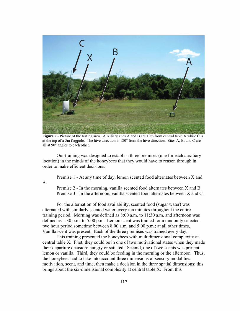
Figure 2 - Picture of the testing area. Auxiliary sites A and B are 10m from central table X while C is at the top of a 5m flagpole. The hive direction is 180° from the hive direction. Sites A, B, and C are all at 90° angles to each other.

Our training was designed to establish three premises (one for each auxiliary location) in the minds of the honeybees that they would have to reason through in order to make efficient decisions.

Premise 1 - At any time of day, lemon scented food alternates between X and

A. Premise 2 - In the morning, vanilla scented food alternates between X and B. Premise 3 - In the afternoon, vanilla scented food alternates between X and C. For the alternation of food availability, scented food (sugar water) was

alternated with similarly scented water every ten minutes throughout the entire training period. Morning was defined as 8:00 a.m. to 11:30 a.m. and afternoon was defined as 1:30 p.m. to 5:00 p.m. Lemon scent was trained for a randomly selected two hour period sometime between 8:00 a.m. and 5:00 p.m.; at all other times, Vanilla scent was present. Each of the three premises was trained every day. This training presented the honeybees with multidimensional complexity at central table X. First, they could be in one of two motivational states when they made their departure decision: hungry or satiated. Second, one of two scents was present: lemon or vanilla. Third, they could be feeding in the morning or the afternoon. Thus, the honeybees had to take into account three dimensions of sensory modalities: motivation, scent, and time, then make a decision in the three spatial dimensions; this brings about the six-dimensional complexity at central table X. From this

117

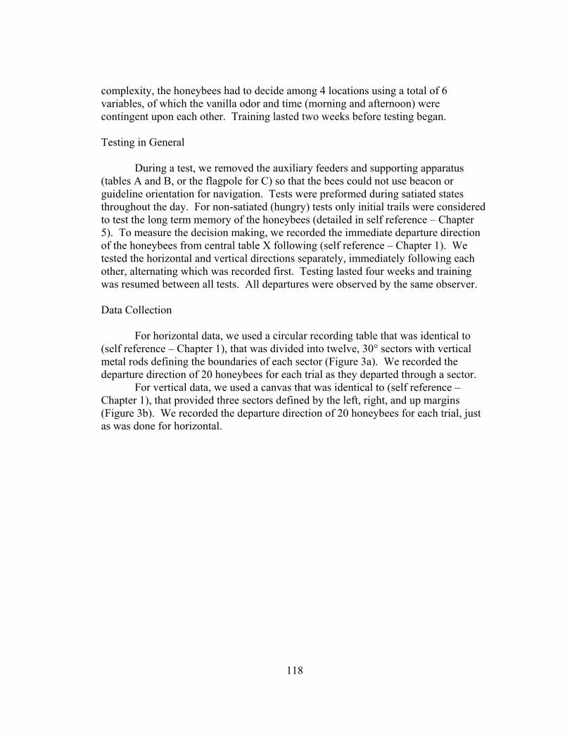
complexity, the honeybees had to decide among 4 locations using a total of 6 variables, of which the vanilla odor and time (morning and afternoon) were contingent upon each other. Training lasted two weeks before testing began. Testing in General During a test, we removed the auxiliary feeders and supporting apparatus (tables A and B, or the flagpole for C) so that the bees could not use beacon or guideline orientation for navigation. Tests were preformed during satiated states throughout the day. For non-satiated (hungry) tests only initial trails were considered to test the long term memory of the honeybees (detailed in self reference – Chapter 5). To measure the decision making, we recorded the immediate departure direction of the honeybees from central table X following (self reference – Chapter 1). We tested the horizontal and vertical directions separately, immediately following each other, alternating which was recorded first. Testing lasted four weeks and training was resumed between all tests. All departures were observed by the same observer. Data Collection For horizontal data, we used a circular recording table that was identical to (self reference – Chapter 1), that was divided into twelve, 30° sectors with vertical metal rods defining the boundaries of each sector (Figure 3a). We recorded the departure direction of 20 honeybees for each trial as they departed through a sector. For vertical data, we used a canvas that was identical to (self reference – Chapter 1), that provided three sectors defined by the left, right, and up margins (Figure 3b). We recorded the departure direction of 20 honeybees for each trial, just as was done for horizontal.

118

Figure 3 - a) Circular measuring table for horizontal data collection. Central table X was divided into 12 sectors of 30° each. The table has a diameter of 1m. Bees departed from the feeder in the center and their departure sector was recorded as data. b) White canvas next to central table X in the 90° direction. This canvas was used for measuring vertical departure directions with sectors of left, up, and right. Because it was so close to the table, bees were not likely to depart directly into it, thus preferentially biasing the data in opposite direction.

RESULTS

For the horizontal data we calculated the mean vector direction (VD) and vector length (VL) for each trial. For the vertical data we measured the number of departures through each sector and report here the up data. For satiated honeybees, n = 24, and for each non-satiated antecedent, n = 18. Satiated Honeybees We tested honeybees while food was present at table X; these honeybees were allowed to feed until satiation. For the horizontal data, we expected the honeybees to depart towards the Hive located at 0° or 360°; we recorded a VD of 306° ± 19.00 and a VL of 0.61 ± 0.03 (mean ± stdev). The resulting histogram is reported in Figure 4b. For the vertical data, we did not expect the honeybees to depart towards location C; we recorded 2.33 ± 1.82 (mean ± stdev) departures through the up margin per trial (data not shown). Hungry (Non-Satiatied) Honeybees

If Lemon, Then Table A (Antecedent and Consequent 1)

119

We tested honeybees when the following situation occurred at table X: no

food and lemon scent. For the horizontal data, we expected the honeybees to depart towards table A at 270°; we recorded a VD of 260° ± 12.6° and a VL of 0.68 ± 0.08 (mean ± stdev). The resulting histogram is reported in Figure 4c with the mode in the expected sector 9. For the vertical data, we did not expect the honeybees to depart towards location C; we recorded 5.56 ± 3.76 (mean ± stdev) departures through the up margin per trial (figure 5).

If Vanilla and Morning, Then Table B (Antecedent and Consequent 2)

We tested honeybees when the following situation occurred at table X: no food, vanilla scent, during the morning. For the horizontal data, we expected the honeybees to depart towards table B at 180°; we recorded a VD of 205° ± 11.02° and a VL of 0.60 ± 0.15 (mean ± stdev). The resulting histogram is reported in Figure 4d with the mode in the expected sector 6. For the vertical data, we did not expect the honeybees to depart towards location C; we recorded 4.67 ± 2.00 (mean ± stdev) departures through the up margin per trial (figure 5).

If Vanilla and Afternoon, Then Location C (Antecedent and Consequent 3) We tested honeybees when the following situation occurred at table X: no food, vanilla scent, during the afternoon. We expected the honeybees to depart towards table C and have no preference in departure in the horizontal direction (random horizontal departures) as table C was directly above central table X; we recorded a VD 274 ± 33.59 and a VL of 0.33 ± 0.13 (mean ± stdev). The resulting histogram is reported in Figure 4e. For the vertical data, we expected the honeybees to depart towards location C; we recorded 11.00 ± 2.49 (mean ± stdev) departures through the up margin per trial (figure 5).

Figure 4 – Horizontal departure directions of honeybees (lumped data) from the center table X. a) Schematic of the relationship of locations to eachother. A and B are in the horizontal plane while C is directly above the center table X. b) Satiated departures, after feeding. c) Hungry departures, lemon scented water (no food). d) Hungry departures, vanilla scented water during the morning. of satiated and bees. e) Hungry departures, vanilla scented water during the afternoon. The numbers at the end

120

of the columns represent how many bees departed through that sector throughout all of the trials. The modes of lemon and morning vanilla are in the expected directions. The data for afternoon vanilla are random if the canvas (90°) is taken into account. Each of these decisions is in line with logical reasoning.

0

2

4

6

8

10

12

14

Ave

rage

Up

Vertical Departures

Lemon Morning AfternoonVanilla Vanilla

Figure 5 - Histogram of the number of honeybees departing through the up sector (from central table X) of our horizontal departure data collection setup. The error bars indicate the standard error of the mean. Significantly more honeybees departed through the up sector when they discovered vanilla scented water (no food) in the afternoon, when compared to the other treatments (lemon scented water and vanilla scented water in the morning (p < 0.00002). There was no significant difference in the up departures of lemon and morning vanilla (p = 0.384).

STATISTICAL TESTS

Between Groups

The trail-specific data were our entry points for analysis to ensure statistical independence. Because the trial statistics were sufficiently clumped, linear statistics were applied to the test various null hypotheses. We follow the statistical testing of (self reference – Chapter 1).

First, we ran t-tests for the vector direction (VD) of each pair of the three antecedents. There was a significant difference between the mean VD of lemon and vanilla-morning as well as between vanilla-morning and vanilla-afternoon (p <

121

0.000001 for both). There was no difference between lemon and vanilla-afternoon (p = 0.107).

Second, we ran t-tests for the vector length (VL) of each pair of the three antecedents. There was no significant difference between the VL of lemon and vanilla-morning (p = 0.088). There was a significant difference between lemon and vanilla-afternoon as well as between vanilla-morning and vanilla-afternoon (p < 0.000001 and p = 0.000002, respectively).

Third, we ran t-tests for the vertical up departures for each pair of the three antecedents. There was no significant difference between lemon and vanilla-morning (p = 0.384). There was a significant difference between lemon and vanilla-afternoon as well as vanilla-morning and vanilla-afternoon (p = 0.000018 and p < 0.000001, respectively). In these situations, vanilla-afternoon had the highest amount of up departures. The Effect of the Canvas

By looking at the data in Figure 4, you can see that the departures through sectors 2, 3, and 4 are considerably lower than other sectors. This lack of departures is due to the canvas erected for the vertical data recording, causing the data to be biased in the direction towards location A (270°). Because of this bias, one-sample t-tests show significant deviations from our expected directions. These deviations are non-informative and we focus on the major trends when analyzing our data, not the fine detail deviations. Here, the modes of the data are clearly representative of the decision making in these honeybees.

CONCLUSIONS

Given the complexity in our experimental design, we have a simple conclusion to make. The honeybees chose efficiently and within our expectations. Given the antecedents of lemon scented water, vanilla scented water in the morning, and vanilla scented water in the afternoon, they correctly reasoned out the proper consequents: food should be at locations A, B, and C respectively. With respect to the horizontal plane, we can make the following statements. When deciding to depart to location A, honeybees made departures (VD) towards location A with high values of VL. When deciding to depart to location B, honeybees made departures (VD) towards location B with similarly high values of VL. When deciding to depart to location C, honeybees have no distinct preference for horizontal departures (except to avoid the canvas) and should not as location C is not located horizontally; this was reflected in low values of VL. With respect to the vertical axis, we can make the following statements. When deciding to depart to location A the amount of up departures is relatively low. When deciding to depart to location B, the amount of up departures is similarly low. When deciding to depart to location C, the amount of up departures is extremely significantly higher.

122

Taken together (horizontal and vertical), there are only two explanations as to how these recorded observations could come about. Either a) the honeybees possess the previously described reasoning capabilities or b) different groups of honeybees are making only one decision; this presents itself as a systematic error in our testing. Fortunately, we can distinguish between these two possibilities in the following way. Systematic Error Testing

It is possible that there were different groups honeybees during the different testing times. If different groups were present, an individual bee would only need to know the location of one auxiliary site and would not need to make a complex decision. To test for this systematic error, we performed a pseudo mark-recapture study, following (self reference Chapter 5), where we marked 500 individuals one day at location A (with lemon scent). The next day we counted the number of total honeybeesbees at the feeder as well as the number of marked bees every 30 minutes for the entire 9 hours; this includes counts for all antecedents. There was no significant difference between any of the proportions of marked honeybees to unmarked honeybees (p > 0.05) with an overall mean of 0.5654 ± 0.01 (mean ± SE). This proportion shows that the same honeybees are present during all conditions. When tracking a single honeybee we would find it at all feeding locations, as well as making all decisions at the central table X. This testing effectively removes the possibility that different groups were making only one decision.

Additional Data – Short-term and Long-term Memory We also did subsequent testing in addition to the initial tests mentioned above; this follows (self reference – Chapter 5). We found no difference between the two, indicating that all of this information is stored in their long term memory, allowing them to solve this problem without any previous experience during that day. This data indicates that within their cognitive repertoire they are linking different concepts to their place map and can use these links to reason out proper decisions.

DISCUSSION Honeybees are capable of deductive logical reasoning, based upon the classical definitions of the conditional syllogism. This demonstrated logical reasoning is capable of handling 6-dimensional complexity to choose among 4 possible outcomes (Figure 6). From an information theory perspective, this decision involves a minimum of three bits of information to be used for an immediate decision; also in Figure 6. Given the complexity of the honeybee place map (self reference – Chapter 1) we must now acknowledge that the place map (and all derivations of the cognitive map) is just the tip of the ice berg. Honeybees are capable of networking their spatio-temporal place map with different sensory modalities, in the same reference frame; space, time, and odor, are brought together.

123

We predict that honeybees are able to network more than just space time and odor, but this is the first study to do so. One can only imagine what else exists within the cognitive repertoire of honeybees that is still left undiscovered. Yet, the strength of these results is not necessarily to demonstrate the capabilities of honeybees, but instead to compare this discovery to other species, specifically our own.

Figure 6 – The simplest representation of the how honeybees need to make the efficient decisions observed. The 6-dimensional complexity comes from the motivational state, odor, time, and 3 dimensions in space. Notice that food availability is not predictable for locations B and C unless both the odor and the time are considered simultaneously. The information coding is the simplest binary representation of the information with respect to the decision making.

Possessing logic is something that humans often reserve for themselves, with Aristotle himself believing that it was a fundamentally unique quality of humans, distinguishing them from non-human animals. Given the research presented above, we can no longer accept this assumption as 100% true. Even though the overall brain organization between honeybees and humans is drastically different, the ability to make logical decisions has evolved convergently. This level of complexity is also undocumented as we were unable to find any non-human animal study involving decision making with this many parameters. In addition, the fact that this complexity has been discovered in an insect forces us to fundamentally reconsider our preconceived notions of cognition and what a relatively small (there are smaller) nervous system can do.

We must open our minds to progress forward and seriously reconsider our preconceived notions of animal cognition. We have absolutely no knowledge at this point that would allow us to predict how such complex cognition exists in the honeybee brain. Something about our understanding of intelligence, brains, and the interaction between the two is fundamentally flawed. Studies similar to ours should be attempted in a wide range of organisms help the process of redefining our thoughts about cognition and intelligence so that we can progress. In animal behavior, we have already been blown away by these honeybees and their dances, have always been fond of them, but until now, had no idea just how amazing they truly are.

124

Acknowledgements We would like to thank Dr. Orley “Chip” Taylor for the use of his bees as well as Erin McCullough and Patricia Van Meter for their previous studies that led to ours. Funding provided to Katie Holzer by the National Science Foundation Research Experience for Undergraduates Program.

125

Chapter 9

Summary of Research A New Perspective The majority of the research presented in this manuscript is a result of four new approaches to understanding honeybee knowledge. First, we focused on the interpatch path; previous research focused on outward and homing paths. Second, we gave our honeybees massive amounts of familiarity with extended training; previous research focused on displacing honeybees and the lack of familiarity. Third, we built a new recording device to measure honeybee departures that focused on a single location in space where we could define all sources of information; previous research used compasses and vanishing bearings. And fourth, we analyzed immediate departures of honeybees; previous research allowed the honeybees ample time to make more than one decision.

Functionally, my duty was to take these new approaches and discover the utility within them. From this realized utility, we have been able to investigate the cognition of honeybees with unprecedented accuracy and precision. We have been able to answer questions that were previously unable to be asked. We now have the tools to understand the relative influence that each stimulus has on decision making and analyze the context specificity of this influence. With these new approaches and the extreme motivation for foraging in honeybees, we have the best tools to analyze the mind of any non-human animal (arguably). With these tools we have discovered a complex mind, breaking down the preconceived expectations of animal cognition. The Recent Failure of the Cognitive Map For roughly two decades, research focused on whether or not honeybees have cognitive maps. This research has lead to massive controversy and little progression towards the understanding of honeybee cognition. We strongly urge all researchers to abandon the concept of the cognitive map (at least honeybee researchers) for the following reasons. 1) There is no consistent definition of the cognitive map. 2) The variation of cognitive map definitions creates contradictions within the concept itself. 3) The cognitive map is an understatement for honeybees, with little ability to describe gradation that is expected when comparing species. It is unfortunate that Edward Tolman’s original cognitive map concept (1948) has come to such a pass. The Utility of the Place Map To recover our objectivity, we have created a new concept for the complexity of high level spatial understanding; this is the place map. This place map is a simple and consensus concept derived from the shared properties of cognitive map definitions and is much more robust to differences among species as each species is

126

expected to have species specific additions to this basic place map. In fact, the evolution of such place maps may turn out to be much more interesting than just the place map of the honeybee; this perspective is impossible for the cognitive map at present. Below, we describe the honeybee place map by defining the general place map and listing a few of the additions provided by the original research of Karl Von Frisch (1967) and all of the additions based upon our research shown here. The Place Map and Additions

- The place map is defined as the mental representation and recall of two or more places, linked with topomotor route knowledge or spatial vector knowledge. The recall of known places is facilitated by place specific cues. Topomotor route knowledge is represented by the sensorimotor instructions used to navigate from one known place to another. We state that such place maps are latently learned through exploration.

- We used the classical experiments of Karl von Frisch (1967) to demonstrate the data based examples of these criteria.

- Three additions to the honeybee place map were added based upon other information from Karl von Frisch (1967); these are marked “Von Frisch”. The rest of the additions listed here are from our research presented here. Specifically, we can now say the following about the honeybee place map:

o It is three dimensional – Von Frisch o It maps space and time in the same reference frame – Von Frisch o It is path-integrateable (hive to patch) – Von Frisch o It contains vector encoded information (interpatch and not) – Chapters

2, 3, and 6 o It can be used to create sequence specific paths – Chapter 4 o Includes primary and secondary hubs (useful for branching decision

making) – Chapter 5 o Uses predictive and linked stimuli to make branching decisions away

from the hive – Chapter 5 o It is path-integrateable (patch to patch) – Chapter 7 o It links other modalities together in the same reference frame,

specifically color and odor – Chapter 8 Impact on Previous Theory The research presented here, in summary, has progressed previous theory in the following ways, by chapter. Chapter 1

127

- We created a new concept for understanding the cognitive abilities of foraging honeybees; this is the place map.

- We introduced our new methodology, interpatch training techniques, experimental designs, data collection devices, verifying their effectiveness.

- Provided objective criteria by which we can distinguish specific behaviors for data collection

Chapter 2

- We began investigating landmark theory with respect to beacon and compass orientation.

- We were able to demonstrate that both could be used by honeybees and that neither dominated

- We were able to demonstrate our methodological power by accurately separating various stimuli from one another (this would be used time and time again).

- We also demonstrated some flexibility of our new methods in terms of modeling, quadrant analysis and sector comparisons.

Chapter 3

- We investigated landmark theory by checking for terrestrial and celestial compass use, in combination and in isolation of each other.

- We were able to demonstrate that honeybees need no terrestrial cues to guide their interpatch departure direction and that celestial cues were sufficient.

- We were able to show that different cues had different statistical values of VL, providing future investigation about the relative magnitude of use and reliability of specific stimuli.

Chapter 4 - We began investigating route theory with respect to sequence learning. - We were able to demonstrate that honeybees can learn three (qualitatively

different) experimentally defined sequences based upon 3 or 4 feeding locations.

- Based upon small, unexpected deviations in our data, we were able to get a glimpse of the effects of context on decision making. Specifically, we noticed that hives pull departures towards their directions and that there are some effects of tree lines on the decision making of honeybees.

- We introduced a pseudo-mark-recapture technique used to remove systematic errors based upon potential subgroups of honeybees within the larger population.

Chapter 5 - We investigated route theory by showing that branching decisions can be

made and that sequences were not sufficient in explaining the observable foraging behavior of honeybees.

128

- We introduced the concepts of primary hub, secondary hub, auxiliary locations, predictive stimuli and linked stimuli, along with definitions.

- We were able to demonstrate specific qualities of primary hubs and specific types of stimuli (color, odor, time of day) that could be predictive or linked at secondary hubs

- We were able to show that secondary hubs can be familiar, non-familiar, have food, or never have food.

- We introduced the techniques to differentiate between short and long-term memory based upon their experience prior to testing.

Chapter 6 - We presented the new methodology to investigate interpatch distance

knowledge and a few tools that can be used to subtract utility of place recognition and sequence learning.

- Provided objective criteria by which we can distinguish specific behaviors for data collection.

- We demonstrated that honeybees possess interpatch distance knowledge and we began to define the hierarchical preference of cues when honeybees decide to terminate flight, while demonstrating deficiencies in the linkage of concepts to interpatch distance knowledge.

- We were able to show an example of massive differences between short-term memory and long-term memory, based uponthe methods from chapter 5.

- Effectively demonstrated that honeybees possess complete vector knowledge of interpatch paths, making the entire place map vector based.

Chapter 7 - We began investigating the shortcut making (the original criterion of cognitive

maps) in honeybees. - We demonstrated ecologically relevant contexts in which shortcut making is

highly beneficial to honeybees. - We described all other known shortcuts, to emphasize that shortcuts are

relatively familiar to honeybees, and that interpatch foraging paths are shortcuts.

Chapter 8 - We began to push the limits of not only honeybee cognition, but non-human

cognition in general. - We created the most complex (that we could find) experimental decision

making study to date involving 6 dimensional complexity and 4 different decisions. Within this complexity, we made two stimuli contingent upon each other.

129

- We demonstrated, step by step, the similarity of the honeybee decision making to the classical syllogistic reasoning of Aristotle.

- We integrated both horizontal and vertical decision making with a two part testing procedure to analyze the three dimensional decision making.

- We calculated the number of bits of information necessary to make such a decision.

Pushing the Limits Even with our new place map concept in hand, along with all of the additions, we have not accounted for the complexity discovered in the cognitive repertoire of these honeybees. Instead we have tapped into a much larger unity of cognitive systems, linking multiple concepts as well as different sensory modalities; this complex cognition must be in place to describe the logical reasoning we discovered in Chapter 8. At this beginning state, we are not quite certain what to label everything, but the term cognitive nexus, or reasoning nexus, may apply. More research is needed before this labeling is done, however. The Beloved Honeybee - Revisited Humans and honeybees share many unexpected similarities, of which we now know involves some aspects of logic. Recently, the general public has discovered how important honeybees are to agricultural production, causing many people to care for the honeybees; this is still motivated by self interest of course. More so now than ever, we can use them as an education tool, to allow the general public to witness another great mind from the biodiversity around them. While many of the charismatic fauna have little relevance to the survival of humans (pandas, whales, koalas, etc.) the honeybee is linked to the human society at present. Because of this interaction, the honeybee may serve as an ambassador to the human race, ushering in a new understanding of the necessity of ecosystems and biodiversity, redefining the level of respect and admiration we give to other living organisms, and providing yet another mind-blowing example of complexity from our beloved honeybee. The honeybee links human to plant, city dweller to farmer, and in my case, human-intellectual to honeybee-intellectuals.

I strongly believe that by showing the behavior of honeybees to people, we can change the behaviors of humans in a positive way. The human species is ready to be more responsible, the non-human organisms just need a spokesman (spokesbee if you wish); I believe this organism is our beloved honeybee.

130

Literature Cited Batschelet, E. (1981). "Circular Statistics in Biology." New York: Academic Press. Beekman, M., L. Doyen, et al. (2005). "Increase in dance imprecision with decreasing foraging distance in the honey bee Apis mellifera L. is partly explained by physical constraints." Journal of Comparative Physiology A: Neuroethology, Sensory, Neural, and Behavioral Physiology 191(12): 1107-1113. Benhamou, S. (1996). "No evidence for cognitive mapping in rats." Animal Behaviour 52: 201-212. Benhamou, S. and V. Seguinot (1995). "HOW TO FIND ONES WAY IN THE LABYRINTH OF PATH INTEGRATION MODELS." Journal of Theoretical Biology 174(4): 463-466. Bennett, A. T. D. (1996). "Do animals have cognitive maps?" Journal of Experimental Biology 199(1): 219-224. Bogdany, F. J., (1978) Linking learning signals in honeybee orientation. Behaviorial ecology sociobiology 3: 323-336 Brady, J. (1974) The physiology of insect circadian rhythms. Adv. Insect Physiol. 10:1-115. Cartwright, B.A., and Collett, T.S. (1982) How honey bees us landmarks to guide their return to a food source. Nature 295:560-564. Cartwright, B. A. and T. S. Collett (1983). "LANDMARK LEARNING IN BEES - EXPERIMENTS AND MODELS." Journal of Comparative Physiology 151(4): 521-543. Cartwright, B.A., and Collett, T.S. (1987) Landmark maps for honeybees. Biol. Cyber. 57:85-93. Cheng, K. (2000). "How honeybees find a place: Lessons from a simple mind." Animal Learning & Behavior 28(1): 1-15. Collett, T.S., and Cartwright, B.A. (1974) How lone bees use landmarks to guide their return to a food source. Nature 295:560-564. Collett, T. S. (1987). "INSECT MAPS." Trends in Neurosciences 10(4): 139-141. COMBA, L (1999) Patch use by bumblebees (hymenoptera apidae) temperature, wind, flower density and traplining. ETHOLOGY. ECOLOGY. EVOLUTION 11: 243-264 Dacke, M. Srinivasan, M. V. (2008) Evidence for counting in insects. Animal Cognition V. 11, I. 4, pps 683-689

131

Dyer, F. C. (1987). "Memory and sun compensation by honey bees." J. Comp. Physiol. A 160: 621. Dyer, F. C. (1991). "Bees acquire route-based memories but not cognitive maps in a familiar landscape." Anim. Behav. 41: 239. Dyer, F.C. (1993) How honey bees find familiar feeding sites after changing nesting sites with a swarm. Anim. Behav. 46:813-816. Dyer, F. C. 2000. Group movement and individual cognition: lessons form social insects. In: On the Move. How and Why Animals Travel in Groups (Ed. by S. Boinski & P. A. Garber), pp. 127-164. Chicago: University of Chicago Press. Dyer, A.G. Rosa, M.G.P., and Reser, D.H. (2008) Honeybees can recognize images of complex natural scenes for use as potential landmarks. J. Exp. Biol. 211 (April):1180-1186. Dyer, F. C. and J. L. Gould (1981). "Honey Bee Orientation: A Backup System for Cloudy Days." Science 214(4524): 1041-1042. Fisher, N. I. (1993). "Statistical Analysis of Circular Data." New York: Cambridge University Press. Foo, P., W. H. Warren, et al. (2005). "Do humans integrate routes into a cognitive map? Map- versus landmark-based navigation of novel shortcuts." Journal of Experimental Psychology-Learning Memory and Cognition 31(2): 195-215. Gallistel, C. R. (1989). "Animal Cognition: The Representation of Space, Time and Number." Annual Review of Psychology 40(1): 155-189. Giurfa, M. and E. A. Capaldi (1999). "Vectors, routes and maps: new discoveries about navigation in insects." Trends in Neurosciences 22(6): 237-242. Gould, J. L. (1976). "The dance-language controversy." Q. Rev. Biol. 51: 211. Gould, J. L. (1986). "The locale map of honey bees: do insects have cognitive maps?" Science v232: p861(3). Greggers, U., and Menzel, R. (1993) Memory dynamics and foraging strategies of honeybees. Behav. Ecol. Sociobiol. 32:17-29. Gross, H.J., Pahl, M., Zhu, H., Tautz, J., and Zhang, S. (2009) Number-based visual generalization in the honeybee. PLoS One 4(1):e4263. Healy, S., Hodgson, Z., and Braithwaite, V. (2003) Do animals use maps ? In: The Neurobiology of Spatial Behaviour. (Ed.: Jeffery, K.J.) Oxford University Press, New York, 104-118.

132

Jander, R. (1957) Die optische Richtungsorientierung der Roten Waldameise Formica rufa L. Z. vergl. Physiol. 40:162-238. Kirchner, W. H. and U. Braun (1994). "DANCING HONEY-BEES INDICATE THE LOCATION OF FOOD SOURCES USING PATH INTEGRATION RATHER THAN COGNITIVE MAPS." Animal Behaviour 48(6): 1437-1441. Mackintosh, N.J. (2002) Do not ask whether they have a cognitive map, but how they find their way about. Psicológica 23:165-185. Maurer, R. and V. Seguinot (1995). "WHAT IS MODELING FOR - A CRITICAL-REVIEW OF THE MODELS OF PATH INTEGRATION." Journal of Theoretical Biology 175(4): 457-475. Menzel, R., L. Chittka, et al. (1990). "DOMINANCE OF CELESTIAL CUES OVER LANDMARKS DISPROVES MAP-LIKE ORIENTATION IN HONEY-BEES." Zeitschrift Fur Naturforschung C-a Journal of Biosciences 45(6): 723-726. Menzel, R., U. Greggers, et al. (2005). "Honey Bees Navigate According to a Map-Like Spatial Memory." Proceedings of the National Academy of Sciences of the United States of America 102(8): 3040-3045. Menzel, R., Giurfa, M., Gerber, B., and Hellstern, F. (2001) Cognition in insects: The honeybee as a study case. In: Brain Evolution and Cognition. (Eds.: Roth, G., and Wullimann, M.F.) Wiley, New York, 333-366. Michener, C.D., and Grimaldi, D.A. (1988) The oldest fossil bee: apoid history, evolutionay stasis, and antiquity of social behavior. PNAS 85:6424-6426. Munz, T. (2005). "The Bee Battles: Karl von Frisch, Adrian Wenner and the Honey Bee Dance Language Controversy." Journal of the History of Biology 38(3): 535-570. Papi, F., and Wallraff, H.G. (1992) Birds. In: Animal Homing. (Ed.: Papi, F.) Chapman & Hall, New York, 263-319. Reinhard, J., Srinivasan, M., and Zhang, S. (2006) Complex memories in honeybees: Can there be more than two? J. Comp. Physiol. A 192:409-416. Renner, M. (1957) Neuere Versuche uber den Zeitsinn der Honigbiene. Z. vergl. Physiol. 40:85-118. Riley, J. R., U. Greggers, et al. (2005). "The flight paths of honeybees recruited by the waggle dance." Nature 435(7039): 205-207. Riley, J. R., A. D. Smith, et al. (1996). "Tracking bees with harmonic radar." Nature 379(6560): 29-30.

133

Robinson, G.E., and Dyer, F.C. (1993) Plasticity of spatial memory in honey bees: Reorientation following colony division. Anim. Behav. 56:311-320. Robinson, G.E., Fernald, R.D., and Clayton, D.F. (2008) Genes and social behavior. Science 322:896-900. Seeley, T.D. (1985) The information-center strategy of honeybee foraging. In: Experimental behavioral ecology and sociobiology. (Eds.: H”lldobler, B., and Lindauer, M.) Sinauer, Sunderland, 75-90. Seeley, T.D. (1996) The wisdom of the hive. The social physiology of honey bee colonies. Harvard Univ. Press, Cambridge MA. 295 pp. Shannon, C. E. (1948) A Mathematical Theory of Communication,'' Bell System Technical Journal, Vol. 27, pp. 379-423 and 623-656. Tanner, D. A., Visscher, K (2006) Do honey bees tune error in their dances in nectar-foraging and house-hunting? Behavioral ecology and sociobiology. V. 59, I. 4, pp. 571-576 Tolman, E. C. (1948). "COGNITIVE MAPS IN RATS AND MEN." Psychological Review 55(4): 189-208. Towne, W.F., and Moscrip, H. (2008) The connection between landscape and the solar ephemerids in honeybees. J. Exp. Biol. in Press:. Von Frisch, K (1914/15) der farbensinn und formensinn der bienen. Zool. Jahrbucher physiology. 35 1-1888 Von Frisch, K. (1967). "The Dance Language and Orientation of Bees." Cambridge Massachusettes: Harvard University Press. Von Frisch, K. and Lindauer, M. (1954) Himmel und Erde in Konkurrenz bei der Orientierung der Bienen. Naturwiss. 41:245-253. Vonfrisch, K. and R. Jander (1957). "UBER DEN SCHWANZELTANZ DER BIENEN." Zeitschrift Fur Vergleichende Physiologie 40(3): 239-263. Wahl, O. (1933) Beitrag zur Frage der biologischen Bedeutung des Zeitged„chtnisses der Bienen. Z. vergl. Physiol. 18:709-717. Wahl, O. (1932) Neue Untersuchungen űber das Zeitgedächtnis der Bienen. Z. vergl. Physiol. 16:529-589. Wehner, R. and R. Menzel (1990). "Do Insects Have Cognitive Maps?" Annual Review of Neuroscience 13(1): 403-414. Wehner, R. and S. Wehner (1990). "INSECT NAVIGATION - USE OF MAPS OR ARIADNES THREAD." Ethology Ecology & Evolution 2(1): 27-48.

134

135

Wenner, A. M. (1963). The flight speed of honeybees: a quantitative approach. J. Apic. Res. 2, 25-32 Zhang, S., Mizutani, A., and Srinivasan, M.V. (2000) Maze navigation by honeybees: learning path regularity. Learning and Memory 7:363-374.