redistribution from a lifetime · pdf fileredistribution from a lifetime perspective†...
TRANSCRIPT

Redistribution from a Lifetime Perspective
IFS Working Paper W15/27
Peter Levell Barra Roantree Jonathan Shaw

Redistribution from a Lifetime Perspective†
Peter Levell, Institute for Fiscal Studies and University College London
Barra Roantree, Institute for Fiscal Studies and University College London
Jonathan Shaw, Institute for Fiscal Studies and University College London
Abstract Most analysis of the effects of the tax and benefit system is based on snapshot information about a single cross-section of people. Such an approach gives only a partial picture because it cannot account for the fact that circumstances change over life. This paper investigates how our impression of redistribution undertaken by the tax and benefit system changes when viewed from a lifetime perspective. To do so, we simulate lifecycle data designed to be representative of the experiences of the baby-boom cohort, born 1945–54. We examine the properties of the current tax and benefit system as well as historical and hypothetical reforms from both a lifetime and a snapshot perspective. We find that much of what the tax and benefit system achieves is effectively to redistribute across periods of life and, as a result, it is much less effective at reducing lifetime inequality than inequality at a snapshot.
† The authors gratefully acknowledge a grant from the Nuffield Foundation (OPD/40976) and co-funding from
the European Research Council under the European Union's Seventh Framework Programme (FP/2007-2013) /
ERC Grant Agreement no. 269440 and the ESRC-funded Centre for the Microeconomic Analysis of Public
Policy at the Institute for Fiscal Studies (IFS) (RES-544-28-5001). The Nuffield Foundation is an endowed
charitable trust that aims to improve social well-being in the widest sense. It funds research and innovation in
education and social policy and also works to build capacity in education, science and social science research.
More information is available at http://www.nuffieldfoundation.org. We would also like to thank Stuart
Adam, James Browne, Carl Emmerson, Paul Johnson, Stephen Jenkins, Robert Joyce, Paolo Lucchino, Malcolm
Nicholls, Jonas Nystrom and Edward Zamboni for comments on earlier drafts of this paper. The English
Longitudinal Study of Ageing (ELSA) data were made available through the UK Data Archive (UKDA). ELSA was
developed by a team of researchers based at the National Centre for Social Research, University College
London and the IFS. The data were collected by the National Centre for Social Research. The funding is
provided by the National Institute of Aging in the United States, and a consortium of UK government
departments co-ordinated by the Office for National Statistics. Data from the Family Expenditure Survey,
Expenditure and Food Survey and Living Costs and Food Survey (LCFS) are Crown Copyright and reproduced
with the permission of the Controller of HMSO and the Queen’s Printer for Scotland. The British Household
Panel Survey (BHPS) is produced by the ESRC UK Longitudinal Studies Centre, together with the Institute for
Social and Economic Research at the University of Essex. Data for the BHPS were supplied by the UK Data
Service. The BHPS is also crown copyright material and reproduced with the permission of the Controller of
HMSO and the Queen’s Printer for Scotland. Any errors and omissions are the responsibility of the authors.
1
© Institute for Fiscal Studies
Executive summary
Most analysis looking at living standards and the redistribution achieved by the tax and benefit system has been based on snapshot information. This answers questions such as the following. How unequal is the distribution of current incomes? What is the impact of the personal tax and benefit system on current incomes? In this report, we analyse redistribution from a lifetime perspective, showing how this changes our view of inequality, what the impact the tax and benefit system is and what the implications are for policymaking. Background and methodology
The lifetime poor spend a considerable fraction of working life in paid work: individuals in the poorest decile (tenth of the population) of the lifetime net income distribution are employed for almost two-thirds of working life. Means-tested benefit entitlement is not restricted to individuals at the bottom of the lifetime distribution: on average, those in the richest decile of the lifetime income distribution spend almost one-fifth of their lifetime entitled to one of the main means-tested benefits. The poor are not always poor and (to a lesser extent) the rich are not always rich. For example, our simulations suggest that those in the bottom lifetime decile spend, on average, only 22% of life in the bottom snapshot decile. Those in the richest lifetime decile are in the top snapshot decile for an average of 35% of life. Redistribution achieved by the current tax and
benefit system
We model most personal taxes and benefits, but do not take into account ‘business taxes’ or the benefits from public service spending. Taking adult life as a whole, only 7% of individuals receive more in benefits than they pay in these taxes. This compares with 36% of individuals who receive more in benefits than they pay in these taxes in the cross-section. Some redistribution can be thought of as effectively being across periods of life, in the sense that the tax and benefit system gives at one age and takes at another, leaving lifetime incomes unchanged. Across all individuals, more than half of redistribution is of this ‘intrapersonal’ form. Income inequality is much lower from a lifetime perspective than a cross-sectional perspective: the Gini coefficient – a common measure of inequality – for gross income is 0.49 in the cross-section compared with 0.28 across the whole of adult life. This indicates that a lot of the inequality between

Redistribution from a lifetime perspective
2
individuals is temporary in nature, reflecting either the stage of life they are at or the transitory shocks they have experienced. The tax and benefit system is less effective at reducing inequality over the lifetime than in the cross-section. In the cross-section, it reduces the Gini coefficient by 31% but over the lifetime only by 15%. This reflects the fact that much of what the tax and benefit system does is intrapersonal redistribution. The effectiveness of the tax and benefit system at targeting lifetime outcomes is limited by the fact that most taxes and benefits are assessed over periods of a year or less, making it much easier to target outcomes over short horizons. Benefits are less effective at reducing lifetime inequality than they are cross-sectional inequality (a 14% fall compared with 31% fall) and direct taxes somewhat less effective (7% compared with 12%). Indirect taxes increase lifetime inequality by somewhat less than they increase cross-sectional inequality (7% compared with 13%): this is because those who temporarily have a low income often have high spending, and therefore a high indirect tax bill, relative to their low current income. State pensions are the most effective benefit at reducing inequality, but they are much more effective at reducing cross-sectional inequality (a 20% fall) than lifetime inequality (a 4% fall). This reflects the fact that pensioners tend to have low gross private incomes in the cross-section but not over the lifetime as the majority of people are pensioners at some point in their lives. Distributional effects of historical tax and benefit
reforms
Looking over the lifetime can alter our view of the progressivity of tax and benefit changes. Historical tax and benefit reforms over the last 40 years have affected lifetime inequality but not by as much as cross-sectional inequality. This could be by design but it is likely to reflect the fact that the tax liabilities and benefit entitlements are assessed on an annual or shorter-term basis. The Labour government’s expansion of in- and out-of-work benefits between 1999 and 2002 was well targeted towards the lowest three income deciles from a cross-sectional perspective. Over the lifetime, however, the reforms are much less targeted towards the bottom of the income distribution: the bottom six deciles all gain by at least 1% of net income. This is because many of the poorest individuals in the cross-section are not poor in all periods of life. The coalition’s tax and benefit reforms between 2010 and 2015 hit the cross-section poor most heavily (a loss of 7% in the bottom decile) but their impact extends over the whole income distribution from a lifetime perspective (all deciles lose by at least 1%).

Executive summary
3
The four-year freeze to working-age benefits and tax credit cuts announced in the July 2015 budget inflicts the greatest losses on individuals in the bottom three cross-sectional income deciles. Over the lifetime, the impact remains regressive but extends much further up the income distribution. For example, for the tax credit cuts, losses exceed 1% of net income in the bottom six deciles. Distributional effects of hypothetical tax and benefit
reforms
In the cross-section, increases in the main rate of VAT appear regressive, but not when looked at over the lifetime. This supports other analysis, which has found that increasing the main rate of VAT does not appear regressive when losses are expressed as a proportion of expenditure. Increases to VAT on zero- and reduced-rated goods are mildly regressive from a lifetime perspective. This is because the lifetime poor spend a greater share of their income on zero- and reduced-rated goods. However, it would be possible to design a reform package eliminating zero- and reduced-rating that pays for itself and is broadly distributionally neutral. In-work (i.e. work contingent) benefits are just as good at targeting the lifetime poor as out-of-work benefits, but do so without worsening work incentives by nearly so much. Changes to the higher rate of income tax do target the lifetime rich reasonably well, due to lower mobility at the top of the income distribution. Policy conclusions
Economic well-being should be evaluated over the lifetime and not just at a single point in time. The reason is simple: individuals typically live for many years, so it makes sense to measure outcomes over many years. Policies that alleviate short-run hardship may not target lifetime outcomes very well, and vice versa. To allow policy reforms to be assessed against their objectives, policymakers therefore need to be more explicit about what they are trying to achieve. For example, is a particular policy designed to alleviate short-run hardship or to reduce inequality in lifetime resources? A sharp distinction is often made in policy debates between working and non-working families. The reality is rather more complex, with most individuals experiencing substantial changes in their circumstances over the course of their lifetime. Policymakers looking to target the lifetime poor might favour doing so through in-work benefits because they are as progressive as increases in out-of-work benefits but have much less of a negative impact on work incentives.

Redistribution from a lifetime perspective
4
Policymakers looking to target the lifetime rich can do so reasonably well using the higher rate of income tax. This is because rich individuals tend to remain rich over prolonged periods of time. The current system of VAT distorts production and consumption choices towards zero- and reduced-rated goods and services instead of standard-rated ones. This is hard to justify on distributional grounds: removing zero and reduced rates is considerably less regressive from a lifetime perspective than in the cross-section, and it is possible to design a set of direct tax cuts and benefit increases that mean that the overall package is revenue neutral, broadly distributionally neutral and would avoid worsening work incentives. Because more than half of the redistribution that taxes and benefits achieve is intrapersonal, there may be efficiency gains from creating an explicit link between taxes paid at one point in life and benefits received at another. The reason for this is that taxes might be no longer perceived as pure (distortionary) taxes but at least partly as ‘social insurance’ contributions funding future benefits. However, the case is not clear-cut because it relies crucially on individuals recognising that contributions are not a tax but are a form of enforced saving that they value – and changing their behaviour as a result. None of analysis in this report suggests that the current tax and benefit system, assessed largely against contemporaneous circumstances, does especially well at redistributing resources towards the lifetime poor. Targeting lifetime redistribution more effectively may require new policy instruments that condition on longer-run circumstances.

5
© Institute for Fiscal Studies
1. Introduction
Individuals typically live for many years and their circumstances change substantially over the course of their lives. When evaluating their economic well-being, or the impacts on them of particular policies, it is therefore sensible to consider outcomes over their lifetime as a whole rather than just at a single point in time. Doing otherwise would be like determining the outcome of a football match based on what happens in a particular five-minute period of the match rather than over the full 90 minutes. That said, due to data limitations, most analysis of people’s living standards and the effects of the tax and benefit system is based on snapshot information about a single cross-section of people. For example, a standard measure of income inequality would look at the population at a point in time and measure the gap between those with the lower and higher current income.1 Similarly, a standard analysis of the distributional impact of a tax or benefit change would consider how it affects the distribution of current incomes. In this paper, we investigate how our impression of the redistribution achieved by the tax and benefit system changes when we take a lifetime perspective rather than the standard snapshot approach. The key thing that snapshot approaches cannot account for is that circumstances change over people’s life course, so some differences between people are temporary rather than permanent. For example, reforms that affect families with children will affect more people in a lifetime sense than in a snapshot sense, because some people who currently have no children will have children at another point in their lives. Also, reforms that affect those on high current incomes will, over a lifetime, have larger effects on the permanently rich than on those with temporarily high incomes. Using a snapshot, this distinction would be lost. In practice, the extent to which taking a lifetime perspective matters is an empirical question. Broadly, a snapshot measure will be relatively good at summarising what we want to know either if there is substantial immobility, so that current circumstances tell us a lot about lifetime circumstances; or if the current period is likely to be particularly important from a lifetime perspective. In earlier work (Roantree and Shaw, 2014), we investigated whether these reasons for caring about outcomes at a snapshot matter empirically. For the former (the degree of mobility), we showed that employment, earnings, family composition and disability all vary substantially across the lifecycle. For example, for earnings, we found that, while there is a high degree of ‘stickiness’ in the short term, there is a substantial amount of movement over longer horizons, 1 Examples include the annual Households Below Average Income (HBAI) publication from the Department for
Work and Pensions (DWP) (e.g. DWP, 2015) and IFS analysis based on the same underlying data (e.g. Belfield et al., 2015).

Redistribution from a lifetime perspective
6
particularly outside the top quintile of the earnings distribution. This suggests that, while snapshot outcomes might matter, it is important to analyse outcomes over the lifetime. With regard to the latter reason for caring about outcomes at a snapshot (the current period is particularly important), there are particular scenarios in which this might apply. In the case where income is the object of interest, these include borrowing constraints and uncertainty (which may make individuals unwilling to borrow because they cannot be sure of repaying loans in future). In these circumstances, it is not simply total lifetime income that matters, but also the timing of income: because individuals are unable to transfer income between periods of life by borrowing now and paying back later when income is higher, having a low income now may hurt welfare much more than having a low income in a later period once individuals have accumulated some savings and/or there is less uncertainty over future incomes. Are borrowing constraints and uncertainty empirically important? We tried to answer this in the work we cited above (Roantree and Shaw, 2014). For borrowing constraints, we found that many households are able to borrow, at least to some degree. Just under half of all households have some form of borrowing instrument and, focusing on households in their 20s (who may be most likely to be credit constrained because they have fewer assets such as housing that can be used as collateral), around 70% have non-mortgage debts. Thus, it seems that most households have at least some ability to borrow. Quantifying how important uncertainty is (e.g. in employment and earnings) is more difficult. The reason for this is that it requires data on subjective expectations about the future, little of which are available for the UK.2 Evidence does exist for other countries, however. For example, for the US, Manski and Straub (2000) present results for employment uncertainty and Dominitz (1998) gives evidence for earnings uncertainty. This work suggests that, while uncertainty does have an important role to play, individuals do nevertheless have a reasonable idea about their likely future employment and earnings, at least over relatively short horizons. So what do we conclude? Snapshot outcomes are likely to be important and informative, providing some indication of longer-run outcomes and (in the presence of borrowing constraints and uncertainty over future circumstances) highlighting individuals likely to be facing particular short-term hardship. However, they are unlikely to tell the whole story. For this, we additionally need to look at outcomes over the lifetime. Having established that lifetime outcomes matter, we now discuss the specific questions we attempt to answer from a lifetime perspective. We begin by analysing redistribution under the current (2015/16) tax and benefit system. We address the following. 2 While surveys such as the English Longitudinal Study of Ageing do include these data, this survey only covers
older people.
Introduction
7
How do taxes and benefits evolve across life? How do net contributions vary across individuals? How much redistribution is effectively across periods of life rather than across individuals? How effective is the tax and benefit system at reducing inequality? Which taxes and benefits are most effective at reducing inequality? We then go on to consider the distributional consequences of historical reforms to the tax and benefit system over the last 40 years. We investigate the following. How have reforms to the tax and benefit system over the last 40 years affected inequality? What were the distributional consequences of Labour’s expansion of in- and out-of-work benefits? What were the distributional consequences of the coalition’s tax and benefit reforms? What are the distributional effects of the benefit cuts in the July 2015 budget? Finally, we show how the distributional impact of some hypothetical reforms to the current tax and benefit system differs from a lifetime and a cross-sectional perspective. We ask the following questions. Where should resources be targeted to reduce inequality the most? How regressive are increases in VAT? What is the most effective way of redistributing resources to the lifetime poor: out-of-work benefits, in-work benefits or tax cuts? How well do tax changes target the lifetime rich? Answers to these questions matter because they have the potential to change our view of what impact the tax and benefit system has. For example, they will improve our understanding how taxes and benefits evolve across life, highlight the form that redistribution takes (across life or across individuals), demonstrate how effective redistribution is at reducing lifetime inequality and set out the distributional impact of various reforms from a lifetime perspective. This will naturally have implications for policy, as we seek to draw out. It is hard to undertake this analysis from a lifetime perspective because this requires data about full lifecycles. Unfortunately, no survey data set in the UK can provide a long enough time series, so instead we make use of simulation procedures. For concreteness, we focus on a single cohort, which we choose to be the baby-boom cohort. The advantage of this is that we have cross-sectional data covering most of the baby-boom cohort’s working life, which we can use to improve our simulations. The decision to focus on a single cohort means that we will capture inequality across different stages of life and across individuals in the same cohort, but not across cohorts. Although cohorts differ and our results would therefore not be identical if the analysis could be performed on other

Redistribution from a lifetime perspective
8
cohorts, the major patterns that we identify for the baby-boom cohort should be informative of what other cohorts experienced (or will experience). Throughout, we take an ex post perspective, by which we mean that we take realised behaviour and circumstances as given and analyse what redistribution the tax and benefit system achieves. The alternative is an ex ante perspective, explicitly distinguishing between the insurance taxes and benefits provide against uncertain future events and the redistribution they undertake for predictable future circumstances. Our main conclusions are as follows. More than half of the redistribution the tax and benefit system achieves is effectively across periods of life. As a result, there may be efficiency gains from creating an explicit link between taxes paid in one period of life and benefits received in another. The reason is that taxes might be no longer perceived as pure (distortionary) taxes but at least partly as ‘social insurance’ contributions funding future benefits. The tax and benefit system is much less effective at reducing inequality over the lifetime than in the cross-section. This reflects the fact that much of the redistribution it achieves is effectively across periods of life. The reason for this is that most taxes and benefits are assessed over periods of a year or less. Targeting lifetime redistribution more effectively may require new policy instruments that condition on longer-run circumstances. The current system of VAT distorts production and consumption choices towards zero- and reduced-rated goods and services instead of standard-rated ones. This is hard to justify on distributional grounds: removing zero and reduced rates is considerably less regressive from a lifetime perspective than in the cross-section, and it is possible to design a set of direct tax cuts and benefit increases that mean that the overall package is revenue neutral and broadly distributionally neutral. In-work benefits are about as effective at reducing lifetime inequality as out-of-work benefits but do not harm work incentives by nearly as much. While they are obviously not as good at helping the temporarily poor, policymakers looking to target the lifetime poor might therefore favour doing so through in-work benefits. Reforms to the higher rate of income tax are reasonably effective at targeting the lifetime rich because of lower mobility at the top of the income distribution. As a result, policymakers wishing to target the lifetime rich can do so reasonably effectively using the higher rate of income tax. The remainder of this paper proceeds as follows. In Section 2, we outline the methodology we used to simulate lifecycle profiles for individuals and describe what the simulated data look like. In Section 3, we analyse redistribution under the current (2015/16) tax and benefit system. In Section 4, we consider the distributional consequences of historical reforms to the tax and benefit system. In

Introduction
9
Section 5, we show how the distributional impact of some hypothetical reforms to the current tax and benefit system differ from a lifetime and a cross-sectional perspective. Finally, in Section 6, we conclude by drawing out the implications for policy.

10
© Institute for Fiscal Studies
2. Background and methodology
2.1 Overview of method To answer questions about the lifetime impact of the tax and benefit system, we need a data set that follows individuals throughout their lives. Unfortunately, no UK survey can provide a long enough time series. Instead we use simulation procedures to construct such a data set. Here we provide a brief overview of the method; see Appendix A and Levell and Shaw (2015) for a fuller explanation. Our simulated profiles are designed to replicate the experiences of a particular birth cohort of individuals – those born in the years 1945–1954 (which we label ‘baby-boomers’). Although cohorts differ and therefore the simulations would not be identical if run for other cohorts, the major patterns for the baby-boom cohort should be informative of what other cohorts experienced (or will experience). We simulate 5,000 individuals on an annual basis from age 16 to the end of life. We simulate the following outcomes, which are the main determinants of taxes and benefits: mortality; family composition (fertility, partnering and separation); health/disability (entitlement to the main disability benefits); hours of work (not working, part-time or full-time); earnings; housing tenure (whether a renter) and rent; council tax band; private pension income; consumption. For most of these outcomes, we model transitions between consecutive years using data from the British Household Panel Survey (BHPS) and then adjust these transitions using the Living Costs and Food Survey (LCFS, and its predecessors) so that we match cross-sectional distributions for the baby-boom cohort (e.g. average employment rates, proportion in different family types). The main exceptions are private pension income and consumption. For private pension income, we impute projected income streams from real-world individuals in the English Longitudinal Study of Ageing (ELSA) because this seems likely to give more accurate results than alternative approaches. For consumption, we impute consumption to households on the basis of current characteristics using the LCFS because there is no suitable survey that tracks consumption over time. In addition, we impute earnings and rent levels from the LCFS to ensure that we accurately capture the distributions of these outcomes for the baby-boom cohort. Nevertheless, we are likely to understate the incomes of the very rich because these are not picked up very well by the LCFS. We may also slightly overstate the degree of mobility in employment and earnings across periods.

Background and methodology
11
Having constructed these simulated profiles, we then run them through a tax and benefit calculator to calculate tax liabilities and benefit entitlements. We model all the main personal direct taxes and benefits and assume full take-up of benefits. We do not model tax on savings income, tax relief on individual pension contributions, employer National Insurance, capital taxes (such as inheritance tax, stamp duties and capital gains tax) and ‘business taxes’ (such as corporation tax and business rates). For more details about the assumptions we make when modelling particular taxes and benefits, see Appendix A. Much of the analysis below is based on the current (2015/16) tax and benefit system, but we also present results using systems between 1978/79 and 2016/17. We assume that individuals face the same tax and benefit system throughout life. We do this because we are primarily interested in the characteristics of given tax and benefit systems from a lifetime perspective rather than, say, the experiences of a particular cohort under the systems they were actually exposed to. For simplicity, we hold behaviour fixed under the different systems. We assume equal sharing of resources between members of couples. For most of our analysis, we do not attribute the benefits of public service spending back to individuals because the data are not good enough to do this properly. Were this possible, it would give a more complete picture of what redistribution the government achieves, considering that the benefits of public services are not equally distributed. In effect, our main analysis is looking at part of the story: redistribution performed by the tax and benefit system. The other part of the story – redistribution through public services – we leave for a time when better data are available. In Appendix E, we do, however, present some analysis that includes health and education spending. In order to apply a given tax and benefit system to data from earlier or later years, we uprate in line with earnings. This brings us close to ensuring that the tax and benefit system raises the same revenue each year. An alternative is to uprate in line with prices. In Appendix C, we compare earnings uprating and price uprating, and we find that both tell largely the same story about redistribution achieved by the tax and benefit system. Many of our results compare lifetime outcomes with those for the cross-section. As stated above, the lifecycles we simulate are for the baby-boom cohort – those born in the years 1945–1954. The cross-section we use is a synthetic 2015/16 cross-section based on our simulated baby-boom lifecycles. This cross-section describes what the 2015/16 population would look like if all cohorts were the same as the baby-boom cohort. As a result, any differences relative to the lifetime will be due to the lifetime perspective rather than the cohorts under consideration. In Appendix F, we examine how close our synthetic cross-section is to the 1978 and 2012 LCFS cross-sections. While there are some differences, the synthetic and real-world cross-sections are broadly consistent, and it turns out that results using the different approaches tell a similar story.
Redistribution from a lifetime perspective
12
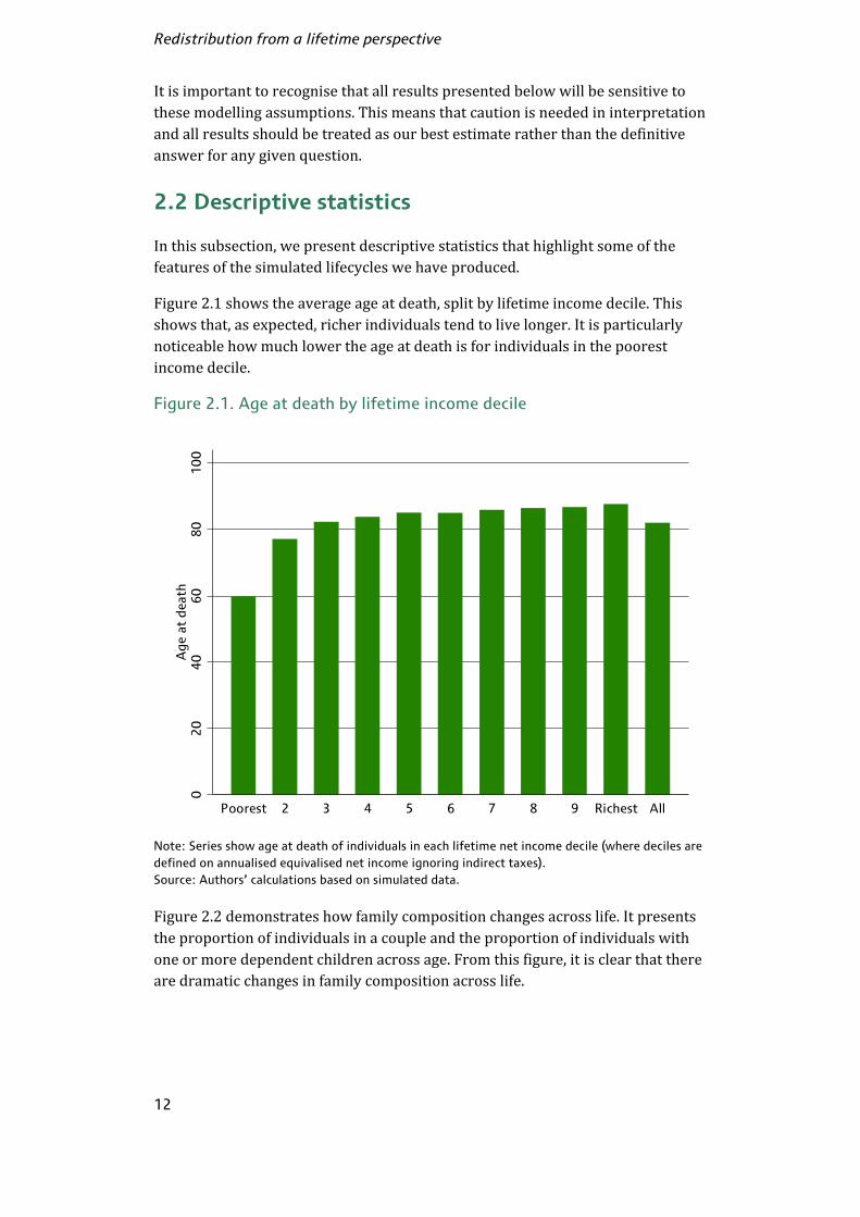
It is important to recognise that all results presented below will be sensitive to these modelling assumptions. This means that caution is needed in interpretation and all results should be treated as our best estimate rather than the definitive answer for any given question. 2.2 Descriptive statistics In this subsection, we present descriptive statistics that highlight some of the features of the simulated lifecycles we have produced. Figure 2.1 shows the average age at death, split by lifetime income decile. This shows that, as expected, richer individuals tend to live longer. It is particularly noticeable how much lower the age at death is for individuals in the poorest income decile. Figure 2.1. Age at death by lifetime income decile
Note: Series show age at death of individuals in each lifetime net income decile (where deciles are
defined on annualised equivalised net income ignoring indirect taxes).
Source: Authors’ calculations based on simulated data. Figure 2.2 demonstrates how family composition changes across life. It presents the proportion of individuals in a couple and the proportion of individuals with one or more dependent children across age. From this figure, it is clear that there are dramatic changes in family composition across life.
02
04
06
08
01
00
Ag
e a
t d
ea
th
Poorest 2 3 4 5 6 7 8 9 Richest All

Background and methodology
13
Figure 2.2. Family composition by age
Note: Series show the proportion of individuals in a couple and the proportion with at least one
dependent child by age.
Source: Authors’ calculations based on simulated data.
Figure 2.3. Employment rate by age and sex
Note: Series show proportions of individuals employed by age.
Source: Authors’ calculations based on simulated data.
0.2
.4.6
.8P
rop
ort
ion
20 40 60 80 100Age
Proportion couple Proportion with child
0.2
.4.6
.81
Pro
po
rtio
n e
mp
loy
ed
20 40 60 80Age
Males Females

Redistribution from a lifetime perspective
14
Figure 2.3 plots employment rates for men and women over life. Male employment rates are higher than female employment rates throughout life, but especially during the main child-rearing ages between 20 and 40. Both males and females withdraw gradually from the labour market between ages 50 and 75. Figure 2.4 shows how employment varies across the net income distribution. The cross-section series shows the proportion of working-age individuals who are employed, split by cross-sectional net income decile. The lifetime series shows the average fraction of working life that individuals are employed for, split by annualised lifetime net income decile. From this graph, it is clear that relatively few individuals in the bottom cross-sectional decile are employed (22%), but from a lifetime perspective, individuals in the bottom lifetime decile are employed for the majority of working life (an average of 66%).3 Figure 2.5 plots mean annual earnings (not conditional on working) and mean private pensions (not conditional on receiving a pension) across life for men and Figure 2.4. Employment among working age individuals by net income
decile
Note: The cross-section series shows the fraction of working-age individuals in each net income
decile who are employed (deciles are defined using the whole population, not just working-age
individuals). The lifetime series shows the average fraction of working life that individuals are
employed for. Working age is defined as under 63 for women and under 65 for men. Deciles are
defined on equivalised net income ignoring indirect taxes (annualised net income for lifetime
deciles).
Source: Authors’ calculations based on simulated data. 3 We may slightly overstate mobility in employment – see Section 2.1. If so, this latter figure is likely to be a
slight overstatement.
0.2
.4.6
.81
Pro
po
rtio
n e
mp
loy
ed
Poorest 2 3 4 5 6 7 8 9 Richest All
Cross-section Lifetime

Background and methodology
15
women. This shows that, on average, earnings rise for men until the late 40s and then decline steadily thereafter. For women, earnings flatten off during the late 20s, associated with taking time out of the labour market for child-rearing. They then rise again, reaching a peak at around age 50 before falling again towards retirement. As earnings decline around retirement, individuals start receiving private pensions, though at a much lower level, on average, than earnings during working life. Figure 2.5. Mean earnings and pensions by age and sex
Note: Series show mean earnings and private pensions across life. Values are expressed in real
2015 terms (deflated by the Retail Prices Index, or RPI). Earnings are zero for the unemployed and
for those not in receipt of a private pension.
Source: Authors’ calculations based on simulated data. Figure 2.6 plots the distributions for gross lifetime and cross-sectional incomes. The average gross income in the cross-section is £19,000 (recall that the only incomes considered here are earnings and private pensions). The average present value of lifetime incomes is £1.9 million.4 Both distributions exhibit positive skew, with long tails of individuals with high incomes. However, the skew is much more evident in the cross-section. This reflects the impact of income mobility on the lifetime distribution – a point to which we return below. 4 The figure for the average lifetime is coincidentally around 100 times that of the average cross-sectional
income. This is the case even though most of our simulated individuals live less than 100 years because the lifetime figure is present discounted value (weighting incomes received earlier in time more than those received later).
01
00
00
20
00
03
00
00
Inco
me
(£
20
15
)
20 40 60 80 100Age
Earnings (males) Earnings (females)
Private pensions (males) Private pensions (females)

Redistribution from a lifetime perspective
16
Figure 2.6. Gross income distributions
Note: The series show the densities of gross equivalised household incomes over the lifetime and
in a cross-section. Lifetime incomes are expressed in 2015 present value terms. We exclude the
top 1% of incomes and those with zero incomes.
Source: Authors’ calculations based on simulated data. Figure 2.7 shows how means-tested benefit entitlement varies by net income decile. The cross-section series shows the fraction of individuals in each net income decile who belong to a family entitled to means-tested benefits. The lifetime series shows the average fraction of life that individuals belong to a family entitled to means-tested benefits. This graph shows that more than 80% of the bottom three deciles are entitled to means-tested benefits in the cross-section, with entitlement much lower among deciles further up the distribution. Over the lifetime, the proportion of life for which individuals are entitled to means-tested benefits is more evenly spread across the deciles. Indeed, those in the richest decile of the lifetime income distribution spend almost one-fifth of their lifetime entitled to one of the main means-tested benefits.5
5 Note this may be an overestimate because we may slightly overstate the degree of mobility in employment
and earnings (see Section 2.1) and because we do not model assets rules in benefits (see Appendix A).
0.0
00
2.0
00
4.0
00
6D
en
sity
(li
feti
me)
0.0
00
01
.00
00
2.0
00
03
De
nsi
ty (
cro
ss-s
ect
ion
)
0 1000 2000 3000 4000 5000Gross income (lifetime) (£k PV 2015)
0 20000 40000 60000 80000Gross income (cross-section) (£ 2015)
Cross-section Lifetime

Background and methodology
17
Figure 2.7. Means-tested benefit entitlement by net income decile
Note: The cross-section series shows the fraction of individuals in each net income decile who
belong to a family entitled to means-tested benefits. The lifetime series shows the average
fraction of life that individuals belong to a family entitled to means-tested benefits. Deciles are
defined on equivalised net income ignoring indirect taxes (annualised net income for lifetime
deciles).
Source: Authors’ calculations based on simulated data. Figure 2.8 gives an indication of how persistent net income is over time. It plots the proportion of life spent in each cross-section net income decile by individuals in the poorest/richest lifetime net income decile. This shows that those lifetime poor/rich spend quite a substantial fraction of life outside the poorest/richest cross-sectional decile; in other words, there is a substantial degree of mobility around the distribution across life. It also shows that persistence is greater at the top of the distribution than at the bottom: individuals in the richest lifetime decile spend more of their time in the richest cross-sectional decile than individuals in the poorest lifetime decile spend in the poorest cross-sectional decile (35% compared to 22%).6
6 We may slightly overstate mobility in employment and earnings – see Section 2.1. If so, these figures are
likely to be slight understatements.
0.2
.4.6
.81
Pro
po
rtio
n e
nti
tle
d t
o m
ea
ns-
test
ed
ben
efi
ts
Poorest 2 3 4 5 6 7 8 9 Richest All
Cross-section Lifetime

Redistribution from a lifetime perspective
18
Figure 2.8. Proportion ever observed in poorest/richest snapshot decile,
by lifetime net income decile
Note: The series show the proportion of life spent in each cross-section net income decile by
individuals in the poorest/richest lifetime net income decile. Deciles are defined on equivalised net
income ignoring indirect taxes (annualised net income for lifetime deciles).
Source: Authors’ calculations based on simulated data.
0.1
.2.3
.4P
rop
ort
ion
of
life
in
each
cro
ss-s
ecti
on
al
de
cile
Poorest 2 3 4 5 6 7 8 9 Richest
Poorest lifetime decile Richest lifetime decile

19
© Institute for Fiscal Studies
3. Redistribution achieved by the current
tax and benefit system
In this section, we present our results on redistribution achieved by the current (2015/16) tax and benefit system for the baby-boom cohort. 3.1 How do taxes and benefits evolve across life? Figures 3.1 and 3.2 show how taxes and benefits evolve across life, on average, for the baby-boom cohort. Series are on an annual per-individual basis, assuming equal sharing in couples (i.e. family amounts divided by two), and are expressed in real 2015 terms (deflated by the RPI). Figure 3.1. Mean taxes by age, split by taxes
Note: Series are calculated on an annual per-individual basis, assuming equal sharing in couples
(i.e. family amounts divided by two), and are expressed in real 2015 terms (deflated by the RPI).
Series assume that individuals face the 2015/16 tax and benefit system throughout life uprated in
line with average earnings (the Average Earnings Index, or AEI). Means are calculated across all
individuals alive at each age, trimming the top and bottom 1% of the distribution to avoid outliers
affecting the series unduly.
Source: Authors’ calculations based on simulated data. In Figure 3.1, mean taxes peak at £10,800 per year for individuals in their early 50s and then fall back to below £4,700 per year by age 75. The peak is due to a combination of income tax, National Insurance and indirect tax. There is no discrete fall in taxes at the state pension age (63 for women and 65 for men in the 2015/16 system) for two main reasons. First, individuals in our simulations
02
46
81
0M
ea
n a
nn
ua
l ta
xe
s £
k (
20
15
)
20 40 60 80 100Age
Income tax National Insurance
Council tax VAT
Other indirect tax

Redistribution from a lifetime perspective
20
withdraw from the labour force fairly gradually after age 50 (see Figure 2.3). Second, as individuals leave work, they start receiving pensions (see Figure 2.5), which are subject to income tax. National Insurance plays a limited role after state pension age because it is not levied on unearned income. Note, however, that our simulations do not capture the top of the income distribution very well and this is likely to affect these mean tax figures because rich individuals tend to pay a lot of tax. Figure 3.2 shows how the main welfare benefits evolve across life on average. Individuals also benefit from public service spending, but this is excluded from this analysis (but see Appendix E, which includes health and education spending). Mean benefits are low throughout working life (below £2,500 per year). There is a slight hump during the main child-rearing years that is due to support targeted towards families with children (in the form of child benefit and child tax credit). After state pension age, there is a substantial rise in mean benefits to a little over £7,500 per year. This is almost exclusively due to state pensions. Mean benefits then continue to rise steadily during retirement, primarily because uprating the Figure 3.2. Mean benefits by age, split by benefits
Note: ‘Income support’ includes jobseeker’s allowance, employment support allowance and
pension credit. Series are calculated on an annual per-individual basis, assuming equal sharing in
couples (i.e. family amounts divided by two), and are expressed in real 2015 terms (deflated by the
RPI). Series assume that individuals face the 2015/16 tax and benefit system throughout life
uprated in line with average earnings (AEI). Means are calculated across all individuals alive at
each age, trimming the top and bottom 1% of the distribution to avoid outliers affecting the
series unduly.
Source: Authors’ calculations based on simulated data.
05
10
15
20
Me
an
an
nu
al b
en
efi
ts £
k (
20
15
)
20 40 60 80 100Age
Income support Housing benefit
Council tax benefit Working tax credit
Child tax credit Child benefit
Disability living allowance State pensions
Winter fuel payment

Redistribution achieved by the current tax and benefit system
21
tax and benefit system in line with earnings increases the real value of state pensions each year.7 Figure 3.3 plots overall mean taxes and mean benefits, as well as the difference between the two, mean net benefits (benefits less taxes). Mean net benefits are negative (meaning individuals are net contributors on average) during working life and positive (meaning individuals are net recipients on average) during retirement. They reach their lowest value (greatest average net contribution) of around –£9,700 for individuals in their early 50s and achieve their highest value (greatest average net receipt) among the oldest individuals. This shows that there are pronounced lifecycle patterns for the times when individuals are net contributors and when they are net recipients: lifecycle variation is an important reason why some individuals are net recipients at a point in time. Net benefits are, on average, negative over the whole of life as the state collects more in the taxes we include than it spends on benefits (taxes account for the vast majority of government receipts but benefits are only around 30% of government spending). Figure 3.3. Mean taxes, benefits and net benefits by age
Note: Series are calculated on an annual per-individual basis, assuming equal sharing in couples
(i.e. family amounts divided by two), and are expressed in real 2015 terms (deflated by the RPI).
Series assume that individuals face the 2015/16 tax and benefit system throughout life uprated in
line with average earnings (AEI). Means are calculated across all individuals alive at each age,
trimming the top and bottom 1% of the distribution to avoid outliers affecting the series unduly.
Source: Authors’ calculations based on simulated data. 7 There are also a number of less important reasons why mean benefits rise during retirement. These include:
(i) individuals with higher state pension entitlement tend to live longer; (ii) some individuals inherit state pension entitlement when their partner dies; (iii) older individuals are more likely to be receiving disability benefits; (iv) the winter fuel payment rises with age.
-20
-15
-10
-50
51
01
52
0M
ea
n a
nn
ua
l ta
xe
s a
nd
be
ne
fits
(£
k 2
01
5)
20 40 60 80 100Age
Taxes Benefits Net benefits

Redistribution from a lifetime perspective
22
3.2 How do net contributions vary across
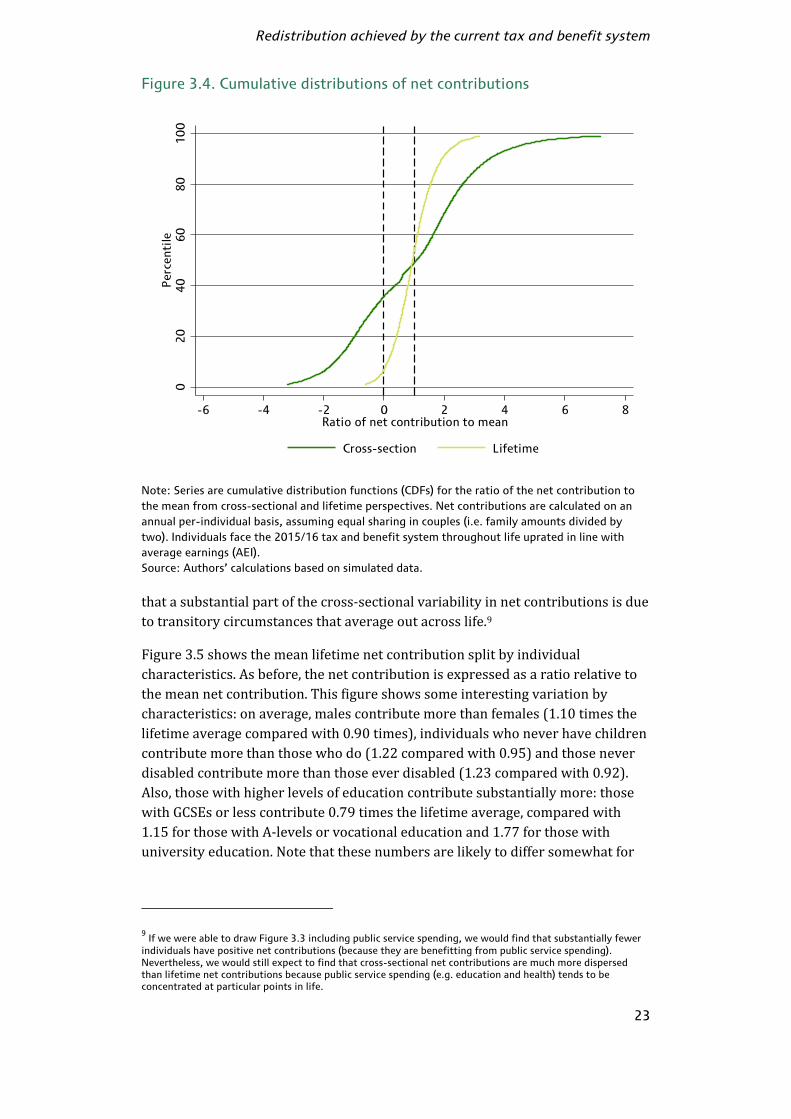
individuals? In Section 3.1, we considered averages across all individuals. In this subsection, we compare how net contributions (taxes less benefits, i.e. the negative of net benefits) vary across individuals from a cross-sectional and lifetime perspective. Statistics relating to the cross-section are calculated using a synthetic 2015/16 cross-section that describes what the population would look like if all cohorts were the same as the baby-boom cohort (see Section 2.1 for more details). From a cross-sectional perspective, the overall mean net contribution for the baby-boom cohort is £4,160 per year in 2015 prices; from a lifetime perspective, it is £494,000 in PV 2015 terms.8 Again, the mean net contribution is positive from both a cross-sectional and lifetime perspective because the tax and benefit system raises net revenue. These average values mask wide variation across individuals. Figure 3.4 plots cumulative distributions for the ratio of the net contribution relative to the mean from cross-sectional and lifetime perspectives. The x-axis is the net contribution expressed as a proportion of the mean net contribution (so 0 means no net contribution, 1 means a net contribution equal to the mean, 2 means a net contribution of double the mean, and so on). The y-axis shows the proportion of individuals with net contributions at or below the corresponding x-axis value. So, for example, almost half of individuals have a cross-sectional net contribution ratio of no more than 1 (i.e. a net contribution at or below the mean net contribution), and therefore slightly more than half have a contribution of greater than 1. This cross-section line is much flatter than the lifetime line, indicating that cross-sectional net contributions are much more dispersed than lifetime net contributions. For example, from a cross-sectional perspective, 36% of individuals are net recipients (i.e. have a negative net contribution ratio) but, from a lifetime perspective, only 7% are. This means that many individuals who are net recipients at a point in time will nevertheless end up being net contributors over the lifetime. Likewise, from a cross-sectional perspective, 33% have a net contribution relative to the mean of between 0 and 2 (i.e. positive but no more than twice the mean net contribution), while for the lifetime the figure is 85%. Around 50% of individuals have net contributions that exceed the mean regardless of which perspective is taken. The fact that cross-sectional net contributions are much more dispersed than lifetime net contributions means 8 The cross-sectional mean net contribution (£4,160) is not equal to the lifetime figure (£494,000) divided by
the average length of adult life. This is for two reasons. First, the lifetime figure is the present value of annual contributions, and this assigns greater weight to contributions that are made earlier in time (payments for individuals at different ages in the cross-section are made at the same point in time so are weighted equally). Second, individuals face different parameters of the tax and benefit system at different ages under the lifetime calculation.
Redistribution achieved by the current tax and benefit system
23
Figure 3.4. Cumulative distributions of net contributions
Note: Series are cumulative distribution functions (CDFs) for the ratio of the net contribution to
the mean from cross-sectional and lifetime perspectives. Net contributions are calculated on an
annual per-individual basis, assuming equal sharing in couples (i.e. family amounts divided by
two). Individuals face the 2015/16 tax and benefit system throughout life uprated in line with
average earnings (AEI).
Source: Authors’ calculations based on simulated data. that a substantial part of the cross-sectional variability in net contributions is due to transitory circumstances that average out across life.9 Figure 3.5 shows the mean lifetime net contribution split by individual characteristics. As before, the net contribution is expressed as a ratio relative to the mean net contribution. This figure shows some interesting variation by characteristics: on average, males contribute more than females (1.10 times the lifetime average compared with 0.90 times), individuals who never have children contribute more than those who do (1.22 compared with 0.95) and those never disabled contribute more than those ever disabled (1.23 compared with 0.92). Also, those with higher levels of education contribute substantially more: those with GCSEs or less contribute 0.79 times the lifetime average, compared with 1.15 for those with A-levels or vocational education and 1.77 for those with university education. Note that these numbers are likely to differ somewhat for 9 If we were able to draw Figure 3.3 including public service spending, we would find that substantially fewer
individuals have positive net contributions (because they are benefitting from public service spending). Nevertheless, we would still expect to find that cross-sectional net contributions are much more dispersed than lifetime net contributions because public service spending (e.g. education and health) tends to be concentrated at particular points in life.
02
04
06
08
01
00
Pe
rce
nti
le
-6 -4 -2 0 2 4 6 8Ratio of net contribution to mean
Cross-section Lifetime
Redistribution from a lifetime perspective
24
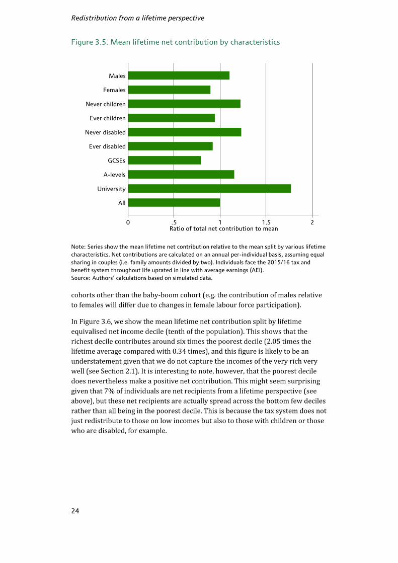
Figure 3.5. Mean lifetime net contribution by characteristics
Note: Series show the mean lifetime net contribution relative to the mean split by various lifetime
characteristics. Net contributions are calculated on an annual per-individual basis, assuming equal
sharing in couples (i.e. family amounts divided by two). Individuals face the 2015/16 tax and
benefit system throughout life uprated in line with average earnings (AEI).
Source: Authors’ calculations based on simulated data. cohorts other than the baby-boom cohort (e.g. the contribution of males relative to females will differ due to changes in female labour force participation). In Figure 3.6, we show the mean lifetime net contribution split by lifetime equivalised net income decile (tenth of the population). This shows that the richest decile contributes around six times the poorest decile (2.05 times the lifetime average compared with 0.34 times), and this figure is likely to be an understatement given that we do not capture the incomes of the very rich very well (see Section 2.1). It is interesting to note, however, that the poorest decile does nevertheless make a positive net contribution. This might seem surprising given that 7% of individuals are net recipients from a lifetime perspective (see above), but these net recipients are actually spread across the bottom few deciles rather than all being in the poorest decile. This is because the tax system does not just redistribute to those on low incomes but also to those with children or those who are disabled, for example.
0 .5 1 1.5 2Ratio of total net contribution to mean
All
University
A-levels
GCSEs
Ever disabled
Never disabled
Ever children
Never children
Females
Males

Redistribution achieved by the current tax and benefit system
25
Figure 3.6. Mean lifetime net contribution by lifetime income decile
Note: Series show the mean lifetime net contribution relative to the mean, split by lifetime net
income decile (and where deciles are defined on equivalised net income ignoring indirect taxes).
Net contributions are calculated on an annual per-individual basis, assuming equal sharing in
couples (i.e. family amounts divided by two). Individuals face the 2015/16 tax and benefit system
throughout life uprated in line with average earnings (AEI).
Source: Authors’ calculations based on simulated data.
3.3 How much redistribution is effectively across
periods of life rather than across individuals? In Section 3.2, we noted that net contributions (taxes less benefits) are much more dispersed from a cross-sectional perspective than a lifetime perspective. This suggests that part of what the tax and benefit system does cancels out across life (i.e. redistribution is towards individuals in some periods and away from them in other periods). In this subsection, we consider the extent to which this is the case for the baby-boom cohort. We present the formal decomposition in Appendix A but here we develop it in steps. We estimate that, on average across individuals, total lifetime (direct and indirect) taxes amount to £776,000 in 2015 PV terms or 45.4% of gross lifetime income. The corresponding figure for benefits is £281,000 or 16.5% of gross lifetime income. Taking the difference between taxes and benefits gives an average net contribution of £494,000 (this number was cited in the previous subsection). This is the average revenue raised per individual across life in PV 2015 terms.
0 .5 1 1.5 2Ratio of total net contribution to mean
All
Richest
9
8
7
6
5
4
3
2
Poorest
Lif
eti
me
eq
uiv
ali
sed
ne
t in
co
me
de
cil
e

Redistribution from a lifetime perspective
26
This revenue can be raised in a way that is redistributive or not. We consider two alternative definitions of what counts as being not redistributive: where the net contribution is either a constant lump-sum amount for each individual in each period or a constant proportion of gross income for each individual in each period. We define redistribution in any given period as the individual’s net contribution less the no-redistribution baseline. (Note, therefore, that redistribution need not be inequality-reducing – we address the ability of the tax and benefit system to reduce inequality in Sections 3.4 and 3.5.) If we sum redistribution in PV 2015 terms across all individuals, the answer will be zero because the no-redistribution baseline is chosen to raise the same revenue as the actual tax and benefit system. However, if we ignore minus signs when doing the calculation (i.e. calculate the modulus) and divide by the number of individuals, we will find the average amount of redistribution (either towards or away from individuals) achieved per individual by the tax and benefit system. Doing this, we find that the 2015/16 system does an average of £688,000 of redistribution per individual in PV 2015 terms (40.3% as a proportion of gross lifetime income) if the lump-sum baseline is used. This is lower than total lifetime taxes (£776,000) because taxes and benefits often partially offset within a given year. Under the proportional baseline, the amount is much lower: £345,000 (20.2% of gross lifetime income). The reason this amount is much lower is that the tax and benefit system is much closer to being a proportional system than a lump-sum system, so less redistribution happens relative to a proportional baseline. Some redistribution nets off across life (i.e. redistribution is positive in some periods and negative in others) leaving lifetime income unchanged. This can be thought of as redistributing across periods of life so we label it ‘intrapersonal’ redistribution. Under a lump-sum baseline, we estimate that average intrapersonal redistribution per individual is £390,000 in PV 2015 terms (22.9% of gross lifetime income) or 56.6% as a proportion of total redistribution. That is to say that 56.6% of redistribution nets off across life. Under a proportional baseline, average intrapersonal redistribution per individual is £205,000 in PV 2015 terms (12.0% of gross lifetime income) or 59.4% as a proportion of total redistribution. Redistribution that does not net off across life but alters the level of lifetime net income can be thought of as redistribution across individuals, or ‘interpersonal’ redistribution. Under a lump-sum baseline, we estimate that average interpersonal redistribution per individual is £299,000 in PV 2015 terms (17.5% of gross lifetime income) or 43.4% as a proportion of total redistribution. Under a proportional baseline, average interpersonal redistribution per individual is £140,000 in PV 2015 terms (8.2% of gross lifetime income) or 40.6% as a proportion of total redistribution.

Redistribution achieved by the current tax and benefit system
27
Therefore, we can conclude that, under either baseline, more than half of the redistribution achieved by the tax and benefit system is intrapersonal. This means that overall, for every £1 of redistribution received or withdrawn, more than half of it is offset in other periods of life. There is one important caveat to bear in mind: the calculations will be sensitive to the period of measurement (i.e. what counts as the ‘current age’). The longer this period is, the more taxes and benefits will offset at the current age and therefore will be disregarded. This will tend to reduce the share of intrapersonal redistribution. We work on an annual basis because income tax is assessed on an annual basis. In previous work (Roantree and Shaw, 2014), we calculated the intrapersonal share over periods shorter than a full lifetime. We found that it reached 10% after 15 years under both baselines.10 The fact that the share we calculate here is so much higher suggests that much of the redistribution across periods of life happens at a lower frequency than a 15-year horizon can easily capture (e.g. redistribution between periods with and without children and between working life and retirement). It is possible to calculate the share of redistribution that is intrapersonal separately for each individual. In Figure 3.7, we show how the mean intrapersonal share varies by lifetime characteristics. Both baselines show similar patterns across groups, so we focus here on the lump-sum baseline. There is little difference between males and females or between those never with children and those ever with children. Those never in a couple have a lower intrapersonal share that those ever in a couple (47.8% compared with 57.0%), probably because they tend to spend more periods in work and so are more consistently net contributors. Those never disabled have a lower share than those ever disabled (49.6% compared with 58.5%) because disability is associated with benefit receipt and time out of the labour market, and therefore more intrapersonal redistribution. And those with higher (university) education have a lower intrapersonal share than those with basic (GCSEs or less) or intermediate (A-levels or vocational) education (43.5% compared with 58.2 and 59.0%). This is because those with higher education tend to earn more across life (see Figure 3.5) so are more consistently net contributors.
10
Note that this figure is across the population as a whole and not just for the baby-boom cohort.

Redistribution from a lifetime perspective
28
Figure 3.7. Mean intrapersonal share by characteristics
Note: Series show the mean share of redistribution that is intrapersonal under a lump-sum and a
proportional baseline, split by various lifetime characteristics. Taxes and benefits are calculated on
an annual per-individual basis, assuming equal sharing in couples (i.e. family amounts divided by
two). Individuals face the 2015/16 tax and benefit system throughout life uprated in line with
average earnings (AEI).
Source: Authors’ calculations based on simulated data. In Figure 3.8, we plot the mean intrapersonal share by lifetime net income decile. This shows that the shares are highest among deciles 5–9, and considerably lower at the bottom and right at the top of the distribution. A hump-shape of this sort is what you would expect from a tax and benefit system that redistributes from rich to poor. Individuals in the richest decile have a low intrapersonal share (and therefore a high interpersonal share) because they contribute in excess of the no-redistribution baseline in more periods of life than other deciles. For individuals in the poorest deciles, the logic is similar: these individuals have a low intrapersonal share (and therefore a high interpersonal share) because they contribute less than the no-redistribution baseline in more periods of life than other deciles. In between (deciles 5–9), the contributions of individuals are sometimes above and sometimes below the no-redistribution baseline.
0 .2 .4 .6 .8 1Share of intrapersonal redistribution
All
University
A-levels
GCSEs
Ever disabled
Never disabled
Ever children
Never children
Ever couple
Never couple
Females
Males
Lump-sum Proportional

Redistribution achieved by the current tax and benefit system
29
Figure 3.8. Mean intrapersonal share by lifetime income decile
Note: Series show the mean share of redistribution that is intrapersonal under a lump sum and a
proportional baseline, split by lifetime net income decile (and where deciles are defined on
equivalised net income ignoring indirect taxes). Taxes and benefits are calculated on an annual
per-individual basis, assuming equal sharing in couples (i.e. family amounts divided by two).
Individuals face the 2015/16 tax and benefit system throughout life uprated in line with average
earnings (AEI).
Source: Authors’ calculations based on simulated data.
3.4 How effective is the tax and benefit system at
reducing inequality? Our analysis so far has not tackled inequality directly. In this subsection, we turn our attention to income inequality, assessing how unequally distributed incomes are, from cross-sectional and lifetime perspectives, and how effective the tax and benefit system is at mitigating both. We measure income inequality using the Gini coefficient, one of the most widely used measures of inequality. It takes on values between zero and one, with higher values corresponding to a greater degree of inequality. A value of zero means that everyone has the same income, while a value of one means that all income is concentrated in the hands of a single individual. The Gini coefficient can be interpreted as half the average income gap between all pairs of individuals, expressed as a proportion of average income.11 11
See Barr (2004) for an introduction and Sen (1973, 1992) for a fuller discussion.
0 .2 .4 .6 .8 1Share of intrapersonal redistribution
All
Richest
9
8
7
6
5
4
3
2
Poorest
Lif
eti
me
eq
uiv
ali
sed
ne
t in
co
me
de
cile
Lump-sum Proportional

Redistribution from a lifetime perspective
30
Table 3.1 gives gross and net income Gini coefficients calculated for the synthetic cross-section and on a lifetime basis for the baby-boom cohort. First note how much lower inequality is over the lifetime: the cross-section Gini coefficient for gross income is 0.493 compared with 0.281 across the whole of adult life. This indicates that a lot of the income inequality before taxes and benefits between individuals is temporary, either reflecting the stage of life they are at (such as differences in work experience and family structure – see Figure 2.2) or reflecting transitory shocks individuals have experienced (such as unemployment). Table 3.1. Gross and net income Gini coefficients
Horizon Gross income Net income Net income less indirect taxes
Cross-section 0.493 0.298 0.337
Lifetime 0.281 0.224 0.239
Note: Taxes and benefits are calculated on an annual basis and are equivalised using the Modified
OECD equivalence scale. The ‘Net income’ column excludes the effect of indirect taxes, while the
‘Net income less indirect taxes’ column subtracts them. Individuals face the 2015/16 tax and
benefit system throughout life uprated in line with average earnings (AEI).
Source: Authors’ calculations based on simulated data. The second thing to notice is that the tax and benefit system is effective at reducing inequality, but more so in the cross-section: when including the effect of indirect taxes, the cross-section Gini falls from 0.493 to 0.337, a reduction of 0.155 (or 31.4%) while the lifetime Gini falls from 0.281 to 0.239, a reduction of 0.042 (or 14.9%, which is less than half the corresponding cross-sectional fall). This reflects the fact that much of what the tax and benefit system does is intrapersonal redistribution (see Section 3.3). The reason for this is that most taxes and benefits are assessed over periods of a year or less, making it much easier to target outcomes over short horizons. It is interesting to compare Gini coefficients for our synthetic cross-section with those calculated on an actual cross-section. The gross income Gini reported here of 0.493 compares with 0.565 based on the 2012 LCFS (see Appendix F) and 0.528 based on the Family Resources Survey (FRS). The net income Gini here of 0.298 compares with 0.301 for the 2012 LCFS (see Appendix F) and 0.343 for the FRS (see Belfield et al., 2015). It is hard to tell a consistent story to explain these differences (and, indeed, they might partly reflect modelling assumptions and sampling variation). However, the FRS numbers may be higher than the synthetic cross-section because the FRS has better coverage of the very well off, thanks to a larger sample, uncensored earnings and further adjustments to account for known under-sampling of the very rich. Another potential explanation for differences between actual and synthetic data is the fact that actual cross-sections include many generations (not just the baby-boom cohort), so will incorporate generational differences. This could include differences in within-cohort inequality across generations, or intergenerational inequality. Figure 3.9 plots concentration curves for net revenue from both cross-sectional and lifetime perspectives. These concentration curves show the cumulative

Redistribution achieved by the current tax and benefit system
31
Figure 3.9. Concentration curve for net revenue
Note: Series are concentration curves for net revenue from cross-sectional and lifetime
perspectives. These curves show the cumulative proportion of net revenue accounted for by
individuals ranked from poorest to richest on the basis of equivalised net cross-section or lifetime
income (ignoring indirect taxes). Taxes and benefits are calculated on an annual basis and are
equivalised using the modified OECD equivalence scale. Individuals face the 2015/16 tax and
benefit system throughout life uprated in line with average earnings (AEI).
Source: Authors’ calculations based on simulated data. proportion of net revenue accounted for by individuals ranked from poorest to richest on the basis of net cross-section or lifetime income. If the concentration curve falls on the 45 degree line, then each individual contributes an equal amount to net revenue. As it is, both curves fall below the 45 degree line, and the cross-section curve substantially more so than the lifetime curve. The regions where the curves go negative indicate that individuals are net recipients rather than net contributors to government revenue. From this figure, we can say that contributions to net revenue are significantly more concentrated in the cross-section than over the lifetime. For example, in the cross-section, the top 20% of individuals contribute 79% of total net revenue, while across the lifetime, the top 20% of individuals contribute 39% of total net revenue. It is important to recognise, however, that both these values are likely to understate concentration at the top because a lot of tax revenue comes from the very rich who we do not capture very well (see Section 2). The fact that the tax and benefit system achieves a smaller reduction in inequality from a lifetime perspective is partly because there is less inequality to reduce from a lifetime perspective, but it is also a consequence of the fact that taxes and benefits are assessed on periods of a year or less, meaning they are (inevitably) less well targeted at reducing lifetime inequality than snapshot inequality.
-.5
0.5
1C
um
ula
tive %
to
tal re
ven
ue
0 .2 .4 .6 .8 1Proportion of individuals
Cross-section Lifetime

Redistribution from a lifetime perspective
32
3.5 Which taxes and benefits are most effective at
reducing inequality? In Section 3.4, we have shown that the tax and benefit system reduces inequality both from a cross-sectional and a lifetime perspective. This raises the question that we address in this subsection: which taxes and benefits are most effective at reducing inequality? As a starting point, we consider what impact benefits, direct taxes and indirect taxes have on the Gini coefficient for the baby-boom cohort. This is set out in Table 3.2, which describes how the Gini coefficient changes as each income source is added in sequence from a cross-sectional perspective (i.e. based on our synthetic 2015/16 cross-section) and from a lifetime perspective.12 Table 3.2. Effect of each income source on the Gini coefficient
Cross-section Lifetime
Level Change Prop. change
Level Change Prop. change
Gross income 0.493 0.281
Total benefits 0.340 –0.153 –0.311 0.241 –0.040 –0.143
Income support 0.476 –0.017 –0.035 0.273 –0.008 –0.028
Housing benefit 0.461 –0.014 –0.030 0.268 –0.005 –0.020
Council tax benefit 0.451 –0.010 –0.023 0.264 –0.003 –0.012
Working tax credit 0.447 –0.004 –0.009 0.262 –0.002 –0.009
Child tax credit 0.438 –0.009 –0.020 0.255 –0.007 –0.025
Child benefit 0.435 –0.003 –0.008 0.252 –0.003 –0.013
Disability living allow. 0.424 –0.011 –0.025 0.250 –0.002 –0.010
State pensions 0.341 –0.083 –0.196 0.241 –0.009 –0.035
Winter fuel payment 0.340 –0.001 –0.004 0.241 0.000 0.000
Total direct taxes 0.298 –0.041 –0.122 0.224 –0.017 –0.070
Income tax 0.299 –0.041 –0.120 0.222 –0.019 –0.078
National insurance 0.286 –0.012 –0.042 0.220 –0.002 –0.010
Council tax 0.298 0.012 0.042 0.224 0.004 0.019
Total indirect taxes 0.338 0.039 0.132 0.239 0.015 0.069
VAT 0.322 0.024 0.081 0.232 0.008 0.037
Other indirect taxes 0.338 0.015 0.047 0.239 0.007 0.031
Note: ‘Income support’ includes jobseeker’s allowance, employment support allowance and
pension credit. Individuals face the 2015/16 tax and benefit system throughout life uprated in line
with average earnings (AEI).
Source: Authors’ calculations based on simulated data.
12
Adding income sources in sequence as we do here means that the results are dependent on the ordering we
have chosen. We have experimented with adding income sources in reverse. This makes some difference to the results, such as making income tax and National insurance closer to having no effect on inequality, but most patterns are preserved.

Redistribution achieved by the current tax and benefit system
33
From a cross-sectional perspective, the gross income Gini coefficient is 0.493. The addition of all benefits reduces it to 0.340 (a fall of 0.153 or 31.1%). Direct taxes take it down further to 0.298 (a fall of 0.041 or 12.2%), while indirect taxes increase it back up to 0.338 (a rise of 0.039 or 13.2%). These results are based on our synthetic 2015/16 cross-section, but they display a very similar pattern to those reported by ONS (2015) for 2013/14 (the most recent year available) that are based on actual cross-section data derived from the LCFS. Turning to individual income sources, state pensions account for more than half of the reduction in the Gini coefficient due to benefits (a fall of 0.083 out of a total of 0.153), in large part because they are the single biggest benefit. Income tax accounts for almost the total fall in the Gini due to direct taxes (the redistributive effects of National Insurance (progressive) and council tax (regressive) roughly cancel). VAT increases cross-sectional inequality more than other indirect taxes (increasing the Gini by 8.1% compared to 4.7%). Again, this is largely due to the fact that individuals pay substantially more VAT than they pay in other indirect taxes. From a lifetime perspective, the picture is somewhat different. The Gini coefficient for gross income is 0.281. The addition of benefits takes it down to 0.241 (a fall of 0.040 or 14.3%), the subtraction of direct taxes reduces it to 0.224 (a fall of 0.017 or 7.0%), while the subtraction of indirect taxes gives 0.239 (a rise of 0.015 or 6.9%). Thus, in proportional terms, benefits are less effective at reducing lifetime inequality than they are at reducing cross-sectional inequality (a 14.3% fall compared with 31.1%) and direct taxes somewhat less effective (a 7.0% fall compared with 12.2%). Indirect taxes increase lifetime inequality by somewhat less than they increase cross-sectional inequality (6.9% compared with 13.2%). Looking at how much individual benefits reduce lifetime inequality, state pensions reduce it the most (partly because they are the biggest benefit) – as with the cross-section – but now they account for only a quarter of the total fall due to benefits (compared with more than half in the cross-section). This reflects the fact that pensioners tend to have low gross private incomes in the cross-section (see Figure 2.5) but this will not be true over the lifetime because the majority of people are pensioners at some point in their lives. VAT increases lifetime inequality by less (in proportional terms) than cross-sectional inequality: 3.7% compared to 8.1%. This is a consequence of income and spending patterns across the distribution. Many of the individuals at the bottom of the cross-sectional income distribution have temporarily low incomes and so have high expenditure relative to their income. As a result, indirect taxes are large as a proportion of snapshot income, making them look quite regressive. By contrast, VAT is less regressive from a lifetime perspective because the differences between lifetime income and lifetime consumption do not vary so much between rich and poor. Indeed, if income and expenditure were equal over the lifetime, then we would expect VAT to have little effect on lifetime inequality. The main reason why VAT remains regressive from a lifetime perspective is that

Redistribution from a lifetime perspective
34
in our simulations the lifetime rich consume a smaller fraction of their lifetime income than the lifetime poor (which is possible if, for example, the lifetime rich leave more in the way of inheritances). As a result, VAT remains slightly larger as a proportion of income for the lifetime poor than the lifetime rich. We must be a little tentative over this conclusion, however, because our simulations are only based on cross-sectional consumption information, so it is hard to draw definitive conclusions about lifetime consumption patterns.13 The results so far have been based on a sequential approach where we start with gross income and then incorporate each tax and benefit one at a time. This is easy to understand but has the disadvantage that the order in which income sources are included potentially matters (as noted above). An alternative is to ask how the Gini coefficient would change in response to a 1% increase in each income source for each individual. This can be done using a method proposed in Lerman and Yitzhaki (1985). This is what we do in Table 3.3, from a cross-section and a lifetime perspective. Unlike the results presented in Table 3.2, the calculation does not depend on the order in which each income source is considered.14 These results are broadly consistent with those in Table 3.2. Again, we note several differences between the effects of taxes and benefits on cross-sectional inequality and lifetime inequality. Both direct taxes and benefits appear more inequality-reducing in the cross-section compared to the lifetime. A 1% increase in all direct taxes results in a 0.134% decrease in cross-sectional inequality but only a 0.085% reduction in lifetime inequality. Similarly, a 1% increase in all benefits results in a 0.417% reduction in cross-sectional inequality but only a 0.184% reduction in lifetime inequality. As we saw in Table 3.2, indirect taxes appear less regressive when their effects are viewed over the lifetime. A 1% increase in indirect taxes leads to a 0.158% increase in cross-sectional inequality as compared to a 0.087% increase in lifetime inequality. Increases in VAT in particular only increase inequality half as much (by 0.054% compared to 0.109%) when a lifetime perspective is taken. These figures for the effects of indirect taxes should be treated tentatively given the issues surrounding the consumption data we noted above.
13
There is an ongoing debate about whether those with higher lifetime incomes also have higher lifetime
savings (and hence spend a smaller proportion of their lifetime incomes). Using UK and US data, Bozio et al. (2013) find that the lifetime rich appear to save more.
14 Note that this does not account for any interactions between taxes and benefits (e.g. an increase in child tax
credit decreases housing benefit entitlement for some people).

Redistribution achieved by the current tax and benefit system
35
Table 3.3. Effect on Gini coefficient (× 100) of a 1% increase in each
income source
Tax/benefit Cross-section
Lifetime
Change Prop. change
Change Prop. change
Gross income 0.133 0.393 0.044 0.183
Total benefits –0.141 –0.417 –0.044 –0.184
Income support –0.021 –0.062 –0.009 –0.036
Housing benefit –0.010 –0.029 –0.005 –0.021
Council tax benefit –0.012 –0.036 –0.004 –0.016
Working tax credit –0.006 –0.018 –0.003 –0.012
Child tax credit –0.013 –0.038 –0.008 –0.033
Child benefit –0.006 –0.017 –0.004 –0.018
Disability Living Allowance –0.006 –0.017 –0.003 –0.011
State pensions –0.066 –0.195 –0.009 –0.037
Winter fuel payment –0.002 –0.005 0.000 –0.001
Total direct taxes –0.045 –0.134 –0.020 –0.085
Income tax –0.053 –0.158 –0.026 –0.109
National insurance –0.011 –0.032 –0.001 –0.005
Council tax 0.019 0.055 0.007 0.029
Total indirect taxes 0.053 0.158 0.021 0.087
VAT 0.037 0.109 0.013 0.054
Other indirect taxes 0.016 0.049 0.008 0.032
Note: All values have been multiplied by 100. ‘Income support’ includes jobseeker’s allowance,
employment support allowance and pension credit. Individuals face the 2015/16 tax and benefit
system throughout life uprated in line with average earnings (AEI).
Source: Authors’ calculations based on simulated data. The results in Table 3.3 show how big a change in inequality a 1% change in each tax and benefit produces. A 1% change in large taxes or benefits (such as state pensions) will tend to have a bigger impact than a 1% change in smaller taxes or benefits (such as the winter fuel payment) because it implies a bigger change in spending. A different – and important – question is: if it wanted to, where should the government spend a fixed sum of money to reduce inequality by the most? This is the question we tackle in Section 5.1.

Redistribution from a lifetime perspective
36
3.6 Summary In this section, we have shown how our impression of the current tax and benefit system changes once we take a lifetime perspective rather than the standard cross-sectional point of view. Our main findings are as follows. Mean net benefits (benefits less taxes) have a pronounced pattern of across the lifecycle, being on average negative (i.e. taxes exceed benefits) during working life and positive during retirement (i.e. benefits exceed taxes). There is wide variation in net contributions (taxes less benefits) across individuals but cross-sectional net contributions are much more dispersed than lifetime net contributions. 36% of individuals have negative net contributions in the cross-section but only 7% do over the lifetime. More than half – 56.6% using a lump-sum baseline – of the redistribution that the tax and benefit system achieves is ‘intrapersonal’ (i.e. effectively across periods of life). In other words, overall, for every £1 of redistribution received or withdrawn, more than half of it is offset in other periods of life. Inequality is much lower from a lifetime than a cross-sectional perspective: the cross-section gross income Gini coefficient is 0.493 compared with 0.281 across the whole of adult life. This indicates that a lot of the inequality between individuals is temporary in nature, either reflecting the stage of life they are at or the transitory shocks they have experienced. The tax and benefit system is less effective at reducing inequality over the lifetime than in the cross-section. In the cross-section, it reduces the Gini coefficient by 31.4% but over the lifetime only by 14.9%. This reflects the fact that much of what the tax and benefit does is intrapersonal redistribution. The reason for this is that most taxes and benefits are assessed over periods of a year or less, making it much easier to target outcomes over short horizons. Benefits are less effective at reducing lifetime inequality than cross-sectional inequality (leading to a 14.3% fall compared with 31.1%) and direct taxes somewhat less effective (a 7.0% fall compared with 12.2%). Indirect taxes increase lifetime inequality by somewhat less than they increase cross-sectional inequality (6.9% compared with 13.2%). Among all the taxes and benefits we consider, state pensions are most effective at reducing inequality, but they are much more effective at reducing cross-sectional inequality (a 19.6% fall) than lifetime inequality (a 3.5% fall). This reflects the fact that pensioners tend to have low gross private incomes in the cross-section but not over the lifetime because the majority of people are pensioners at some point in their lives.
37
© Institute for Fiscal Studies
4. Distributional effects of historical tax
and benefit reforms
In this section, we present our results on redistribution achieved by historical tax and benefit systems, and reforms made to these systems. In these results, we describe reforms as being progressive or regressive. We say that a reform is progressive if the average gain is smaller (or the loss larger) as a proportion of income for individuals higher up the income distribution. Conversely, a reform is regressive if the gain is larger (or the loss smaller) as a proportion of income for individuals higher up the income distribution. 4.1 How have reforms to the tax and benefit system
over the last 40 years affected inequality? In this subsection, we consider how changes to the tax and benefit system over the last 40 years have affected inequality from a cross-sectional and a lifetime perspective. Our starting point is the fiscal year 1978/79, before the Conservative reforms of the late 1970s and 1980s, and our end point is the fiscal year 2016/17, after next year’s single-tier pension reform. It is important to note that the analysis here addresses the question: how have reforms to the tax and benefit system affected inequality? It does not address the question: how has inequality changed over time? The reason for this is that changes in inequality over time reflect two things: tax and benefit reforms and changes to the underlying population of individuals (e.g. employment, earnings, family composition). We only consider the former because we hold the population of individuals fixed, expose that population to a given tax and benefit system and then compare outcomes under different systems. (Individuals face the same system throughout life for the lifetime measures.) This also means that we do not incorporate the effect of changes in behaviour in response to tax and benefit changes. Such responses may be important. For example, we might expect employment and earnings to be different under current income tax rates compared to rates of the late 1970s that were much higher. We consider such behavioural responses as part of the changes in the underlying population of individuals and so do not model them here.15 The measure of income we use to calculate inequality is net income after all benefits, direct taxes and indirect taxes (results are broadly the same if we exclude indirect taxes). As in Section 3.4, we measure inequality using the Gini 15
See Adam and Browne (2010) for (cross-sectional) analysis, looking at how inequality has changed over
time, that incorporates changes to the underlying population including changes in behaviour. See Brewer, Costa Dias and Shaw (2012) for analysis that involves counterfactual tax and benefit systems and incorporates behavioural responses.

Redistribution from a lifetime perspective
38
coefficient, one of the most widely used measures of inequality. Recall that it takes on values between zero and one, with higher values corresponding to a greater degree of inequality. A value of zero means that everyone has the same income, while a value of one means that all income is concentrated in the hands of a single individual. Table 3.1 showed inequality in net incomes under the 2015/16 tax system. Figure 4.1 shows these figures in a historical perspective by comparing them with those from tax and benefit systems from earlier and later years. The cross-sectional inequality figures are calculated using a synthetic 2015/16 cross-section that describes what the population would look like if all cohorts were the same as the baby-boom cohort. The lifetime figures are for the baby-boom cohort (see Section 2.2 for more details). Tax and benefit systems are uprated in line with average earnings (AEI). Figure 4.1. Inequality across different historical tax and benefit systems
Note: Series show net income inequality (measured by the Gini coefficient) from a cross-sectional
and lifetime perspective under different historical tax and benefit systems. Net income is
measured after personal direct and indirect taxes and benefits, and is equivalised for family size
using the modified OECD equivalence scale. Tax and benefit systems are uprated in line with
average earnings (AEI) and the ‘Lifetime’ series assumes that individuals face the same tax and
benefit system throughout life.
Source: Authors’ calculations based on simulated data. Given the results for the current tax and benefit system in Section 3, it is not surprising to find that inequality is lower from a lifetime perspective than from a cross-sectional perspective. This holds true across all tax and benefit systems we consider: lifetime inequality ranges between 0.229 and 0.253 compared with between 0.290 and 0.354 for cross-section inequality.
.2.2
5.3
.35
Gin
i co
eff
icie
nt
1980/81 1990/91 2000/01 2010/11 2020/21Tax system year
Cross-section Lifetime

Distributional effects of historical tax and benefit reforms
39
Inequality is considerably higher under the 2016/17 system than under the 1978/79 system: a difference of 0.063 (21.8% higher) in the cross-section and 0.016 (6.9% higher) across the lifetime. The cross-section and lifetime patterns are similar, but differences across systems are less pronounced in the latter. This is because part of what tax and benefit reforms do is to increase or decrease redistribution across life, affecting cross-sectional inequality but leaving lifetime inequality unaffected. The graph shows four substantial changes due to tax and benefit reforms. The first is a large rise in inequality comparing the 1978/79 and 1979/80 systems of 0.019 (6.7%) in the cross-section and 0.008 (3.7%) over the lifetime. This reflects the substantial cuts to higher rates of income tax (which tended to favour the rich) and the almost doubling of the standard rate of VAT from 8 to 15% (which tended to hit those whose spending is high relative to income, particularly the cross-section poor).16 The increase in inequality is larger for the cross-section than across the lifetime because, over a lifetime, a greater share of individuals will pay the higher rate of income tax than at a point in time, and because the lifetime poor are hit less by the VAT increase as spending and income differ less across the lifetime (see Section 5.1). The second substantial change is another sizable increase in inequality between the 1983/84 and 1988/89 systems of 0.035 (11.7%) in the cross-section and 0.013 (5.6%) across the lifetime. This is due to further cuts to higher rates of income tax and to the 1988 Fowler benefit reforms (in which family credit replaced the family income supplement, income support replaced supplementary benefit and there were changes to housing benefit). Again, the increase in inequality is larger for the cross-section than across the lifetime because, from the lifetime perspective, more individuals gain from the tax cuts and lose from the benefit changes. The third substantial change is a fall in inequality between the 1999/2000 and 2004/05 systems: cross-section inequality fell by 0.020 (5.6%) and lifetime inequality by 0.009 (3.3%). This is explained by substantial increases in generosity of in-work and out-of-work benefits, particularly directed towards families with children. The final change is a rise in inequality between the 2015/16 and 2016/17 systems: cross-section inequality is set to increase by 0.016 (4.7%) and lifetime inequality by 0.005 (2.1%). This is largely due to the benefit cuts described in Section 4.4 (the introduction of the single-tier pension has relatively little impact on inequality). An important thing to take away from these results is that historical tax and benefit reforms have affected lifetime inequality but not by as much as cross-sectional inequality. To some extent, this may be what was intended by 16
It also partly reflects the composition of our synthetic cross-section, which has a greater spread of incomes
at the top than actually existed in 1978/79.

Redistribution from a lifetime perspective
40
policymakers, but it seems likely to reflect the fact that tax liabilities and benefit entitlements are assessed on an annual or shorter-term basis. 4.2 What were the distributional consequences of
Labour’s expansion of in- and out-of-work benefits? In this subsection, we consider the distributional impact of a large increase in generosity of in- and out-of-work benefits under the Labour government in the early 2000s. The previous subsection has already shown that tax and benefit reforms during this period caused inequality to fall markedly. Here, we focus on reforms between 1999 and 2002 when working families’ tax credit (WFTC) replaced family credit (FC), increasing the generosity of in-work support for families with children (particularly lone parents) in three main ways: the maximum award was increased, the level of income above which awards were withdrawn was increased and the withdrawal rate was reduced. In addition, there were increases in the generosity of out-of-work support, with the value of income support awards rising, particularly for families with young children. See Blundell et al. (2000) for further details. Figure 4.2 is a decile chart showing the distributional impact of these reforms on both a cross-sectional and lifetime basis. This chart splits the population into 10 equally-sized groups, based on their equivalised net (cross-sectional or annualised lifetime) income, and displays the proportional change in net income experienced by each group. A final ‘All’ bar shows the average effect of the reforms across the whole population. The cross-sectional and lifetime ‘All’ bars may differ due to the sequencing of incomes.17 On a cross-sectional basis (the dark green series), the reforms are strongly progressive, with gains concentrated among the poorest third of the cross-sectional population. On average, those in the bottom two deciles saw gains of more than 8%, with smaller gains accruing to those above the third decile, as tax credit awards are tapered away from these families. On a lifetime basis (the light green series), the reform remains progressive, but gains are much less concentrated among the bottom two deciles: although the poorest lifetime decile gains by most (3.6%), the bottom six deciles all see an increase of at least 1%.
17 The ‘All’ bar differs between the cross-section and the lifetime because the value of reforms for our
simulated cohort depends on the timing of any additional transfers (with transfers received or paid by the
baby-boom cohort later in time, such as pension increases, weighted less). The impact of a given transfer on
the cross-sectional population is, by contrast, weighted equally regardless of the age that it is received.

Distributional effects of historical tax and benefit reforms
41
Figure 4.2. Distributional impact of Labour’s expansion of in- and out-of-
work benefits between 1999 and 2002
Note: Deciles are defined on the basis of equivalised net household income (cross-section income
for the ‘Cross-section’ series and lifetime income for the ‘Lifetime’ series). The height of the bars
is the gain or loss as a percentage of the relevant decile’s total net (unequivalised) household
income (cross-section income for the ‘Cross-section’ series and lifetime income for the ‘Lifetime’
series). The baseline tax and benefit system is the April 2002 system but with April 1999
parameter values for income support and family credit. The reform system is the April 2002
system. For the ‘Lifetime’ series, all individuals face the same system throughout life uprated in
line with average earnings (AEI).
Source: Authors’ calculations based on simulated data. Thus, over the lifetime, the reforms did not target the poorest individuals nearly as effectively as in the cross-section. This reflects the fact that many of those currently poor or rich are not always so, but experience differing circumstances over the course of their lives (see Figure 2.8 and Roantree and Shaw, 2014). Policymakers interested in redistributing resources towards the lifetime poor therefore face a challenge in achieving their aims through a tax and benefit system that is assessed against contemporaneous incomes. However, this does not mean reforms such as this are a futile exercise: not least because they may also have other goals, such as helping credit-constrained individuals facing short-run hardship.
0.0
2.0
4.0
6.0
8.1
Pro
po
rtio
na
l ch
an
ge
in
ne
t in
com
e
Poorest 2 3 4 5 6 7 8 9 Richest All
Net income decile
Cross-section Lifetime

Redistribution from a lifetime perspective
42
4.3 What were the distributional consequences of
the coalition’s tax and benefit reforms? The Conservative–Liberal Democrat coalition government of 2010–15 introduced a large number of tax and benefit changes during its five years in office. In this subsection, we examine the effect of these changes on individuals’ disposable incomes.18 The most important tax and benefit changes were as follows. For taxes, the main rate of VAT rose from 17.5 to 20%; employee and employer National Insurance was increased by one percentage point each; there were a number of income tax changes including increases in the personal allowance and a cut to the additional rate of income tax; the main rate of corporation tax was cut; tax relief on pension contributions was reduced; and fuel duties were cut. The coalition also introduced a large number of reforms to the benefit system, the largest of which in revenue terms was the switch to consumer price index (CPI) indexation of most benefits (which is less generous than the previous RPI uprating rule). For a comprehensive description and assessment of the reforms that took place, see Adam and Roantree (2015) for tax and Hood and Phillips (2015) for benefits; and for a discussion of the (cross-sectional) distributional implications of the coalition’s reforms, see Browne and Elming (2015). Unfortunately, it is hard to model all these reforms and assign their effects to families. As a result, we exclude some of them from our analysis. For example, we ignore the changes in employer National Insurance and the corporation tax cuts. We also exclude the cut to the additional rate of income tax and restrictions on the amount that can be saved in a pension, because our simulations do not adequately capture those with very high incomes who are affected. Finally, it is important to note that we also do not include the impact of substantial cuts in public service spending. The reforms that we are able to model are a bit more limited than those considered in Browne and Elming (2015), which is why our cross-sectional results are slightly different to those presented there.19 Figure 4.3 presents our results from a cross-sectional and lifetime perspective. In the cross-section, we find that tax and benefit reforms reduced net incomes in all but the sixth decile. The fact that there were losses at both the bottom and the top of the distribution explains why there is no substantial change in inequality between the 2010/11 and 2015/16 systems in Figure 4.1. By far the largest loss as a percentage of income is for the bottom decile, at 7.0%. Individuals in this decile lose out from cuts to benefits (e.g. the switch to CPI indexation) and the rise in VAT, and generally do not have a sufficiently high income to gain from the 18
We include reforms implemented during the coalition’s time in office, even if they were announced outside
this period (such as the increases in employee National Insurance contributions). We exclude reforms announced by the coalition but not implemented until after they left office (such as universal credit).
19 In addition, the no-reform baseline that they use is different to our AEI uprating assumption, and the unit of
observation is the household rather than the individual, as here.

Distributional effects of historical tax and benefit reforms
43
increases to the income tax personal allowance. Individuals in the top decile are hit by direct tax increases, such as the increase in employee National Insurance contributions and reductions in the threshold above which the higher rate of income tax starts being paid. Those in the middle of the cross-sectional income distribution (deciles 5–9) are relatively unaffected, as cuts to direct taxes (most importantly, the increases to the income tax personal allowance) offset losses from elsewhere (e.g. the VAT and National Insurance contribution increases). Figure 4.3. Distributional impact of the coalition’s tax and benefit
reforms
Note: Deciles are defined on the basis of equivalised net household income (cross-section income
for the ‘Cross-section’ series and lifetime income for the ‘Lifetime’ series). The height of the bars
is the gain or loss as a percentage of the relevant decile’s total net (unequivalised) household
income (cross-section income for the ‘Cross-section’ series and lifetime income for the ‘Lifetime’
series). The baseline tax and benefit system is the April 2010 system and the reform system is the
April 2015 system. For the ‘Lifetime’ series, all individuals face the same system throughout life
uprated in line with average earnings (AEI).
Source: Authors’ calculations based on simulated data. Over the lifetime, the losses are more evenly spread as a percentage of income. The bottom decile still loses the most (2.1%) followed by the top decile (1.5%), but now losses exceed 1.0% across all deciles. The bottom decile loses out by much less than in the cross-section because these individuals are not always out of work and in receipt of benefits: they tend to work for at least some of their lives (see Figure 2.4) and therefore benefit from some of the direct tax cuts too. Likewise, those in the middle lifetime income deciles are sometimes in receipt of benefits (and so lose from the benefit cuts) and sometimes have high levels of earnings (and are affected by the income tax and National Insurance increases).
-.0
8-.
06
-.0
4-.
02
0P
rop
ort
ion
al
cha
ng
e i
n n
et
inco
me
Poorest 2 3 4 5 6 7 8 9 Richest All
Net income decile
Cross-section Lifetime

Redistribution from a lifetime perspective
44
4.4 What are the distributional effects of the benefit
cuts in the July 2015 budget? In his July 2015 budget, Chancellor George Osborne announced benefit cuts that will reduce benefit spending by a total of £12 billion by 2019/20. In this subsection, we consider two of the biggest sets of changes: a four-year freeze to most working-age benefits, and substantial cuts to the generosity of tax credits. We show how the distributional impact of these reforms differs from a cross-sectional and a lifetime perspective. We start with the four-year freeze to most working-age benefits. This amounts to a 4.8% cut in real terms given Office for Budget Responsibility (OBR) forecasts for CPI and it reduces spending by £4.0 billion in 2020/21. Figure 4.4 shows the distributional impact of this reform from cross-sectional and lifetime perspectives. In the cross-section, it is highly regressive, with the bottom three deciles losing most. The lowest income decile suffers an average loss of 2.3% as individuals reliant on benefits are disproportionately at the bottom of the income distribution. Over the lifetime, the picture remains regressive, but the scale of losses experienced by the lifetime poor is reduced: the bottom lifetime decile suffers a loss of 0.9% compared to 0.1% for the top lifetime decile. This loss at the bottom is smaller than the cross-sectional number because far more individuals claim means-tested benefits at some point during life than at a given point in time (see Roantree and Shaw, 2014), while the lifetime poor are not always in receipt of affected benefit payments. The second reform package is a series of measures reducing the generosity of tax credits. This involves (i) abolishing the family element of child tax credit, (ii) restricting child tax credit entitlement to a maximum of two children, (iii) reducing the income thresholds above which tax credits are tapered away, and (iv) increasing the taper rate from 41% to 48%. Together, these measures are anticipated to raise £5.7 billion in 2020/21.20 Some of these measures apply only to new claims (e.g. restricting child tax credit entitlement to a maximum of two children), but we model the impact as though they apply to all claimants.21 In Figure 4.5, we show the distributional impact of these reforms. This reveals that, as with the freeze to working-age benefits, it is the bottom three deciles that lose the most in proportional terms. The greatest loss is in the third decile (5.6%) followed closely by the second decile (5.3%). Losses are bigger here than in the bottom decile because the largest components of the cuts affected working families (the reduction in income thresholds and the increase in the taper rate). 20
The £5.7 billion figure also includes savings made to universal credit and housing benefit. Source:
https://www.gov.uk/government/uploads/system/uploads/attachment_data/file/442982/2015-07-07_online_scorecard.xlsx.
21 The government is in the process of replacing six means-tested benefits with a unified payment called
universal credit. Implementation of the policy has been much delayed, however, and on current plans, roll-out to existing benefit claimants is not expected to begin until January 2018. In this analysis, we assume that all individuals are still under the system that is still largely in place today.

Distributional effects of historical tax and benefit reforms
45
Figure 4.4. Distributional impact of four-year freeze to most working-age
benefits
Note: Deciles are defined on the basis of equivalised net household income (cross-section income
for the ‘Cross-section’ series and lifetime income for the ‘Lifetime’ series). The height of the bars
is the gain or loss as a percentage of the relevant decile’s total net (unequivalised) household
income (cross-section income for the ‘Cross-section’ series and lifetime income for the ‘Lifetime’
series). The baseline tax and benefit system is the 2015/16 system. For the ‘Lifetime’ series, all
individuals face the same system throughout life uprated in line with average earnings (AEI).
Source: Authors’ calculations based on simulated data. From a lifetime perspective, losses remain regressive, but are less concentrated among the bottom deciles and extend into the top half of the distribution. Indeed, deciles 1–6 all see an average loss of at least 1%. This is because many individuals quite high up the lifetime income distribution will claim tax credits at some point in their lives (if only briefly). The fact that the largest average loss from this reform is experienced by the bottom lifetime decile demonstrates that the lifetime poor include many low-paid workers (see also Figure 2.4).
-.0
25
-.0
2-.
01
5-.
01
-.0
05
0P
rop
ort
ion
al ch
an
ge
in
ne
t in
com
e
Poorest 2 3 4 5 6 7 8 9 Richest All
Net income decile
Cross-section Lifetime

Redistribution from a lifetime perspective
46
It is perhaps not surprising to find that cuts to benefits are often regressive from both a cross-sectional and a lifetime perspective, given that they are targeted at families with a low current family income. However, what Figures 4.4 and 4.5 demonstrate is that the scale of losses at the bottom of the lifetime income distribution is attenuated by the fact the poor are not always poor. A counterpart to this is that sheltering the lowest cross-sectional income decile from losses does not guarantee that the lifetime poor will be similarly sheltered. It is (at least in principle) possible for an individual to rarely or never be poor from a cross-sectional perspective but to nevertheless be poor in a lifetime sense. The lifetime poor is diverse, and may include individuals who experience sustained periods of low-paid work as well as individuals experiencing prolonged periods without work. Figure 4.5. Distributional impact of the July 2015 budget tax credit cuts
Note: Deciles are defined on the basis of equivalised net household income (cross-section income
for the ‘Cross-section’ series and lifetime income for the ‘Lifetime’ series). The height of the bars
is the gain or loss as a percentage of the relevant decile’s total net (unequivalised) household
income (cross-section income for the ‘Cross-section’ series and lifetime income for the ‘Lifetime’
series). The baseline tax and benefit system is the 2015/16 system. For the ‘Lifetime’ series, all
individuals face the same system throughout life uprated in line with average earnings (AEI).
Source: Authors’ calculations based on simulated data.
-.0
6-.
04
-.0
20
Pro
po
rtio
na
l ch
an
ge
in
ne
t in
com
e
Poorest 2 3 4 5 6 7 8 9 Richest All
Net income decile
Cross-section Lifetime

Distributional effects of historical tax and benefit reforms
47
4.5 Summary In this section, we have considered a number of historical tax and benefit reforms and investigated how distributional impacts differ when looking from a lifetime perspective rather than a cross-sectional perspective. Our main findings are as follows. Historical tax and benefit reforms have affected lifetime inequality but not by as much as cross-sectional inequality. This could be by design but it is likely to reflect the fact that the tax liabilities and benefit entitlements are assessed on an annual or shorter-term basis. The Labour government’s expansion of in- and out-of-work benefits between 1999 and 2002 was well-targeted towards the lowest three income deciles from a cross-sectional perspective. Over the lifetime, however, the reforms are much less targeted towards the bottom of the income distribution: the bottom six deciles all gain by at least 1% of net income. This is because many of the poorest individuals in the cross-section do not always remain poor. The coalition’s tax and benefit reforms between 2010 and 2015 hit the cross-section poor most heavily (a loss of 7% in the bottom decile) but their impact extends over the whole income distribution from a lifetime perspective (all deciles lose by at least 1%). The four-year freeze to working-age benefits and tax credit cuts announced in the July 2015 budget inflicts the greatest losses on individuals in the bottom three cross-sectional income deciles. Over the lifetime, the impact extends much further up the income distribution but remains regressive. For example, for the tax credit cuts, losses exceed 1% of net income in the bottom six deciles.

48
© Institute for Fiscal Studies
5. Distributional effects of hypothetical
tax and benefit reforms
In this section, we present our results on redistribution achieved by various hypothetical tax and benefit reforms. All of these reforms are relative to the 2015/16 tax and benefit system. As with Section 4, we say that a reform is progressive if the gain is smaller (or the loss larger) as a proportion of income for individuals higher up the income distribution. We say that a reform is regressive if the gain is larger (or the loss smaller) as a proportion of income for individuals higher up the income distribution. 5.1 Where should resources be targeted to reduce
inequality the most? In Section 3.5, we addressed the question: which taxes and benefits are most effective at reducing inequality? In that analysis, large taxes or benefits (such as state pensions) tended to have a bigger impact on inequality than smaller taxes or benefits (such as the winter fuel payment) because they involved a larger amount of revenue or spending. In this subsection, we suppose that the government has a fixed sum of money to spend and we ask the question: which tax should it cut or benefit increase to reduce inequality by the most? Table 5.1 provides an answer to this question by showing how the Gini coefficient changes when spending on each benefit is increased or revenue from each tax is decreased by a fixed cash sum. The sums we use are 1% of average gross income for the cross-section and 1% of the average present value of gross incomes for the lifetime analysis. So, for income support, we increase each individual’s income support award by the same proportional amount until the average income support award has increased by an amount equivalent to 1% of average gross income. From a cross-sectional perspective, Table 5.1 shows that the government reduces inequality by most if it targets resources towards working tax credit (4.2%), income support (4.0%), council tax benefit (3.6%) and child tax credit (3.5%). It may seem surprising that working tax credit is about as effective at reducing inequality as income support, particularly given that we show in Section 5.3 that increases to income support look much more progressive in the cross-section than increases to working tax credit. The most likely explanations are that the reforms in Section 5.3 are different to the proportional increases we are considering here; also, it can be misleading to try to infer the impact on the Gini coefficient from the decile chart. From a lifetime perspective, targeting resources towards the same four benefits reduces inequality by most, but the effects on inequality are somewhat smaller

Distributional effects of hypothetical tax and benefit reforms
49
Table 5.1. Effect on Gini coefficient (× 100) of an increase in income from
each source equivalent to 1% of average gross income
Tax/benefit Cross-section Lifetime
Change Prop. change
Change Prop. change
Income support –1.360 –4.030 –0.604 –2.520
Housing benefit –0.618 –1.830 –0.414 –1.730
Council tax benefit –1.220 –3.620 –0.492 –2.050
Working tax credit –1.410 –4.170 –0.672 –2.810
Child tax credit –1.180 –3.500 –0.633 –2.640
Child benefit –0.648 –1.920 –0.406 –1.700
Disability Living Allowance –0.379 –1.120 –0.262 –1.090
State pensions –0.484 –1.440 –0.106 –0.443
Winter fuel payment –0.525 –1.560 –0.068 –0.285
Income tax 0.348 1.030 0.169 0.708
National insurance 0.176 0.522 0.019 0.079
Council tax –0.418 –1.240 –0.174 –0.726
VAT –0.235 –0.695 –0.088 –0.366
Other indirect taxes –0.322 –0.955 –0.159 –0.666
Note: This table shows the impact on the Gini coefficient of increasing benefit awards or
decreasing tax liabilities by the same proportion across all individuals to achieve a cash outlay
equal to 1% of average gross income (cross-section or lifetime). All values have been multiplied by
100. ‘Income support’ includes jobseeker’s allowance, employment support allowance and pension
credit. Individuals face the 2015/16 tax and benefit system throughout life uprated in line with
average earnings (AEI).
Source: Authors’ calculations based on simulated data. (2.8% for working tax credit, 2.5% for income support, 2.1% for council tax benefit and 2.6% for child tax credit). In this subsection, we have considered a fairly simple experiment under which benefit awards are increased or tax liabilities decreased by the same proportion across all individuals to achieve a given cash outlay. This gives a broad idea of where resources could be targeted to reduce inequality by most, but it does not allow us to draw inferences about changes to particular elements of taxes and benefits or to answer more detailed design questions. This is where we turn in subsequent subsections. 5.2 How regressive are increases in VAT? It is often claimed (e.g. ONS, 2015) that increases in the main rate of VAT are strongly regressive, with lower-income households losing much more as a percentage of their income than higher-income households. However, as has been argued by Mirrlees et al. (2011) among others, such a characterisation is misleading. It arises mainly because, at any given point in time, low-income households typically spend a lot relative to their incomes, and therefore pay a lot
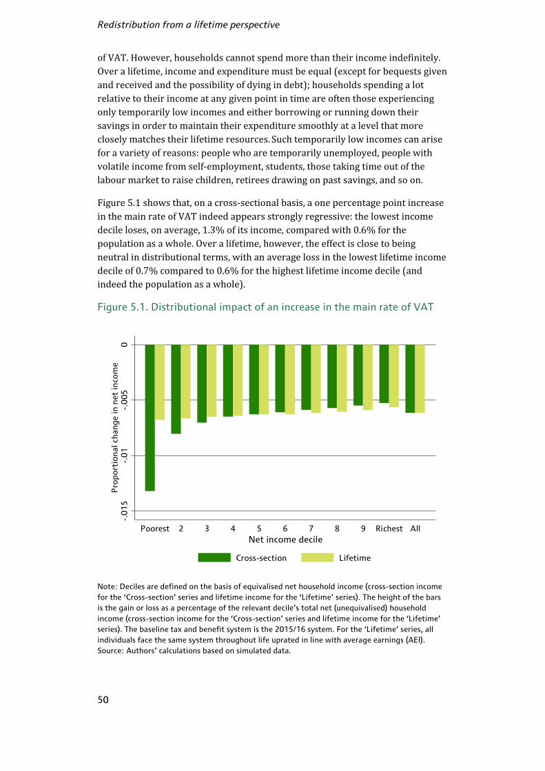
Redistribution from a lifetime perspective
50
of VAT. However, households cannot spend more than their income indefinitely. Over a lifetime, income and expenditure must be equal (except for bequests given and received and the possibility of dying in debt); households spending a lot relative to their income at any given point in time are often those experiencing only temporarily low incomes and either borrowing or running down their savings in order to maintain their expenditure smoothly at a level that more closely matches their lifetime resources. Such temporarily low incomes can arise for a variety of reasons: people who are temporarily unemployed, people with volatile income from self-employment, students, those taking time out of the labour market to raise children, retirees drawing on past savings, and so on. Figure 5.1 shows that, on a cross-sectional basis, a one percentage point increase in the main rate of VAT indeed appears strongly regressive: the lowest income decile loses, on average, 1.3% of its income, compared with 0.6% for the population as a whole. Over a lifetime, however, the effect is close to being neutral in distributional terms, with an average loss in the lowest lifetime income decile of 0.7% compared to 0.6% for the highest lifetime income decile (and indeed the population as a whole). Figure 5.1. Distributional impact of an increase in the main rate of VAT
Note: Deciles are defined on the basis of equivalised net household income (cross-section income
for the ‘Cross-section’ series and lifetime income for the ‘Lifetime’ series). The height of the bars
is the gain or loss as a percentage of the relevant decile’s total net (unequivalised) household
income (cross-section income for the ‘Cross-section’ series and lifetime income for the ‘Lifetime’
series). The baseline tax and benefit system is the 2015/16 system. For the ‘Lifetime’ series, all
individuals face the same system throughout life uprated in line with average earnings (AEI).
Source: Authors’ calculations based on simulated data.
-.0
15
-.0
1-.
00
50
Pro
po
rtio
nal
cha
ng
e i
n n
et
inco
me
Poorest 2 3 4 5 6 7 8 9 Richest All
Net income decile
Cross-section Lifetime

Distributional effects of hypothetical tax and benefit reforms
51
The above results arise because items that are zero- or reduced-rated for VAT – and therefore not affected by a rise in the main rate – take up a larger share of the budgets of poorer households. Over a lifetime, we would expect richer households to devote a larger share of their resources to goods subject to VAT at the main rate and therefore to lose more from such a VAT increase than poorer households.22 However, this abstracts from the possibility of bequests: we find that the ratio of lifetime consumption to income is lower for the lifetime rich than the lifetime poor. This is consistent with the lifetime rich consuming a smaller share of their lifetime income than the lifetime poor, and leaving proportionally larger bequests. To the extent that this is true, it will mean that, although richer households consume proportionally more standard-rated goods, they will incur slightly smaller losses from an increase in the main rate of VAT. One consequence of raising the main rate of VAT is that it would increase the distortion towards producing and consuming zero- and reduced-rated goods and services instead of standard-rated ones. Such a distortion could be alleviated by extending the scope of VAT to cover those items that are currently zero-rated. Food is by far the biggest of these: the zero-rating of (most) food cost the government £17.5 billion in 2014–15.23 Likewise, increasing the VAT rate on those items that are currently taxed at the lower 5% rate (principally domestic fuel and power) towards the standard rate would reduce the distortion to households’ spending patterns. In addition to these efficiency gains, moving towards a more uniform VAT regime would simplify the system, eliminating peculiar quirks such as the main VAT rate treatment of chocolate-covered biscuits but not chocolate-covered cakes.24 Figure 5.2 shows the distributional impact of extending the main VAT rate to most zero- and reduced-rated goods.25 Levying or increasing VAT on those goods currently zero- or reduced-rated would be unambiguously regressive: on a cross-sectional basis, the average loss is 12.0% of income for the lowest income decile compared with 2.9% for the highest income decile, while over the lifetime the corresponding figures are 6.4% and 3.7%. This is because poorer households typically devote a larger share of their budgets to these items, and therefore will lose proportionally more from such a tax rise. However, Mirrlees et al. (2011) argue on efficiency grounds for such a reform and demonstrate that it is possible to design a set of direct tax cuts and benefit increases such that the overall package (including the flat-rate VAT) is revenue neutral, broadly distributionally neutral and would avoid worsening work incentives. 22
For more analysis of VAT payments by income and expenditure and their relationship to lifetime resources,
see Adam, Phillips and Smith (2011).
23 See https://www.gov.uk/government/statistics/main-tax-expenditures-and-structural-reliefs.
24 See http://www.hmrc.gov.uk/manuals/vfoodmanual/vfood6260.htm.
25 For a full list of zero- and reduced-rated goods, see Table 10.1 in Adam and Roantree (2015). Note that we
do not consider extending the standard rate of VAT to new houses, the portion of international passenger transport that takes place in the UK, and ships and aircraft above a certain size.

Redistribution from a lifetime perspective
52
Figure 5.2. Distributional impact of extending the main rate of VAT to
zero- and reduced-rated goods
Note: Deciles are defined on the basis of equivalised net household income (cross-section income
for the ‘Cross-section’ series and lifetime income for the ‘Lifetime’ series). The height of the bars
is the gain or loss as a percentage of the relevant decile’s total net (unequivalised) household
income (cross-section income for the ‘Cross-section’ series and lifetime income for the ‘Lifetime’
series). The baseline tax and benefit system is the 2015/16 system. For the ‘Lifetime’ series, all
individuals face the same system throughout life uprated in line with average earnings (AEI).
Source: Authors’ calculations based on simulated data.
5.3 What is the most effective way of redistributing
resources to the lifetime poor: out-of-work benefits,
in-work benefits or tax cuts? In principle, policymakers might be interested in designing policies that redistribute towards the lifetime poor. In this subsection, we consider how effective a number of alternative policies are at targeting the lifetime poor, and we contrast this with their cross-sectional impacts. The alternatives we consider are three measures with similar cross-sectional revenue consequences (around £3 billion per year), namely: (i) an increase in out-of-work benefits – a 16.5% increase in maximum income support, (income-based) jobseeker’s allowance, pension credit and (non-contributory) employment support allowance; (ii) an increase in in-work (i.e. work-contingent) benefits – an 18% increase in maximum working tax credit; (iii) an income tax cut – a 4% increase in the income tax personal allowance.
-.1
5-.
1-.
05
0P
rop
ort
ion
al
cha
ng
e i
n n
et
inco
me
Poorest 2 3 4 5 6 7 8 9 Richest All
Net income decile
Cross-section Lifetime

Distributional effects of hypothetical tax and benefit reforms
53
In addition, we also refer to VAT and income tax rate changes analysed in Sections 5.2 and 5.4. These do not have the same revenue implications, but we can still draw inferences about the cross-sectional and lifetime distributional implications. Obviously, there are many other policy reforms we could have considered, but these have been chosen as indicative of the types of policies that are often considered in policy debates around this issue. Figure 5.3 shows the cross-sectional effect of the three reforms listed above. Unsurprisingly, the most progressive reform is the increase to out-of-work benefits: gains are concentrated in the bottom two income deciles, with the largest average gain experienced by the lowest income decile (5.0%), in which there is a high share of non-working individuals (see Figure 2.4). Next most progressive is the increase to working tax credit. Here, the bottom four deciles are gainers, with gains peaking at an average of 1.7% in decile two. The bottom decile gains by less because fewer individuals here are entitled to working tax credit (because they are not working). The least progressive (indeed a regressive) reform is the income tax cut in the form of an increase in the personal allowance. Gains are concentrated among the upper half of the income distribution, reflecting the fact that the poorest adults have income that is too low to benefit from the giveaway, while dual-income couples – who tend to have higher family incomes – can benefit twice over. Figure 5.1 allows us to infer the cross-sectional pattern of gains from a cut to the main rate of VAT. This would benefit all deciles, but the greatest gain in proportional terms would be for the bottom decile. This is because low-income households typically spend a lot relative to their income, and therefore pay a lot of VAT. Likewise, we can infer from Figure 5.6 that the cross-sectional distributional impact of a cut to the basic rate of income tax would be similar to – but somewhat more regressive than – that of the personal allowance increase (in Figure 5.3). The reason why the cut in the basic rate is more regressive is that it benefits individuals more the higher up the basic rate band they are (unlike the personal allowance cut, which is a fixed cash gain for all who remain basic rate payers). Over the lifetime, the picture is somewhat different, as shown in Figure 5.4.26 In particular, increases in out-of-work and in-work benefits are strongly progressive, with almost identical distributional patterns, while the income tax cut (personal allowance increase) is close to distributionally neutral. As already discussed, Figure 5.1 shows that the cut to the main rate of VAT is also close to distributionally neutral, while a cut to the basic rate of income tax remains regressive (Figure 5.6). 26
To aid comparison, we have scaled gains proportionally such that the ‘All’ bars are the same across reforms.
Without scaling, the reason why the ‘All’ bars are slightly different over the lifetime when they are the same in the cross-section (Figure 5.3) is that they depend on the timing of gains and losses over life (unlike in the cross-section).

Redistribution from a lifetime perspective
54
Figure 5.3. Cross-sectional distributional impact of increases to out-of-
work and in-work benefits and of the income tax personal allowance
Note: Deciles are defined on the basis of cross-sectional equivalised net household income. The
height of the bars is the gain or loss as a percentage of the relevant decile’s total net
(unequivalised) household income. The ‘Out-of-work benefits’ series shows the effect of a 16.5%
increase in maximum income support, (income-based) jobseeker’s allowance and (non-
contributory) employment support allowance. The ‘In-work benefits’ series shows the effect of an
18% increase in maximum working tax credit. The ‘Income tax’ series shows the effect of a 4%
increase in the income tax personal allowance. In all cases, the baseline tax and benefit system is
the 2015/16 system.
Source: Authors’ calculations based on simulated data. What is most interesting here is the fact that increases in out-of-work and in-work benefits have such a similar distributional pattern. This is because, while the poorest individuals in the cross-section are often out of work, this is often a temporary state and many of the poorest individuals in a lifetime sense are in work some of the time and out of work some of the time (see Figure 2.4). In addition, when in work, they are relatively likely to be in low-paid work and therefore qualify for in-work support. Thus, it is possible to reach many of the lifetime poor through either out-of-work or in-work benefits. An advantage of increasing in-work benefits rather than out-of-work benefits is that they will – in general – have much less of a negative impact on work incentives: out-of-work benefits reduce the net-financial gain to being in work, while in-work benefits in the UK are contingent on working a certain number of hours. Thus, policymakers looking to target the lifetime poor might favour doing so through in-work benefits. The disadvantage of such an approach is that it would do less to help the lifetime poor in the particular periods that they were
0.0
1.0
2.0
3.0
4.0
5P
rop
ort
ion
al ch
an
ge
in
ne
t in
com
e
Poorest 2 3 4 5 6 7 8 9 Richest All
Net income decile
Out-of-work benefits In-work benefits Income tax

Distributional effects of hypothetical tax and benefit reforms
55
Figure 5.4. Lifetime distributional impact of increases to out-of-work and
in-work benefits and of the income tax personal allowance
Note: Deciles are defined on the basis of cross-sectional equivalised net household income. The
height of the bars is the gain or loss as a percentage of the relevant decile’s total net
(unequivalised) household income. The ‘Out-of-work benefits’ series shows the effect of a 16.5%
increase in maximum income support, (income-based) jobseeker’s allowance and (non-
contributory) employment support allowance. The ‘In-work benefits’ series shows the effect of an
18% increase in maximum working tax credit. The ‘Income tax’ series shows the effect of a 4%
increase in the income tax personal allowance. In all cases, the baseline tax and benefit system is
the 2015/16 system. All individuals face the same system throughout life uprated in line with
average earnings (AEI). To aid comparison, we have scaled gains proportionally such that the ‘All’
bars are the same across reforms.
Source: Authors’ calculations based on simulated data. not working, which could matter if they did not have access to savings or borrowing facilities (see discussion in Introduction). It would also do less to help the minority of the lifetime poor who do experience sustained periods without work. That said, recent experience suggests that the lifetime poor among younger cohorts may increasingly have substantial amounts of work over their lives but low levels of earnings rather than long periods out of the labour market (for cross-sectional evidence, see Belfield et al., 2015). 5.4 How well do tax changes target the lifetime rich? In this subsection, we consider the distributional impact of changes to income tax rates. We focus on the higher rate of income tax but also discuss the basic rate for comparison. Ideally, we would also like to look at the additional (45p) rate of income tax that applies to incomes above £150,000, but our model is unlikely to capture incomes right at the top of the income distribution well enough for this to
0.0
02
.00
4.0
06
.00
8P
rop
ort
ion
al ch
an
ge
in
ne
t in
com
e
Poorest 2 3 4 5 6 7 8 9 Richest All
Net income decile
Out-of-work benefits In-work benefits Income tax

Redistribution from a lifetime perspective
56
be possible. As before, reforms are applied using the 2015/16 tax and benefit system as a base. Figure 5.5 shows the distributional impact of a one percentage point increase in the higher rate of income tax, from a cross-sectional and lifetime perspective. Our analysis here does not make any allowance for behavioural response. While we do not have much formal evidence on how responsive higher-rate taxpayers are to changes in the tax rate, it seems unlikely that they are very responsive since many are males and/or primary earners in families. HM Revenue and Customs (HMRC) estimates that such a reform would raise £1.3 billion per year from a cross-sectional perspective in 2016–17. The figure shows that the reform is extremely progressive in the cross-section: the bottom four deciles are completely unaffected (because these individuals do not earn enough to pay the higher rate), and it is only the top two deciles that experience a hit to incomes of more than 0.1%, with losses peaking at 0.38% for the top decile. Over the lifetime, the reform remains strongly progressive, but Figure 5.5. Distributional impact of a one percentage point increase in the
higher rate of income tax
Note: Deciles are defined on the basis of equivalised net household income (cross-section income
for the ‘Cross-section’ series and lifetime income for the ‘Lifetime’ series). The height of the bars
is the gain or loss as a percentage of the relevant decile’s total net (unequivalised) household
income (cross-section income for the ‘Cross-section’ series and lifetime income for the ‘Lifetime’
series). The baseline tax and benefit system is the 2015/16 system. For the ‘Lifetime’ series, all
individuals face the same system throughout life uprated in line with average earnings (AEI).
Source: Authors’ calculations based on simulated data. there is slightly more of an impact further down the distribution. Those in the top four deciles experience a loss exceeding 0.1% but, as before, it is the very top
0-.
00
2-.
00
4-.
00
6P
rop
ort
ion
al ch
an
ge
in
ne
t in
com
e
Poorest 2 3 4 5 6 7 8 9 Richest All
Net income decile
Cross-section Lifetime

Distributional effects of hypothetical tax and benefit reforms
57
decile that stands out, with a 0.26% fall. This reflects the greater persistence in earnings at the top of the distribution (i.e. highly paid individuals tend to remain highly paid) – see Figure 2.8 and Roantree and Shaw (2014). Thus, changes to the higher rate of income tax are reasonably effective at targeting the lifetime rich. For comparison, we also present the distributional impact of a one percentage point increase in the basic rate of income tax (Figure 5.6). This shows that the cross-sectional impact is progressive: the bottom decile is largely unaffected (because most individuals in this decile do not earn enough to pay income tax) and the average loss peaks at 0.60% for the ninth decile. The top decile loses by slightly less because a smaller share of income for these individuals is subject to the basic rate. Over the lifetime, the impact remains progressive, but much less so because many more individuals will pay basic rate income tax at some point in life than in any one year. The bottom decile suffers a loss of 0.34%, rising to 0.53% for the top decile. Figure 5.6. Distributional impact of a one percentage point increase in the
basic rate of income tax
Note: Deciles are defined on the basis of equivalised net household income (cross-section income
for the ‘Cross-section’ series and lifetime income for the ‘Lifetime’ series). The height of the bars
is the gain or loss as a percentage of the relevant decile’s total net (unequivalised) household
income (cross-section income for the ‘Cross-section’ series and lifetime income for the ‘Lifetime’
series). The baseline tax and benefit system is the 2015/16 system. For the ‘Lifetime’ series, all
individuals face the same system throughout life uprated in line with average earnings (AEI).
Source: Authors’ calculations based on simulated data.
-.0
06
-.0
04
-.0
02
0P
rop
ort
ion
al
cha
ng
e i
n n
et
inco
me
Poorest 2 3 4 5 6 7 8 9 Richest All
Net income decile
Cross-section Lifetime
Redistribution from a lifetime perspective
58
5.5 Summary In this section, we have considered various hypothetical tax and benefit reforms and investigated how distributional impacts differ when looking from a lifetime perspective rather than a cross-sectional perspective. Our main findings are as follows. To reduce inequality by the most, resources should be targeted towards working tax credit, income support, council tax benefit or child tax credit. These benefits cut inequality by substantially more than other benefits or tax cuts. This holds true from both a cross-sectional and a lifetime perspective, though the fall in inequality from a lifetime perspective is smaller. In the cross-section, increases in the main rate of VAT appear regressive, but not when looked at over the lifetime. This supports other analysis that has found that increasing the main rate of VAT does not appear regressive when losses are expressed as a proportion of expenditure. Increases to VAT on zero- and reduced-rated goods are mildly regressive from a lifetime perspective. This is because the lifetime poor spend a greater share of their income on zero- and reduced-rated goods. However, it would be possible to compensate poorer households for losses such that the overall reform is revenue neutral, broadly distributionally neutral and avoids worsening work incentives. In-work benefits are just as good at targeting the lifetime poor as out-of-work benefits but do so without worsening work incentives by nearly so much. As a result, policymakers looking to target the lifetime poor might favour doing so through in-work benefits. Increases in the higher rate of income tax do target the lifetime rich reasonably well, due to lower mobility at the top of the income distribution.

59
© Institute for Fiscal Studies
6. Policy conclusions
1. The lifetime impact of policies matters. A coherent evaluation of economic well-being should consider circumstances over the lifetime and not just at a single point in time. The reason is simple: individuals typically live for many years, and experience dramatic change in their circumstances over this time. In practice, however, data limitations mean that most analysis of the tax and benefit system is based on snapshot information about a single cross-section of people. For example, analysis of income inequality or the distributional impact of tax and benefit reforms has tended to look exclusively at current circumstances. A cross-sectional perspective might suffice if circumstances do not change too much across life, because then the snapshot is informative about longer-run outcomes. However, this is not the case: for example, in our simulations – which match patterns in real data well – individuals experience considerable change in family composition, employment, earnings, and so on across life (see Figures 2.1–2.7). As a consequence, analysis of the tax and benefit system from a lifetime perspective can look quite different to the equivalent analysis conducted on a cross-section. For example, in Section 3.4, we showed that the tax and benefit system is considerably less effective at reducing lifetime inequality than cross-sectional inequality. Likewise, in Section 4, we showed that historical tax and benefit reforms have affected lifetime inequality but not by as much as cross-sectional inequality. That is not to say that snapshot outcomes do not matter. A good reason why one might want to look at snapshot outcomes is if short-term hardship is particularly damaging to lifetime welfare. This might be the case if there are borrowing constraints or uncertainty, which mean that individuals are unable or unwilling to borrow to smooth out income fluctuations over time. Evidence – including in our own previous work (Roantree and Shaw, 2014) – suggests that borrowing constraints and uncertainty do matter, arguing in favour of continuing to consider snapshot outcomes. However, this is in addition to lifetime outcomes not instead of them. The government is starting to recognise the importance of taking a longer-run perspective when analysing policy impacts. For example, HM Treasury and HMRC have recently developed a lifetime simulation model (LINDA) that allows them to estimate the impact of tax and benefit reforms on longer-run outcomes. This model is currently being used internally to assess the lifetime distributional impact of policy proposals. Nevertheless, the vast majority of public policymaking is focused on the immediate rather than long-term effect of policies. Greater consideration of long-term outcomes would give a fuller picture of the effect of (for example) tax and benefit reforms and would provide a more comprehensive basis for analysing policy.

Redistribution from a lifetime perspective
60
2. Policymakers should be more explicit about their redistributive objectives: is a policy designed to alleviate short-run hardship or to reduce inequality in lifetime resources? In Section 2, we showed that the snapshot poor and lifetime poor are often not the same people. Individuals in the poorest lifetime decile spend, on average, less than a quarter of life in the poorest cross-sectional decile (Figure 2.8) and, while the snapshot poor are often out of work, the lifetime poor are, on average, in paid work for the majority of their working life (Figure 2.4). As a result of these differences, policies that alleviate short-run hardship may not target lifetime outcomes very well (and vice versa). Increases in out-of-work benefits help most those who are right at the bottom of the cross-sectional distribution (Figure 5.3) but the impact extends much further up the distribution over the lifecycle (Figure 5.4). Therefore, in order to assess whether a policy is achieving its distributional aims, it is important to know what exactly it is trying to achieve: alleviate short-run hardship or reduce lifetime inequality? Policymakers have not tended to be particularly explicit about their answer to this question, but have implicitly focused on short-run outcomes. For example, one of the stated advantages of WFTC was that ‘it could prove a highly effective way of targeting help at [presumably snapshot] low-income families, thus reducing poverty and strengthening the family.’27 However, as we have seen, the lifetime impact of such policies can differ substantially from the snapshot impact. Also, as the rationale for redistributing towards the cross-sectional poor is likely to be different to that for redistributing towards the lifetime poor (given the evidence we have presented in this report), the set of appropriate policy instruments one might consider is also likely to be different. 3. A binary distinction between working and non-working families is often not a particularly useful way to think about policy. Over recent years, there has often been a sharp distinction made in policy debates between working and non-working families, with the former sometimes deemed more worthy of support.28 However, this fails to take account of the rather more complex dynamics individuals face over the course of their lifetime: as we have seen, very few individuals are
27 HM Treasury (1997, p. 43), cited in House of Commons Library (1998).
28 See, for example, ‘David Cameron: Working parents to save £5,000 a year under Tory childcare pledge’, The
Telegraph, 14 April 2015, http://www.telegraph.co.uk/news/politics/david-cameron/11534665/David-Cameron-30-hours-of-free-childcare-a-week-for-working-parents.html; ‘Election 2015: 'I'll put working families first' - Ed Miliband’, BBC News web site, 6 May 2015, http://www.bbc.co.uk/news/election-2015-32603762; and ‘Working parents exasperated over large families on benefits, says Harman’, The Guardian, 7 April 2013, http://www.theguardian.com/politics/2013/apr/07/working-families-exasperated-benefits-harman.

Policy conclusions
61
permanently out of work (Figure 2.4); there is substantial variation in individual incomes over time (Figure 2.5); the poor are not always poor and, albeit to a lesser extent, the rich are not always rich (Figure 2.8). In addition, benefit entitlement is not restricted to the lifetime poor: on average, those in the richest lifetime decile spend almost one-fifth of their lifetime entitled to one of the main means-tested benefits (Figure 2.7). This highlights the importance of viewing the current circumstances of families as just one snapshot in a lifetime of many years, subject to considerable dynamics and variation. 4. Policymakers looking to target the lifetime rich can actually do so reasonably well using the higher rate of income tax. In Section 5.4, we showed that measures aimed at the cross-sectional rich, such as increases in the higher rate of income tax, do a reasonably good job of targeting the lifetime rich too (see Figure 5.5). This is in contrast with the reforms aimed at redistributing to the lifetime poor that we investigated (see Figure 5.4). An important reason for this is the differing degree of mobility in the two tails of the income distribution: in simple terms, rich individuals more often remain rich than poor individuals remain poor (see Figure 2.8). As a result, policymakers wishing to target the lifetime rich can do so reasonably effectively using the higher rate of income tax. We also looked at the progressivity of increases in the basic rate of income tax (Figure 5.6) and the income tax-free personal allowance (Figures 5.3 and 5.4) from a lifetime perspective. We found that the distributional impact of increasing the basic rate of income tax is much less progressive from a lifetime perspective than from a cross-sectional perspective. This is because many more individuals pay basic rate income tax at some point in life than in any one year, while increases in the personal allowance – regressive from a cross-sectional perspective – are broadly neutral from a lifetime perspective. The lifetime distributional impact of these measures is therefore more similar to increases in the main rate of VAT than to increases in the higher rate of income tax, something policymakers should bear in mind when assessing the consequences of broad-based tax changes. It would be interesting to understand how effective the additional rate of income tax (levied on incomes above £150,000) is at targeting the lifetime very rich. Unfortunately, our modelling framework does not capture individuals on the highest incomes sufficiently well enough to be able to answer this question. 5. Policymakers looking to target the lifetime poor might favour doing so through in-work rather than out-of-work benefits. In Section 5.3, we showed that, from a cross-sectional perspective, increasing maximum out-of-work benefit entitlement is considerably more progressive than increasing maximum in-work benefit entitlement (see Figure 5.3). Over

Redistribution from a lifetime perspective
62
the lifetime, however, the two are about as progressive as each other (Figure 5.4). This reason for this is that, while many of the cross-section poor are out of work, this is often a temporary state. Indeed, on average, those in the poorest lifetime decile spend the majority working life in paid work. In addition, when the lifetime poor are in work, they are relatively likely to be in low-paid work and therefore qualify for in-work support. As a result, it is possible to redistribute towards many of the lifetime poor either through out-of-work or through in-work benefits. The advantage of in-work benefits is that they will – in general – have a better impact on work incentives than out-of-work benefits: in-work benefits are contingent on working, so they do not discourage individuals from working nearly so much.29 Indeed, one of the aims of in-work benefits is to move individuals into paid work, and previous analysis (e.g. Brewer et al., 2006) has shown that they can be effective at doing this. If we were able to incorporate these behavioural responses into our analysis, we would find that in-work benefits do not just help existing low-income workers, but also encourage some to move into paid work. Thus, policymakers looking to target the lifetime poor might favour putting more emphasis on in-work benefits. The disadvantage of such an approach is that it would do less to help the lifetime poor in the particular periods that they were not working, which could matter if they did not have access to savings or borrowing facilities, and it would also do less to help the minority of the lifetime poor who do experience sustained periods without work. 6. Maintaining the current distortionary system of VAT is hard to justify on distributional grounds. The current system of VAT distorts production and consumption choices towards zero- and reduced-rated (5% tax rate) goods and services instead of standard-rated (20%) ones. This has welfare costs because it diverts choices away from the bundle of goods and services that individuals would otherwise prefer. It is therefore desirable to eliminate this distortion on efficiency grounds, as was argued by Mirrlees et al. (2011). A difficulty with removing zero and reduced rates in isolation is that it would be regressive. As Figure 5.2 shows, on a cross-sectional basis, the average loss is 12.0% of income for the bottom income decile compared with 2.9% for the top income decile. From the lifetime perspective, however, Figure 5.2 demonstrates that the impact would – while still regressive – be considerably less regressive than the cross-sectional impact: the losses at the bottom and top of the income distribution are 6.4% and 3.7%, respectively. Moreover, Mirrlees et al. (2011) demonstrate that it is possible to design a set of direct tax cuts and benefit increases such that the overall package
29 Depending on what form the work-conditionality takes, in-work benefits may still discourage work for
some individuals (e.g. second earners in couples).

Policy conclusions
63
(including the flat-rate VAT) is revenue neutral, broadly distributionally neutral and would avoid worsening work incentives. The case for maintaining the current distortionary system of VAT on distributional grounds is weaker still from a lifetime perspective. 7. The potential exists to achieve what the current tax and benefit system does more efficiently. Income taxes and means-tested benefits create a disincentive to work because they reduce the net return to working. This is often unavoidable given that taxes and benefits are income-related. However, as various authors have pointed out, this need not be the case with redistribution that is intrapersonal (i.e. across periods of life). The reason for this is that it may be possible to create an explicit link between taxes paid at one point in life and benefits received at another, such that taxes are no longer perceived as pure (distortionary) taxes but at least partly as ‘social insurance’ contributions (which are closer to enforced saving). This is something that has potentially been missed in the UK’s move away from a contributory system over recent decades. As described in Section 3.3, we find that more than half of the redistribution undertaken by the tax and benefit system is intrapersonal. This suggests considerable potential for creating such a benefit–contribution link. What form might such a benefit–contribution link take? One already alluded to is contributory benefits, whereby entitlement to certain benefits (such as unemployment insurance and sickness benefit) depends on past social insurance contributions. Another would be to replace certain benefits with loans to cover periods of short-run hardship (just as student loans have, over the last 25 years, replaced maintenance grants as the main way to support those in higher education). A somewhat more radical suggestion that builds on these two ideas is a system of welfare accounts, such as that proposed by Bovenberg, Hansen and Sørensen (2008). These work as follows. For individuals who are working, mandatory contributions are credited to their account. When individuals meet eligibility conditions for receipt of particular benefits, these are debited from the account. At retirement, account surpluses are returned to individuals, while deficits are written off. Having said all this, the case for linking contributions and benefit receipt is not clear cut. It relies crucially on individuals recognising and responding to the fact that contributions are not a tax but are closer to a form of enforced saving. It is by no means certain that this would happen, given that many people in the UK still think that National Insurance contributions fund state pensions and other contributory benefits (when in fact the link is almost non-existent). In addition, some reform proposals, such as the system of welfare accounts proposed by Bovenberg et al. (2008), imply a large giveaway (in this case at retirement, when surpluses are returned to individuals). For such a policy to be cost-neutral, it requires a substantial employment response: individuals understand that part of their tax payments actually reflects
Redistribution from a lifetime perspective
64
enforced saving from which they can subsequently benefit, and therefore decide to work more as a result. Whether – and on what scale – such a response would materialise is a topic on which there is currently little empirical evidence. These are important questions for future research, but they nevertheless raise the possibility that it may be possible for policymakers to achieve what the current tax and benefit system does more efficiently. 8. Targeting lifetime redistribution more effectively may require new policy instruments. None of analysis in this report suggests that the current tax and benefit system, assessed largely against contemporaneous circumstances, does especially well at redistributing resources towards lifetime poor. For example, as we saw in Section 3.4, the tax and benefit system is much less effective at reducing inequality over the lifetime than from a cross-sectional perspective: over the lifetime, it reduces the Gini coefficient by 14.9% compared to 31.4% in the cross-section. Similarly, results in Section 5.3 show that reforms targeting the cross-section poor, such as increases to out-of-work benefits, are much less focused on the lifetime poor. Greater redistribution, when considered on a lifetime basis, should be possible given how well the current tax and benefit system, based on snapshot circumstances, can target snapshot outcomes. What is likely to be required in order to target lifetime outcomes is taxes and benefits that condition on longer-run circumstances. What form might this take? This is again an important topic for future work, but it could include Vickrey’s (1947) idea of using lifetime earnings as a base for taxation or the suggestion by Laroque (2010) of a history-dependent tax and benefit scheme based around the idea of a social account that tracks an individual’s cumulative debts to, or claims on, other citizens. Both of these suggestions potentially incorporate a far greater degree of flexibility in the design of taxes and benefits based on lifetime information, and therefore would allow greater targeting of lifetime outcomes. One issue is the greater degree of complexity implied by the use of lifetime information. Any gains from using such information must be traded off against the costs of having a more complicated tax and benefit system that individuals may find difficult to understand. That notwithstanding, if policymakers are interested in lifetime outcomes – as we have argued they should be – there is at least a case for new tax and benefit instruments in order to achieve greater lifetime redistribution far more effectively.

65
© Institute for Fiscal Studies
References
Adam, S. and Browne, J. (2010), ‘Redistribution, work incentives and thirty years of UK tax and benefit reform’, Institute for Fiscal Studies (IFS), Working Paper no. W10/24 (http://www.ifs.org.uk/publications/5367). Adam, S., Phillips, D. and Smith, S., in consortium (2011), A Retrospective Evaluation of Elements of the EU VAT System: Full Report, Institute for Fiscal Studies (IFS), external publication commissioned by European Commission, TAXUD/2010/DE/328, available at http://ec.europa.eu/taxation_customs/resources/documents/common/publications/studies/report_evaluation_vat.pdf (http://www.ifs.org.uk/publications/5947). Adam, S. and Roantree, B. (2015), ‘Options for increasing tax’, in C. Emmerson, P. Johnson and R. Joyce (eds), IFS Green Budget 2015, Institute for Fiscal Studies (IFS) (http://www.ifs.org.uk/publications/7553). Barr, N. (2004), Economics of the Welfare State, Oxford: Oxford University Press. Belfield, C., Cribb, J., Hood, A. and Joyce, R. (2015), Living Standards, Poverty and Inequality in the UK: 2015, Institute for Fiscal Studies (IFS) Report no. R107 (http://www.ifs.org.uk/publications/7878). Blundell, R., Duncan A., McCrae, J. and Meghir, C. (2000), ‘The labour market impact of the working families’ tax credit’, Fiscal Studies, vol. 21, pp. 75–103. Bovenberg, A., Hansen, M. and Sørensen, P. (2008), ‘Individual savings accounts for social insurance: rationale and alternative designs’, International Tax and Public Finance, vol. 15, pp. 67–86. Bozio, A. Emmerson, C., O’Dea, C. and Tetlow, G. (2013), ‘Savings and wealth of the lifetime rich: evidence from the UK and US’, Institute for Fiscal Studies (IFS), Working Paper no. W13/30 (http://www.ifs.org.uk/publications/7020). Brewer, M., Duncan, A., Shephard, A. and Suárez, M. (2006), ‘Did working families' tax credit work? The impact of in-work support on labour supply in Great Britain’, Labour Economics, vol. 13, pp. 699–720. Brewer, M., Costa Dias, M. and Shaw, J. (2012), ‘Lifetime inequality and redistribution’, Institute for Fiscal Studies (IFS), Working Paper no. W12/23 (http://www.ifs.org.uk/publications/6551). Browne, J. and Elming, W. (2015), ‘The effect of the coalition’s tax and benefit changes on household incomes and work incentives’, Institute for Fiscal Studies (IFS), Briefing Note BN159 (http://www.ifs.org.uk/publications/7534).

Redistribution from a lifetime perspective
66
Bolton, P. (2014), ‘Education spending in the UK’, House of Commons Library, SN01078, available at http://researchbriefings.parliament.uk/ResearchBriefing/Summary/SN01078. Carpentier, V. (2004), Historical Statistics on the Funding and Development of the UK University System, 1920–2002 [computer file], Colchester, Essex: UK Data Archive [distributor], SN: 4971, http://dx.doi.org/10.5255/UKDA-SN-4971-1. Crawford, R. and Emmerson, C. (2012), NHS and Social Care Funding: The Outlook to 2021/22, Institute for Fiscal Studies (IFS) report, available at http://www.nuffieldtrust.org.uk/sites/files/nuffield/publication/120704_nhs-social-care-funding-outlook-2021-22_0.pdf. Department for Education and Employment (1998), Statistics of Education: Schools in England, London: The Stationery Office Department of Health (2011), Resource Allocation: Weighted Capitation Formula, DH Financial Planning and Allocations Division, available at https://www.gov.uk/government/uploads/system/uploads/attachment_data/file/216320/dh_124947.pdf . Department for Work and Pensions (DWP) (2015), Households Below Average Income: An Analysis of the Income Distribution 1994/95 to 2013/14, available at https://www.gov.uk/government/uploads/system/uploads/attachment_data/file/437246/households-below-average-income-1994-95-to-2013-14.pdf. Disney, R., Emmerson, C. and Tetlow, G. (2007), ‘What is a public sector pension worth’, Institute for Fiscal Studies (IFS) Working Paper no. W07/17 (http://www.ifs.org.uk/publications/4051). Dominitz, J. (1998), ‘Earnings expectations, revisions, and realizations’, Review of Economics and Statistics, vol. 80, pp. 374–388. HM Treasury (1997), ‘Employment Opportunity in a Changing Labour Market’, The Modernisation of Britain's Tax and Benefits System No. 1, p. 43. Hood, A. and Oakley, L. (2014), ‘A survey of the GB benefit system’, Institute for Fiscal Studies (IFS), Briefing Note BN13 (http://www.ifs.org.uk/publications/1718). Hood, A. and Phillips, D. (2015), ‘Benefit spending and reforms: the coalition government’s record’, Institute for Fiscal Studies (IFS), Briefing Note BN160 (http://www.ifs.org.uk/publications/7535). House of Commons Library (1998), Working Families Tax Credit and Family Credit, Research Paper 98/46. Laroque, G. (2010), ‘Commentary on means-testing and tax rates on earnings’, in J. Mirlees (ed), Dimensions of Tax Design, Oxford: Oxford University Press.

References
67
Lerman, R. and Yitzhaki, S. (1985), ‘Income inequality effects by income’, Review of Economics and Statistics, vol. 67, pp. 151–156. Levell, P. and Shaw, J. (2015), ‘Constructing full adult life-cycles from short panels’, Institute for Fiscal Studies (IFS), Working Paper W15/01 (http://www.ifs.org.uk/publications/7529). Manski, C. and Straub, J. (2000), ‘Worker perceptions of job insecurity in the mid-1990s: evidence from the Survey of Economic Expectations’, Journal of Human Resources, vol. 35, pp. 447–479. Mirrlees, J., Adam, S., Besley, T., Blundell, R., Bond, S., Chote, R., Gammie, M., Johnson, P., Myles, G. and Poterba, J. (eds) (2011), Tax by Design: The Mirrlees Review, Oxford: Oxford University Press for Institute for Fiscal Studies. Office of Health Economics (2012), Expenditure Data, Office of Health Economics, available at http://www.ohe.org/page/health-statistics/access-the-data/expenditure/data.cfm. Office for National Statistics (ONS) (2015), The Effects of Taxes and Benefits on Household Income, Financial Year Ending 2014, Office for National Statistics, available at http://www.ons.gov.uk/ons/rel/household-income/the-effects-of-taxes-and-benefits-on-household-income/2013-2014/etb-stats-bulletin-2013-14.html. Roantree, B. and Shaw, J. (2014), The Case for Taking a Life-Cycle Perspective: Inequality, Redistribution, and Tax and Benefit Reforms, Institute for Fiscal Studies (IFS), Report R92 (http://www.ifs.org.uk/publications/7130). Sen, A. (1973), On Economic Inequality, Oxford: Clarendon Press. Sen, A. (1992), Inequality Re-examined, Oxford: Oxford University Press and Cambridge, MA: Harvard University Press. Vickrey, W. (1947), ‘Resource distribution patterns and the classification of families’, in E. Denison, S. Selma Goldsmith and M. Kuznets (eds), Studies in Income and Wealth, Chicago: National Bureau of Economic Research (NBER), pp. 266–297.

68
© Institute for Fiscal Studies
A. Methodology
In this appendix, we describe the methodology we have used to create simulated tax and benefit profiles across life for the baby-boom cohort. A.1 Overview of method To answer questions about the lifetime impact of the tax and benefit system, we need to have data on individuals throughout their lives. Unfortunately, no survey data set in the UK can provide a long enough time series, so instead we make use of simulation procedures. The approach we take is to simulate lifecycle profiles for the main determinants of taxes and benefits and then run these profiles through a tax and benefit calculator to calculate taxes and benefits. The main determinants of taxes and benefits that we model are:
mortality; family composition (fertility, partnering and separation); health/disability (entitlement to the main disability benefits); hours of work (not working, part-time or full-time); earnings; housing tenure (whether a renter) and rent; council tax band; private pension income; consumption. We abstract from other less important determinants of taxes and benefits. Our simulated profiles are designed to replicate the experiences of a particular birth cohort of individuals – those born in the years 1945–1954 (which we label ‘baby-boomers’). We chose this cohort primarily because we have cross-sectional data covering most of their working lives, which we can use to improve our simulations (see below for our method). The cohort is also an important one, whose members have just begun to retire. Although we focus on a single cohort, the patterns observed are likely to be indicative of what other cohorts have experienced (or will experience). The primary method we use to simulate lifecycle profiles is called dynamic microsimulation. This involves estimating transition probabilities between different states at consecutive ages, and then using these transition probabilities to simulate lifecycle outcomes a year at a time for a set of artificial individuals. In this appendix, we outline how we have implemented this approach; see Levell and Shaw (2015) for more details. Our approach comprises four stages: estimation, simulation, imputation and validation. We discuss these in turn.

A. Methodology
69
Estimation The first step in our process is to use survey data to estimate a set of transition probabilities for most of the main determinants of taxes and benefits listed above. These transition probabilities tell us the likelihood that an individual moves from one state to another between consecutive ages given their current characteristics. For example, we might work out the probability that an unemployed person finds full-time work or the probability that a single person finds a partner. Ideally, we would like to estimate transition probabilities using only data for the baby-boom cohort. However, this would require a long-panel data set dating back to the 1960s, which is not available for the UK. The best data we have that follow individuals annually over time is the BHPS. This covers the period 1991–2008, meaning that we only observe the baby-boom cohort aged between their late 30s and early 60s. For transitions outside these ages, we have to rely on data from younger and older cohorts, whose experiences might not be exactly the same as the baby-boomers. To correct for biases that this might introduce, we adjust our transition probabilities so that aggregates match those for the baby-boomers, as observed in the LCFS and its predecessors (all of which we refer to as the LCFS in what follows). For example, we adjust transition probabilities in and out of work to match the aggregate employment rate of baby-boomers at each age. Simulation We begin with a set of starting values at age 16 for the key determinants of taxes and benefits for our cohort of interest. In addition, we use the LCFS and BHPS to draw values for sex and education (which are assumed to be fixed throughout life but are important for simulating other outcomes). We then draw transitions for each outcome for each individual to determine what state they experience in the next year. The likelihood of different transitions depends on the individual’s current circumstances. Once all variables have been determined for all individuals in the current year, we then move on to simulate outcomes in the following year, and so on to the end of life. Imputation We do not estimate transition probabilities for all variables. The actual values of earnings and rents, spending (used to calculate VAT and excise duties) and private pensions are imputed to individuals once the simulation stage is complete. Finally, taxes and benefits are calculated based on all the other variables, taking simulated behaviour as given (see below for more on our assumption of no behavioural response). Earnings and rents Two of the key monetary outcomes we simulate are earnings and rents. When microsimulating transitions in earnings and rents, we model ranks (the position in the distribution, e.g. the 75th percentile) rather than levels (e.g. £400 per

Redistribution from a lifetime perspective
70
week). We then impute levels using cross-sectional LCFS data for the relevant age and cohort. The reason for doing this is to allow for arbitrary differences in earning and rent levels across cohorts. Our transition probabilities are partly based on cohorts other than the baby-boomers, who might have experienced quite different earning and rent levels. If we were to model levels directly, then our simulations might not accurately reflect the experiences of the baby-boom cohort. By imputing levels from cross-sectional data for the relevant age and cohort, we ensure that our simulations match both the average earnings of the cohort of interest and the degree of inequality across individuals at each age. For ages where cross-sectional LCFS data are not available (at the start and end of working life), we project distributions backward using historical rates of earnings and rent growth and forward using earnings and rent forecasts.30 One important caveat is that most survey data (including the LCFS) understate incomes at the top of the distribution. We have not been able to do anything to correct for this here. This will affect a number of our results, implying, for example, that we will tend to underestimate the taxes paid by the richest individuals and to understate the degree of inequality. Spending Ideally, we would like to use the same approach for spending as we do for earnings and rents. Unfortunately, this is not possible because there is no UK data set that tracks individuals over time and includes detailed measures of consumption spending. We therefore impute average consumption spending to individuals based on their current age, income and family characteristics (independently of what happened to them in the past) based on cross-sectional LCFS data.31 This is done separately for spending categories with different tax treatments. For example, we separately impute spending on goods and services subject to standard, reduced and zero-rate VAT, and also spending on alcohol and tobacco, which are subject to excise taxes, and motor fuel. We do not impose that lifetime spending and lifetime income are equal. A more comprehensive analysis would explicitly model spending decisions and bequests given the resources individuals have available, but this is beyond the scope of the current project. Private pensions Our approach to private pension income is quite different to that for earnings. The reason is that we have access to projected private pension income profiles for exactly our cohort of interest for different possible retirement dates. These are derived using information from the ELSA about private pension wealth in 30
Medium term earnings forecasts are taken from the OBR’s Economic and Fiscal Outlook. For later years, we
assume earnings growth of 2%. We assume future rent growth of 3.0% a year (roughly equal to its average over the 20 years 1994–2014).
31 In cross-sectional simulation, it is common to add an error term in order to preserve the spread of the
distribution of spending. The reason we do not do this is because, without a data set that tracks individual spending patterns over time in the UK, we cannot capture the correlation in spending over time.

A. Methodology
71
2008.32 This gives us the opportunity to attach real-world pension income profiles to our simulated individuals. To make use of these profiles, we need a realistic way of assigning them to individuals, given employment and earnings histories and other characteristics. For example, an individual who has never worked is highly unlikely to receive a large pension. The problem with the ELSA profiles that we have access to is that they only contain contemporaneous (2008) information about individuals, not employment and earnings histories. This means that it is hard to do a good job assigning profiles to individuals using just these data. What we do instead is to use BHPS estimates of pension wealth in 2001 in an intermediate step.33 We run a regression in the BHPS data that relates pension wealth to contemporaneous and past characteristics (such as being continuously employed over the previous five years). Using this, we predict in our simulations which individuals will receive a private pension and, for those that do, their predicted rank in the pension wealth distribution in 2001. We then assign an ELSA pension profile to each individual with a private pension, assuming that individuals stay at the same rank in the pension wealth distribution between 2001 and 2008 (the date of the ELSA pension profiles).34 Taxes and benefits Given lifecycle profiles for the main determinants of taxes and benefits, we can now calculate individuals’ tax liabilities and benefit entitlements under different (counterfactual) tax and benefit systems (we consider systems between the 1978/79 system and the 2016/17 system). We do this by running individuals through IFS’s tax and benefit calculator, TAXBEN. We assume that individuals face the same tax system throughout life and hold behaviour fixed under the different systems (see discussion below for more details). Validation The steps above provide us with a set of individual lifecycle profiles for taxes and benefits and their main determinants for the baby-boom cohort from age 16 until death. In Levell and Shaw (2015), we report an extensive set of validation exercises, finding find that our simulations do well at replicating the experiences of the baby-boom cohort. We fit cross-sectional distributions (e.g. the employment rate and earnings distribution at each age) extremely well – partly a consequence of the way we have adjusted profiles using the LCFS data. We also do a good job of capturing transitions across ages, though there is some evidence 32
The authors are grateful to Rowena Crawford and Gemma Tetlow for providing us with these projected
private pension profiles.
33 These estimates of BHPS pension wealth were calculated for Disney et al. (2007).
34 We do not use the BHPS data alone (rather than the BHPS and ELSA data in combination) because the BHPS
data (i) are not just for the baby-boom cohort, (ii) are for 2001, which is some way before retirement for most individuals in our cohort, and (iii) provide estimates of pension wealth rather than pension income streams, as in the ELSA data.
Redistribution from a lifetime perspective
72
that we slightly understate the persistence of some outcomes over long horizons (e.g. earnings 10 years ahead given earnings today). A.2 Key assumptions It is a highly complex task to model taxes and benefits and their effects on individuals over the lifecycle, and our analysis therefore necessarily makes a number of important assumptions. Here we discuss these. Time periods As already mentioned, we focus on the baby-boom cohort, which we define to be individuals born 1945–54. Although we focus on a single cohort, we expect that the patterns observed will be indicative of what other cohorts have experienced (or will experience). It is hard to be precise about this as we do not have data on full lifecycles for other cohorts with which to draw comparison, but patterns of family composition, employment and earnings, etc., over the lifecycle tend to be broadly similar across cohorts. We simulate 5,000 individuals between age 16 and the end of life. We model individuals on an annual basis but, given the data we use, this is really a sequence of annual snapshots rather than a sequence of year-long observations. This means that we will miss within-year transitions (such as short spells of unemployment) that occur between the annual snapshots. Unit of analysis We undertake analysis at the individual level, because we can follow individuals over time (unlike families, which change due to births, deaths, partnering and separation). We assume that there is equal sharing of resources within couples. For analysis concerning resource transfers (Sections 3.1–3.3), this means that earnings, taxes and benefits for each individual in a couple are calculated by dividing family-level values by two. For analysis about inequality of living standards (Section 3.4 onwards), family earnings, taxes and benefits are equivalised using the modified OECD equivalence scale and assigned to individuals. For lifetime variables, we equivalise annual values and then sum across life. Discount rates Lifetime variables (e.g. lifetime earnings) are calculated as the 2015/16 net present value (NPV) of the corresponding annual variables, where the discount rate used is the interest rate on government borrowing (based on consol yields taken from the Debt Management Office).35 We use this rate because it represents 35 The ‘2½% Consolidated Stock Average Yields’ are taken from
http://www.dmo.gov.uk/index.aspx?page=Gilts/Yields. A rate of 5.25% is assumed for yields after 2014 (the
20-year average for the period 1994–2014).

A. Methodology
73
the rate at which the government can trade off resources over time. This means that resources received or relinquished earlier are more valuable than those received or relinquished later. We show the sensitivity of some of our results to the assumed discount rate in Appendix D. Synthetic cross-section Many of our results compare lifetime outcomes with those for the cross-section. As stated above, the lifecycles we simulate are for the baby-boom cohort – those born in the years 1945–1954. The question is, what cross-section should we compare these to? One possibility is to use the actual LCFS cross-section for a given year (e.g. the most recent year of data uprated to 2015/16). This has the advantage that it uses the same data as might be used for a standard cross-sectional analysis. The disadvantage is that it combines lots of cohorts, so differences relative to the simulated lifecycles might be due to cohort effects rather than the switch to a lifecycle perspective. Because of this disadvantage, we use a second alternative, which is to construct a synthetic 2015/16 cross-section based on our simulated lifecycles for the baby-boom cohort. We do this by uprating financial variables (earnings, consumption and rent) to 2015/16 using average earnings growth (or a projection thereof for future values) and then treating all observations for the baby-boom cohort across different ages as though they were realised in 2015/16.36,37 This creates a cross-section for the baby-boom cohort: it describes what the 2015/16 population would look like if all cohorts were the same as the baby-boom cohort. As a result, any differences relative to the lifetime will be due to the lifetime perspective rather than the cohorts under consideration. In Appendix F, we examine how close our synthetic cross-section is to the 1978 and 2012 LCFS cross-sections. While there are some differences, the synthetic and real-world cross-sections are broadly consistent, and it turns out that results using the different approaches tell a similar story. Assumptions regarding the tax and benefit system
Taxes and benefits modelled We model most major personal taxes and benefits over the period we consider (1978/79 to 2016/17). The taxes we model are: income tax, employee National Insurance, council tax, community charge, domestic rates, VAT and alcohol, tobacco and fuel duties. The benefits we model are: income support/jobseeker’s allowance, housing benefit, council tax benefit, community charge benefit, 36
The reason we do not uprate rent in line with rents is because there is no rental price index going far enough
back in time.
37 Things are a bit more complicated for pension entitlements because they depend on past earnings. For
these, we take the pension entitlements accrued by our simulated individuals under the 2015/16 tax and benefit system and uprate or downrate them according to average earnings growth in order to put them in 2015 values.

Redistribution from a lifetime perspective
74
domestic rates rebates, family credit, working families’ tax credit, working tax credit, child tax credit, child benefit, one parent benefit, maternity grant, the state pension (both basic and earnings-related), the winter fuel payment, employment and support allowance, incapacity benefit, invalidity benefit, disability living allowance, attendance allowance and mobility allowance. The only contributory benefit (i.e. benefit where receipt depends on past contributions) that we model is the state pension. For this, we implement all the main contribution rules under current and historic systems. We abstract from contribution conditions in other benefits, such as (contribution-based) jobseeker’s allowance and incapacity benefit. Not all taxes and benefits are present in all years over the period we consider. We calculate those taxes and benefits appropriate to the system under consideration. We do not model ‘business taxes’ such as corporation tax and business rates because they are very difficult to attribute to individuals. We also do not model employer National Insurance because it is hard to model satisfactorily in TAXBEN. We also do not model capital taxes such as inheritance tax, stamp duties and capital gains tax. We ignore tax on savings income (and the implications of savings income for tax credit entitlement) and also tax relief on individual pension contributions.38 Benefit take-up We assume full take-up of benefits: all those who are eligible to receive a certain benefit claim it. In practice, take-up of means-tested benefits is often considerably less than 100%.39 Thus, our analysis measures the effect of benefit entitlement rather than benefit receipt. Behavioural responses For simplicity, we assume that there are no behavioural responses to tax and benefit changes: employment, gross earnings, spending and other determinants of taxes and benefits remain unchanged when individuals are exposed to different tax and benefit systems. This is a strong assumption, particularly when there are large differences between the actual tax and benefit systems that individuals experienced and the counterfactual system. This will be the case, for example, when we expose individuals from the 1970s to the current tax and benefit system because there has been a dramatic fall in top marginal income tax rates (among other things). Ideally, we would like to relax the assumption of no behavioural responses, but this would require an extremely complicated model of behaviour that is beyond the scope of the project. 38
The reason for this is that we do not model savings or pension contributions directly due to data limitations
and the complexity in modelling them satisfactorily. Employer pension contributions are not included in our wage data, and so are (correctly) left untaxed in our simulations.
39 See
https://www.gov.uk/government/uploads/system/uploads/attachment_data/file/222914/tkup_first_release_0910.pdf.

A. Methodology
75
Contracting out Individuals making contributions to recognised private pension schemes were able to opt out of the state second pension (SSP; formerly State Earnings-Related Pension Scheme, SERPS) and pay a lower rate of National Insurance Contributions until 2012 (2016 for members of defined benefit pension schemes).40 This was known as ‘contracting out’. Ideally, we would model this decision and calculate state and private pensions appropriately. Unfortunately, this is not feasible as we do not observe changes in individuals’ private pension arrangements at an appropriate frequency. Instead, we assume that any individual with positive private pension income in retirement was contracted out for the entirety of their life and does not receive any SSP/SERPS income: this is reasonable as most individuals with private pensions were indeed contracted out, but it does mean that we slightly understate the SSP/SERPS entitlement of some individuals. Because individuals can only opt out of the state earnings-related pension if they are contributing to a recognised private pension scheme, one could argue that some of this private pension (the part that replaces state provision) should be counted as part of the tax and benefit system. In this case, a fraction of private pension contributions would be treated as tax and a fraction of private pension income received would be treated as benefits. Alternatively, one could argue that, because the private pension is provided by the private sector, it should not be counted as part of the tax and benefit system. For simplicity, we take the latter approach, but bear in mind that this will affect our estimates of the impact of the tax and benefit system. For example, it will affect the degree to which the tax and benefit system is seen to redistribute across periods of life (as that is a large part of what an earnings-related pension achieves). Local taxes Local taxes vary by location and (roughly) by house value. Assigning exact values for such taxes to households is therefore difficult. Thus, we make a few simplifying assumptions. The system of local taxation underwent two substantial changes over our period. Initially, a system of domestic rates was in place. This was replaced in England and Wales in 1990 by the community charge or ‘poll tax’ (the reform had taken place in Scotland in the previous year). The community charge was then replaced by the current system of council tax in 1993. Northern Ireland retained the system of domestic rates throughout this period. In our analysis, we calculate local taxes assuming that all households face the systems that operated in England. Council tax liability depends which house value band, A–H, the family’s house falls into (based on 1991 property values). Local authorities are allowed to set 40
In practice, many occupational (particularly defined benefit) pension schemes required members to contract
out.

Redistribution from a lifetime perspective
76
their own band D rate but must charge other bands in fixed proportions relative to the band D rate. In our simulations, we model council tax band but not the variation across local authorities in the band D rate, instead setting it equal to the national average in each year. Community charge was a flat-rate tax per adult that varied across local authorities. As with council tax, we abstract from this local authority variation, instead assuming that all individuals are charged the national average rate. Domestic rates depended on (unbanded) house values. Rather than model house values directly, we assume a house value equal to the mid-point of the current council tax band. We then multiply these by the average domestic rate ‘poundage’ in each tax year. The resulting numbers are then scaled each year such that the average rate payment is equal to that for our cohort as observed in the LCFS. Assets tests Means-tested benefits and some (historic) tax credits involve an assets test whereby entitlement is reduced for individuals with savings above a certain level and removed altogether above a higher level. For example, under the 2015/16 tax and benefit system, the income support award a working-age family receives is reduced if the family has savings above £6,000 and completely eliminated above £16,000. We ignore these assets tests as we do not model savings. This means we will overstate entitlement to benefits and tax credits, particularly for older individuals who have accumulated more savings. This is likely to have a systematic (but small) effect on our results. For example, we may overstate the amount of redistribution that is across periods of life (Section 3.3) because we overestimate benefit entitlements for high-wealth individuals who are likely to have high lifetime tax payments. Note, however, that only a limited range of assets are counted, primarily liquid savings. Importantly, the family home, unannuitised wealth in private pensions and personal possessions are excluded. This will reduce substantially the number of families affected. Disability benefits The disability benefits we model are employment and support allowance (and its predecessors – incapacity benefit and invalidity benefit) and disability living allowance (and its predecessors – attendance allowance and mobility allowance). We estimate transition probabilities into and out of receipt using the BHPS. In reality, the amount of incapacity benefit and disability living allowance received depends on the nature and severity of the recipient’s condition. Rather than attempt to model the various entitlement categories, we assign typical values for each benefit. In particular, for incapacity benefit, we assign the long-term rate to all claimants in our simulations (because the vast majority receive this rate). For disability living allowance, we assign the higher rate of rate of mobility component plus the lower rate of the care component.41 We assume that individuals entitled to incapacity benefit would have been entitled to the 41 In 2014–15, the higher rate of rate of mobility allowance plus the lower rate of care allowance was worth
£74 per week. This is very close to the average value of disability living allowance given claimant counts and
rates provided in Hood and Oakley (2014) (£78).

A. Methodology
77
invalidity benefit prior to 1995 and to employment and support allowance from 2008 onwards.42 All recipients of invalidity benefit are assumed to receive the medium rate. All recipients of employment and support allowance are assumed to be in the support group of claimants. We assume that individuals entitled to disability living allowance would have been entitled to mobility allowance and the lower rate of attendance allowance before 1992. Public service spending For most of our analysis, we do not try to attribute the benefits of public service spending back to individuals. Were we able to do this, it would give a more complete picture of what redistribution the government achieves, considering that the benefits of public services are not equally distributed. The difficulty is that we do not have good enough data to work out who benefits from public services and by how much. In effect, our main analysis is looking at half the story: redistribution performed by the tax and benefit system. The other half of the story – redistribution through public services – we leave for future work (and for a time when better data are available). In Appendix E, we do, however, present some analysis that includes health and education spending, attributed on a cost basis (rather than trying to value the benefits from such spending). Uprating In our analysis, we assume that the same tax and benefit system is in place throughout life. We do this because we are primarily interested in the characteristics of given tax and benefit systems from a lifetime perspective rather than, say, the experiences of a particular cohort under the systems they were actually exposed to. The latter is interesting but is not the focus of this report. In order to apply a given tax and benefit system to data from earlier or later years, we need to decide how to deal with the fact that financial variables (earnings, pensions, rents, etc.) tend to grow over time. A naive approach would be to ignore the issue and to use the same nominal tax and benefit thresholds in every year. The problem with this is that secular earnings growth would tend to mean that more people are subject to higher tax rates, fewer people are entitled to means-tested benefits and the real value of benefit payments falls. As a result, the government would see larger and larger surpluses over time. This scenario is patently absurd. Instead, what we need to do is define a normal ‘no reform’ level of uprating that describes how nominal tax and benefit parameters should be increased from year to year in order to count as the same tax system. We considered two alternatives: uprating in line with prices (the RPI) and uprating in line with earnings (the average earnings index, AEI). The former is closer to the actual default uprating rules used by the government, while the latter is closer to ensuring that the tax and benefit system raises the same revenue each year. We consider the second of 42
One of the aims of the incapacity benefit reform was to reduce the number of claimants, so our approach is
likely to understate the number of individuals who would have been entitled to invalidity benefit.

Redistribution from a lifetime perspective
78
these to be more appropriate, and so use this assumption throughout the main body of our report. Much of our analysis has been repeated using RPI uprating. We report the main results from this in Appendix C. We find that the two analyses tell largely the same story about the impact of the 2015/16 tax and benefit system. A third alternative uprating scheme would use the government’s actual default uprating rules that describe how every threshold will change from year to year in the absence of explicit policy announcements. We choose not to do this because, over long periods of time, this can lead thresholds that are uprated differently to cross in unrealistic ways.

79
© Institute for Fiscal Studies
B. Intrapersonal redistribution
In this appendix, we derive a formula for the share of redistribution that is intrapersonal. Let denote benefits received, taxes paid and = − − redistribution, where is the no-redistribution baseline (either lump-sum or proportional to gross earnings), all defined in PV 2015 terms. We use to index individuals and to index age, and the absence of a subscript from one of these variables indicates summation, e.g. = ∑ . We can write: | |Total redistribution
= 1( > 0)Total redistribution towards individual
− 1( ≤ 0)Total redistribution against individual
. We can decompose the two terms on the right-hand side separately. For the redistribution towards term, we write:
1( > 0)Total redistribution towards
= 1 > 0 1( > 0) + 1 ≤ 0 1( > 0) = 1 > 0 1( > 0) + 1( ≤ 0)− 1 > 0 1( ≤ 0) + 1 ≤ 0 1( > 0)= 1 > 0 − 1 > 0 1( ≤ 0)+ 1 ≤ 0 1( > 0)= 1 > 0Interpersonal towards + min 1( > 0) , − 1( ≤ 0) .
Intrapersonal towards
Likewise, for the redistribution against term, we can write:

Redistribution from a lifetime perspective
80
1( ≤ 0)Total redistribution against
= 1 > 0 1( ≤ 0) + 1 ≤ 0 1( ≤ 0) = 1 ≤ 0 1( ≤ 0) + 1( > 0)− 1 ≤ 0 1( > 0) + 1 > 0 1( ≤ 0)= 1 ≤ 0 − 1 ≤ 0 1( > 0)+ 1 > 0 1( ≤ 0)= 1 ≤ 0Interpersonal against − min 1( > 0) , − 1( ≤ 0)
Intrapersonal against.
Summing these two together, we find: | |
Total redistribution= | |Totalinterpersonal + 2 min 1( > 0) , − 1( ≤ 0) .
Total intrapersonal
Summing across individuals, we obtain: | |
Total redistribution= | |
Totalinterpersonal+ 2 min 1( > 0) , − 1( ≤ 0)
Total intrapersonal.
We then define the intrapersonal share as: = 1 − ∑ | |∑ ∑ | |. We ask how this compares with the intrapersonal shares calculated from the towards and against equations, defined as follows:
= 1 − ∑ 1 > 0∑ ∑ 1( > 0) ; = 1 − ∑ 1 ≤ 0∑ ∑ 1( ≤ 0) .
Note that, by definition: = 0. This implies that all interpersonal redistribution must offset across individuals:

B. Intrapersonal redistribution
81
1 > 0 = − 1 ≤ 0 . It also implies that total towards and total against offset across individuals: 1( > 0) = − 1( ≤ 0) . Substituting these into the equations for and , we find that = = .

82
© Institute for Fiscal Studies
C. Sensitivity of results to the uprating
scheme
To assess the impact of the 2015/16 tax and benefit system over the lifetime, we assume a normal ‘no reform’ level of uprating that describes how nominal tax and benefit parameters should be increased from year to year to count as the same tax and benefit system.43 In the main body of this paper, we have assumed that parameters are uprated in line with average earnings growth (AEI). An alternative assumption would be to uprate parameters in line with prices (the RPI). Using the AEI is closer to ensuring that the tax and benefit system raises the same revenue each year, while using the RPI is closer to the actual default uprating rules used by the government. In this appendix, we consider the implications of uprating in line with the RPI. The RPI tends to increase more slowly than the AEI. This means that, relative to AEI uprating, tax thresholds and benefit rates will tend to be higher in years prior to 2015 and lower in years after 2015. Consequently, net benefits will tend to be higher in earlier years and lower in later years. In 2015 itself, the tax and benefit system will be the same under the two uprating schemes because this is the base year from which taxes and benefits are uprated. Figure C.1 shows how net benefits vary by age for our cohort given RPI and AEI uprating. The values appear similar for much of working life, with mean net contributions peaking at the same age (52) and roughly the same value. At younger ages, net contributions are lower (more negative) for AEI uprating, as tax thresholds and benefit entitlements are lower. An important difference also emerges at older ages, as pensions grow much faster over time under AEI uprating than RPI uprating. Nevertheless, the broad patterns are similar. Table C.1 shows how key statistics differ under the two different uprating schemes. The mean present value of total lifetime net contributions (taxes less benefits) is lower under RPI uprating. This is because higher tax thresholds and benefit rates early in life under RPI uprating reduce the present value of net contributions by more than the more generous pensions received under AEI uprating later in life. The share of redistribution that is intrapersonal is slightly higher under AEI uprating. Finally, the Gini coefficient for gross incomes is identical under both uprating schemes as its value does not depend on the parameters of the tax system. The effects of benefits, taxes and indirect taxes on inequality are similar, although under RPI uprating, benefits and direct taxes to lead to a greater reduction in the inequality of lifetime incomes. 43
The choice of uprating scheme primarily affects lifetime, rather than cross-section, results, but results for
the cross-section will be slightly affected because uprating rules affect the amount of pension individuals accrue based on their past earnings.

C. Sensitivity of results to the uprating scheme
83
Overall, therefore, the choice between the RPI and AEI uprating schemes does not have a substantial impact on our main results. Figure C.1. Net benefits by age, RPI and AEI uprating
Note: Series are calculated on an annual per-individual basis, assuming equal sharing in couples
(i.e. family amounts divided by two), and are expressed in real 2015 terms (deflated by the RPI).
Series assume that individuals face the 2015/16 tax and benefit system throughout life uprated in
line with either average earnings (AEI) or the RPI. Means are calculated across all individuals alive
at each age, trimming the top and bottom 1% of the distribution to avoid outliers affecting the
series unduly.
Source: Authors’ calculations based on simulated data.
Table C.1. Lifetime statistics under different uprating schemes
Source: Authors’ calculations based on simulated data.
-20
-15
-10
-50
51
01
52
0M
ean
an
nu
al ta
xes
an
d b
en
efi
ts (
£k
20
15
)
20 40 60 80 100Age
Net benefits (AEI) Net benefits (RPI)
AEI RPI
Mean lifetime net contribution (£k PV 2015) 494 412
Proportion of redistribution that is intrapersonal (lump-sum baseline) 56.6% 54.0%
Proportion of redistribution that is intrapersonal (proportional baseline) 59.4% 54.8%
Gini coefficient (gross income) 0.281 0.281
Gini coefficient (after benefits) 0.241 0.231
Gini coefficient (after direct taxes) 0.224 0.210
Gini coefficient (after indirect taxes) 0.239 0.221

84
© Institute for Fiscal Studies
D. Sensitivity of results to different
discounting assumptions
In the analysis presented above, lifetime variables (e.g. lifetime earnings) are calculated as the NPV of the corresponding annual variables, where the discount rate used is the interest rate on government borrowing (based on consol yields taken from the Debt Management Office). In this appendix, we consider the impact on our results of different interest rates. In particular, we consider the impact of using interest rates that are one percentage point higher and lower than the interest rate on government borrowing. Table D.1 shows how key statistics change when we switch to alternative discount factors. All values are put into present value 2015 terms, so the value of transfers carried out in this year will not be affected by alternative discounting assumptions. However, higher discount rates will increase the importance of payments made or received prior to 2015 in determining lifetime values, and lower the importance of payments made or received after 2015. Lower discount rates will have the opposite effect. The majority of working life takes place before 2015, and so higher discount rates increase the value of taxes paid relative to benefits received. As a result, higher discount rates are associated with a larger mean lifetime net contribution. The proportion of redistribution that is intrapersonal is a little higher for higher values of the discount rate. Inequality (measured by the Gini coefficient) is higher for lower values of the discount rate. However, the effect the tax and benefit system has on total inequality is similar under the different assumptions. Table D.1. Lifetime statistics under different discount rate assumptions
Source: Authors’ calculations based on simulated data.
Interest +1 -1
Mean lifetime net contribution (£k PV 2015) 494 673 356
Proportion of redistribution that is intrapersonal (lump-sum baseline)
56.6% 57.9% 55.3%
Proportion of redistribution that is intrapersonal (proportional baseline)
59.4% 58.2% 59.4%
Gini coefficient (gross income) 0.281 0.272 0.290
Gini coefficient (after benefits) 0.241 0.236 0.243
Gini coefficient (after direct taxes) 0.224 0.219 0.226
Gini coefficient (after indirect taxes) 0.239 0.233 0.243

85
© Institute for Fiscal Studies
E. Health and education spending
In the analysis presented above, we have focused on redistribution achieved by taxes and benefits. Ideally, we would also like to attribute the benefits of public spending back to individuals, as this would give a more complete picture of the redistribution the government achieves. We have not done this because we do not have good enough data to work out who benefits from public services and by how much. As a result, our analysis in effect looks at half the story: redistribution performed by the tax and benefit system. In this appendix, we present some analysis that includes health and education spending, two areas where we do have some data. The ideal would be to calculate the benefits of health and education spending and to attribute this back to individuals. Unfortunately, we do not have information about the benefits, only about the costs. The value of public spending is therefore attributed assuming that benefits are valued at cost. E.1 Education We separately estimate the value of public spending on primary and secondary education (which is assumed to accrue to parents) and of university spending (which is assumed to accrue to students). We assign a value of university spending to individuals in higher education, and values for primary and secondary education to individuals who have children of the appropriate age (5–10 for primary and 11–18 for secondary). We also model the likelihood that children go to a private school based on the characteristics of mothers at the time of the birth of their first child. Mothers either send all or none of their children to private school. Those who send their children to private schools are assumed to derive no value from public spending on education. As with taxes and benefits, the benefits from public spending are assumed to be shared equally across the adult members of a household. To estimate the value of university spending, we take historical series of university spending per student due to Carpentier (2004). For primary and secondary school spending, we take average spending per pupil in England from Department for Education and Employment (1998) and scale this up or down according to movements in the total education budget. Values for historic education spending are taken from Bolton (2014). Projections for education spending after 2014 are calculated using the forecast share of education spending out of GDP and GDP growth forecasts, both taken from the OBR.44 44
Projected spending as a percentage of GDP is provided in Table 3.7 of
http://cdn.budgetresponsibility.org.uk/41298-OBR-accessible.pdf. Figures are provided for some selected
Redistribution from a lifetime perspective
86
E.2 Health Unlike education, the data do not exist to model public healthcare usage on an individual basis. Instead, we allow public health spending simply to vary by age and sex. This is a serious shortcoming because it means we cannot capture the variability in health spending across individuals of a given age and sex. We calculate health spending using cost statistics relative to males aged 30–35 years in 2011/12 taken from Department of Health (2011). Values are provided for five-year age bands up to age 85. The final band is for those aged 85 and over. We assume that these ratios are constant over time. Health spending for each age, sex and year can then be calculated using the formula , , = ( . ) × , where is the amount spent in period t on a base individual (for us, males, aged 30–35) and ( . ) is the ratio of spending on someone of age a and sex s relative to this base individual. must be calculated separately for each year, which we do using the formula = ∑ ∑ ( , ) ( . ), where is total NHS spending, is the population and Pr ( , ) is the share of the population of age a and sex s in year t. NHS spending, , is taken from the Office of Health Economics (2012, cited in Crawford and Emmerson, 2012). Spending figures for later years are obtained from the OBR’s long-run fiscal forecasts.45 To calculate Pr ( , ) for each year, we divide values for population size by age and sex by the total population using data from the Office for National Statistics.46
E.3 Benefits of education and health spending Figure E.1 shows how the average predicted value derived from health and education spending varies across different ages. The value of education spending increases temporarily when some individuals (or their spouses) are attending university. The value reaches an average of £1,280 at age 21. The highest average value of education spending is £2,150, which is reached at age 38. At this age, individuals both tend to have more children on average and are more likely to years only. We interpolate spending linearly to obtain spending in intermediate years. Projected growth figures for GDP are in Table 3.6 of http://cdn.budgetresponsibility.org.uk/41298-OBR-accessible.pdf.
45 Ibid.
46 Available at http://www.ons.gov.uk/ons/rel/pop-estimate/population-estimates-for-uk--england-and-
wales--scotland-and-northern-ireland/mid-2011-and-mid-2012/index.html. Projected values are provided from selected future years. We linearly interpolate between these to obtain population totals for intermediate years.

E. Health and education spending
87
have children in secondary school (which is more costly to the government than primary education). Average benefits from health spending increase steadily as age increases from £420 at age 20 to £5,300 at age 80. At age 85, there is a sudden increase in health spending. This is because the value of health spending attributed for individuals at this age is the average for all individuals 85 and over. Figure E.1. Mean public health and education spending by age
Note: Series are calculated on an annual per-individual basis, assuming equal sharing in couples
(i.e. family amounts divided by two), and are expressed in real 2015 terms (deflated by the RPI).
Means are calculated across all individuals alive at each age, trimming the top and bottom 1% of
the distribution to avoid outliers affecting the series unduly.
Source: Authors’ calculations based on simulated data. Figure E.2 shows how the benefits from education and health spending affect our assessment of the overall net benefits individuals receive. The inclusion of education and health spending increases the benefits individuals receive relative to the taxes they pay. The difference tends to increase with age as use of publically provided health services increases. We do not present any analysis looking at inequality and redistribution as we are not able to attribute health costs to individuals on a satisfactory (individual-level) basis.
-20
-15
-10
-50
51
01
52
0M
ea
n a
nn
ua
l p
ub
lic
spe
nd
ing
(£
k 2
01
5)
20 40 60 80 100Age
Education Health
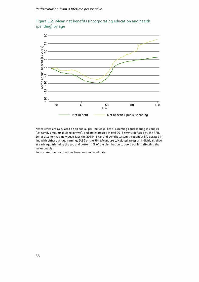
Redistribution from a lifetime perspective
88
Figure E.2. Mean net benefits (incorporating education and health
spending) by age
Note: Series are calculated on an annual per-individual basis, assuming equal sharing in couples
(i.e. family amounts divided by two), and are expressed in real 2015 terms (deflated by the RPI).
Series assume that individuals face the 2015/16 tax and benefit system throughout life uprated in
line with either average earnings (AEI) or the RPI. Means are calculated across all individuals alive
at each age, trimming the top and bottom 1% of the distribution to avoid outliers affecting the
series unduly.
Source: Authors’ calculations based on simulated data.
-20
-15
-10
-50
51
01
52
0M
ea
n a
nn
ua
l b
en
efi
t (£
k 2
01
5)
20 40 60 80 100Age
Net benefit Net benefit + public spending

89
© Institute for Fiscal Studies
F. Comparing the synthetic cross-section
with the LCFS
In this appendix, we compare our simulated 2015/16 cross-section (constructed using our simulated lifecycles) to data from actual LCFS cross-sections in 1978 and 2012. We uprate all relevant variables from the LCFS cross-sections to 2015 terms using average earnings. Table F.1 compares various characteristics across the different data sets. Individuals in our simulated cross-section tend to be slightly older on average than individuals in 1978 and 2012 (owing to the fact that our cohort of interest is predicted to be longer lived than previous cohorts). Other cohort differences mean that averages for our simulated cross-section fall between the averages for 1978 and 2012. For example, individuals in the baby-boom cohort tend to be more educated than the population in 1978 but less educated than those in 2012. They are also more likely to be renters than those in 2012, but less likely than those in 1978. In terms of family composition, our simulated cross-section is more similar to the 1978 population than the 2012 population with fewer lone parents than either. The lower number of children relative to the 1978 population is due to the fact that our simulated cross-section has a larger elderly population. Table F.1. Comparison of simulated cross-section with 1978 and 2012
LCFS
Note: Incomes uprated to 2015 terms in line with average earnings (AEI). Net and gross incomes
are equivalised for family size using the modified OECD equivalence scale. Gross income comprises
earnings and private pensions.
Source: Authors’ calculations based on simulated data and the LCFS (and previous surveys).
Simulated LCFS 1978 LCFS 2012
Age 51 46 48
Childless single 32% 29% 40%
Childless couple 42% 37% 32%
Lone parent 1% 2% 8%
Couple parent 25% 32% 20%
Number of children 0.47 0.64 0.47
Employed 55% 63% 58%
Average weekly earnings £540.99 £571.41 £545.75
Renter 28% 44% 25%
Education: GCSEs 62% 83% 52%
Education: A-levels 28% 9% 18%
Education: university 10% 7% 30%
Gini: eq. net income 0.305 0.302 0.301
Gini: eq. gross income 0.523 0.484 0.565

Redistribution from a lifetime perspective
90
In terms of inequality of net incomes, our three data sets are essentially identical. Inequality of gross incomes (defined for comparability across the different data sets as earnings plus private pensions – the two income sources we consider in our pooled cross-section) again lies between the 1978 and 2012 LCFS. The numbers for the simulated cross-section differ from those reported in Table 3.1 as they are calculated across households rather than individuals to make them comparable to the values from the LCFS. Figure F.1 shows the distribution of gross incomes (above zero) across the three populations. Once incomes for the 1978 and 2012 LCFS have been uprated to 2015 terms, incomes tend to be higher for those at the bottom in the 1978 data and higher for those at the top in the 2012 data. Incomes in our simulated cross-section tend to be slightly lower in the middle of the income distribution than in the other two populations. Figure F.1. Income distributions for simulated cross-section and LCFS in
1978 and 2012
Note: Incomes include earnings and private pensions, are equivalised for family size using the
modified OECD equivalence scale and uprated to 2015 terms in line with average earnings (AEI).
Source: Authors’ calculations based on simulated data and the LCFS (and previous surveys).
02
04
06
08
01
00
Pe
rce
nti
le
0 500 1000 1500 2000Weekly gross income
Simulated LCFS 1978
LCFS 2012