reduced-hessian methods for constrained optimization · reduced-hessian methods signi cance of p k...
TRANSCRIPT

Reduced-Hessian Methods for ConstrainedOptimization
Philip E. Gill
University of California, San Diego
Joint work with:Michael Ferry & Elizabeth Wong
11th US & Mexico Workshop on Optimization and its ApplicationsHuatulco, Mexico, January 8–12, 2018.
UC San Diego | Center for Computational Mathematics 1/45

Our honoree . . .
UC San Diego | Center for Computational Mathematics 2/45

Outline
1 Reduced-Hessian Methods for Unconstrained Optimization
2 Bound-Constrained Optimization
3 Quasi-Wolfe Line Search
4 Reduced-Hessian Methods for Bound-Constrained Optimization
5 Some Numerical Results
UC San Diego | Center for Computational Mathematics 3/45

Reduced-Hessian Methodsfor Unconstrained Optimization
UC San Diego | Center for Computational Mathematics 4/45
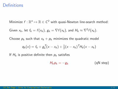
Definitions
Minimize f : Rn 7→ R ∈ C 2 with quasi-Newton line-search method:
Given xk , let fk = f (xk), gk = ∇f (xk), and Hk ≈ ∇2f (xk).
Choose pk such that xk + pk minimizes the quadratic model
qk(x) = fk + gTk (x − xk) + 1
2(x − xk)THk(x − xk)
If Hk is positive definite then pk satisfies
Hkpk = −gk (qN step)
UC San Diego | Center for Computational Mathematics 5/45

Definitions
Define xk+1 = xk + αkpk where αk is obtained from line search on
φk(α) = f (xk + αpk)
• Armijo condition:
φk(α) < φk(0) + ηAαφ′k(0), ηA ∈ (0, 12)
• (strong) Wolfe conditions:
φk(α) < φk(0) + ηAαφ′k(0), ηA ∈ (0, 12)
|φ′k(α)| ≤ ηW |φ′k(0)|, ηW ∈ (ηA, 1)
UC San Diego | Center for Computational Mathematics 6/45
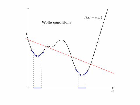
α
f(xk + αpk)
Wolfe conditions

Quasi-Newton Methods
Updating Hk :
• H0 = σIn where σ > 0
• Compute Hk+1 as the BFGS update to Hk , i.e.,
Hk+1 = Hk −1
sTk HkskHksks
Tk Hk +
1
yTk skyky
Tk ,
where sk = xk+1 − xk , yk = gk+1 − gk , and yTk skapproximates the curvature of f along pk .
• Wolfe condition guarantees that Hk can be updated.
One option to calculate pk :
• Store upper-triangular Cholesky factor Rk where RTk Rk = Hk
UC San Diego | Center for Computational Mathematics 8/45

Reduced-Hessian Methods
(Fenelon, 1981 and Siegel, 1992)
Let Gk = span(g0, g1, . . . , gk) and G⊥k be the orthogonalcomplement of Gk in Rn.
Result
Consider a quasi-Newton method with BFGS update applied to ageneral nonlinear function. If H0 = σI (σ > 0), then:
• pk ∈ Gk for all k .
• If z ∈ Gk and w ∈ G⊥k , then Hkz ∈ Gk and Hkw = σw .
UC San Diego | Center for Computational Mathematics 9/45

Reduced-Hessian Methods
Significance of pk ∈ Gk :
• No need to minimize the quadratic model over the full space.
• Search directions lie in an expanding sequence of subspaces.
Significance of Hkz ∈ Gk and Hkw = σw :
• Curvature stored in Hk along any unit vector in G⊥k is σ.
• All nontrivial curvature information in Hk can be stored in asmaller rk × rk matrix, where rk = dim(Gk).
UC San Diego | Center for Computational Mathematics 10/45
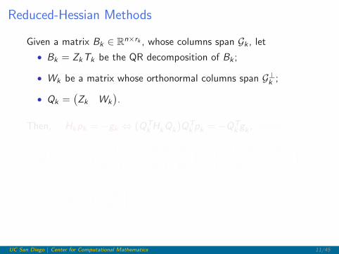
Reduced-Hessian Methods
Given a matrix Bk ∈ Rn×rk , whose columns span Gk , let
• Bk = ZkTk be the QR decomposition of Bk ;
• Wk be a matrix whose orthonormal columns span G⊥k ;
• Qk =(Zk Wk
).
Then, Hkpk = −gk ⇔ (QTkHkQk)QT
k pk = −QTk gk , where
QTkHkQk =
(ZTk HkZk ZT
k HkWk
W Tk HkZk W T
k HkWk
)=
(ZTk HkZk 0
0 σIn−rk
)
QTk gk =
(ZTk gk0
).
UC San Diego | Center for Computational Mathematics 11/45

Reduced-Hessian Methods
A reduced-Hessian (RH) method obtains pk from
pk = Zkqk where qk solves ZTk HZkqk = −ZT
k gk , (RH step)
which is equivalent to (qN step).
In practice, we use a Cholesky factorization RTk Rk = ZT
k HkZk .
• The new gradient gk+1 is accepted iff ‖(I − ZkZTk )gk+1‖ > ε.
• Store and update Zk , Rk , ZTk pk , ZT
k gk , and ZTk gk+1.
UC San Diego | Center for Computational Mathematics 12/45

Hk = QkQTk HkQkQ
Tk
=(Zk Wk
)(ZTk HkZk 0
0 σIn−rk
)(Zk
Wk
)
= Zk(ZTk HkZk)ZT
k + σ(I − ZkZTk ).
⇒ any z such that ZTk z = 0 satisfies Hkz = σz .
UC San Diego | Center for Computational Mathematics 13/45

Reduced-Hessian Method Variants
Reinitialization: If gk+1 6∈ Gk , the Cholesky factor Rk is updated as
Rk+1 ←(Rk 00√σk+1
),
where σk+1 is based on the latest estimate of the curvature, e.g.,
σk+1 =yTk sksTk sk
.
Lingering: restrict search direction to a smaller subspace and allowthe subspace to expand only when f is suitably minimized on thatsubspace.
UC San Diego | Center for Computational Mathematics 14/45
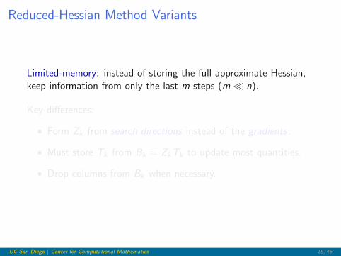
Reduced-Hessian Method Variants
Limited-memory: instead of storing the full approximate Hessian,keep information from only the last m steps (m� n).
Key differences:
• Form Zk from search directions instead of the gradients.
• Must store Tk from Bk = ZkTk to update most quantities.
• Drop columns from Bk when necessary.
UC San Diego | Center for Computational Mathematics 15/45

Main idea:
Maintain Bk = ZkTk , where Bk is the m × n matrix
Bk =(pk−m+1 pk−m+2 · · · pk−1 pk
)
with m� n (e.g., m = 5).
Bk = ZkTk is not available until pk has been computed.
However, if Zk is a basis for span(pk−m+1, . . . , pk−1, pk)
then it is also a basis for span(pk−m+1, . . . , pk−1, gk),
i.e., only the triangular factor associated with the (common) basisfor each of these subspaces will be different.
UC San Diego | Center for Computational Mathematics 16/45

At the start of iteration k, suppose we have the factors of
B(g)k =
(pk−m+1 pk−m+2 · · · pk−1 gk
)
• Compute pk .
• Swap pk with gk to give the factors of
Bk =(pk−m+1 pk−m+2 · · · pk−1 pk
)
• Compute xk+1, gk+1, etc., using a Wolfe line search.
• Update and reinitialize the factor Rk .
• If gk+1 is accepted, compute the factors of
B(g)k+1 =
(pk−m+2 pk−m+2 · · · pk gk+1
)
UC San Diego | Center for Computational Mathematics 17/45

Summary of key differences:
• Form Zk from search directions instead of gradients.
• Must store Tk from Bk = ZkTk to update most quantities.
• Can store Bk instead of Zk .
• Drop columns from Bk when necessary.
• Half the storage of conventional limited-memory approaches.
Retains finite termination property for quadratic f
(both with and without reinitialization).
UC San Diego | Center for Computational Mathematics 18/45

Bound-Constrained Optimization
UC San Diego | Center for Computational Mathematics 19/45
Bound Constraints
Given `, u ∈ Rn, solve
minimizex∈Rn
f (x) subject to ` ≤ x ≤ u.
Focus on line-search methods that use the BFGS method:
• Projected-gradient [Byrd, Lu, Nocedal, Zhu (1995)]
• Projected-search [Bertsekas (1982)]
These methods are designed to move on and off constraints rapidlyand identify the active set after a finite number of iterations.
UC San Diego | Center for Computational Mathematics 20/45

Projected-Gradient Methods
UC San Diego | Center for Computational Mathematics 21/45

Definitions
A(x) = {i : xi = `i or xi = ui}
Define the projection P(x) componentwise, where
[P(x)]i =
`i if xi < `i ,
ui if xi > ui ,
xi otherwise.
Given an iterate xk , define the piecewise linear paths
x−gk (α) = P(xk − αgk) and xpk (α) = P(xk + αpk)
UC San Diego | Center for Computational Mathematics 22/45

Algorithm L-BFGS-B
Given xk and qk(x), a typical iteration of L-BFGS-B looks like:
xk−gk
Move along projected path x−gk (α)
UC San Diego | Center for Computational Mathematics 23/45

Algorithm L-BFGS-B
Given xk and qk(x), a typical iteration of L-BFGS-B looks like:
xk−gk
xck
Find xck , the first point that minimizes qk(x) along x−gk (α)
UC San Diego | Center for Computational Mathematics 23/45
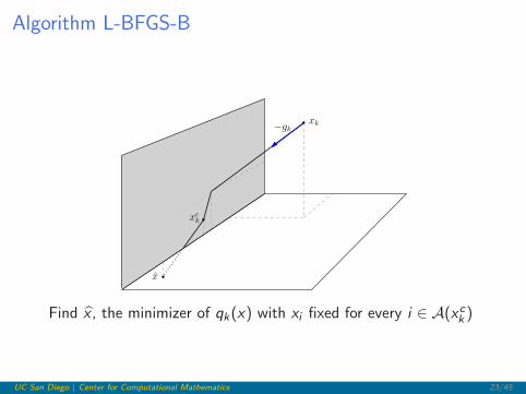
Algorithm L-BFGS-B
Given xk and qk(x), a typical iteration of L-BFGS-B looks like:
xk−gk
xck
x̂
Find x̂ , the minimizer of qk(x) with xi fixed for every i ∈ A(xck )
UC San Diego | Center for Computational Mathematics 23/45

Algorithm L-BFGS-B
Given xk and qk(x), a typical iteration of L-BFGS-B looks like:
xk−gk
xck
x̂
x̄
Find x̄ by projecting x̂ onto the feasible region
UC San Diego | Center for Computational Mathematics 23/45

Algorithm L-BFGS-B
Given xk and qk(x), a typical iteration of L-BFGS-B looks like:
xk−gk
xck
x̂
pk
x̄
Wolfe line search along pk with αmax = 1 to ensure feasibility
UC San Diego | Center for Computational Mathematics 23/45

Projected-Search Methods
UC San Diego | Center for Computational Mathematics 24/45

Definitions
A(x) = {i : xi = `i or xi = ui}
W(x) = {i : (xi = `i and gi > 0) or (xi = ui and gi < 0)}
Given a point x and vector p, the projected vector of p at x ,Px(p), is defined componentwise, where
[Px(p)]i =
{0 if i ∈ W(x),
pi otherwise.
Given a subspace S, the projected subspace of S at x is defined as
Px(S) = {Px(p) : p ∈ S}.
UC San Diego | Center for Computational Mathematics 25/45

Projected-Search Methods
A typical projected-search method updates xk as follows:
• Compute W(xk)
• Calculate pk as the solution of
minp∈Pxk
(Rn)qk(xk + p)
• Obtain xk+1 from an Armijo-like line search onψ(α) = f (xpk (α))
UC San Diego | Center for Computational Mathematics 26/45

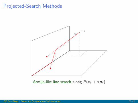
Projected-Search Methods
Given xk and f (x), a typical iteration looks like:
pkxk
UC San Diego | Center for Computational Mathematics 27/45

Projected-Search Methods
Given xk and f (x), a typical iteration looks like:
pkxk
UC San Diego | Center for Computational Mathematics 27/45
Projected-Search Methods
Given xk and f (x), a typical iteration looks like:
pkxk
Armijo-like line search along P(xk + αpk)
UC San Diego | Center for Computational Mathematics 27/45

Quasi-Wolfe Line Search
UC San Diego | Center for Computational Mathematics 28/45

Can’t use Wolfe conditions: ψ(α) is a continuous, piecewisedifferentiable function with cusps where xpk (α) changes direction.
As ψ(α) = f(xp(α)
)is only piecewise differentiable, it is not
possible to know when an interval contains a Wolfe step.
UC San Diego | Center for Computational Mathematics 29/45

Definition
Let ψ′−(α) and ψ′+(α) denote left- and right-derivatives of ψ(α).
Define a [strong] quasi-Wolfe step to be an Armijo-like step thatsatisfies at least one of the following conditions:
• |ψ′−(α)| ≤ ηW |ψ′+(0)|
• |ψ′+(α)| ≤ ηW |ψ′+(0)|
• ψ′−(α) ≤ 0 ≤ ψ′+(α)
UC San Diego | Center for Computational Mathematics 30/45

Theory
Analogous conditions for the existence of the Wolfe step imply theexistence of the quasi-Wolfe step.
Quasi-Wolfe line searches are ideal for projected-search methods.
If ψ is differentiable the quasi-Wolfe and Wolfe conditions areidentical.
In rare cases, Hk cannot be updated after quasi-Wolfe step.
UC San Diego | Center for Computational Mathematics 31/45
Reduced-Hessian Methods forBound-Constrained Optimization
UC San Diego | Center for Computational Mathematics 32/45
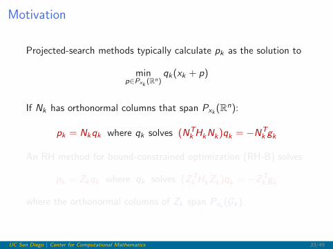
Motivation
Projected-search methods typically calculate pk as the solution to
minp∈Pxk
(Rn)qk(xk + p)
If Nk has orthonormal columns that span Pxk (Rn):
pk = Nkqk where qk solves (NTkHkNk)qk = −NT
k gk
An RH method for bound-constrained optimization (RH-B) solves
pk = Zkqk where qk solves (ZTk HkZk)qk = −ZT
k gk
where the orthonormal columns of Zk span Pxk (Gk).
UC San Diego | Center for Computational Mathematics 33/45
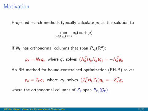

Details
Builds on limited-memory RH method framework, plus:
• Update values dependent on Bk when Wk 6=Wk−1
• Use projected-search trappings (working set, projections, ...).
• Use line search compatible with projected-search methods.
• Update Hk with curvature in direction restricted torange(Zk+1).
UC San Diego | Center for Computational Mathematics 34/45
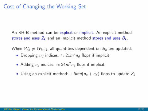
Cost of Changing the Working Set
An RH-B method can be explicit or implicit. An explicit methodstores and uses Zk and an implicit method stores and uses Bk .
When Wk 6=Wk−1, all quantities dependent on Bk are updated:
• Dropping nd indices: ≈ 21m2nd flops if implicit
• Adding na indices: ≈ 24m2na flops if implicit
• Using an explicit method: +6mn(na + nd) flops to update Zk
UC San Diego | Center for Computational Mathematics 35/45

Some Numerical Results
UC San Diego | Center for Computational Mathematics 36/45
Results
LRH-B (v1.0) and LBFGS-B (v3.0)
LRH-B implemented in Fortran 2003; LBFGS-B in Fortran 77.
373 problems from CUTEst test set, with n between 1 and 192, 627.
Termination: ‖Pxk (gk)‖∞ < 10−5 or 300K itns or 1000 cpu secs.
UC San Diego | Center for Computational Mathematics 37/45

Implementation
Algorithm LRH-B (v1.0):
• Limited-memory: restricted to m preceding search directions.
• Reinitialization: included if n > min(6,m).
• Lingering: excluded.
• Method type: implicit.
• Updates: Bk , Tk , Rk updated for all Wk 6=Wk−1.
UC San Diego | Center for Computational Mathematics 38/45

Default parameters
0 2 4 6 8 100
0.1
0.2
0.3
0.4
0.5
0.6
0.7
0.8
0.9
1
Function evaluations for 374 UC/BC problems
LBFGS-B m = 5
LRH-B m = 10
0 2 4 6 8 10
Times for 374 UC/BC problems
LBFGS-B m = 5
LRH-B m = 10
1
0.9
0.8
0.7
0.6
0.5
0.4
0.3
0.2
0.1
Name m Failed
LBFGS-B 5 78
LRH-B 10 49
UC San Diego | Center for Computational Mathematics 39/45

0 2 4 6 8 10
0.1
0.2
0.3
0.4
0.5
0.6
0.7
0.8
0.9
1
Function evaluations for 374 UC/BC problems
LBFGS-B m = 5
LRH-B m = 5
0 2 4 6 8 10
Times for 374 UC/BC problems
LBFGS-B m = 5
LRH-B m = 5
1
0.9
0.8
0.7
0.6
0.5
0.4
0.3
0.2
0.1
Name m Failed
LBFGS-B 5 78
LRH-B 5 50
UC San Diego | Center for Computational Mathematics 40/45

0 1 2 3 4 5 6 7 8 90
0.1
0.2
0.3
0.4
0.5
0.6
0.7
0.8
0.9
1
Function evaluations for 374 UC/BC problems
LBFGS-B m = 10
LRH-B m = 10
0 2 4 6 8 10
Times for 374 UC/BC problems
LBFGS-B m = 10
LRH-B m = 10
1
0.9
0.8
0.7
0.6
0.5
0.4
0.3
0.2
0.1
Name m Failed
LBFGS-B 10 78
LRH-B 10 49
UC San Diego | Center for Computational Mathematics 41/45

0 2 4 6 8 10
0.1
0.2
0.3
0.4
0.5
0.6
0.7
0.8
0.9
1
Function evaluations for 374 UC/BC problems
LBFGS-B m = 5
LBFGS-B m = 10
LRH-B m = 5
LRH-B m = 10
0 2 4 6 8 10
0.1
0.2
0.3
0.4
0.5
0.6
0.7
0.8
0.9
1
LBFGS-B m = 5
LBFGS-B m = 10
LRH-B m = 5
LRH-B m = 10
Times for 374 UC/BC problems
UC San Diego | Center for Computational Mathematics 42/45

Outstanding Issues
• Projected-search methods:
• When to update/factor?
Better to refactor when there are lots of changes to A.
• Implement plane rotations via level-two BLAS.
• How complex should we make the quasi-Wolfe search?
UC San Diego | Center for Computational Mathematics 43/45

Thank you!
UC San Diego | Center for Computational Mathematics 44/45

ReferencesD. P. Bertsekas, Projected Newton methods for optimization problems with simpleconstraints, SIAM J. Control Optim., 20:221–246, 1982.
R. Byrd, P. Lu, J. Nocedal and C. Zhu, A limited-memory algorithm for boundconstrained optimization, SIAM J. Sci. Comput. 16:1190–1208, 1995.
M. C. Fenelon, Preconditioned conjugate-gradient-type methods for large-scaleunconstrained optimization, Ph.D. thesis, Department of Operations Research,Stanford University, Stanford, CA, 1981.
M. W. Ferry, P. E. Gill and E. Wong, A limited-memory reduced Hessian method forbound-constrained optimization, Report CCoM 18-01, Center for ComputationalMathematics, University of California, San Diego, 2018 (to appear).
P. E. Gill and M. W. Leonard, Reduced-Hessian quasi-Newton methods forunconstrained optimization, SIAM J. Optim., 12:209–237, 2001.
P. E. Gill and M. W. Leonard, Limited-memory reduced-Hessian methods forunconstrained optimization, SIAM J. Optim., 14:380–401, 2003.
J. Morales and J. Nocedal, Remark on “Algorithm 778: L-BFGS-B: Fortransubroutines for large-scale bound constrained optimization”, ACMTrans. Math. Softw., 38(1)7:1–7:4, 2011.
D. Siegel, Modifying the BFGS update by a new column scaling technique,Math. Program., 66:45–78, 1994.
UC San Diego | Center for Computational Mathematics 45/45