reduced mandated inspection by remote field eddy current ... library/research/oil-gas/natural...
TRANSCRIPT

DE-FC26-04NT42266 Final Report - GTI
Reduced Mandated Inspection by Remote Field Eddy Current Inspection of Unpiggable Pipelines
T e c h n i c a l F i n a l R e p o r t
Reporting Period Start Date: October 1, 2005 Reporting Period End Date: September 30, 2006
GTI Project Manager: Albert Teitsma GTI Principal Investigator: Julie Maupin
October 2006
DE-FC26-04NT42266
Prepared by:
Gas Technology Institute 1700 S. Mount Prospect Road
Des Plaines, Illinois 60018

DE-FC26-04NT42266 Final Report - GTI
DISCLAIMER This report was prepared as an account of work sponsored by an agency of the
United States Government. Neither the United States Government nor any
agency thereof, nor any of their employees, make any warranty, express or
implied, or assumes any legal liability or responsibility for the accuracy,
completeness, or usefulness of any information, apparatus, product, or process
disclosed, or represents that its use would not infringe privately owned rights.
Reference herein to any specific commercial product, process, or service by
trade name, trademark, manufacturer, or otherwise does not necessarily
constitute or imply its endorsement, recommendation, or favoring by the United
States Government or any agency thereof. The views and opinions of authors
expressed herein do not necessarily state or reflect those of the United States
Government or any agency thereof.

Page 3
TABLE OF CONTENTS DISCLAIMER ....................................................................................................2 TABLE OF CONTENTS ....................................................................................3 EXECUTIVE SUMMARY...................................................................................4 THE REMOTE FIELD EDDY CURRENT TECHNIQUE ....................................5 PROJECT OBJECTIVES ..................................................................................8 NON EXPERIMENTAL......................................................................................9 EXPERIMENTAL.............................................................................................10
ELECTRONICS and DATA ACQUISITION IMPROVEMENTS....................11 LAB APPARATUS .......................................................................................11 GEOMETRIC & SYSTEM STUDIES ...........................................................12 DRIVE COIL DESIGN OPTIMIZATION .......................................................12 FINITE ELEMENT ANALYSIS CALCULATIONS.........................................15
RESULTS AND DISCUSSION........................................................................18 WORK PERFORMED ON 6” PIPE ..............................................................18 DIFFERENTIAL COIL TESTING .................................................................20 EXCITER COIL 5 TESTING ........................................................................23 EXCITER COIL 6 TESTING ........................................................................24 EXCITER COIL 7 TESTING ........................................................................26 ASSESSMENT OF EXCITER COILS ..........................................................30 RUSSELL FERROSCOPE ..........................................................................31 MECHANICAL DESIGN ..............................................................................44 PROTOTYPE...............................................................................................54 ELECTRONIC DESIGN AND IMPLIMENTATION.......................................58
CONCLUSION ................................................................................................62 REFERENCES................................................................................................63 TABLE OF FIGURES ......................................................................................64
Page 4
EXECUTIVE SUMMARY
The Remote Field Eddy Current (RFEC) technique is ideal for inspecting unpiggable pipelines because all of its components can be made much smaller than the diameter of the pipe to be inspected. For this reason, RFEC was chosen as a technology for unpiggable pipeline inspections by DOE-NETL with the support of OTD and PRCI, to be integrated with platforms selected by DOE-NETL. As part of the project, the RFEC laboratory facilities were upgraded and data collection was made nearly autonomous. The resulting improved data collection speeds allowed GTI to test more variables to improve the performance of the combined RFEC and platform technologies. Tests were conducted on 6”, 8”, and 12” seamless and seam-welded pipes. Testing on the 6” pipes included using seven exciter coils, each of different geometry with an initial focus on preparing the technology for use on an autonomous robotic platform with limited battery capacity. Reductions in power consumption proved successful. Tests with metal components similar to the Explorer II modules were performed to check for interference with the electromagnetic fields. The results of these tests indicated RFEC would be able to produce quality inspections while on the robot. Mechanical constraints imposed by the platform, power requirements, control and communication protocols, and potential busses and connectors were addressed. Much work went into sensor module design including the mechanics and electronic diagrams and schematics. GTI participated in two Technology Demonstrations for inspection technologies held at Battelle Laboratories. GTI showed excellent detection and sizing abilities for natural corrosion. Following the demonstration, module building commenced but was stopped when funding reductions did not permit continued development for the selected robotic platform. Conference calls were held between GTI and its sponsors to resolve the issue of how to proceed with reduced funding. The project was rescoped for 10-16” pipes with the intent of looking at lower cost, easier to implement, tethered platform applications. OTD ended its sponsorship.
Page 5
THE REMOTE FIELD EDDY CURRENT TECHNIQUE The remote field eddy current (RFEC) technique was patented by W. R.
McLean (US Patent 2,573,799, “Apparatus for Magnetically Measuring Thickness
of Ferrous Pipe”, Nov.6, 1951) and first developed by Tom Schmidt at Shell for
down hole inspection (Schmidt, T. R., “The Casing Instrument Tool- …”,
Corrosion, pp 81-85, July 1961). The RFEC technology has many advantages
including:
A simple exciter coil that can be less than one-third of the pipe diameter. The exciter coil does not need to be close to the wall. [3 pt spacing]
Simple and small (millimeter to centimeter diameter) sensor coils that do not need to contact the wall. Thus, the diameter of the coil array can be easily adjusted to match the pipe diameter yet pass through a small opening.
Sensor coils close to the pipe wall provide sensitivity and accuracy comparable to standard MFL inspection tools. General pipe corrosion of 10% of the wall thickness or less is detected and measured with commercial units.
Sensor lift-off, up to 0.75 inch can be automatically compensated for, though sensitivity and resolution will be compromised.
The technique is commercially viable for inspecting boiler tubes and pipe
diameters up to 8 inches for several hundred feet. Russell Technologies
developed an 18 inch device that can inspect production wells for several
thousand feet. However, none of the current versions are collapsible to one-third
of the pipe diameter or less, nor can any handle short-radius elbows and other
obstacles. To adapt the technique for this application will require investigating
variations such as transmitter coil angle and methods for either reducing the
variations or sensitivity to them. Larger diameters should not be a problem since
specialized tools can inspect the steel reinforcing of 12 foot diameter concrete
water mains (Atherton, D. L., US patent 6,127,823, “Electromagnetic Method for
Non-Destructive Testing of Prestressed Concrete Pipes for Broken Prestressed
Wires”, Oct. 3, 2000).
Page 6
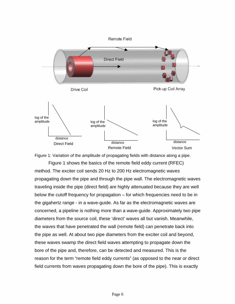
Figure 1: Variation of the amplitude of propagating fields with distance along a pipe.
Figure 1 shows the basics of the remote field eddy current (RFEC)
method. The exciter coil sends 20 Hz to 200 Hz electromagnetic waves
propagating down the pipe and through the pipe wall. The electromagnetic waves
traveling inside the pipe (direct field) are highly attenuated because they are well
below the cutoff frequency for propagation – for which frequencies need to be in
the gigahertz range - in a wave-guide. As far as the electromagnetic waves are
concerned, a pipeline is nothing more than a wave-guide. Approximately two pipe
diameters from the source coil, these ‘direct’ waves all but vanish. Meanwhile,
the waves that have penetrated the wall (remote field) can penetrate back into
the pipe as well. At about two pipe diameters from the exciter coil and beyond,
these waves swamp the direct field waves attempting to propagate down the
bore of the pipe and, therefore, can be detected and measured. This is the
reason for the term “remote field eddy currents” (as opposed to the near or direct
field currents from waves propagating down the bore of the pipe). This is exactly
distance
log of the amplitude
Direct Field distance
log of the amplitude
Remote Field distance
log of the amplitude
Vector Sum

Page 7
what is needed. Any pipeline flaws such as metal loss from corrosion or other
causes that affect the propagation of these RFECs back into the pipe alter the
detected signal so that the flaws may be detected and measured by the sensing
coils.
Figure 2: A simulated drawing of the RFEC technology integrated with Explorer. The RFEC frequencies need to be low since higher frequencies will not
penetrate ferromagnetic conductors such as pipeline steel. Methods to increase
penetration by lowering the magnetic permeability by magnetizing the pipe may
not work well for unpiggable pipelines for the some of the same reasons that
MFL inspection will not work well. The one disadvantage of the technique will
therefore be slow inspection speeds. Other than that, the RFEC technique is the
ideal in-line inspection technology for inspecting “unpiggable” pipelines. The
transmitter and sensors can be designed to fit through anything that robots or
any design of pig driving cups can pass through. Figure 2 shows a conceptual
design for a proposed inspection device using Explorer II to propel the tool

Page 8
through a distribution main. The exciter coil can be much smaller than the
pipeline diameter and mounted on a short module. Power and electronic
modules, including possibly a recharging module, can be mounted ahead and
between the transmitter and the sensors with additional modules, if needed,
following behind these. Modules at each end of the RFEC in-line inspection tool
can move the tool in either direction.
PROJECT OBJECTIVES The primary objective of this project was to develop Remote Field Eddy Current
methods for inspecting unpiggable pipelines. The first two research tasks were
writing a Research Management Plan and a Technology Status Assessment
Report. Task 3 called for proof of the feasibility of RFEC as an unpiggable
pipeline inspection technology. Additional objectives included Product Definition,
Electronics and Operational Prototype Development.

Page 9
NON EXPERIMENTAL
GTI completed Task 1, the Research Management Plan, which detailed
the work to be performed under this project. GTI also completed the technology
Assessment Report that described both the status of the RFEC technology and
where it fit within available technologies for enhancing pipeline reliability. The
feasibility of inspecting transmission pipelines using the RFEC technique was
proven early in the project. We proved the technique’s ability to use small
components, thereby confirming it suitable for unpiggable pipeline inspection.
The scope of work under this project included collaborative work with the
DOE-NETL selected platform designers. For much of the project, the Explorer II
robot at Carnegie Mellon University (CMU) was the target. This work consisted of
sensor/platform definition, where we drafted requirements of our sensor, created
three module designs using 3D modeling software for the mid phase design
review, and completed one design for the final design review. The final design
included electronic schematics and specifications as well as a complete bill of
materials. The final design review was held at CMU in December, 2005, at which
time, we had also completed our set of Sensor Module Commands for facilitation
of information exchange over the Explorer II CANbus.
When GTI received notice that its sensors would not be integrated with
Explorer II due to funding cuts at DOE, the project was rescoped slightly to
address 10-16” diameter pipes. The design team updated the rotating type
design for the larger scale. It increased the number of sensors and improved the
rotation mechanism and sensor arms. This latest design was built and is
discussed later in this report.
Additionally, GTI provided monthly reports and annual project update
presentations.
Page 10
EXPERIMENTAL
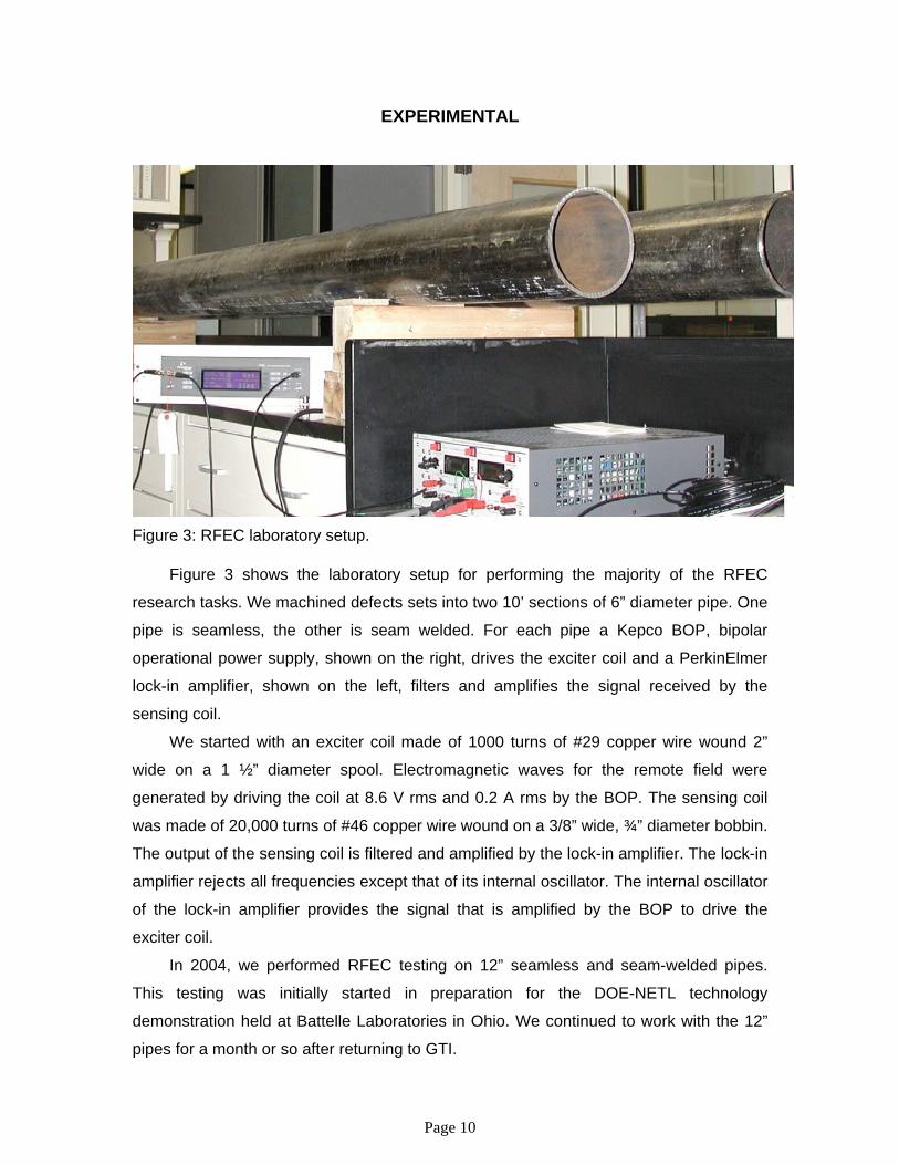
Figure 3: RFEC laboratory setup. Figure 3 shows the laboratory setup for performing the majority of the RFEC
research tasks. We machined defects sets into two 10’ sections of 6” diameter pipe. One
pipe is seamless, the other is seam welded. For each pipe a Kepco BOP, bipolar
operational power supply, shown on the right, drives the exciter coil and a PerkinElmer
lock-in amplifier, shown on the left, filters and amplifies the signal received by the
sensing coil.
We started with an exciter coil made of 1000 turns of #29 copper wire wound 2”
wide on a 1 ½” diameter spool. Electromagnetic waves for the remote field were
generated by driving the coil at 8.6 V rms and 0.2 A rms by the BOP. The sensing coil
was made of 20,000 turns of #46 copper wire wound on a 3/8” wide, ¾” diameter bobbin.
The output of the sensing coil is filtered and amplified by the lock-in amplifier. The lock-in
amplifier rejects all frequencies except that of its internal oscillator. The internal oscillator
of the lock-in amplifier provides the signal that is amplified by the BOP to drive the
exciter coil.
In 2004, we performed RFEC testing on 12” seamless and seam-welded pipes.
This testing was initially started in preparation for the DOE-NETL technology
demonstration held at Battelle Laboratories in Ohio. We continued to work with the 12”
pipes for a month or so after returning to GTI.
Page 11
Late in 2005, we rebuilt our laboratory vehicle to accommodate the sensors through
an 8” diameter pipe in preparation for a second demonstration at Battelle in January
2006. We achieved good results using the same exciter and sensing coils as we had
been using in the 6” pipe, further illustrating the ability to use RFEC coils that are much
smaller than the pipe diameter.
ELECTRONICS and DATA ACQUISITION IMPROVEMENTS We built a 16 channel multiplexer for use on the 6” pipes in the laboratory.
In order to collect data for 16 sensor coils, we updated our LabVIEW data
acquisition program to step through and record data from all 16 channels. The
LabVIEW program also controlled the location of the sensors and recorded
position data from the odometer at data acquisition locations.
Using the multiplexer board and LabVIEW significantly improved collection
speeds. Manually, it would take close to two hours to inspect a single defect.
Using the new autonomous system, all 13 defects along a 10’ section of pipe
could be inspected in an hour and a half without a researcher present. Further
improvements in inspection speeds were seen when GTI purchased and
employed a Ferroscope electronics circuit and software from Russell
Technologies, Inc. This is a much more sophisticated system as Russell has
years of experience using the RFEC technique to inspect boiler tubes. The
collection speeds for this setup are about 3 minutes for a 10’ length of pipe.
LAB APPARATUS We made improvements in the 6” vehicle. The original vehicle had one coil
mounted on an arm. To be able to mount multiple coils, we drilled equally spaced
holes into a 6” disc and mounted three sets of 5 coils each at 120° locations. This
new vehicle allowed us to scan all the defect sets at the same time using the
BOP and lock-in setup. We also installed a motor-encoder mechanism to
automate the data collection. In addition, a self-righting mechanism was put in
place to prevent major rotations of the vehicle. This eliminates the need to
“uncurl” the data during analysis.

Page 12
We attached a 4’ section of 6” PVC pipe to the starting end of the
seamless pipe. The PVC pipe has large windows cut out of it to facilitate
changing components on the vehicle. It also allows us to start taking
measurements from the zero mark rather than starting at 33". This lets us inspect
the defects located at 24” and 30” without pulling the RFEC vehicle through from
the other end.
In addition to the 6” vehicle, we built vehicles for 8” and 12” inspections.
GTI also built an apparatus to transport the Russell Equipment through 6” and 8”
pipe. The Russell equipment was demonstrated at the benchmarking test in
2006.
GEOMETRIC & SYSTEM STUDIES We studied drive and sensor coils separation distance as a function of
frequency. We obtained understandable results at frequencies up to about 2
KHz. We also studied defect detection at a set frequency as a function of sensor
orientation to pipe axis. The results of these studies are discussed in the results
section of this report. We wound and tested multiple exciter coils in both the 12”
and 6” pipes. These studies enabled us to reduce power consumption, which is
important for a tetherless robot, which has limited power.
DRIVE COIL DESIGN OPTIMIZATION
The 10”–16” RFEC design is for a tethered system, which does not have
the power restrictions of a robotic system. In that case, there is not the need to
balance power consumption versus defect detectability and the coil design can
be optimized as a function of frequency to maximize the magnetic dipole
moment. The frequency itself is selected primarily based on the magnetic
permeability and wall thickness of the pipe, but it can be adjusted for inspection
speed – higher frequency for higher speed – and/or transition zone location – the
location increases in distance from the drive coil with increasing frequency. A
conservative limit of about half an ampere per volt was set for the drive coil i.e. if

Page 13
the power supply for it put out 10 V, then the maximum current in the drive coil
would be about 5A.
The function of the drive coil is to generate a dipole moment given by
M=μrμ0NAi (1)
where M is the magnetic moment, μ0 is the permeability of free space, μr is the
relative magnetic permeability, N is the number of turns of wire on the coil, A is
the area of the coil, and i is alternating current.
i=v/Z (2)
where v is the alternating voltage, and Z is the complex impedance.
Z=R+jωL (3)
where R is the resistance, j is the square root of –1, and L is the inductance. For
a coil the resistance is given by the resistance per unit length times the wire
length. The resistance per unit length is obtained from the resistivity and the wire
diameter, which is determined by the wire gauge.
For a practical coil, the inductance is approximated by
L=μr dlr
Nr1096
8.0 22
++ (4)
Where ur is the relative magnetic permeability, r is the mean radius of the
coil, l is the length of the coil and d is the coil thickness, with the dimensions in
inches.
These equations along with those relating gauge to wire diameter, and
resistance per unit length to resistivity, were programmed into a Matlab program.
Matlab was used because it is matrix based and thus handles arrays of values
for the variables such as permeability, and wire diameters as simple variables.
The dipole moment was then calculated as a function of wire gauge, core
permeability and number of wire turns in the coil. The calculations were
compared to measured results.
Page 14
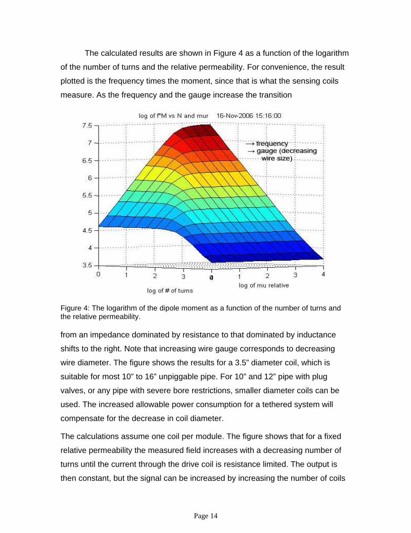
The calculated results are shown in Figure 4 as a function of the logarithm
of the number of turns and the relative permeability. For convenience, the result
plotted is the frequency times the moment, since that is what the sensing coils
measure. As the frequency and the gauge increase the transition
Figure 4: The logarithm of the dipole moment as a function of the number of turns and the relative permeability. from an impedance dominated by resistance to that dominated by inductance
shifts to the right. Note that increasing wire gauge corresponds to decreasing
wire diameter. The figure shows the results for a 3.5” diameter coil, which is
suitable for most 10” to 16” unpiggable pipe. For 10” and 12” pipe with plug
valves, or any pipe with severe bore restrictions, smaller diameter coils can be
used. The increased allowable power consumption for a tethered system will
compensate for the decrease in coil diameter.
The calculations assume one coil per module. The figure shows that for a fixed
relative permeability the measured field increases with a decreasing number of
turns until the current through the drive coil is resistance limited. The output is
then constant, but the signal can be increased by increasing the number of coils

Page 15
on the drive module until the current limit of the power supply is reached.
Increasing the permeability of the drive coil increases the signal until the current
is limited by the inductance.
Comparison to measured results agreed qualitatively with the calculations,
provided relative permeability values of around 10 are assumed.
FINITE ELEMENT ANALYSIS CALCULATIONS
Finite Element Analysis (FEA) can provide insight into how the
electromagnetic energy propagates through the bore or the pipe and how it
propagates outside the pipe wall and then returns to the inside of the pipe where
it can be detected by the sensing coils. It can quickly show how obstructions
affect the electromagnetic waves, and in detailed 3D calculation show the how
defects affect the electromagnetic radiation to generate the defect signals. One
important advantage of such calculations is the ability to see what is happening
to the electromagnetic fields in the pipe wall, a region not readily accessible
experimentally. GTI used the COMSOLAB multi-physics software package to
model a mockup of the RFEC inspection system developed for inspecting 6” to 8”
pipe.
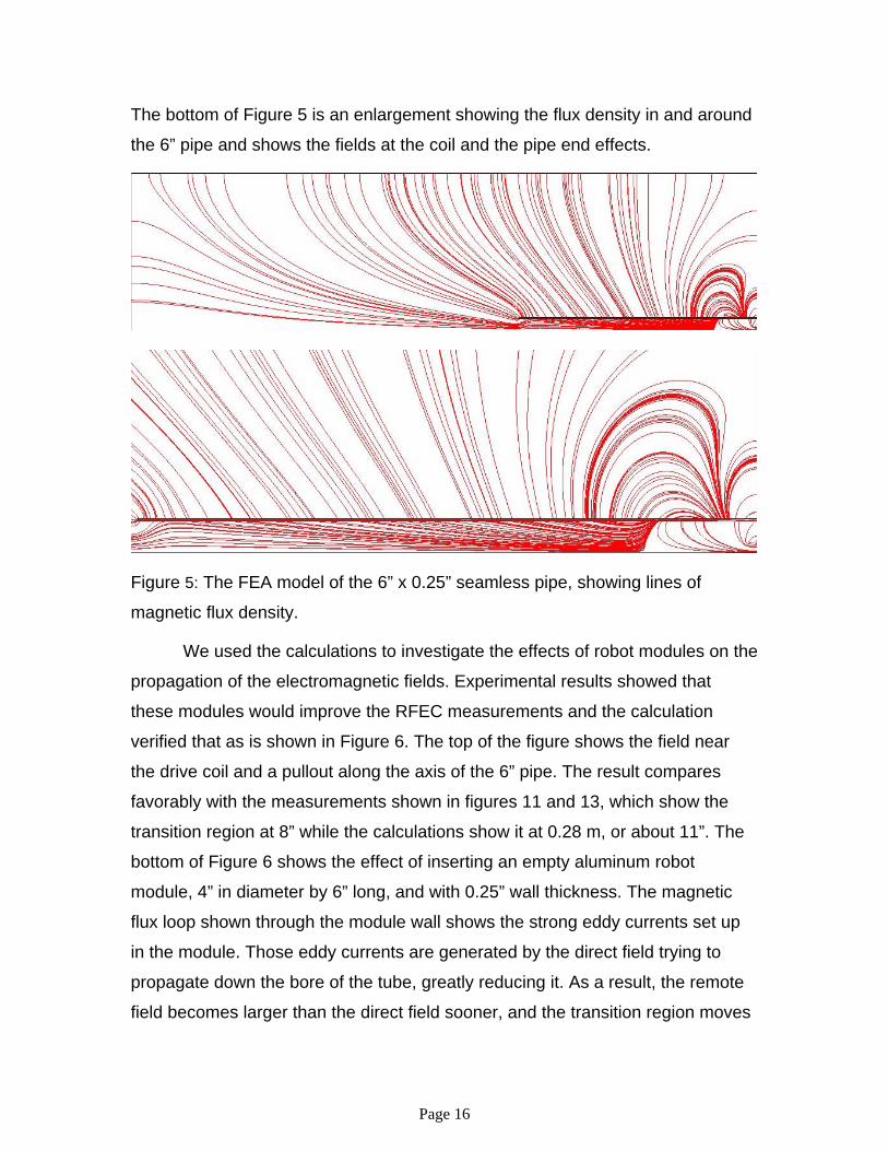
Figure 5 shows the magnetic flux density lines for a model of the 6”
diameter by 0.25” wall thickness 10’ long seamless steel pipe used in the NDE
laboratory for the RFEC experiments. Axial symmetry reduces the calculation to
a 2D calculation, while reflection symmetries reduce the calculation to a one
quarter model. The top view shows the full model. The electrical insulation
boundary conditions at the top and sides ensure that the magnetic flux meets the
boundaries at right angles there, as would be expected for flux lines far from the
source. There are places where it is obviously not quite correct, but these are far
enough from the regions of interest to not affect the calculations there. The drive
is a 2” diameter, 2” long coil at the right bottom corner (not visible), with 4000
ampere-turns of drive current. The frequency for the calculation was 50 Hz. The
pipe permeability was set at 100, which may be low, but the results seem
reasonable. The bottom of the model has the axial symmetry boundary condition.
Page 16
The bottom of Figure 5 is an enlargement showing the flux density in and around
the 6” pipe and shows the fields at the coil and the pipe end effects.
Figure 5: The FEA model of the 6” x 0.25” seamless pipe, showing lines of
magnetic flux density.
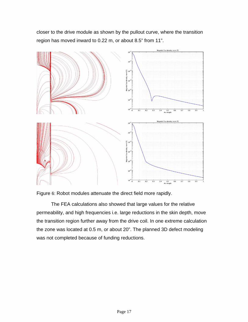
We used the calculations to investigate the effects of robot modules on the
propagation of the electromagnetic fields. Experimental results showed that
these modules would improve the RFEC measurements and the calculation
verified that as is shown in Figure 6. The top of the figure shows the field near
the drive coil and a pullout along the axis of the 6” pipe. The result compares
favorably with the measurements shown in figures 11 and 13, which show the
transition region at 8” while the calculations show it at 0.28 m, or about 11”. The
bottom of Figure 6 shows the effect of inserting an empty aluminum robot
module, 4” in diameter by 6” long, and with 0.25” wall thickness. The magnetic
flux loop shown through the module wall shows the strong eddy currents set up
in the module. Those eddy currents are generated by the direct field trying to
propagate down the bore of the tube, greatly reducing it. As a result, the remote
field becomes larger than the direct field sooner, and the transition region moves
Page 17
closer to the drive module as shown by the pullout curve, where the transition
region has moved inward to 0.22 m, or about 8.5” from 11”.
Figure 6: Robot modules attenuate the direct field more rapidly.
The FEA calculations also showed that large values for the relative
permeability, and high frequencies i.e. large reductions in the skin depth, move
the transition region further away from the drive coil. In one extreme calculation
the zone was located at 0.5 m, or about 20”. The planned 3D defect modeling
was not completed because of funding reductions.
Page 18
RESULTS AND DISCUSSION
WORK PERFORMED ON 6” PIPE
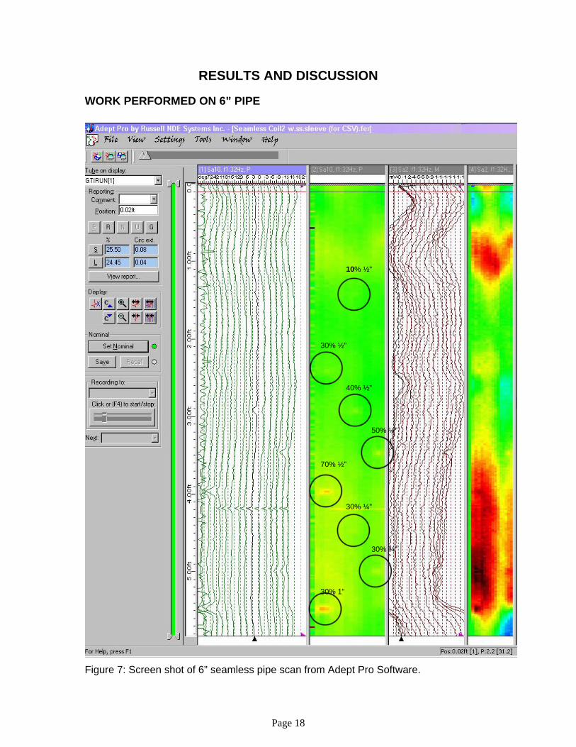
Figure 7: Screen shot of 6” seamless pipe scan from Adept Pro Software.
10% ½”
40% ½”
30% ½”
50% ½”
70% ½”
30% ¼”
30% ¾”
30% 1”
Page 19
Figure 7 is a scan of the entire 6” seamless pipe. During this test, a
stainless steel sleeve, was placed between the exciter and sensor coils. We were
testing the effect of metal components on detection results since robotic
components are metallic and size restrictions require at least one module
between the drive coil and the sensors. Our concern is that the metal could
disrupt the electromagnetic fields and produce poor results. In actuality, we
obtained better results with the sleeve inserted. This scan covered 10 defects.
Eight of them are identifiable in the strip chart to the left of the screenshot. The
two defects that did not show in the data were a 5% ½” and a 30% ¼” defect. We
suspect the 30% defect was not detected because we scan in ¼” steps. It is
likely that we stepped right over that defect. The results seem to be very
promising as the 10% ½” defect was found. We repeated this test with a chunk of
aluminum of 3” diameter and 3” in length between the exciter coil and sensing
coils. The results were slightly noisier but there was no apparent drop in the
amplitude of the signal. The smallest defect detected in this run was a 30% ½”
round.
Additional testing was performed on a rusting 6” lined Cast Iron pipe. The
RFEC technique has a broad range of applications in conducting and
ferromagnetic materials and we took advantage of an opportunity that came up to
demonstrate its capabilities. The technique was able to measure the remaining
wall thickness through the liner. Despite the Cast Iron appearing to have some
remaining wall thickness, the RFEC methods showed existing through wall
graphitization, which shows in Figure 8 as dark red.

Page 20
Figure 8: Screen shot of 6” lined Cast Iron.
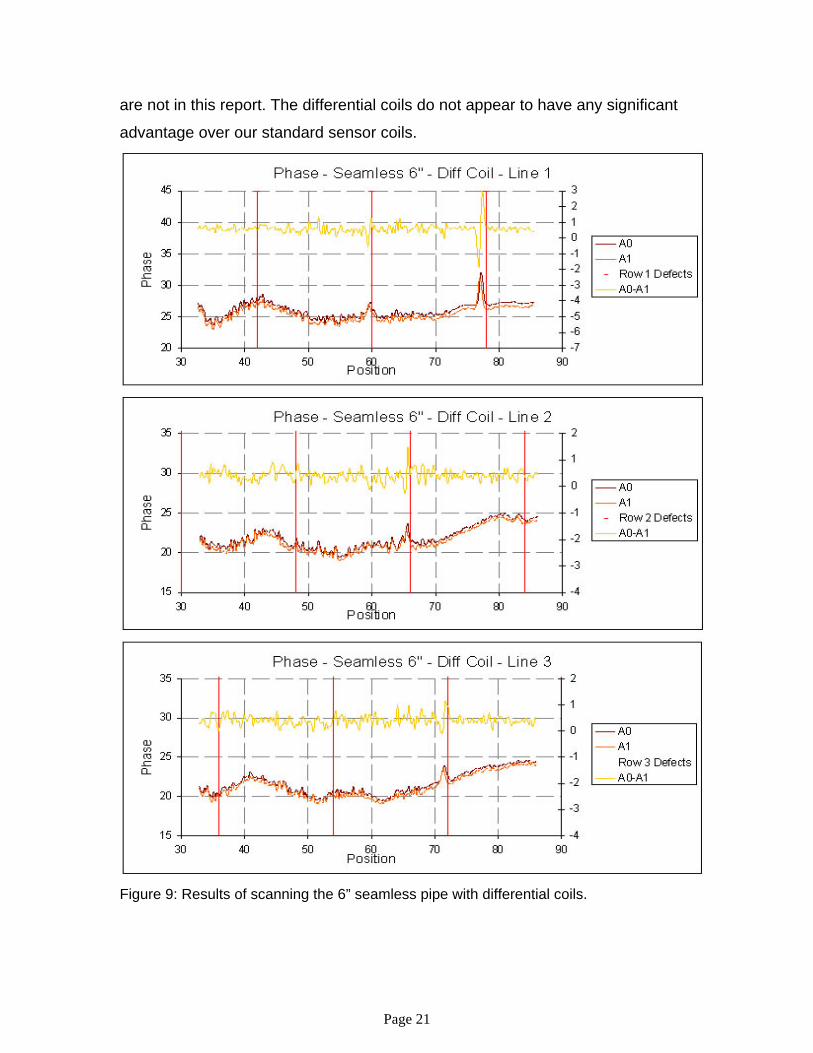
DIFFERENTIAL COIL TESTING
After completing the above testing with metal components, we performed
a study of differential coils. Our differential coils consisted of two identical coils
mounted close to each other on the same axis and were operated with each coil
180° out of phase with the other’s current. Data analysis included taking the
absolute measurement of each coil then subtracting them to get the differential.
Results of scanning the pipe along all three defect lines of the 6” seamless pipe
are shown in Figure 9. The absolute measurements are plotted in red and orange
and the differential measurement is plotted in yellow. The bright red vertical lines
represent defect locations along the length of the pipe. The defects measured
absolutely are indicated by significant increases in amplitude. A sharp drop
followed by a sharp increase in amplitude indicates differential defects. These
can be seen in Figure 9. The most obvious is the 80% deep defect located
around 78” on Line 1. Because of the length of the RFEC vehicle, we were
unable to scan the entire pipe in one pass. For each coil tested, we turned the
vehicle around and ran it through from the other end of the pipe. These results
Page 21
are not in this report. The differential coils do not appear to have any significant
advantage over our standard sensor coils.
Figure 9: Results of scanning the 6” seamless pipe with differential coils.
Page 22
Before beginning testing with exciter coil 5, we attached a 4’ section of 6”
PVC pipe to the starting end of the seamless pipe. It allowed us to take
measurements from the zero mark and we were able to inspect the defects
located at 24” and 30” without pulling the RFEC vehicle through from the other
end.
In addition to coil testing, we standardized our exciter coil - sensor coil
center-to-center distance to 15” based on the dimensions of the Explorer II
platform. Prior to this standardization, the center-to-center distance for each test
was based on pullout results of the individual exciter coils.
Page 23
EXCITER COIL 5 TESTING
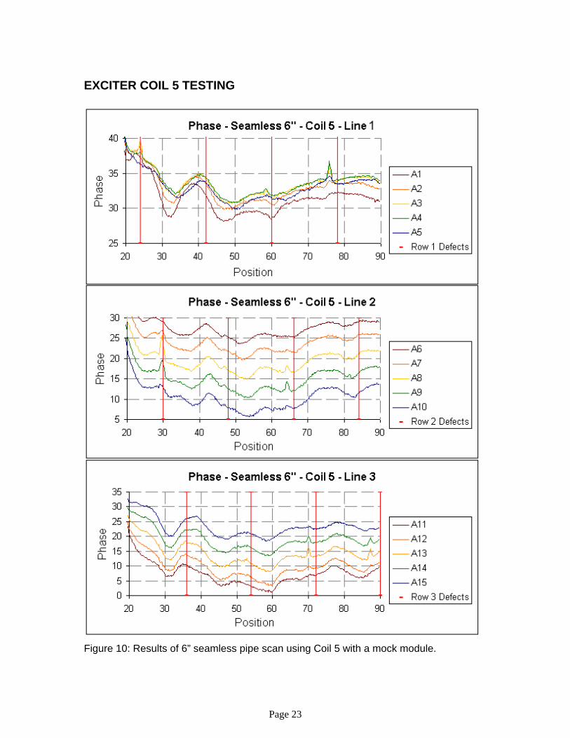
Figure 10: Results of 6” seamless pipe scan using Coil 5 with a mock module.
Page 24
Figure 10 shows the results of scanning the 6” pipe with Coil 5 as the
exciter coil. This test was performed with an imitation aluminum Explorer module
between the exciter coil and pick-up coils. This test was conducted to ensure that
the metal module would not cause an intolerable disruption of the RFEC signals.
We were pleased with the results in Figure 10. The defect locations are marked
with red vertical lines. An increase in the phase can be seen in at least one coil at
most defect locations. The defects that were not detected are the 5%, ½” at 42”
in line 1, the 30%, ¼” at 36” in line 3, and the 20%, ½” at 54” in line 3. None of
these defects would be repaired in the field.
EXCITER COIL 6 TESTING
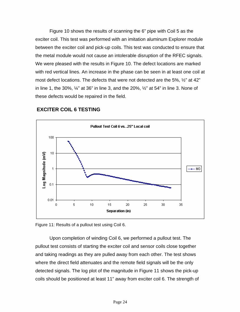
Figure 11: Results of a pullout test using Coil 6.
Upon completion of winding Coil 6, we performed a pullout test. The
pullout test consists of starting the exciter coil and sensor coils close together
and taking readings as they are pulled away from each other. The test shows
where the direct field attenuates and the remote field signals will be the only
detected signals. The log plot of the magnitude in Figure 11 shows the pick-up
coils should be positioned at least 11” away from exciter coil 6. The strength of
Page 25
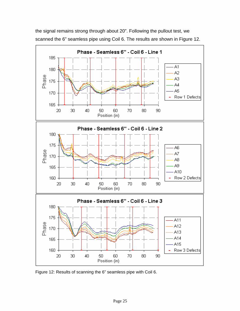
the signal remains strong through about 20”. Following the pullout test, we
scanned the 6” seamless pipe using Coil 6. The results are shown in Figure 12.
Figure 12: Results of scanning the 6” seamless pipe with Coil 6.
Page 26
The figure above shows scanning results of exciter coil 6 in the 6”
seamless pipe. The results are similar to Coil 5 results shown in Figure 10. Coil 6
detected all the defects Coil 5 and in addition, detected the 20%, ½” defect at 54”
in line 3. In other scans with Coil 6, we have seen detection of all defects with the
exception of the 5%, ½” defect.
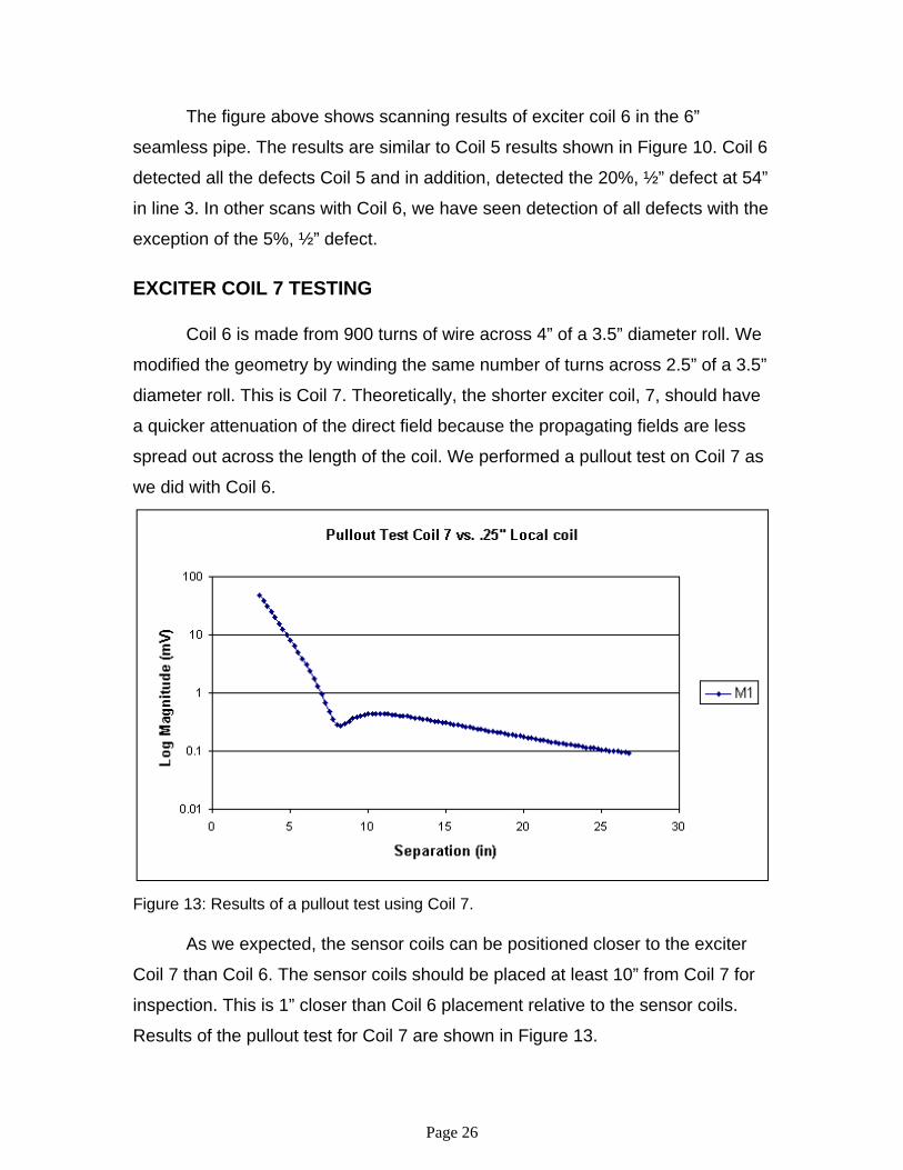
EXCITER COIL 7 TESTING Coil 6 is made from 900 turns of wire across 4” of a 3.5” diameter roll. We
modified the geometry by winding the same number of turns across 2.5” of a 3.5”
diameter roll. This is Coil 7. Theoretically, the shorter exciter coil, 7, should have
a quicker attenuation of the direct field because the propagating fields are less
spread out across the length of the coil. We performed a pullout test on Coil 7 as
we did with Coil 6.
Figure 13: Results of a pullout test using Coil 7. As we expected, the sensor coils can be positioned closer to the exciter
Coil 7 than Coil 6. The sensor coils should be placed at least 10” from Coil 7 for
inspection. This is 1” closer than Coil 6 placement relative to the sensor coils.
Results of the pullout test for Coil 7 are shown in Figure 13.

Page 27
Figure 14: Results of scanning the 6” seamless pipe with Coil 7.
Page 28
Figure 14 shows results obtained from scanning the 6” seamless pipe with
Coil 7 as the exciter coil. To date, Coil 7 has been the only exciter coil to detect
all 13 defects, including the 5% wt. Throughout the testing process, the data
obtained from scanning the seamless pipe tends to follow the same trends. At
the same time, there are also trends in the magnitude and phase data from the
welded pipe scans. The patterns in the welded pipe differ from the patterns seen
in the seamless pipe. We suspect the gradual rising and falling of the data is
attributed to permeability variation in each of the pipes, but could not eliminate
residual magnetic fields. In order to better understand the data and to have a set
of data to use as the base, we set up a baseline test. We laid both pipes parallel
to each other and ran subsequent tests using the same vehicle and lab
equipment. The first baseline test results are displayed in Figure 14. We
performed the first scan on the seamless pipe. Upon completion of that scan, we
transferred the RFEC vehicle to the welded pipe and performed a new scan on
the welded pipe. These results are shown in Figure 15 below.

Page 29
Figure 15: Results of scanning the 6” welded pipe with Coil 7.
Page 30
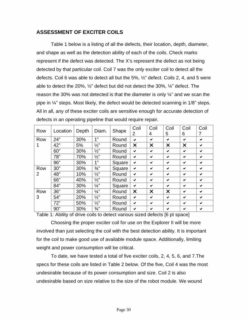
ASSESSMENT OF EXCITER COILS Table 1 below is a listing of all the defects, their location, depth, diameter,
and shape as well as the detection ability of each of the coils. Check marks
represent if the defect was detected. The X’s represent the defect as not being
detected by that particular coil. Coil 7 was the only exciter coil to detect all the
defects. Coil 6 was able to detect all but the 5%, ½” defect. Coils 2, 4, and 5 were
able to detect the 20%, ½” defect but did not detect the 30%, ¼” defect. The
reason the 30% was not detected is that the diameter is only ¼” and we scan the
pipe in ¼” steps. Most likely, the defect would be detected scanning in 1/8” steps.
All in all, any of these exciter coils are sensitive enough for accurate detection of
defects in an operating pipeline that would require repair.
Row Location Depth Diam. Shape Coil 2
Coil 4
Coil 5
Coil 6
Coil 7
24” 30% 1” Round a a a a a 42” 5% ½” Round r r r r a 60” 30% ½” Round a a a a a 78” 70% ½” Round a a a a a
Row 1
96” 30% 1” Square a a a a a 30” 30% ¾” Square a a a a a 48” 10% ½” Round a a a a a 66” 40% ½” Round a a a a a
Row 2
84” 30% ¼” Square a a a a a 36” 30% ¼” Round r r r a a 54” 20% ½” Round a a a a a 72” 50% ½” Round a a a a a
Row 3
90” 30% ¾” Round a a a a a Table 1: Ability of drive coils to detect various sized defects [6 pt space] Choosing the proper exciter coil for use on the Explorer II will be more
involved than just selecting the coil with the best detection ability. It is important
for the coil to make good use of available module space. Additionally, limiting
weight and power consumption will be critical.
To date, we have tested a total of five exciter coils, 2, 4, 5, 6, and 7.The
specs for these coils are listed in Table 2 below. Of the five, Coil 4 was the most
undesirable because of its power consumption and size. Coil 2 is also
undesirable based on size relative to the size of the robot module. We wound
Page 31
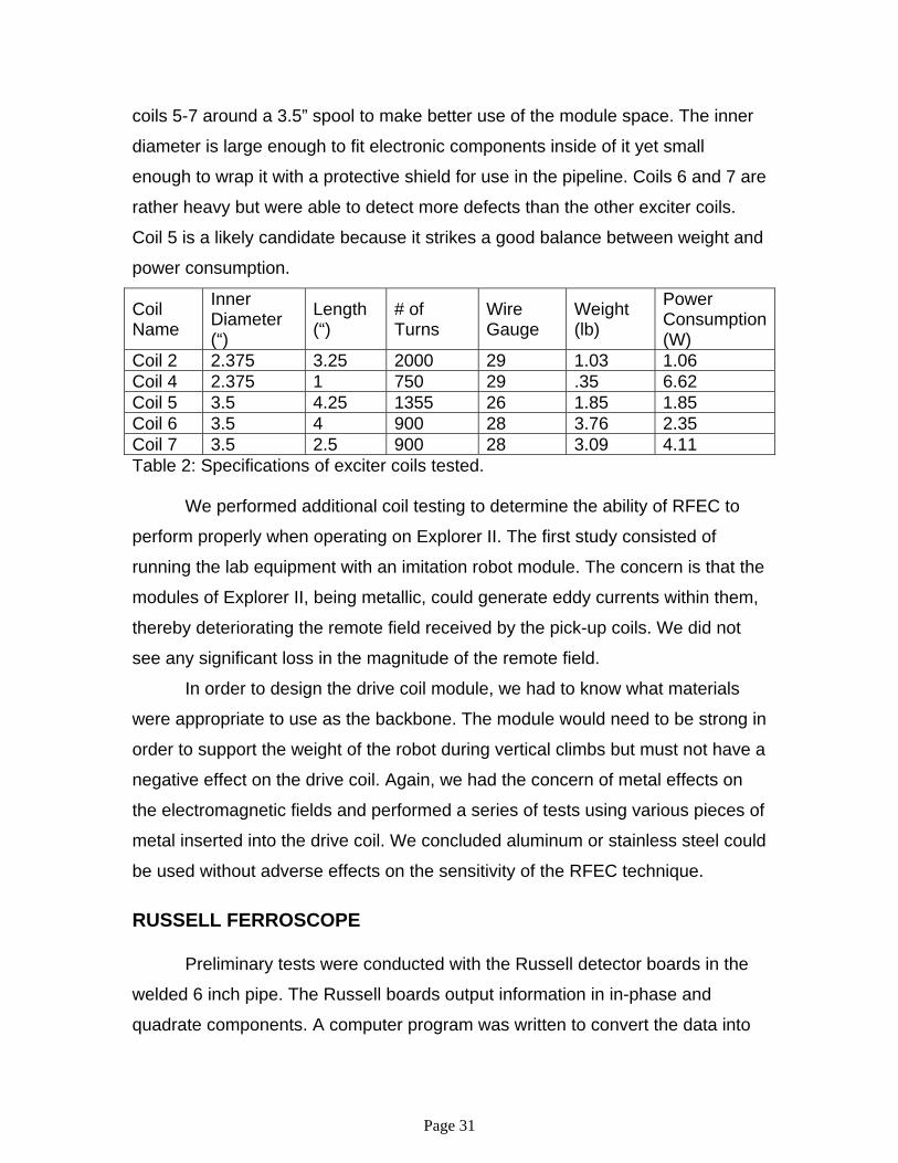
coils 5-7 around a 3.5” spool to make better use of the module space. The inner
diameter is large enough to fit electronic components inside of it yet small
enough to wrap it with a protective shield for use in the pipeline. Coils 6 and 7 are
rather heavy but were able to detect more defects than the other exciter coils.
Coil 5 is a likely candidate because it strikes a good balance between weight and
power consumption.
Coil Name
Inner Diameter (“)
Length (“)
# of Turns
Wire Gauge
Weight (lb)
Power Consumption (W)
Coil 2 2.375 3.25 2000 29 1.03 1.06 Coil 4 2.375 1 750 29 .35 6.62 Coil 5 3.5 4.25 1355 26 1.85 1.85 Coil 6 3.5 4 900 28 3.76 2.35 Coil 7 3.5 2.5 900 28 3.09 4.11 Table 2: Specifications of exciter coils tested. We performed additional coil testing to determine the ability of RFEC to
perform properly when operating on Explorer II. The first study consisted of
running the lab equipment with an imitation robot module. The concern is that the
modules of Explorer II, being metallic, could generate eddy currents within them,
thereby deteriorating the remote field received by the pick-up coils. We did not
see any significant loss in the magnitude of the remote field.
In order to design the drive coil module, we had to know what materials
were appropriate to use as the backbone. The module would need to be strong in
order to support the weight of the robot during vertical climbs but must not have a
negative effect on the drive coil. Again, we had the concern of metal effects on
the electromagnetic fields and performed a series of tests using various pieces of
metal inserted into the drive coil. We concluded aluminum or stainless steel could
be used without adverse effects on the sensitivity of the RFEC technique.
RUSSELL FERROSCOPE Preliminary tests were conducted with the Russell detector boards in the
welded 6 inch pipe. The Russell boards output information in in-phase and
quadrate components. A computer program was written to convert the data into
Page 32
amplitude and phase format for analysis. The program also allows the option to
scale the data (necessary for use in the Russell data analysis program) and to
average data over a fixed time length (useful for reducing noise levels and
comparing data with the original lock-in amplifier).
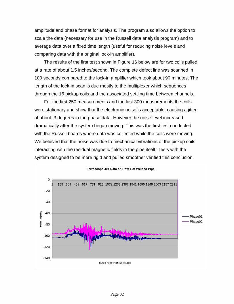
The results of the first test shown in Figure 16 below are for two coils pulled
at a rate of about 1.5 inches/second. The complete defect line was scanned in
100 seconds compared to the lock-in amplifier which took about 90 minutes. The
length of the lock-in scan is due mostly to the multiplexer which sequences
through the 16 pickup coils and the associated settling time between channels.
For the first 250 measurements and the last 300 measurements the coils
were stationary and show that the electronic noise is acceptable, causing a jitter
of about .3 degrees in the phase data. However the noise level increased
dramatically after the system began moving. This was the first test conducted
with the Russell boards where data was collected while the coils were moving.
We believed that the noise was due to mechanical vibrations of the pickup coils
interacting with the residual magnetic fields in the pipe itself. Tests with the
system designed to be more rigid and pulled smoother verified this conclusion.
Ferroscope 404 Data on Row 1 of Welded Pipe
-140
-120
-100
-80
-60
-40
-20
01 155 309 463 617 771 925 1079 1233 1387 1541 1695 1849 2003 2157 2311
Sample Number (24 samples/sec)
Phas
e (d
egre
es)
Phase01Phase02
Page 33
Figure 16: Data from defect line 1 using the Russell board.
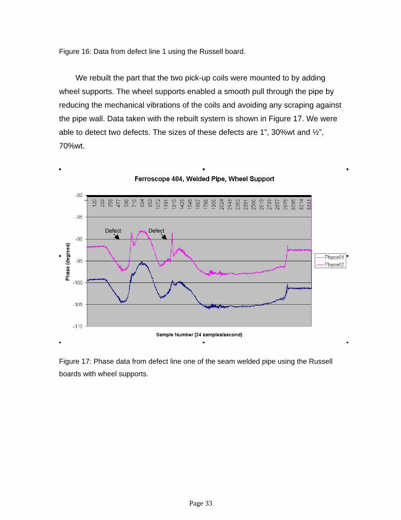
We rebuilt the part that the two pick-up coils were mounted to by adding
wheel supports. The wheel supports enabled a smooth pull through the pipe by
reducing the mechanical vibrations of the coils and avoiding any scraping against
the pipe wall. Data taken with the rebuilt system is shown in Figure 17. We were
able to detect two defects. The sizes of these defects are 1”, 30%wt and ½”,
70%wt.
Figure 17: Phase data from defect line one of the seam welded pipe using the Russell
boards with wheel supports.
Page 34
Welded Pipe, Lock-in Amplifier
0
5
10
15
20
25
20 30 40 50 60 70 80 90
Position (inches)
Phase (degrees
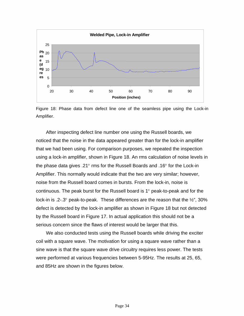
Figure 18: Phase data from defect line one of the seamless pipe using the Lock-in
Amplifier.
After inspecting defect line number one using the Russell boards, we
noticed that the noise in the data appeared greater than for the lock-in amplifier
that we had been using. For comparison purposes, we repeated the inspection
using a lock-in amplifier, shown in Figure 18. An rms calculation of noise levels in
the phase data gives .21° rms for the Russell Boards and .16° for the Lock-in
Amplifier. This normally would indicate that the two are very similar; however,
noise from the Russell board comes in bursts. From the lock-in, noise is
continuous. The peak burst for the Russell board is 1° peak-to-peak and for the
lock-in is .2-.3° peak-to-peak. These differences are the reason that the ½”, 30%
defect is detected by the lock-in amplifier as shown in Figure 18 but not detected
by the Russell board in Figure 17. In actual application this should not be a
serious concern since the flaws of interest would be larger that this.
We also conducted tests using the Russell boards while driving the exciter
coil with a square wave. The motivation for using a square wave rather than a
sine wave is that the square wave drive circuitry requires less power. The tests
were performed at various frequencies between 5-95Hz. The results at 25, 65,
and 85Hz are shown in the figures below.

Page 35
Square Drive 25 Hz
-175
-170
-165
-160
-155
-1501 42 83 124 165 206 247 288 329 370 411 452 493 534 575 616 657
Sample Number (5 samples/second)
Phas
e (d
egre
es)
Phase01Phase02
Figure 19: Phase data taken while driving the exciter coil with a 25Hz square wave.
Square Drive 65 Hz
0
5
10
15
20
25
30
35
40
45
1 40 79 118 157 196 235 274 313 352 391 430 469 508 547 586 625 664 703
Sample Number (5 samples/second)
Phas
e (d
egre
es)
Phase01Phase02
Figure 20: Phase data taken while driving the exciter coil with a 65Hz square wave.
Defects
Defects

Page 36
Square Drive 85 Hz
-70
-60
-50
-40
-30
-20
-10
01 46 91 136 181 226 271 316 361 406 451 496 541 586 631 676 721
Sample Number (5 samples/second)
Phas
e (d
egre
es)
Phase01Phase02
Figure 21: Phase data taken while driving the exciter coil with an 85Hz square wave.
Results of the 25Hz scan, shown in Figure 19, show 4 of 5 defects. Noise
levels look reasonable. Starting at 45Hz and up to 75Hz, there was quite a
disturbance in the noise. It seems to be periodic and we suspect it may be
interference from 60Hz signals created by standard electronic devices (lights,
computers, etc.) We only detected 3 of 5 defects during the 65Hz scan, shown in
Figure 20, but it is interesting to note that the amplitude of the defect signals is
considerably larger, about 3x. The amplitudes of the defect signals in the 85Hz in
Figure 21 are 4-5x larger than the signals in the 25Hz test. The periodic type
noise is reduced in the 85Hz test and 4 of 5 defects were detected.
We have observed that changes in permeability, the magnetic property of
the pipe, affect the amplitude and phase response of the RFEC. To date we rely
on the small lengths of the artificial flaws to distinguish between flaws and
permeability changes. In Figure 22 below the sharp spikes from coil 2 (Phase02)
at 121, 250, 370, and 601 are artificial flaws while the gradual peaks at 161 and
281 are permeability changes caused by residual stresses and possibly local
residual pipe magnetization. We realize that real corrosion can be much longer
Defects

Page 37
and that it may be more difficult to distinguish between them.
Scan Along Defect Line at 25 Hz
-175
-170
-165
-160
-155
-1501 41 81 121 161 201 241 281 321 361 401 441 481 521 561 601 641 681
Sample Number (5 samples/second)
Phas
e (d
egre
es)
Phase01Phase02
Figure 22: Defect scan at 25Hz
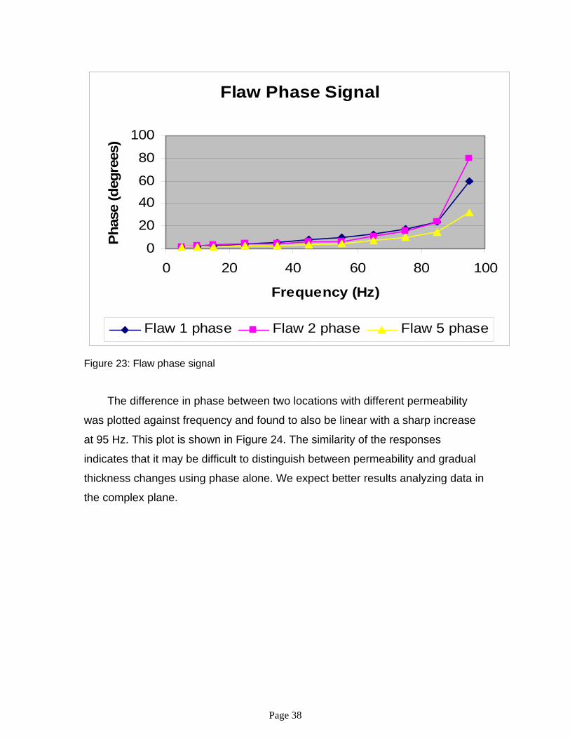
It is possible that analysis at several frequencies may help. The first step
was to look at phase information as a function of frequency. The magnitude of
the phase deviations at three artificial flaw locations was measured at different
frequencies and was found to increase linearly with frequency up to 75 Hz. The
results are shown in Figure 23. Flaw one is 1” diameter flat bottom 30% deep,
flaw two is ½” diameter round bottom 70% deep and flaw five is 1” diameter
round bottom 30% deep. There is a sharp increase at 95 Hz and then there is no
detectable flaw signal at higher frequencies. The flaws do show up in the
amplitude signal indicating that the analysis should be conducted in the complex
plane.
Page 38
Flaw Phase Signal
0
20
4060
80
100
0 20 40 60 80 100
Frequency (Hz)
Phas
e (d
egre
es)
Flaw 1 phase Flaw 2 phase Flaw 5 phase
Figure 23: Flaw phase signal
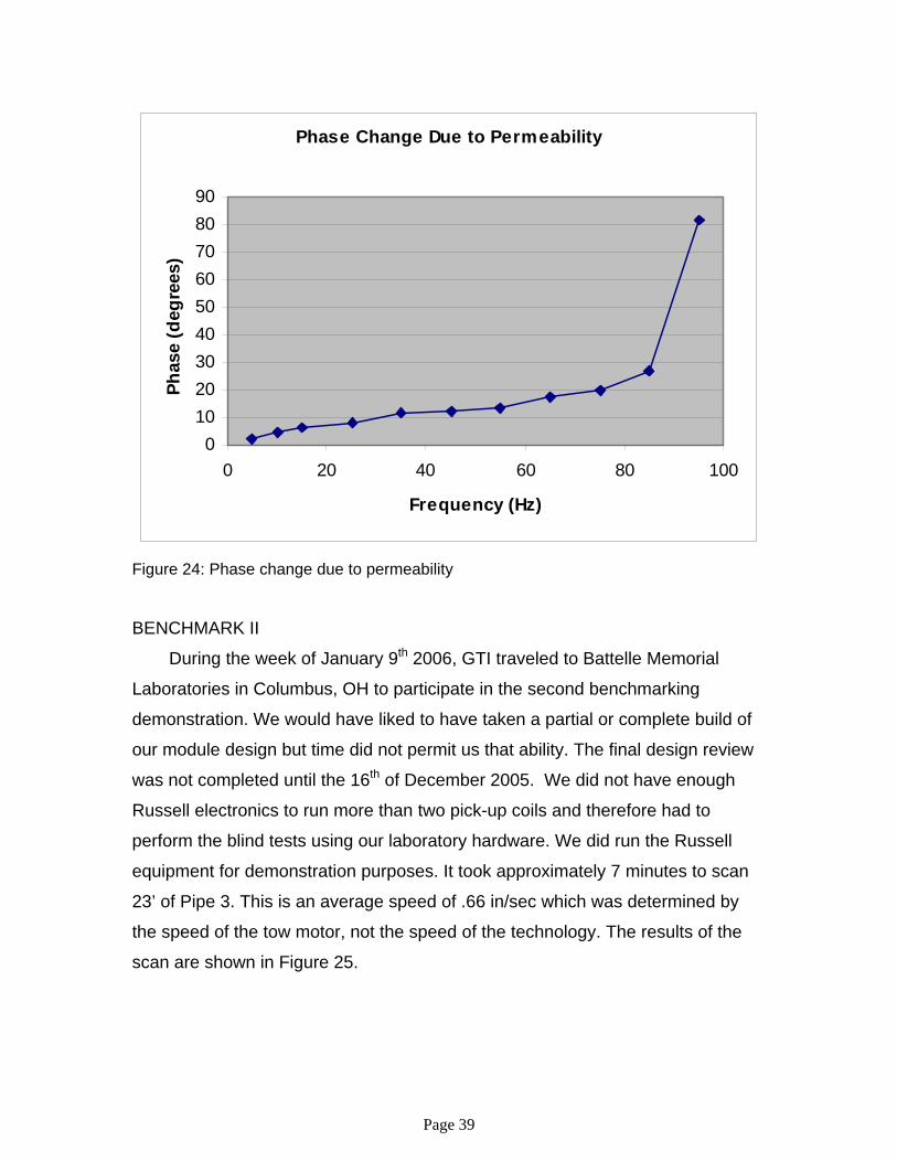
The difference in phase between two locations with different permeability
was plotted against frequency and found to also be linear with a sharp increase
at 95 Hz. This plot is shown in Figure 24. The similarity of the responses
indicates that it may be difficult to distinguish between permeability and gradual
thickness changes using phase alone. We expect better results analyzing data in
the complex plane.
Page 39
Phase Change Due to Permeability
0102030405060708090
0 20 40 60 80 100
Frequency (Hz)
Phas
e (d
egre
es)
Figure 24: Phase change due to permeability
BENCHMARK II
During the week of January 9th 2006, GTI traveled to Battelle Memorial
Laboratories in Columbus, OH to participate in the second benchmarking
demonstration. We would have liked to have taken a partial or complete build of
our module design but time did not permit us that ability. The final design review
was not completed until the 16th of December 2005. We did not have enough
Russell electronics to run more than two pick-up coils and therefore had to
perform the blind tests using our laboratory hardware. We did run the Russell
equipment for demonstration purposes. It took approximately 7 minutes to scan
23’ of Pipe 3. This is an average speed of .66 in/sec which was determined by
the speed of the tow motor, not the speed of the technology. The results of the
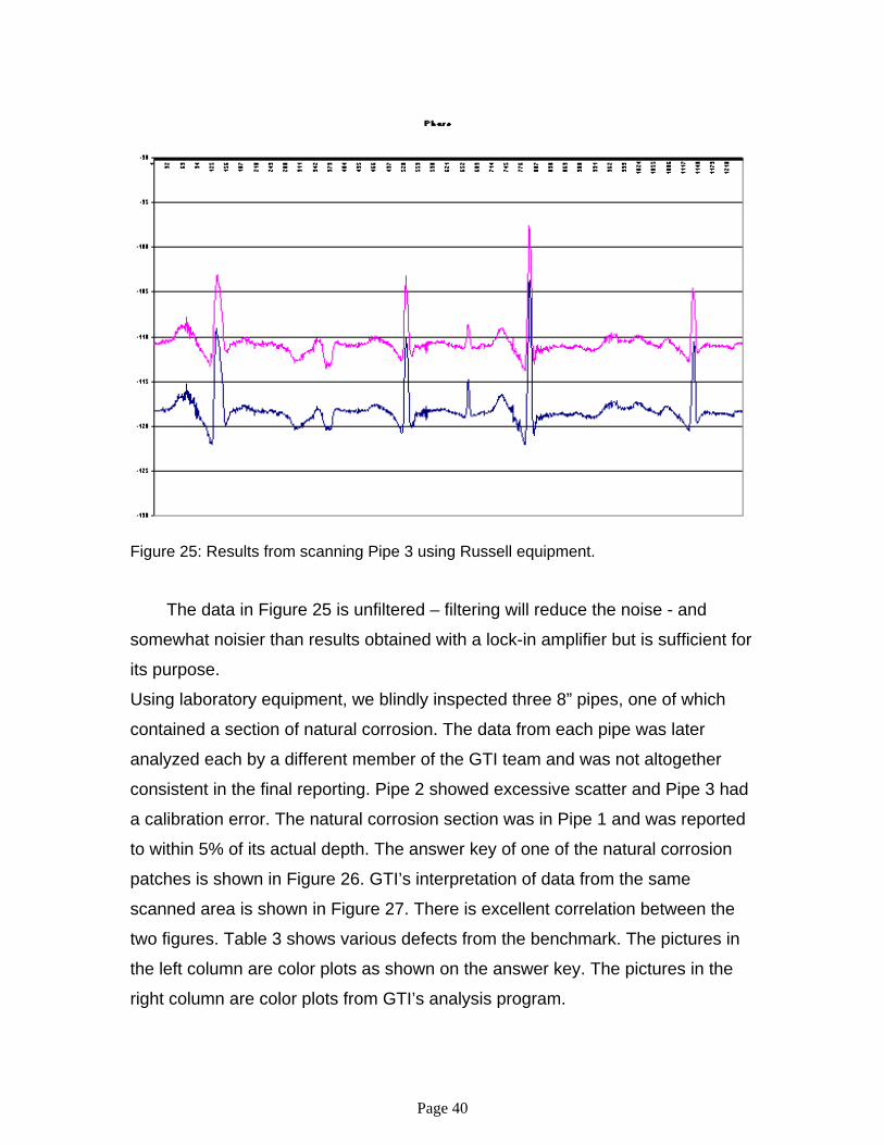
scan are shown in Figure 25.
Page 40
Figure 25: Results from scanning Pipe 3 using Russell equipment.
The data in Figure 25 is unfiltered – filtering will reduce the noise - and
somewhat noisier than results obtained with a lock-in amplifier but is sufficient for
its purpose.
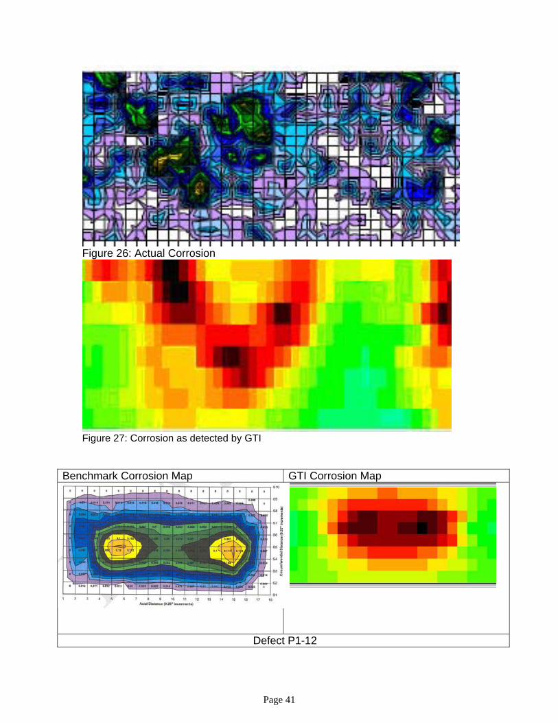
Using laboratory equipment, we blindly inspected three 8” pipes, one of which
contained a section of natural corrosion. The data from each pipe was later
analyzed each by a different member of the GTI team and was not altogether
consistent in the final reporting. Pipe 2 showed excessive scatter and Pipe 3 had
a calibration error. The natural corrosion section was in Pipe 1 and was reported
to within 5% of its actual depth. The answer key of one of the natural corrosion
patches is shown in Figure 26. GTI’s interpretation of data from the same
scanned area is shown in Figure 27. There is excellent correlation between the
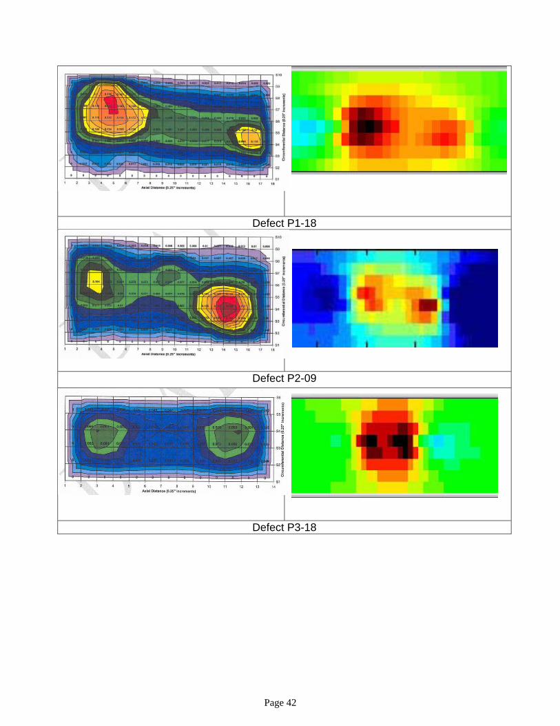
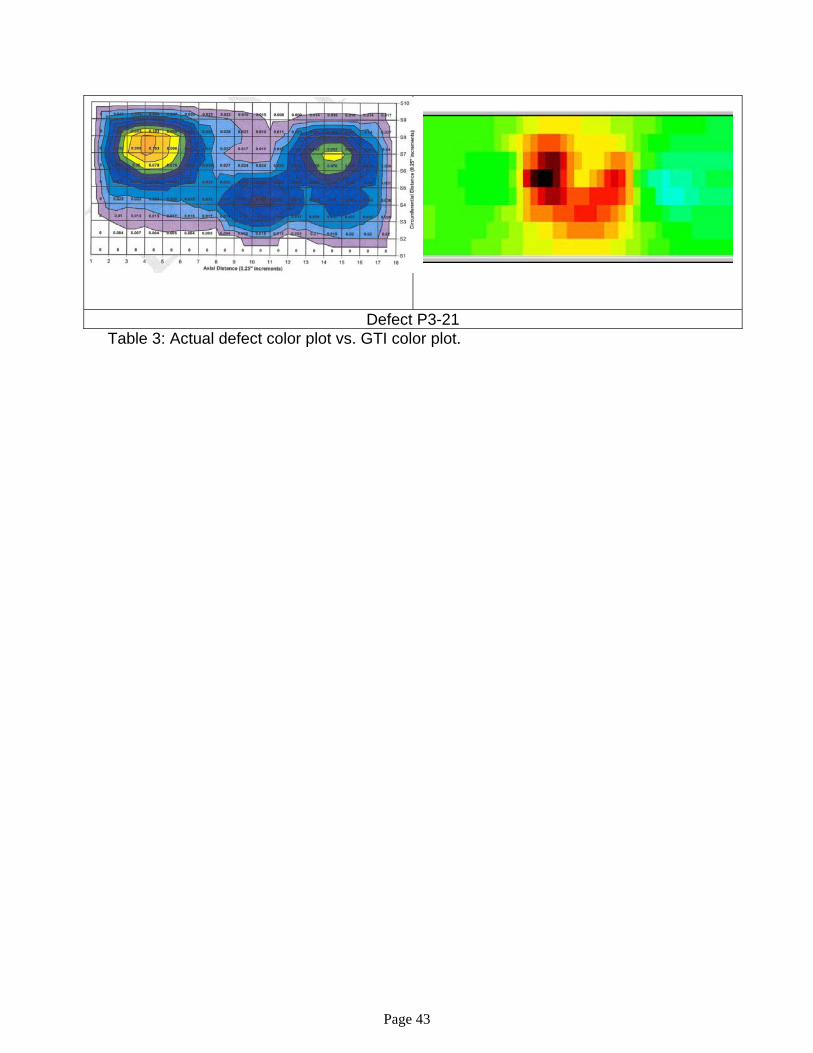
two figures. Table 3 shows various defects from the benchmark. The pictures in
the left column are color plots as shown on the answer key. The pictures in the
right column are color plots from GTI’s analysis program.
Page 41
Figure 26: Actual Corrosion
Figure 27: Corrosion as detected by GTI
Benchmark Corrosion Map GTI Corrosion Map
Defect P1-12
Page 42
Defect P1-18
Defect P2-09
Defect P3-18
Page 43
Defect P3-21 Table 3: Actual defect color plot vs. GTI color plot.
Page 44
MECHANICAL DESIGN
The design process for the pick-up coil module started early in the life of
the project. Multiple revisions were necessary. Three original designs were
created using a 3D modeling program and were presented at the mid phase
design review. One of these was chosen to go forward for the final design review.
Upon the news that DOE-NETL funding would stop at the end of Phase II due to
termination of the DOE infrastructure reliability program, GTI rescoped the work
and changed the target range from 6-8” to 10-16” pipe diameters. GTI again
revised the mechanical design.
There were certain parameters guided by the robot design and the
technology itself. Sensor coil orientation was of great importance requiring the
design to maintain the sensors parallel to pipe wall at any given diameter. For
uniformity of measurements, it was also preferred that equal distances be
maintained between the sensors. The design should also be compliant to dents,
welds, and pipe ovality, and allow the sensor to move forwards or backwards. In
order to develop a device capable of satisfying the requirements, it was found
that each sensor arm should have a single rotation point. Each progression of the
design used the radius of the module as the lever arm as opposed to lever arm
designs that would take up the length of the module and occupy space that could
otherwise be used to house electronics.
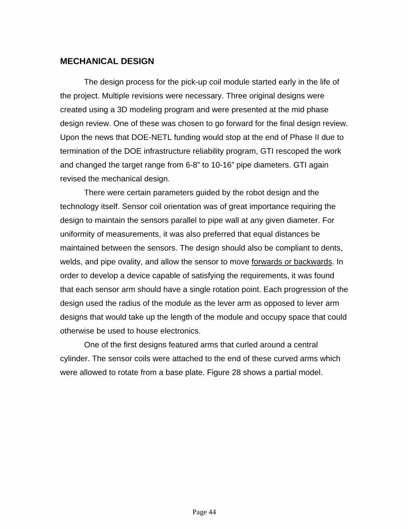
One of the first designs featured arms that curled around a central
cylinder. The sensor coils were attached to the end of these curved arms which
were allowed to rotate from a base plate. Figure 28 shows a partial model.
Page 45
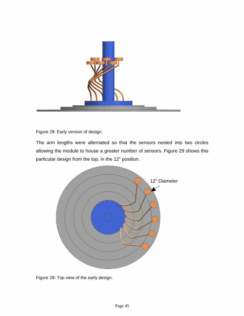
Figure 28: Early version of design. The arm lengths were alternated so that the sensors nested into two circles
allowing the module to house a greater number of sensors. Figure 29 shows this
particular design from the top, in the 12” position.
Figure 29: Top view of the early design.
12” Diameter
Page 46
The blue circle represents the base plate, which measures 4” in diameter as
required by the Explorer II specs. Each grey ring signifies and additional 2”
added to the diameter with the outermost ring being 12” in diameter. As the base
of the arms rotate in the plate, the ends of the arms are able to travel to nearly
12”.
The design evolved slightly and the arm profile was altered. The next three
figures display the changes. This version was presented at the mid phase review
meeting.
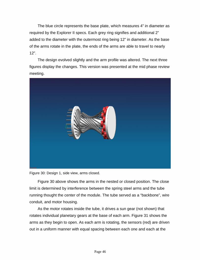
Figure 30: Design 1, side view, arms closed. Figure 30 above shows the arms in the nested or closed position. The close
limit is determined by interference between the spring steel arms and the tube
running thought the center of the module. The tube served as a “backbone”, wire
conduit, and motor housing.
As the motor rotates inside the tube, it drives a sun gear (not shown) that
rotates individual planetary gears at the base of each arm. Figure 31 shows the
arms as they begin to open. As each arm is rotating, the sensors (red) are driven
out in a uniform manner with equal spacing between each one and each at the

Page 47
same distance from the center. The fully extended position is shown in Figure 32.
Figure 31: Design 1, side view, arms partially open.
Figure 32: Design 1, side view, arms completely open.

Page 48
The problems we encountered with the previously shown module were the
lack of available space for electronics and complexity of manufacture. The swing
of the arms required so much module space remain vacant that there was little
room left for electronics. Each individual arm required precise construction which
would have driven the building costs too high.
The next evolution of the module design featured electronics boards as the
arms. This concept decreased the overall length by 30% and incorporated the
electronics in the arms. A 2-D sketch of this design is shown in Figure 33 to
portray the compactness of the design.
Figure 33: Design 2, 2-D sketch, side view.
Page 49
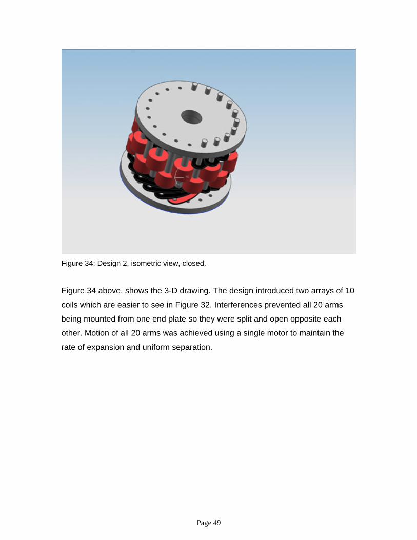
Figure 34: Design 2, isometric view, closed.
Figure 34 above, shows the 3-D drawing. The design introduced two arrays of 10
coils which are easier to see in Figure 32. Interferences prevented all 20 arms
being mounted from one end plate so they were split and open opposite each
other. Motion of all 20 arms was achieved using a single motor to maintain the
rate of expansion and uniform separation.

Page 50
Figure 35: Design 2, isometric view, partially open.
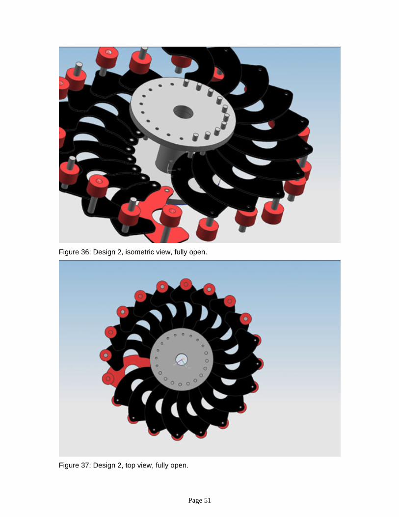
The shape of the arms were a result of the design itself. Although the face
area was made as large as possible, provisions had to be made for the center
rod of the module. Additionally, the overlap seen by each arm at full extension
prevents them from slipping past one another ensuring the arms will be able to
be retracted. This feature is evident in the next two figures. Figure 36 give a good
indication of the separation between each set of arms. This separation, although
forced by the design, helps reduce the amount of gas flow blockage. Even if
there were not an axial spacing between the arrays, the module would create no
more blockage than an orifice meter. Figure 37 shows the uniform spacing of the
sensors.
Page 51
Figure 36: Design 2, isometric view, fully open.
Figure 37: Design 2, top view, fully open.
Page 52
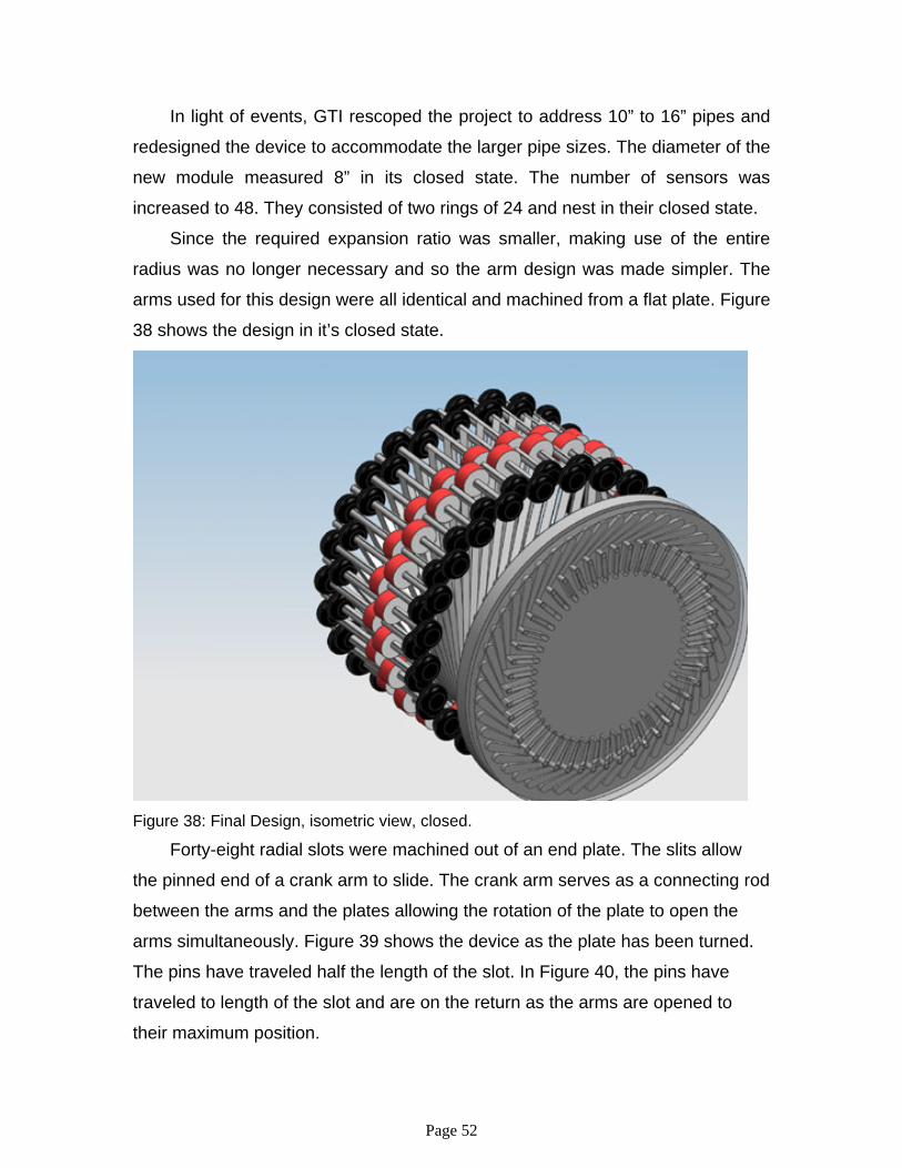
In light of events, GTI rescoped the project to address 10” to 16” pipes and
redesigned the device to accommodate the larger pipe sizes. The diameter of the
new module measured 8” in its closed state. The number of sensors was
increased to 48. They consisted of two rings of 24 and nest in their closed state.
Since the required expansion ratio was smaller, making use of the entire
radius was no longer necessary and so the arm design was made simpler. The
arms used for this design were all identical and machined from a flat plate. Figure
38 shows the design in it’s closed state.
Figure 38: Final Design, isometric view, closed.
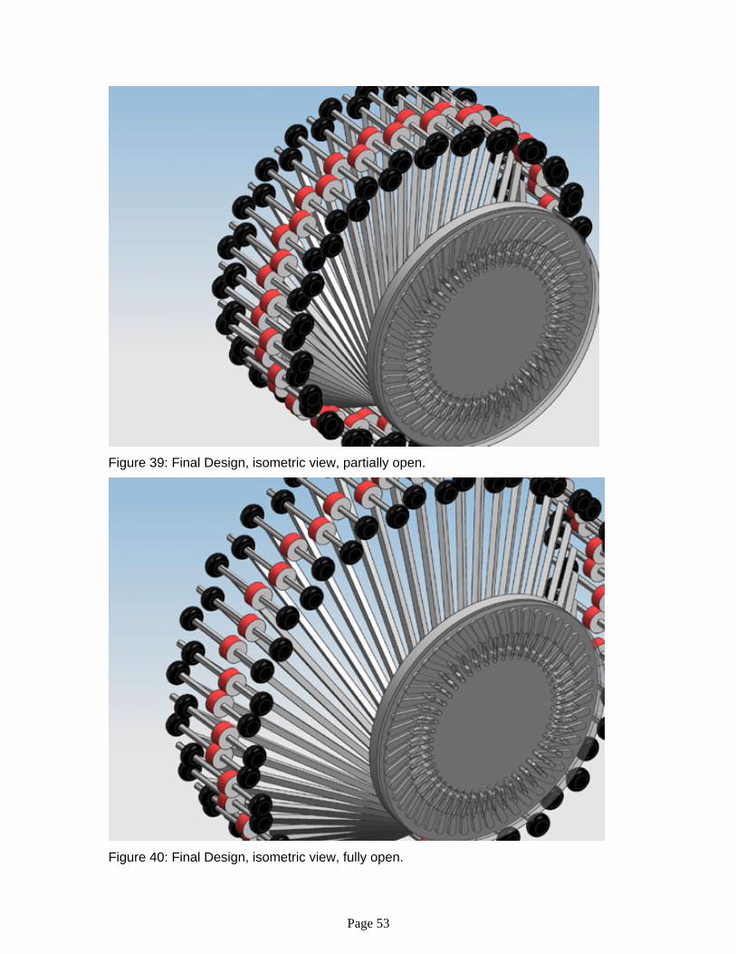
Forty-eight radial slots were machined out of an end plate. The slits allow
the pinned end of a crank arm to slide. The crank arm serves as a connecting rod
between the arms and the plates allowing the rotation of the plate to open the
arms simultaneously. Figure 39 shows the device as the plate has been turned.
The pins have traveled half the length of the slot. In Figure 40, the pins have
traveled to length of the slot and are on the return as the arms are opened to
their maximum position.
Page 53
Figure 39: Final Design, isometric view, partially open.
Figure 40: Final Design, isometric view, fully open.
Page 54
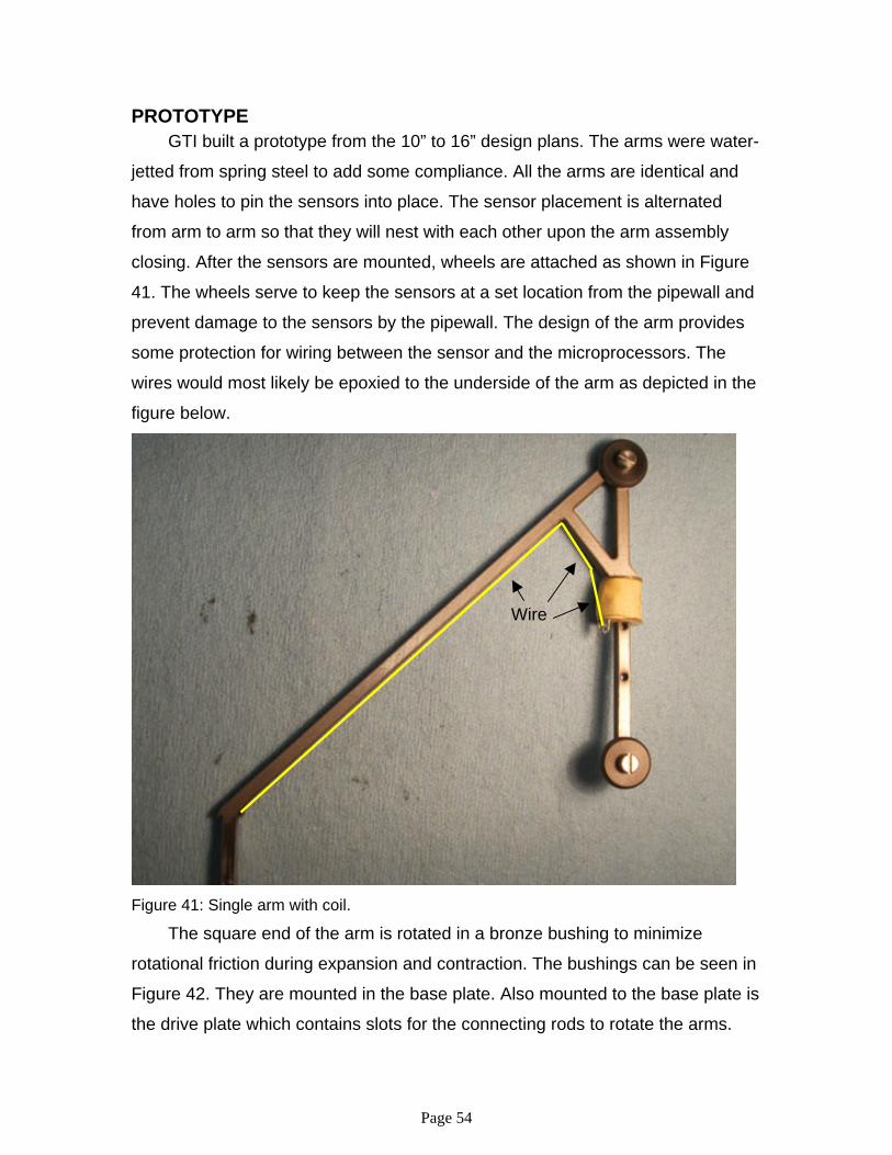
PROTOTYPE GTI built a prototype from the 10” to 16” design plans. The arms were water-
jetted from spring steel to add some compliance. All the arms are identical and
have holes to pin the sensors into place. The sensor placement is alternated
from arm to arm so that they will nest with each other upon the arm assembly
closing. After the sensors are mounted, wheels are attached as shown in Figure
41. The wheels serve to keep the sensors at a set location from the pipewall and
prevent damage to the sensors by the pipewall. The design of the arm provides
some protection for wiring between the sensor and the microprocessors. The
wires would most likely be epoxied to the underside of the arm as depicted in the
figure below.
Figure 41: Single arm with coil. The square end of the arm is rotated in a bronze bushing to minimize
rotational friction during expansion and contraction. The bushings can be seen in
Figure 42. They are mounted in the base plate. Also mounted to the base plate is
the drive plate which contains slots for the connecting rods to rotate the arms.
Wire

Page 55
There is a ring mounted to the drive plate. The drive plate is allowed to rotate
approximately 35° and is contained by bushings in slots on the ring.
Figure 42: Base plate, pre-mounting. Motion is accomplished by gearing. The ring has teeth machined into the
inside diameter. The motor and the gear mounted to it are shown in Figure 42 at
the top, center position. When the gear turns, it drives the ring and drive plate.
The drive plate’s motion causes the pins on the crank arm to travel which causes
the arms to turn.
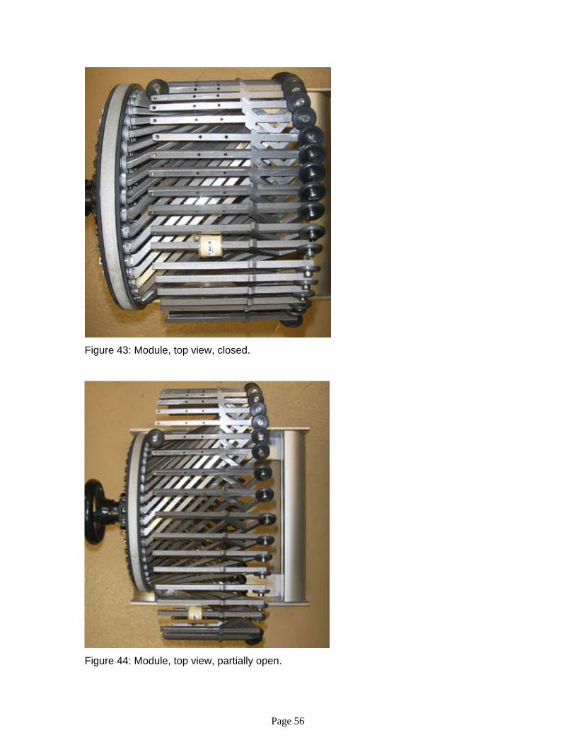
Figure 43 shows the module after the arms have been installed. Only one
coil was mounted. The module is shown in its closed position. The diameter of
the module is 7 – ¾” allowing it to pass through an 8” entrance.
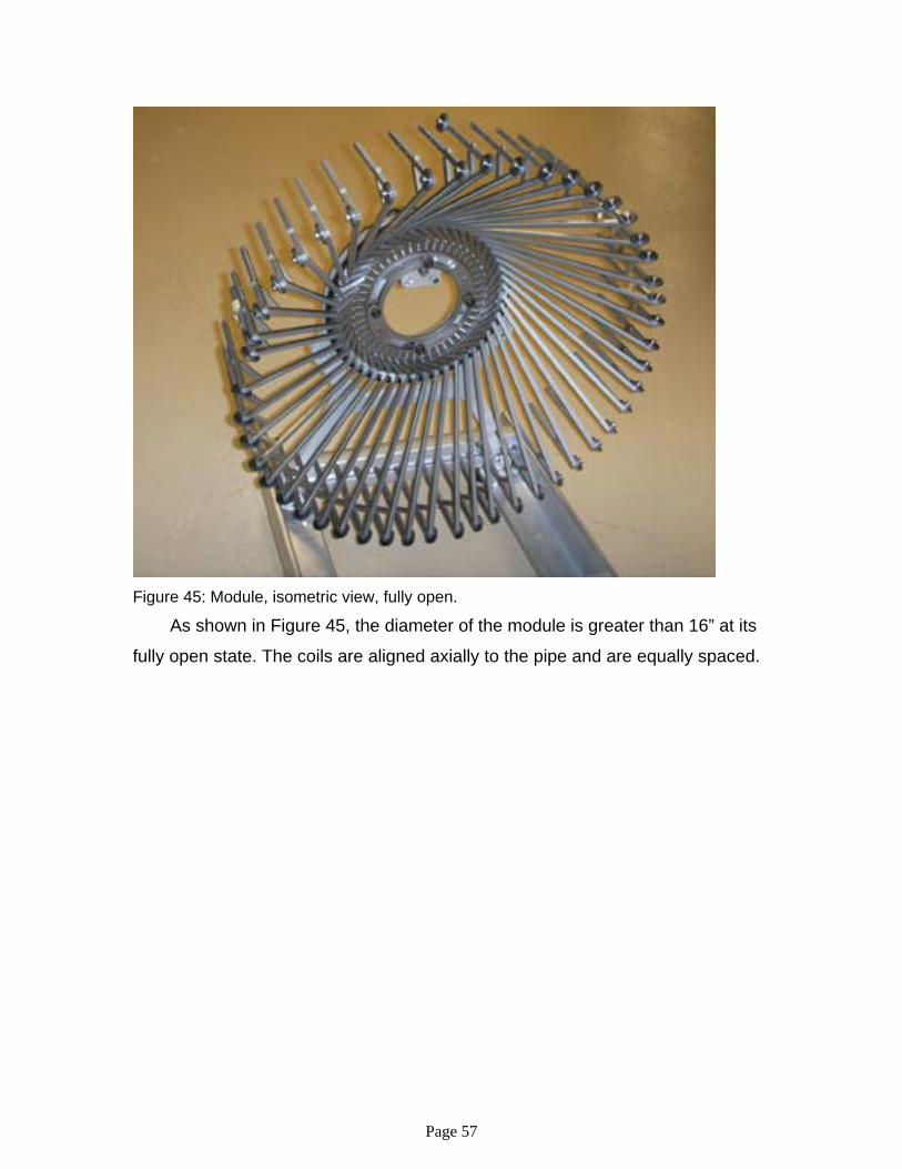
Figure 44 shows the module as the arms have opened part of the way.
Note the amount of travel of the arm with the sensor.
Page 56
Figure 43: Module, top view, closed.
Figure 44: Module, top view, partially open.
Page 57
Figure 45: Module, isometric view, fully open. As shown in Figure 45, the diameter of the module is greater than 16” at its
fully open state. The coils are aligned axially to the pipe and are equally spaced.

Page 58
ELECTRONIC DESIGN AND IMPLIMENTATION
The data collection and electronics are controlled by a master PIC16F87
microprocessor that provides the magic sinewave data used to generate the
drive coil signal and the slave PIC16C773 microprocessors that convert the
output of the sensor amplifiers to a digital value and store it in 24LC256 256KB
memory chips.
The block diagram is shown in Figure 46. The master generates the magic
sinewave sequences and outputs them to the S↑ and S↓ pins. One op amp
inverts the S↓ signal, while a second integrates the summed bit streams and
outputs the resulting sine wave to a potentiometer. An inverting op amp and a
non-inverting op amp amplify the sine wave and drive the exciter coil that
generates the RFEC electromagnetic waves. High gain, low noise, op amps
amplify the output from the sensing coils, located about 2 pipe diameters from
the drive coil, and input the signal to the 12 bit ADCs of the slave
microprocessors. The output of each ADC is stored in a 256 KB memory chip
and can also be transmitted to an RS232 interface for monitoring by the operator
at the end of the tether. The master processor can also be controlled and
reprogrammed through this interface.
Information on magic sinewaves can be found on the internet,
http://www.tinaja.com/magsn01.asp . They consist of carefully selected
sequences of ones and zeros, easily generated by a microprocessor that can
then be integrated to generate sine waves with an arbitrary number of lower
harmonics forced precisely to zero.
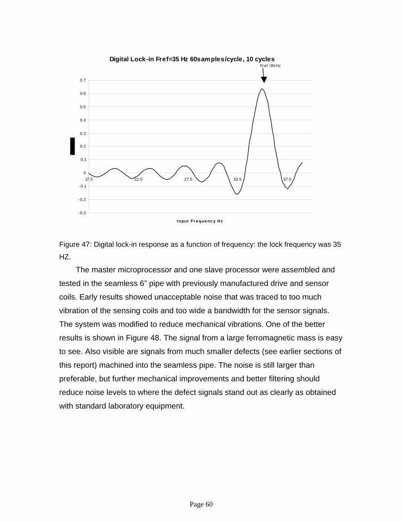
Digital lock-in amplifiers, programmed into the slave processors, are used to
filter the input signals from the sensors. The method basically consists of
summing the amplified sensor signals into In-Phase and Quadrature-Phase bins
for a programmable number of cycles. Figure 47 shows the frequency response
to sine waves from 17.5 Hz to about 40 Hz for a digital lock-in with a 35 HZ lock
frequency integrated over 10 cycles.

Page 59
Figure 46: Block diagram of the electronic components.
Page 60
Digital Lock-in Fref=35 Hz 60samples/cycle, 10 cycles
-0.3
-0.2
-0.1
0
0.1
0.2
0.3
0.4
0.5
0.6
0.7
17.5 22.5 27.5 32.5 37.5
I nput Fr e que nc y Hz
Fref =35 Hz
Figure 47: Digital lock-in response as a function of frequency: the lock frequency was 35
HZ.
The master microprocessor and one slave processor were assembled and
tested in the seamless 6” pipe with previously manufactured drive and sensor
coils. Early results showed unacceptable noise that was traced to too much
vibration of the sensing coils and too wide a bandwidth for the sensor signals.
The system was modified to reduce mechanical vibrations. One of the better
results is shown in Figure 48. The signal from a large ferromagnetic mass is easy
to see. Also visible are signals from much smaller defects (see earlier sections of
this report) machined into the seamless pipe. The noise is still larger than
preferable, but further mechanical improvements and better filtering should
reduce noise levels to where the defect signals stand out as clearly as obtained
with standard laboratory equipment.

Page 61
xlabb2 d=20 g=248
-50
0
50
100
150
200
250
180 280 380 480 580 680
20
30
40
50
60
70
80
Amp Phase
Figure 48: A test run of the electronic assembly using a master and one slave
microprocessor programmed with a digital lock-in amplifier.
The electronic design for 10” to 16” pipe calls for collecting the information
from 48 or more sensors. The existing electronics contains only one slave
microprocessor, while the present design calls for one slave processor per coil.
For the data to be available real time to the operator of the RFEC inspection unit,
the results of all 48 processors need to be sent along the tether. This requires
some form of multiplexing. Several schemes are under consideration. These
involve one or more master processors to manage the memories and transmit
the data to the operator. For example, the memory chip selected can has 8
addresses. To address all 48 channels would therefore require 6 groups of 8
each with its own PIC. An alternative scheme would dump all the data to an SD
card that could then be read by the operator’s PC. A final decision has not been
made and implementation will require additional resources.
Page 62
CONCLUSION
Although we are disappointed that the ultimate objective of this project
was not reached, at this time, due to issues related to funding, we are still
pleased with the quality of research that was accomplished. Improvements in the
laboratory setup which include automation of the equipment, allowed us to
perform a large variety of tests. We tested seven exciter coils and gained
valuable knowledge about coil geometry’s effect on the magnitude of the
electromagnetic field. We were able to improve the sensitivity of the sensor coils
and detect 5% wt defects, all the while requiring less power than would be
available on an autonomous robot. We also tested commercial electronics from
Russell Technologies and built and tested our own electronics.
Multiple preliminary module designs were drafted using 3D modeling
software. One of these designs evolved into a final design that is currently under
review for patent. This innovative design was capable of traversing pipe in two
directions. With the decision to not integrate GTI’s sensors with a robot, the
design was resized for 10” to 16” pipe diameters, targeted for tethered platforms,
and was built.
Page 63
REFERENCES W.R. McLean, W. R., US Patent 2,573,799, “Apparatus for Magnetically Measuring Thickness of Ferrous Pipe”, Nov. 6, 1951 Schmidt, T. R., “The Casing Instrument Tool-…”, Corrosion, pp 81-85, July 1961 Atherton, D. L., US patent 6,127,823, “Electromagnetic Method for Non-Destructive Testing of Prestressed Concrete Pipes for Broken Prestressed Wires”, Oct. 3, 2000
Takach, S. F., Teitsma, A., Maupin, J., Seger, P., and Shuttleworth, P. “Remote Field Eddy Current Inspection for Unpiggable Pipelines” Proc. Of Natural Gas Technologies 2005, GTI-04/0252, Gas Technology Institute, 2005 Maupin J., Teitsma, A., “Delivery Reliability for Natural Gas -- Inspection Technologies Phase I Topical Report” October 2005
Teitsma, A., et al. “Small Diameter Remote Field Eddy Current Inspection of Unpiggable Pipelines” Journal of Pressure Vessel Technology, 2005
Page 64
TABLE OF FIGURES Figure 1: Variation of the amplitude of propagating fields with distance along a pipe. ......................................................................................................................6 Figure 2: A simulated drawing of the RFEC technology integrated with Explorer. 7 Figure 3: RFEC laboratory setup. .......................................................................10 Figure 4: The logarithm of the dipole moment as a function of the number of turns and the relative permeability. ..............................................................................14 Figure 5: The FEA model of the 6” x 0.25” seamless pipe, showing lines of magnetic flux density. .........................................................................................16 Figure 6: Robot modules attenuate the direct field more rapidly. ........................17 Figure 7: Screen shot of 6” seamless pipe scan from Adept Pro Software. ........18 Figure 8: Screen shot of 6” lined Cast Iron. ........................................................20 Figure 9: Results of scanning the 6” seamless pipe with differential coils...........21 Figure 10: Results of 6” seamless pipe scan using Coil 5 with a mock module. .23 Figure 11: Results of a pullout test using Coil 6. .................................................24 Figure 12: Results of scanning the 6” seamless pipe with Coil 6. .......................25 Figure 13: Results of a pullout test using Coil 7. .................................................26 Figure 14: Results of scanning the 6” seamless pipe with Coil 7. .......................27 Figure 15: Results of scanning the 6” welded pipe with Coil 7............................29 Figure 16: Data from defect line 1 using the Russell board. ...............................33 Figure 17: Phase data from defect line one of the seam welded pipe using the Russell boards with wheel supports....................................................................33 Figure 18: Phase data from defect line one of the seamless pipe using the Lock-in Amplifier. .........................................................................................................34 Figure 19: Phase data taken while driving the exciter coil with a 25Hz square wave. ..................................................................................................................35 Figure 20: Phase data taken while driving the exciter coil with a 65Hz square wave. ..................................................................................................................35 Figure 21: Phase data taken while driving the exciter coil with an 85Hz square wave. ..................................................................................................................36 Figure 22: Defect scan at 25Hz ..........................................................................37 Figure 23: Flaw phase signal ..............................................................................38 Figure 24: Phase change due to permeability.....................................................39 Figure 25: Results from scanning Pipe 3 using Russell equipment. ...................40 Figure 26: Actual Corrosion ................................................................................41 Figure 27: Corrosion as detected by GTI ............................................................41 Figure 28: Early version of design.......................................................................45 Figure 29: Top view of the early design. .............................................................45 Figure 30: Design 1, side view, arms closed.......................................................46 Figure 31: Design 1, side view, arms partially open............................................47 Figure 32: Design 1, side view, arms completely open. ......................................47 Figure 33: Design 2, 2-D sketch, side view.........................................................48 Figure 34: Design 2, isometric view, closed........................................................49 Figure 35: Design 2, isometric view, partially open. ............................................50 Figure 36: Design 2, isometric view, fully open. ..................................................51
Page 65
Figure 37: Design 2, top view, fully open. ...........................................................51 Figure 38: Final Design, isometric view, closed. .................................................52 Figure 39: Final Design, isometric view, partially open. ......................................53 Figure 40: Final Design, isometric view, fully open. ............................................53 Figure 41: Single arm with coil. ...........................................................................54 Figure 42: Base plate, pre-mounting...................................................................55 Figure 43: Module, top view, closed....................................................................56 Figure 44: Module, top view, partially open.........................................................56 Figure 45: Module, isometric view, fully open. ....................................................57 Figure 46: Block diagram of the electronic components. ....................................59 Figure 47: Digital lock-in response as a function of frequency: the lock frequency was 35 HZ...........................................................................................................60 Figure 48: A test run of the electronic assembly using a master and one slave microprocessor programmed with a digital lock-in amplifier................................61

Page 66
LIST OF ACRONYMS AND ABBREVIATIONS RFEC Remote Field Eddy Current GTI Gas Technology Institute BOP Bipolar Operational Amplifier V rms Volts root mean square A rms Amps root mean square mV Millivolt W Watt UML Unified Modeling Language MFL Magnetic Flux Leakage DOE Department of Energy NETL National Energy Technology Laboratory wt Wall Thickness Hz Hertz CMU Carnegie Mellon University