reduced order modeling of floating offshore wind … · how to reduce/simplify the model? 4....
TRANSCRIPT

Stuttgart Wind Energy @ Institute of Aircraft Design
Reduced Order Modeling of Floating Offshore Wind Turbines
2nd International Summer School on Stochastic Dynamics of Wind Turbines and Wave Energy Absorbers August, 6th - 8th, 2014
Aalborg University
Frank Sandner, Stuttgart Wind Energy (SWE) University of Stuttgart/Germany
2 | (58)
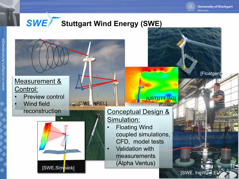
Stuttgart Wind Energy (SWE)
Measurement & Control: • Preview control • Wind field
reconstruction Conceptual Design & Simulation: • Floating Wind
coupled simulations, CFD, model tests
• Validation with measurements (Alpha Ventus)
[Floatgen]
[SWE, InnWind.EU] [SWE,Simpack]
[SWE, NREL] [USTUTT,IAG]

Stuttgart Wind Energy @ Institute of Aircraft Design
Acknowledgements
The use and re-distribution of the slides is only allowed upon request to the author.
These slides are partly based on work by Denis Matha, Steffen Raach and David Schlipf. Their contribution is greatly appreciated.

4 | (58)
What‘s in this lecture?
• To get an understanding of the Floating Wind Turbine (FOWT) as a dynamic system and its modeling techniques.
• To get an idea of how to select the appropriate model simplification.
• To set up a first „coupled“ model.
5 | (58)
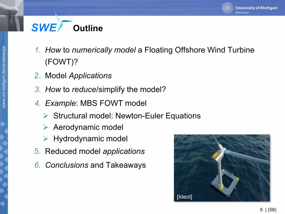
Outline
1. How to numerically model a Floating Offshore Wind Turbine (FOWT)?
2. Model Applications
3. How to reduce/simplify the model?
4. Example: MBS FOWT model Structural model: Newton-Euler Equations Aerodynamic model Hydrodynamic model
5. Reduced model applications
6. Conclusions and Takeaways
[Ideol]

6 | (58)
How to model a FOWT (in general)? (1)

7 | (58)
How to model a FOWT (in general)? (2)
Model features:
• Coupled/uncoupled • Static/dynamic • Linear/nonlinear • Steady/transient • Time/frequency domain • Frequency range • DOFs, involved modes • 2D/3D • Parametrizable • Computational effort/speed
(real-time?)
8 | (58)
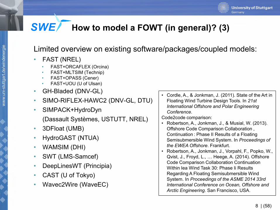
How to model a FOWT (in general)? (3) Limited overview on existing software/packages/coupled models:
• FAST (NREL) • FAST+ORCAFLEX (Orcina) • FAST+MLTSIM (Technip) • FAST+OPASS (Cener) • FAST+UOU (U of Ulsan)
• GH-Bladed (DNV-GL) • SIMO-RIFLEX-HAWC2 (DNV-GL, DTU) • SIMPACK+HydroDyn
(Dassault Systèmes, USTUTT, NREL) • 3DFloat (UMB) • HydroGAST (NTUA) • WAMSIM (DHI) • SWT (LMS-Samcef) • DeepLinesWT (Principia) • CAST (U of Tokyo) • Wavec2Wire (WaveEC)
• Cordle, A., & Jonkman, J. (2011). State of the Art in Floating Wind Turbine Design Tools. In 21st International Offshore and Polar Engineering Conference.
Code2code comparison: • Robertson, A., Jonkman, J., & Musial, W. (2013).
Offshore Code Comparison Collaboration , Continuation : Phase II Results of a Floating Semisubmersible Wind System. In Proceedings of the EWEA Offshore. Frankfurt.
• Robertson, A., Jonkman, J., Vorpahl, F., Popko, W., Qvist, J., Froyd, L., … Heege, A. (2014). Offshore Code Comparison Collaboration Continuation Within Iea Wind Task 30: Phase Ii Results Regarding A Floating Semisubmersible Wind System. In Proceedings of the ASME 2014 33rd International Conference on Ocean, Offshore and Arctic Engineering. San Francisco, USA.

9 | (58)
Model Applications (1)
• Overview on model applications
Why do we need reduced/simplified models?

11 | (58)
Model Applications (2)
1. Conceptual design: • Early stage coupled simulations • Parametric studies • Fast load simulations
[Ideol]
DLC
Wind Conditions Wave Conditions
Events PSF Model Wind Speed Model Wave Height Direction
1.x Power Production
1.1 NTM Vin < VHub < VOut NSS Hs = E[Hs | VHub] β = 0° Normal operation 1.25 ∙ 1.2
1.3 ETM Vin < VHub < VOut NSS Hs = E[Hs | VHub] β = 0° Normal operation 1.35
1.4 ECD Vhub=Vr+/- 2m/s, Vout NSS Hs = E[Hs | VHub] β = 0° Normal operation 1.35
1.5 EWS Vin < VHub < VOut NSS Hs = E[Hs | VHub] β = 0° Normal operation 1.35
1.6a NTM Vin < VHub < VOut ESS Hs = 1.09 ∙ Hs50 β = 0° Normal operation 1.35
2.x Power production plus occurrence of fault
2.1 NTM Vhub=Vr , VOut NSS Hs = E[Hs | VHub] β = 0° Pitch runaway 1.35
2.3 EOG Vhub=Vr+/- 2m/s, VOut NSS Hs = E[Hs | VHub] β = 0° Loss of load 1.1
6.x Parked (standing still or idling)
6.1a EWM VHub = 0.95 ∙ V50 ESS Hs = 1.09 ∙ Hs50 β = 0°, ± 30° Yaw = 0°, ± 8° 1.35
6.2a* EWM VHub = 0.95 ∙ V50 ESS Hs = 1.09 ∙ Hs50 β = 0°, ± 30° -180° < Yaw < 180° 1.1
6.3a EWM VHub = 0.95 ∙ V1 ESS Hs = 1.09 ∙ Hs1 β = 0°, ± 30° Yaw = 0°, ± 20° 1.35
7.x Parked and fault condition
7.1a EWM VHub = 0.95 ∙ V1 ESS Hs = 1.09 ∙ Hs1 β = 0°, ± 30° Yaw = 0°, ± 8°
1 seized blade 1.1

12 | (58)
Model Applications (3)
1. Conceptual design: • Early stage coupled dynamic simulations • Parametric studies • Fast load simulations
2. Study/understanding of system dynamics:
13 | (58)
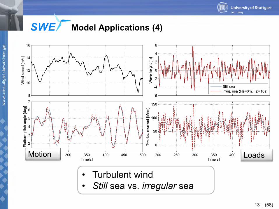
Model Applications (4)
• Turbulent wind • Still sea vs. irregular sea
Motion Loads

14 | (58)
Model Applications (5)
1. Conceptual design: • Early stage coupled dynamic simulations • Parametric studies • Fast load simulations
2. Study/understanding of system dynamics: • Controller design • Mass dampers • Subsystem adaptation (mooring lines,
secondary elements)
[Stewart 2012]
15 | (58)
Model Applications (6)
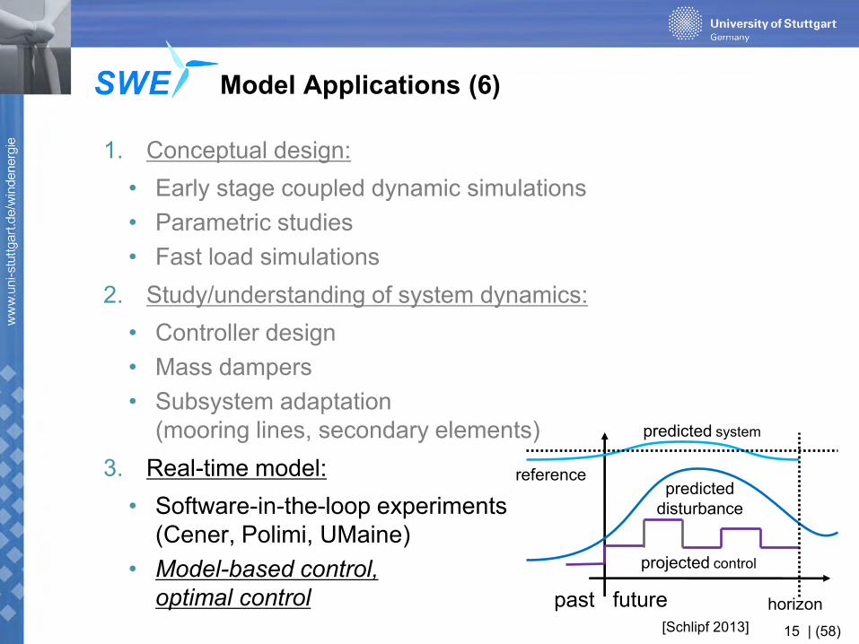
1. Conceptual design: • Early stage coupled dynamic simulations • Parametric studies • Fast load simulations
2. Study/understanding of system dynamics: • Controller design • Mass dampers • Subsystem adaptation
(mooring lines, secondary elements) 3. Real-time model:
• Software-in-the-loop experiments (Cener, Polimi, UMaine)
• Model-based control, optimal control
past
predicted disturbance
predicted system
reference
future
projected control
horizon [Schlipf 2013]

16 | (58)
Model Applications: Summary
Questions to be answered by the model:
1. System dynamics or component dynamics (specific effect)?
2. Coupled or uncoupled dynamics?
3. Type of analysis: Steady states, modal, or frequency reponse?
4. Outputs: Displacements, sectional loads, stresses
5. Postprocessing: Min/Max/Mean/Stdev, etc.
Constraints:
1. Availability of data
2. Computational speed
3. Parametrization, batch mode
4. „Flexibility“ of the software, availability of the code

17 | (58)
How to „reduce“ the FOWT model? (1)
Structural Model:
EMBS
• Elastic Multibody system (EMBS) • Elastic parts: full FEM or reduced
MBS
• MBS of rigid bodies • Spring-damper couplings
Reduction
• Modal reduction, CMS (e.g. Craig Bampton Method)
• Krylov subspace, SVD

18 | (58)
How to „reduce“ the FOWT model? (2)
EMBS reduction: Project the equations of motion into a „smaller space“.
• Modal approximation: Spatial loads not considered. • Guyan reduction (condensation): Separation of
Master (external, interface) and Slave (internal, node displacement) coordinates.
• Component mode synthesis (CMS): Identification of „component modes“. Homogeneous and particular solution to the EQM „correction modes“.
• Krylov subspace methods: Large sparse systems, TF estimation
• Singular value decomposition (SVD): Energy consideration, identification of system invariants.
„traditional techniques“
„modern techniques“
Nowakowski, C., Fehr, J., Fischer, M., & Eberhard, P. (2012). Model Order Reduction in Elastic Multibody Systems using the Floating Frame of Reference Formulation. In MATHMOD. Retrieved from http://seth.asc.tuwien.ac.at/proc12/full_paper/Contribution475.pdf
Stru
ctur
al d
ynam
ics

19 | (58)
Ab = 0.9969 -0.0030 0.0008 -0.0007 -0.0000 -0.0018 0.9801 0.0105 -0.0090 -0.0005 -0.0005 0.0013 0.9899 0.0177 0.0009 -0.0002 0.0058 -0.0162 0.8036 -0.0241 -0.0000 -0.0005 -0.0005 0.0033 0.9913
How to „reduce“ the FOWT model? (3)
Singular-value decomposition (SVD):
Bb = -0.1445 -0.0246 -0.0537 0.0488 -0.0090 -0.0175 -0.0008 -0.0165 -0.0011 0.0001
Cb = -0.1466 -0.0725 0.0192 -0.0162 -0.0009
A2 B2
C2
[Lecture Notes Kenn Oldham, Umich ME562 2010]
Stru
ctur
al d
ynam
ics
20 | (58)
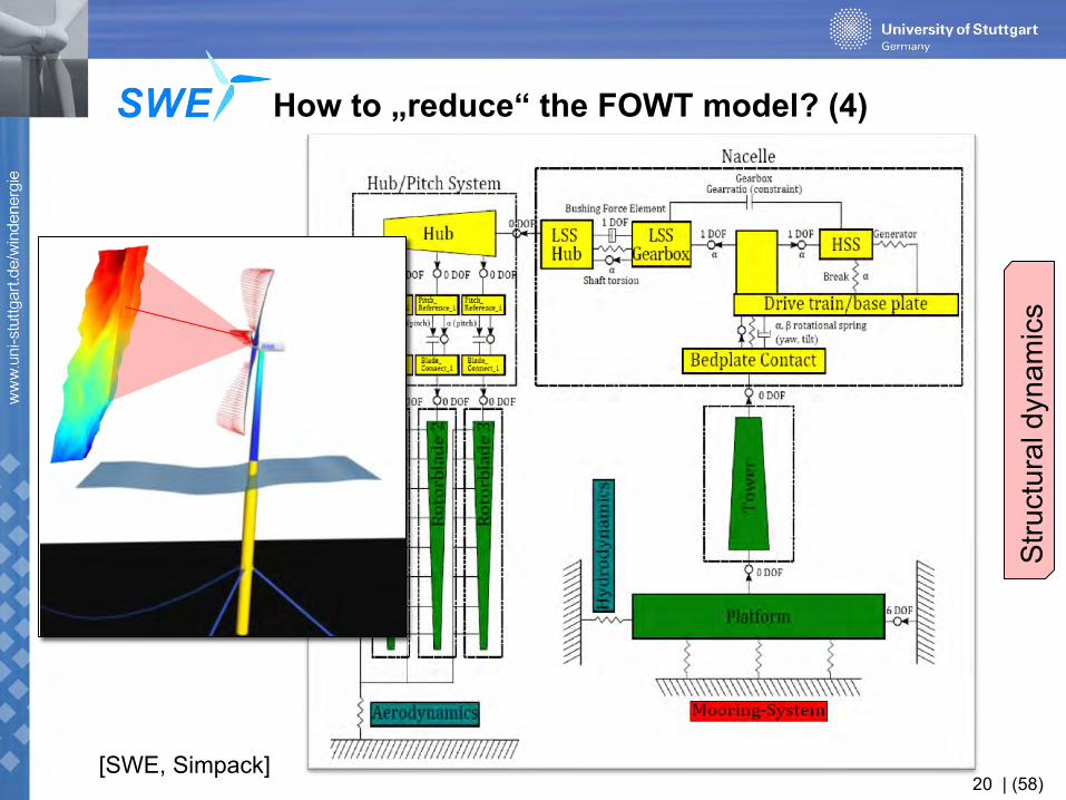
How to „reduce“ the FOWT model? (4)
• Gyroscopic effect? • Frequency range?
(selection of modes) • Extreme or fatigue
loads?
Stru
ctur
al d
ynam
ics
[SWE, Simpack]
22 | (58)
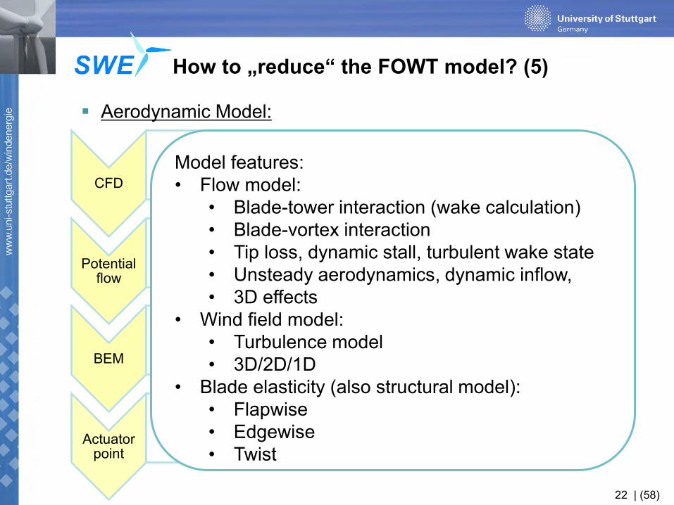
How to „reduce“ the FOWT model? (5)
Aerodynamic Model:
CFD
Potential flow
BEM
Actuator point
Model features: • Flow model:
• Blade-tower interaction (wake calculation) • Blade-vortex interaction • Tip loss, dynamic stall, turbulent wake state • Unsteady aerodynamics, dynamic inflow, • 3D effects
• Wind field model: • Turbulence model • 3D/2D/1D
• Blade elasticity (also structural model): • Flapwise • Edgewise • Twist
23 | (58)
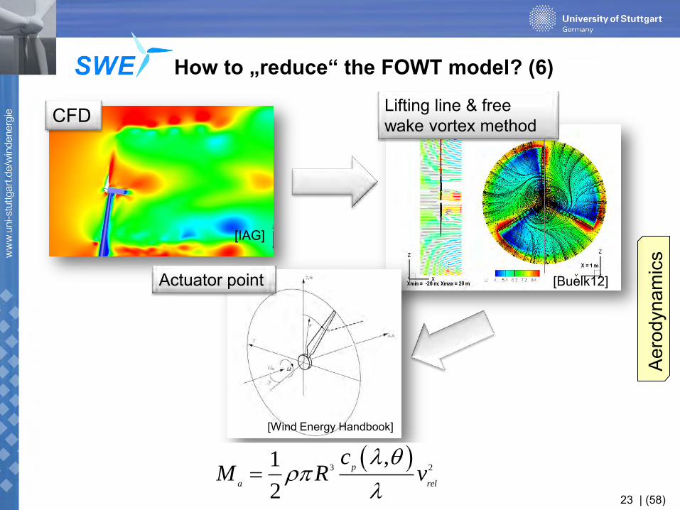
How to „reduce“ the FOWT model? (6)
[Buelk12]
[IAG]
[Wind Energy Handbook]
Aer
odyn
amic
s
3 2
,1
2
p
a rel
cM R v
CFD Lifting line & free wake vortex method
Actuator point
24 | (58)
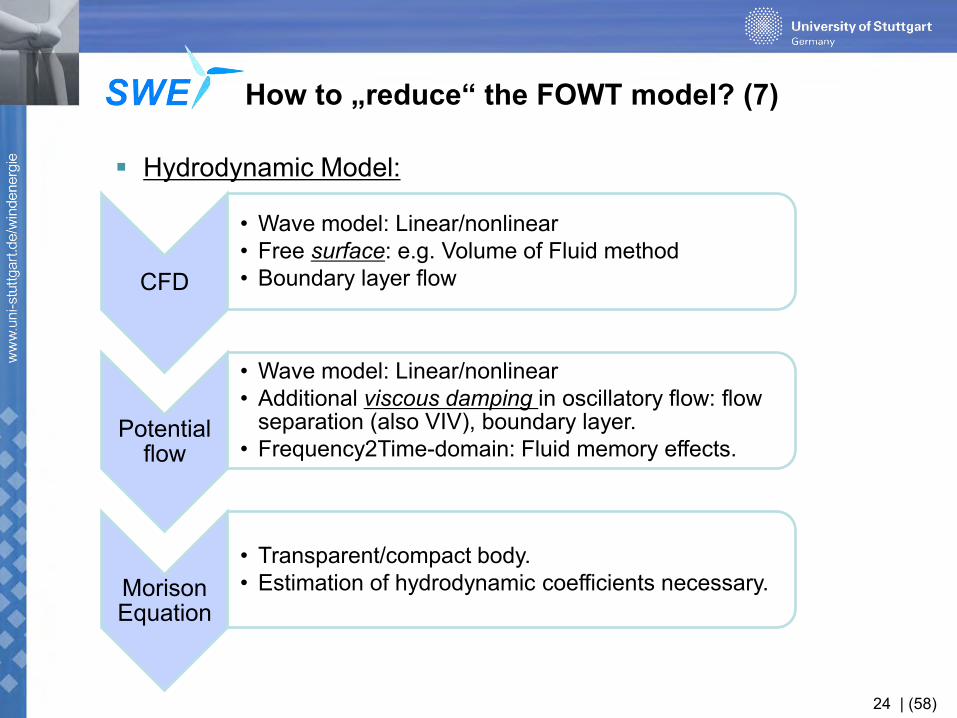
How to „reduce“ the FOWT model? (7)
Hydrodynamic Model:
CFD
• Wave model: Linear/nonlinear • Free surface: e.g. Volume of Fluid method • Boundary layer flow
Potential flow
• Wave model: Linear/nonlinear • Additional viscous damping in oscillatory flow: flow
separation (also VIV), boundary layer. • Frequency2Time-domain: Fluid memory effects.
Morison Equation
• Transparent/compact body. • Estimation of hydrodynamic coefficients necessary.
25 | (58)
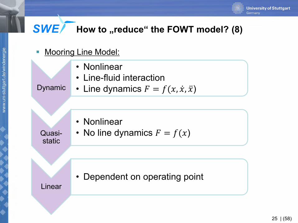
How to „reduce“ the FOWT model? (8)
Mooring Line Model:
Dynamic
• Nonlinear • Line-fluid interaction • Line dynamics 𝐹 = 𝑓(𝑥, 𝑥 , 𝑥 )
Quasi-static
• Nonlinear • No line dynamics 𝐹 = 𝑓(𝑥)
Linear • Dependent on operating point
26 | (58)
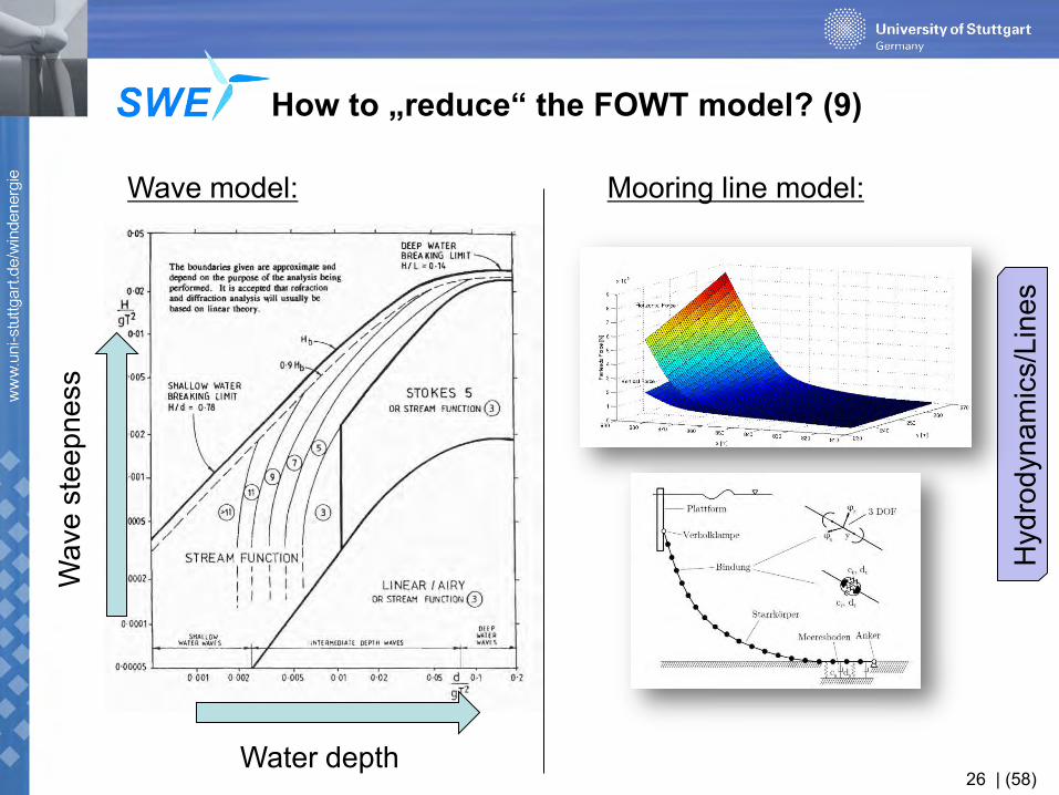
How to „reduce“ the FOWT model? (9)
Hyd
rody
nam
ics/
Line
s
Water depth
Wav
e st
eepn
ess
Mooring line model: Wave model:
27 | (58)
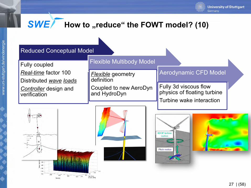
How to „reduce“ the FOWT model? (10)
Reduced Conceptual Model
Fully coupled Real-time factor 100 Distributed wave loads Controller design and verification
Flexible Multibody Model
Flexible geometry definition Coupled to new AeroDyn and HydroDyn
Aerodynamic CFD Model
Fully 3d viscous flow physics of floating turbine Turbine wake interaction
30 | (58)
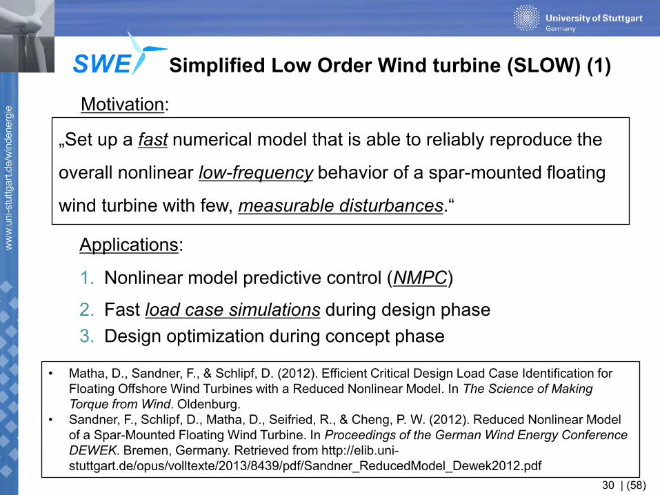
Simplified Low Order Wind turbine (SLOW) (1)
Applications:
1. Nonlinear model predictive control (NMPC)
2. Fast load case simulations during design phase 3. Design optimization during concept phase
„Set up a fast numerical model that is able to reliably reproduce the
overall nonlinear low-frequency behavior of a spar-mounted floating
wind turbine with few, measurable disturbances.“
• Matha, D., Sandner, F., & Schlipf, D. (2012). Efficient Critical Design Load Case Identification for Floating Offshore Wind Turbines with a Reduced Nonlinear Model. In The Science of Making Torque from Wind. Oldenburg.
• Sandner, F., Schlipf, D., Matha, D., Seifried, R., & Cheng, P. W. (2012). Reduced Nonlinear Model of a Spar-Mounted Floating Wind Turbine. In Proceedings of the German Wind Energy Conference DEWEK. Bremen, Germany. Retrieved from http://elib.uni-stuttgart.de/opus/volltexte/2013/8439/pdf/Sandner_ReducedModel_Dewek2012.pdf
Motivation:
31 | (58)
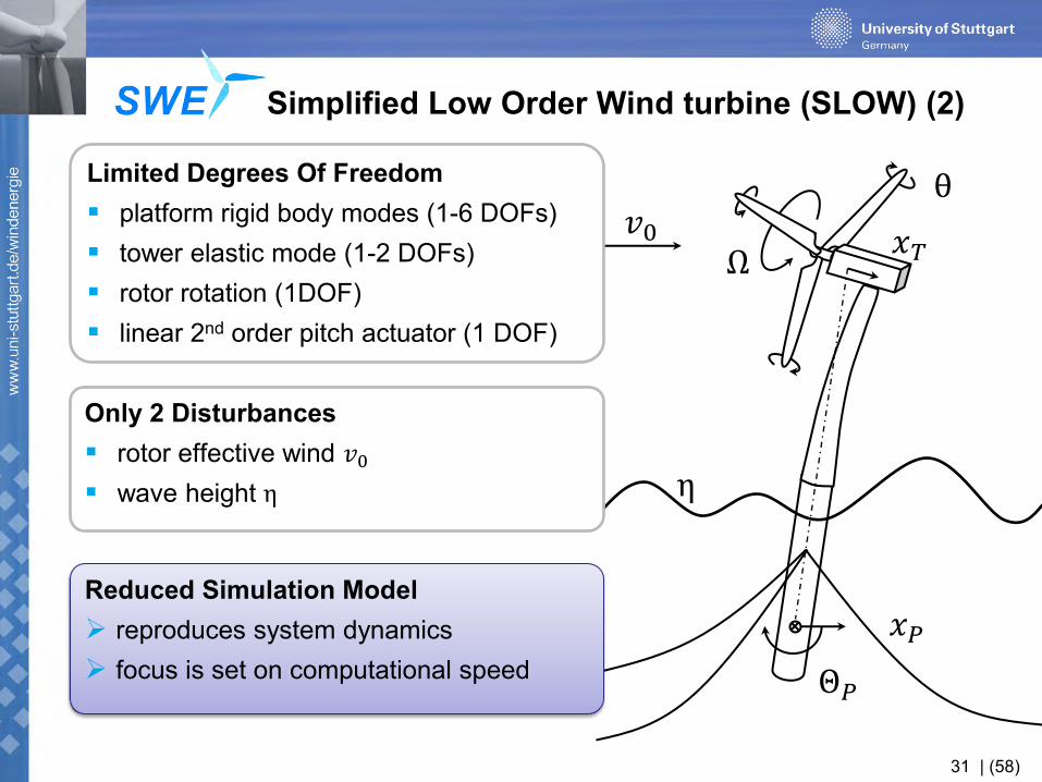
Simplified Low Order Wind turbine (SLOW) (2)
Ω
θ 𝑥𝑇 𝑣0
η
𝑥𝑃 Θ𝑃
Limited Degrees Of Freedom platform rigid body modes (1-6 DOFs) tower elastic mode (1-2 DOFs) rotor rotation (1DOF) linear 2nd order pitch actuator (1 DOF) Only 2 Disturbances rotor effective wind 𝑣0 wave height η
Reduced Simulation Model reproduces system dynamics focus is set on computational speed
32 | (58)
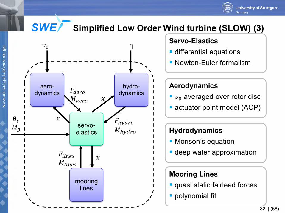
Simplified Low Order Wind turbine (SLOW) (3)
servo-elastics
θ𝑐𝑀𝑔
hydro-dynamics
η
𝑥
𝐹ℎ𝑦𝑑𝑟𝑜 𝑀ℎ𝑦𝑑𝑟𝑜
mooring lines
𝑥 𝐹𝑙𝑖𝑛𝑒𝑠 𝑀𝑙𝑖𝑛𝑒𝑠
aero-dynamics
𝑣0
𝑥
𝐹𝑎𝑒𝑟𝑜 𝑀𝑎𝑒𝑟𝑜
Servo-Elastics differential equations Newton-Euler formalism
Aerodynamics 𝑣0 averaged over rotor disc actuator point model (ACP)
Hydrodynamics Morison’s equation deep water approximation
Mooring Lines quasi static fairlead forces polynomial fit
34 | (58)
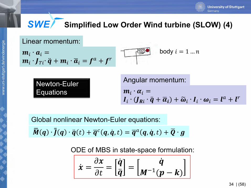
Simplified Low Order Wind turbine (SLOW) (4)
Newton-Euler Equations
𝒎𝑖 ∙ 𝒂𝑖 = 𝒎𝑖 ∙ 𝑱𝑇𝑖∙ 𝒒 + 𝒎𝑖 ∙ 𝒂 𝑖 = 𝒇𝑎 + 𝒇𝑟
Linear momentum:
Angular momentum:
𝑴 𝒒 ∙ 𝑱 𝒒 ∙ 𝒒 𝑡 + 𝒒 𝑐 𝒒, 𝒒 , 𝑡 = 𝒒 𝑎 𝒒, 𝒒 , 𝑡 + 𝑸 ∙ 𝒈
Global nonlinear Newton-Euler equations:
𝒙 =𝜕𝒙
𝜕𝑡=
𝒒 𝒒
=𝒒
𝑴−1(𝒑 − 𝒌)
ODE of MBS in state-space formulation:
body 𝑖 = 1…𝑛
𝒎𝑖 ∙ 𝜶𝑖 = 𝑰𝑖 ∙ (𝑱𝑹𝑖 ∙ 𝒒 + 𝜶 𝒊) + 𝝎 𝑖 ∙ 𝑰𝑖 ∙ 𝝎𝑖 = 𝒍𝑎 + 𝒍𝑟

35 | (58)
Simplified Low Order Wind turbine (SLOW) (5)
𝒗𝟎 = 𝟐𝟎𝒎
𝒔,𝑯𝒔 = 𝟔𝒎,𝑻𝒑 = 𝟏𝟎𝒔
36 | (58)
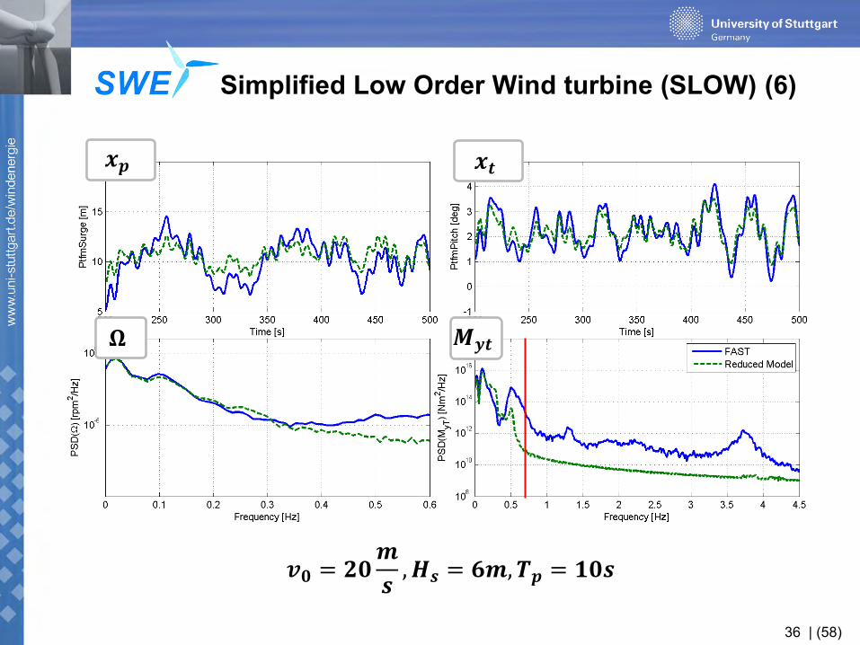
Simplified Low Order Wind turbine (SLOW) (6)
𝒗𝟎 = 𝟐𝟎𝒎
𝒔,𝑯𝒔 = 𝟔𝒎,𝑻𝒑 = 𝟏𝟎𝒔
𝒙𝒑 𝒙𝒕
𝛀 𝑴𝒚𝒕
37 | (58)
What‘s in this lecture?
• To get an understanding of the Floating Wind Turbine (FOWT) as a dynamic system and its modeling techniques.
• To get an idea of how to select the appropriate model simplification.
• To set up a first „coupled“ model.
39 | (58)
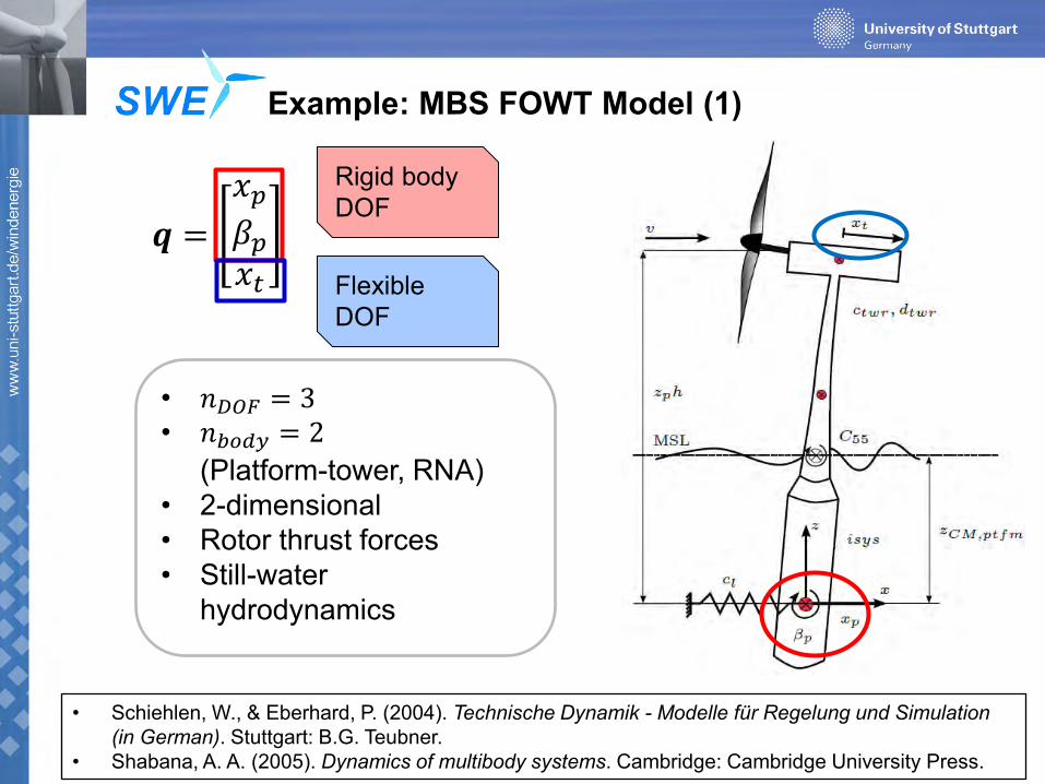
Example: MBS FOWT Model (1)
𝒒 =
𝑥𝑝𝛽𝑝𝑥𝑡
Rigid body DOF
Flexible DOF
• 𝑛𝐷𝑂𝐹 = 3 • 𝑛𝑏𝑜𝑑𝑦 = 2
(Platform-tower, RNA) • 2-dimensional • Rotor thrust forces • Still-water
hydrodynamics
• Schiehlen, W., & Eberhard, P. (2004). Technische Dynamik - Modelle für Regelung und Simulation (in German). Stuttgart: B.G. Teubner.
• Shabana, A. A. (2005). Dynamics of multibody systems. Cambridge: Cambridge University Press.
40 | (58)
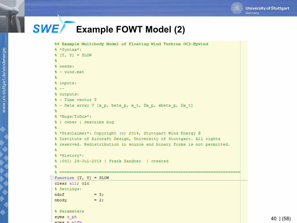
Example FOWT Model (2)

41 | (58)
Example: MBS FOWT Model (3)
𝒓𝑝𝑡𝑓𝑚 =
𝑥𝑝00
𝒓𝑛𝑎𝑐 = 𝑟𝑝𝑡𝑓𝑚 + 𝑺𝑝𝑡𝑓𝑚 ⋅
𝑥𝑡0𝑧𝑝ℎ
Position vectors platform, nacelle:
Rotation tensor:
𝑺 =
cos(𝛽𝑝) 0 sin(𝛽𝑝)
0 1 0−sin(𝛽𝑝) 0 cos(𝛽𝑝)
=
𝑥𝑝 + 𝑥tcos 𝛽𝑝 + 𝑧𝑝ℎsin(𝛽𝑝)
0−𝑥t sin 𝛽𝑝 + 𝑧𝑝ℎcos(𝛽𝑝)
= 𝑺𝑝𝑡𝑓𝑚 = 𝑺𝑟𝑛𝑎

42 | (58)
Example: MBS FOWT Model (4)
𝒎𝑖 ∙ 𝒂𝑖 = 𝒎𝑖 ∙ 𝑱𝑇𝑖∙ 𝒒 + 𝒎𝑖 ∙ 𝒂 𝑖 = 𝒇𝑎 + 𝒇𝑟
Linear momentum:
𝑱𝑡,𝑝𝑡𝑓𝑚 =1 0 00 0 00 0 0
𝒒 =
𝑥𝑝𝛽𝑝𝑥𝑡
𝑱𝑡,𝑖 =𝜕𝒓𝑖𝜕𝒒
Translational jacobian matrices:
𝒓𝑝𝑡𝑓𝑚 =
𝑥𝑝00
43 | (58)
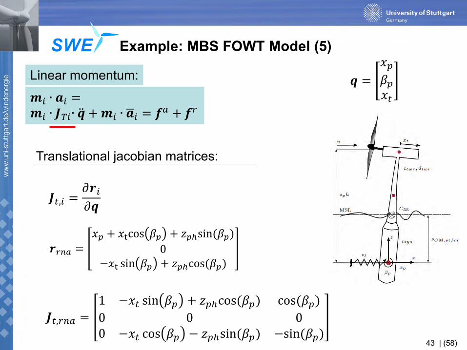
Example: MBS FOWT Model (5)
𝒎𝑖 ∙ 𝒂𝑖 = 𝒎𝑖 ∙ 𝑱𝑇𝑖∙ 𝒒 + 𝒎𝑖 ∙ 𝒂 𝑖 = 𝒇𝑎 + 𝒇𝑟
Linear momentum:
𝒓𝑟𝑛𝑎 =
𝑥𝑝 + 𝑥tcos 𝛽𝑝 + 𝑧𝑝ℎsin(𝛽𝑝)
0−𝑥t sin 𝛽𝑝 + 𝑧𝑝ℎcos(𝛽𝑝)
𝒒 =
𝑥𝑝𝛽𝑝𝑥𝑡
𝑱𝑡,𝑖 =𝜕𝒓𝑖𝜕𝒒
𝑱𝑡,𝑟𝑛𝑎 =
1 −𝑥𝑡 sin 𝛽𝑝 + 𝑧𝑝ℎcos(𝛽𝑝) cos(𝛽𝑝)
0 0 00 −𝑥𝑡 cos 𝛽𝑝 − 𝑧𝑝ℎsin(𝛽𝑝) −sin(𝛽𝑝)
Translational jacobian matrices:
44 | (58)
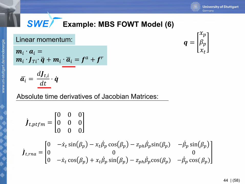
Example: MBS FOWT Model (6)
𝒎𝑖 ∙ 𝒂𝑖 = 𝒎𝑖 ∙ 𝑱𝑇𝑖∙ 𝒒 + 𝒎𝑖 ∙ 𝒂 𝑖 = 𝒇𝑎 + 𝒇𝑟
Linear momentum: 𝒒 =
𝑥𝑝𝛽𝑝𝑥𝑡
𝒂𝑖 = 𝑑𝑱𝑡,𝑖𝑑𝑡
⋅ 𝒒
𝑱 𝑡,𝑝𝑡𝑓𝑚 =0 0 00 0 00 0 0
𝑱 𝑡,𝑟𝑛𝑎 =
0 −𝑥 𝑡 sin 𝛽𝑝 − 𝑥𝑡𝛽 𝑝 cos 𝛽𝑝 − 𝑧𝑝ℎ𝛽 𝑝sin(𝛽𝑝) −𝛽 𝑝 sin 𝛽𝑝0 0 00 −𝑥 𝑡 cos 𝛽𝑝 + 𝑥𝑡𝛽 𝑝 sin 𝛽𝑝 − 𝑧𝑝ℎ𝛽 𝑝cos(𝛽𝑝) −𝛽 𝑝 cos( 𝛽𝑝)
Absolute time derivatives of Jacobian Matrices:
45 | (58)
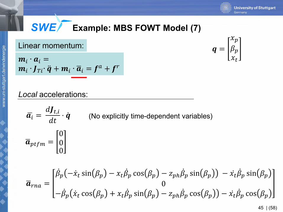
Example: MBS FOWT Model (7)
𝒎𝑖 ∙ 𝒂𝑖 = 𝒎𝑖 ∙ 𝑱𝑇𝑖∙ 𝒒 + 𝒎𝑖 ∙ 𝒂 𝑖 = 𝒇𝑎 + 𝒇𝑟
Linear momentum: 𝒒 =
𝑥𝑝𝛽𝑝𝑥𝑡
𝒂𝑖 = 𝑑𝑱𝑡,𝑖𝑑𝑡
⋅ 𝒒
Local accelerations:
𝒂 𝑝𝑡𝑓𝑚 =000
𝒂 𝑟𝑛𝑎 =
𝛽 𝑝 −𝑥 𝑡 sin 𝛽𝑝 − 𝑥𝑡𝛽 𝑝 cos 𝛽𝑝 − 𝑧𝑝ℎ𝛽 𝑝 sin 𝛽𝑝 − 𝑥𝑡 𝛽 𝑝 sin 𝛽𝑝0
−𝛽 𝑝 𝑥 𝑡 cos 𝛽𝑝 + 𝑥𝑡𝛽 𝑝 sin 𝛽𝑝 − 𝑧𝑝ℎ𝛽 𝑝 cos 𝛽𝑝 − 𝑥𝑡 𝛽 𝑝 cos 𝛽𝑝
(No explicitly time-dependent variables)

46 | (58)
Example: MBS FOWT Model (8)
𝑱𝑟,𝑝𝑡𝑓𝑚 = 𝑱𝑟,𝑛𝑎𝑐 =0 0 00 1 00 0 0
𝒒 =
𝑥𝑝𝛽𝑝𝑥𝑡
𝝎𝑖 = 𝑱𝑟𝑖 ⋅ 𝒒
𝑱 𝑟,𝑝𝑡𝑓𝑚 = 𝑱 𝑟,𝑛𝑎𝑐 =0 0 00 0 00 0 0
Angular momentum:
𝝎𝑝𝑡𝑓𝑚 = 𝝎𝑛𝑎𝑐 =0𝛽𝑝
0
Rotational jacobian matrices:
𝒎𝑖 ∙ 𝜶𝑖 = 𝑰𝑖 ∙ (𝑱𝑹𝑖 ∙ 𝒒 + 𝜶 𝒊) + 𝝎 𝑖 ∙ 𝑰𝑖 ∙ 𝝎𝑖 = 𝒍𝑎 + 𝒍𝑟
47 | (58)
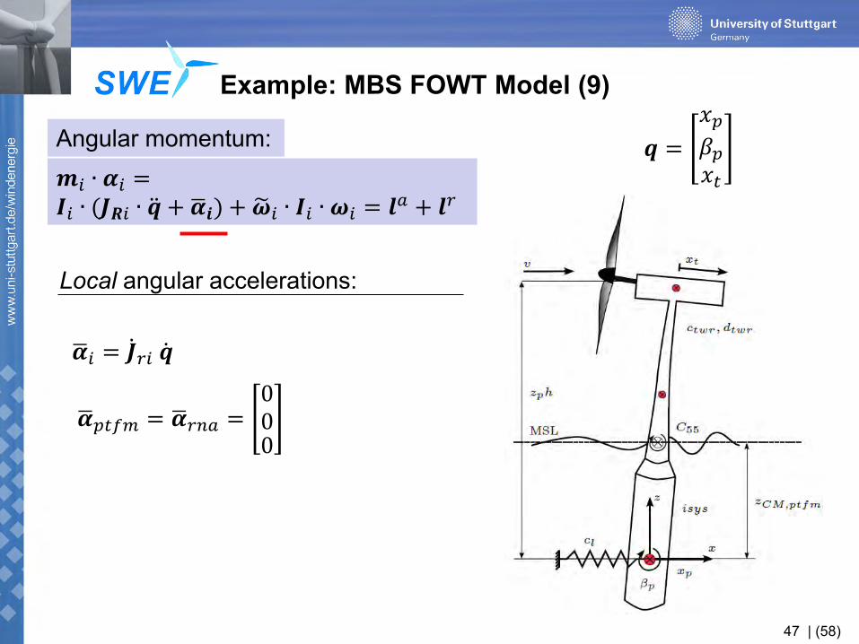
Example: MBS FOWT Model (9)
𝒒 =
𝑥𝑝𝛽𝑝𝑥𝑡
𝒎𝑖 ∙ 𝜶𝑖 = 𝑰𝑖 ∙ (𝑱𝑹𝑖 ∙ 𝒒 + 𝜶 𝒊) + 𝝎 𝑖 ∙ 𝑰𝑖 ∙ 𝝎𝑖 = 𝒍𝑎 + 𝒍𝑟
Angular momentum:
𝜶 𝑖 = 𝑱 𝑟𝑖 𝒒
Local angular accelerations:
𝜶 𝑝𝑡𝑓𝑚 = 𝜶 𝑟𝑛𝑎 =000

48 | (58)
Example: MBS FOWT Model (10)
𝒒 =
𝑥𝑝𝛽𝑝𝑥𝑡
𝒎𝑖 ∙ 𝜶𝑖 = 𝑰𝑖 ∙ (𝑱𝑹𝑖 ∙ 𝒒 + 𝜶 𝒊) + 𝝎 𝑖 ∙ 𝑰𝑖 ∙ 𝝎𝑖 = 𝒍𝑎 + 𝒍𝑟
Angular momentum:
Skew symmetric matrices:
𝝎 𝑝𝑡𝑓𝑚 = 𝝎 𝑛𝑎𝑐 =
00
0 𝛽 𝑝0 0
−𝛽 𝑝 0 0
𝑰𝑝𝑡𝑓𝑚 = 𝑺 ⋅ 𝑰′𝑝𝑡𝑓𝑚 ⋅ 𝑺𝑇
𝑰′𝑝𝑡𝑓𝑚 =
𝐼𝑥𝑥,𝑝 0 0
0 𝐼𝑦𝑦,𝑝 0
0 0 𝐼𝑧𝑧,𝑝
𝑰′𝑟𝑛𝑎 =
𝐼𝑥𝑥,𝑛 0 0
0 𝐼𝑦𝑦,𝑛 0
0 0 𝐼𝑧𝑧,𝑛
Cross-product operator:

49 | (58)
Example: MBS FOWT Model (11)
Thrust force in this model:
𝐹𝑤 =1
2𝜌𝜋𝑅2𝑐𝑇𝑣𝑟𝑒𝑙
2 𝑐𝑇: Steady-state values including NREL 5MW torque and blade-pitch controller
Thrust coefficient 𝑐𝑇 over wind speed 𝑣

50 | (58)
Example: MBS FOWT Model (12)
Hydrodynamic forces in this model:
• Hydrostatic restoring 𝐶55 • Linear damping 𝐵11, 𝐵55
51 | (58)
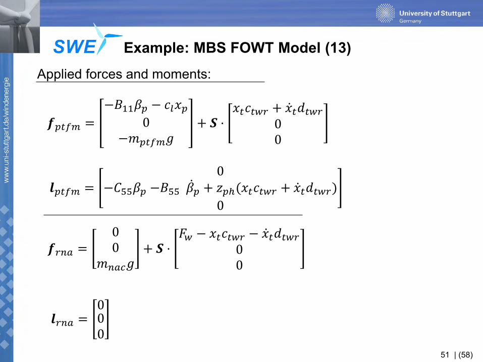
Example: MBS FOWT Model (13)
𝒇𝑝𝑡𝑓𝑚 =
−𝐵11𝛽𝑝 − 𝑐𝑙𝑥𝑝0
−𝑚𝑝𝑡𝑓𝑚𝑔+ 𝑺 ⋅
𝑥𝑡𝑐𝑡𝑤𝑟 + 𝑥 𝑡𝑑𝑡𝑤𝑟00
Applied forces and moments:
𝒍𝑝𝑡𝑓𝑚 =0
−𝐶55𝛽𝑝 −𝐵55 𝛽 𝑝 + 𝑧𝑝ℎ(𝑥𝑡𝑐𝑡𝑤𝑟 + 𝑥 𝑡𝑑𝑡𝑤𝑟)
0
𝒍𝑟𝑛𝑎 =000
𝒇𝑟𝑛𝑎 =00
𝑚𝑛𝑎𝑐𝑔+ 𝑺 ⋅
𝐹𝑤 − 𝑥𝑡𝑐𝑡𝑤𝑟 − 𝑥 𝑡𝑑𝑡𝑤𝑟00

52 | (58)
Example: MBS FOWT Model (14)
Global nonlinear Newton-Euler equations:
𝑴 𝒒 ∙ 𝑱 𝒒 ∙ 𝒒 𝑡 + 𝒒 𝑐 𝒒, 𝒒 = 𝒒 𝑎 𝒒, 𝒒 + 𝑸 ∙ 𝒈
𝑱 =
𝑱𝑡,𝑝𝑡𝑓𝑚𝑱𝑡,𝑟𝑛𝑎𝑱𝑟,𝑝𝑡𝑓𝑚𝑱𝑟,𝑟𝑛𝑎
𝑴 = 𝑴𝑝𝑡𝑓𝑚 𝑴𝑟𝑛𝑎𝑰𝑝𝑡𝑓𝑚𝑰𝑟𝑛𝑎
Global Jacobian matrix
Global mass matrix

53 | (58)
Example: MBS FOWT Model (15)
Global nonlinear Newton-Euler equations:
𝑴 𝒒 ∙ 𝑱 𝒒 ∙ 𝒒 𝑡 + 𝒒 𝑐 𝒒, 𝒒 = 𝒒 𝑎 𝒒, 𝒒 + 𝑸 ∙ 𝒈
𝒒 𝑐 =
𝑴𝑝𝑡𝑓𝑚 ⋅ 𝒂 𝑝𝑡𝑓𝑚𝑴𝑟𝑛𝑎 ⋅ 𝒂 𝑟𝑛𝑎
𝑰𝑝𝑡𝑓𝑚𝜶 𝒊 +𝝎 𝑝𝑡𝑓𝑚 ∙ 𝑰𝑝𝑡𝑓𝑚 ∙ 𝝎𝑝𝑡𝑓𝑚
𝑰𝑟𝑛𝑎𝜶 𝑟𝑛𝑎 +𝝎 𝑟𝑛𝑎 ∙ 𝑰𝑟𝑛𝑎 ∙ 𝝎𝑟𝑛𝑎
𝒒 𝑎 =
𝒇𝑝𝑡𝑓𝑚𝒇𝑟𝑛𝑎𝒍𝑝𝑡𝑓𝑚𝒍𝑟𝑛𝑎
Coriolis, centrifugal and gyroscopic forces and moments
Applied forces

54 | (58)
Example: MBS FOWT Model (16)
FOWT equations of motion:
𝑴 𝒒, 𝒒 ⋅ 𝒒 + 𝒌 𝒒, 𝒒 = 𝒑(𝒒, 𝒒 , 𝑡)
𝑱 𝑇 𝒒 ⋅ 𝑴 𝒒 ∙ 𝑱 𝒒 ∙ 𝒒 𝑡 + 𝑱 𝑇 𝒒 ⋅ 𝒒 𝑐 𝒒, 𝒒 = 𝑱 𝑇 𝒒 ⋅ 𝒒 𝑎 𝒒, 𝒒 + 𝑱 𝑇 𝒒 ⋅ 𝑸 ∙ 𝒈
Principle of d‘Alembert:
𝒙 =𝜕𝒙
𝜕𝑡=
𝒒 𝒒
=𝒒
𝑴−1(𝒑 − 𝒌)
State-space description:

55 | (58)
Example: MBS FOWT Model (17)
Model parameters:
𝑧𝑝ℎ 180 m 𝑚𝑝𝑡𝑓𝑚 7466330 kg
𝑚𝑟𝑛𝑎 350000 kg
𝐼𝑥𝑥,𝑝 = 𝐼𝑦𝑦,𝑝 4.7547x10⁹ kgm2
𝐼𝑥𝑥,𝑟 ≈ 𝐼𝑥𝑥,𝑟𝑜𝑡 4.0470x10⁷ kgm2
𝐼𝑦𝑦,𝑟 ≈ 𝐼𝑦𝑦,𝑟𝑜𝑡 = 𝐼𝑧𝑧,𝑟𝑜𝑡 =1
2𝐼𝑥𝑥,𝑟𝑜𝑡 2.0235x10⁷ kgm2
𝑐𝑡𝑤𝑟 2.2463045x10⁶ N/m
𝑑𝑡𝑤𝑟 5.65872x10³ Ns/m
𝑐𝑙 41180.0 N/m
𝐶55 2.2577x10⁹ Nm/rad
𝐵55 1x10⁶ Nms/rad
𝐵11 1x10⁶ Ns/m
𝑅 63 m
𝜌𝑎𝑖𝑟 1.225 kg/m3
𝑔 9.80665 N/kg

56 | (58)
Examplary MBS FOWT Model: Results (18)
𝒗𝟎
𝒙𝒑
𝜷𝒑
𝒙𝒕
57 | (58)
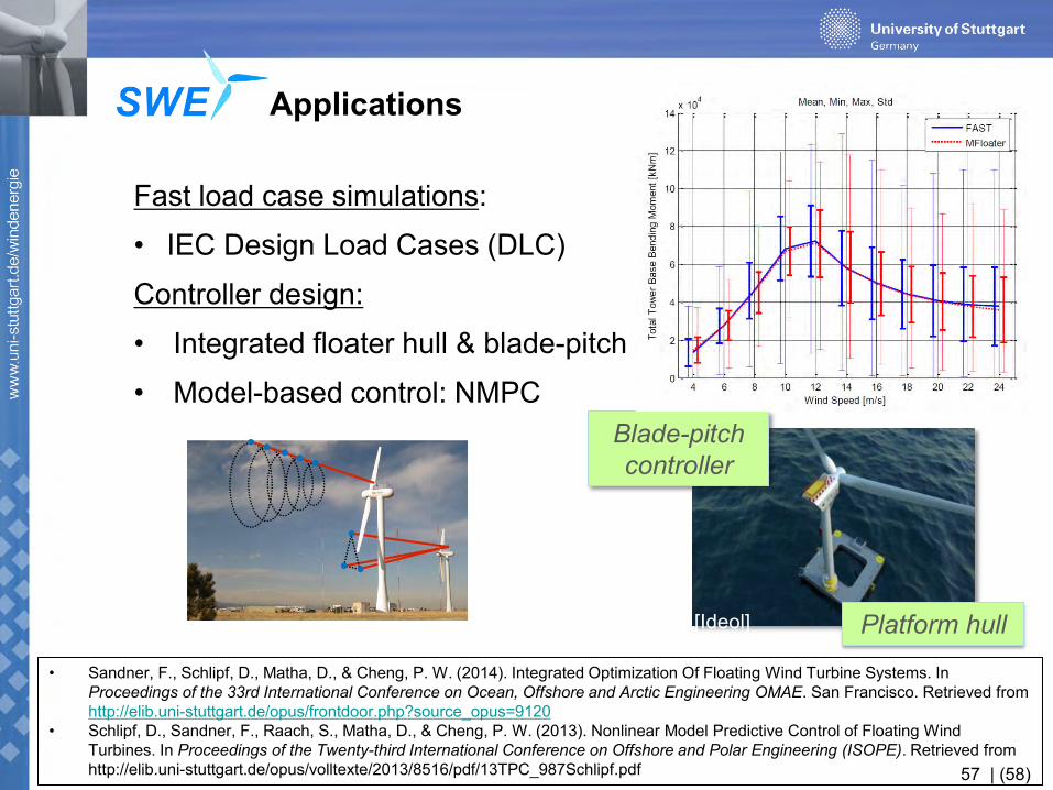
Applications
Fast load case simulations:
• IEC Design Load Cases (DLC)
Controller design:
• Integrated floater hull & blade-pitch controller design
• Model-based control: NMPC
Platform hull
Blade-pitch controller
[Ideol]
• Sandner, F., Schlipf, D., Matha, D., & Cheng, P. W. (2014). Integrated Optimization Of Floating Wind Turbine Systems. In Proceedings of the 33rd International Conference on Ocean, Offshore and Arctic Engineering OMAE. San Francisco. Retrieved from http://elib.uni-stuttgart.de/opus/frontdoor.php?source_opus=9120
• Schlipf, D., Sandner, F., Raach, S., Matha, D., & Cheng, P. W. (2013). Nonlinear Model Predictive Control of Floating Wind Turbines. In Proceedings of the Twenty-third International Conference on Offshore and Polar Engineering (ISOPE). Retrieved from http://elib.uni-stuttgart.de/opus/volltexte/2013/8516/pdf/13TPC_987Schlipf.pdf
58 | (58)
Conclusions & Takeaways
• A FOWT is a complex and multidisciplinary system: Appropriate modeling techniques have yet to be established.
• Simplified models help to understand the underlying dynamics.
• For each question there is one most appropriate mathematical model.
• A dynamic FOWT model should be coupled from the beginning of the design process.
• FOWT overall system dynamics can be modeled without complex software. The real-time factor of reduced SLOW model is about 100.
• A multibody system (MBS) is the central part of a FOWT model.
• A multi-DOF MBS can be fairly easily set up applying the Newton-Euler algorithm.
• Advantages of the reduced SLOW model: Standalone, computationally efficient, flexible modifications/add-ons.