reduced order surrogate modeling technique for …
TRANSCRIPT
REDUCED ORDER SURROGATE MODELING TECHNIQUE
FOR LINEAR DYNAMIC SYSTEMS
V. Yaghoubi, S. Rahrovani, H. Nahvi, S. Marelli
CHAIR OF RISK, SAFETY AND UNCERTAINTY QUANTIFICATION
STEFANO-FRANSCINI-PLATZ 5CH-8093 ZURICH
Risk, Safety &Uncertainty Quantification

Data Sheet
Journal: Mechanical Systems and Signal Processing
Report Ref.: RSUQ-2018-002
Arxiv Ref.: –
DOI: https://doi.org/10.1016/j.ymssp.2018.02.020
Date submitted: 7 May 2017
Date accepted: 10 February 2018
Reduced order surrogate modeling technique for linear dynamic
systems
Vahid Yaghoubi, Sadegh Rahrovani, Hassan Nahvi, Stefano Marelli
June 9, 2018
Abstract
The availability of reduced order models can greatly decrease the computational costs
needed for modeling, identification and design of real-world structural systems. However,
since these systems are usually employed with some uncertain parameters, the approximant
must provide a good accuracy for a range of stochastic parameters variations. The derivation
of such reduced order models are addressed in this paper. The proposed method consists of
a polynomial chaos expansion (PCE)-based state-space model together with a PCE-based
modal dominancy analysis to reduce the model order. To solve the issue of spatial aliasing
during mode tracking step, a new correlation metric is utilized. The performance of the
presented method is validated through four illustrative benchmarks: a simple mass-spring
system with four Degrees Of Freedom (DOF), a 2-DOF system exhibiting a mode veering
phenomenon, a 6-DOF system with large parameter space and a cantilever Timoshenko beam
resembling large-scale systems.
1 Introduction
Modeling and simulation (M&S) play important roles in the analysis, design, and optimiza-
tion of engineering systems. M&S targets deriving models with enough accuracy for their
intended purpose. These models can be used to predict the systems’ response under different
loading and environmental conditions. Although the development of computational power
of modern computers has been very fast in recent years, more precise description of model
properties and more detailed representation of the system geometry still result in large-scale,
more complex models of dynamical systems with considerable execution time and memory
usage. Model reduction Antoulas et al. (2001), efficient simulation Yaghoubi et al. (2016);
Avitabile and O’Callahan (2009); Liu et al. (2012) and parallel simulation methods Yaghoubi
et al. (2015); Tak and Park (2013) are different strategies to address this issue.
1
Nowadays, due to an ever increasing need for accurate and robust prediction of systems’
response, engineering models are almost always employed with some parameters to allow
variations in material properties, geometries, initial and boundary conditions. Consequently,
numerous model evaluations are normally required for the procedure of modeling, identifi-
cation and design of real-world applications in order to optimize the models’ performance.
This can be prohibitively expensive for computationally demanding models. In the literature,
several approaches address this issue by replacing such models with approximations that can
reproduce the essential features faster, e.g. surrogate modeling Frangos et al. (2010) and
parametric model order reduction (PMOR) Benner et al. (2013).
Surrogate models can be created intrusively or non-intrusively. In intrusive approaches,
the equations of a system are modified such that one explicit function relates the stochastic
properties of the system responses to the random inputs. The perturbation method Schueller
and Pradlwarter (2009) is a classical tool used for this purpose but it is only accurate when the
random inputs have small coefficients of variation (COV). An alternative method is intrusive
Polynomial Chaos Expansion (PCE) Ghanem and Spanos (2003). It was first introduced
for Gaussian input random variables Wiener (1938) and then extended to the other types of
random variables leading to generalized polynomial chaos Xiu and Karniadakis (2002); Soize
and Ghanem (2004). In non-intrusive approaches, already existing deterministic codes are
evaluated at several sample points selected over the parameter space. This selection depends
on the methods employed to build the surrogate model, namely regression Blatman and
Sudret (2010); Berveiller et al. (2006) or projection methods Gilli et al. (2013); Knio et al.
(2001). Kriging Fricker et al. (2011); Jones et al. (1998) and non-intrusive PCE Blatman and
Sudret (2011) or combination thereof Kersaudy et al. (2015); Schobi et al. (2015) are examples
of the non-intrusive approaches. The major drawback of PCE methods, both intrusive and
non-intrusive, is the large number of unknown coefficients in problems with large parameter
spaces, which is referred to as the curse of dimensionality Sudret (2007). Sparse Blatman and
Sudret (2008) and adaptive sparse Blatman and Sudret (2011) polynomial chaos expansions
have been developed to tackle this issue.
Parametric model order reduction (PMOR) methods are analogous to regression-based
non-intrusive surrogate modeling except that in PMOR, interpolations are performed not
only on system responses Baur et al. (2011), like surrogate modeling Yaghoubi et al. (2017),
but also on the reduced bases Amsallem and Farhat (2008) and reduced models Amsallem
and Farhat (2011); Panzer et al. (2010) evaluated over the parameter space. In this regard,
some attempts have been made recently to surrogate the models as well, e.g. the modal
models Manan and Cooper (2010); Dertimanis et al. (2017), NARX models Mai et al. (2016)
and time-varying ARMA models Bogoevska et al. (2017). However, they were only applied
to very small cases with single excitation and single sensor location, known as single-input,
single-output (SISO) systems. Since the extension of the modal models to nonlinear systems
2
is not straightforward and NARX models become very complex for structures with Multi-
input, Multi-output (MIMO), they are not a suitable model for real life applications.
State-space (SS) is the most common model for dynamic systems due to the following
reasons: (i) it can represent MIMO systems as convenient as SISO systems, (ii) it can easily
be expanded to the more complex physical phenomena such as nonlinear systems, time-
varying systems, etc. Unlike PMOR methods which are mostly developed for SS models
Benner et al. (2013), there is a lack of literature in surrogating these models. Moreover,
complex dynamic systems have large model orders, therefore applying PCE directly on these
models may not be feasible. An appropriate approach could be to construct surrogate models
jointly with a proper model reduction method which is at the focus of this paper. It opens
up a new field which requires more investigation.
In Yang et al. (2015), Yang et al. combine intrusive PCE with a projection based model
reduction method and applied them to uncertain structures. In Kim (2015), Kim developed a
reduced order modeling technique for parametric linear systems. In this method, Karhunen-
Loeve approach is used in frequency domain to calculate optimal modes subject to the
simultaneous excitations. The method has been successfully applied to a structural systems
and later in Kim (2016), was extended to aeroelastic systems.
The main contribution of this paper is developing a reduced-order PCE-based surrogate
model for linear dynamic systems when they are presented in SS form. For this purpose,
the PCE-based surrogate model is developed in conjunction with modal dominancy analysis
Rahrovani et al. (2014) in order to reduce the model order, if required, while preserving
the model structure. Computational efficiency is another beneficial feature of the modal
dominancy analysis which is of our special interest in this work. The proposed method is
organized around two steps. In the first step, the modes are transformed to have similar
orientations to those of a reference model and in the second step, interpolation is performed
using PCE. The other novelties of the paper are: (i) new correlation metric to track system
modes when small number of sensors are available, (ii): QR-factorization is employed to
treat the well-known problem of non-unique eigenvectors of coalescent modes.
The outline of the paper is as follows. In Section 2, the problem is formulated and in
Section 4, after a short review of the pertinent materials from linear system theories and
polynomial chaos expansion, the proposed methodology is elaborated. In Section 5, the
method is applied to several academic case studies resembling challenges in the structures.
2 Problem formulation
Consider the spatially-discretized governing second-order equation of motion of a linear time-
invariant (LTI) system as
3

M(x)q(t) + V (x)q(t) +K(x)q(t) = f(t)
y(t) = C ′(x)q(t)(1)
in which for an N -DOF system with nu system inputs and ny system outputs, q(t) ∈ RN
is the displacement vector, y(t) ∈ Rny is the system output, f(t) is the external load vector
which is governed by a transformation of stimuli vector f(t) = Puu(t); with u(t) ∈ Rnu . x ∈Rnx is the parameter vector and real positive-definite symmetric matrices M ,V ,K ∈ RN×N
are mass, damping and stiffness matrices, respectively. The output matrix C ′ ∈ Cny×N ,
maps the displacement vector to the output y(t).
The SS realization of the equation of motion in Eq. (1) can be written as
η(t) = A(x)η(t) +B(x)u(t)
y(t) = C(x)η(t) +D(x)u(t)(2)
where A ∈ C2N×2N , B ∈ C2N×nu , C ∈ Cny×2N , and D ∈ Cny×nu . η(t) = [q(t)T , qT (t)]T ∈R2N is the state vector. A and B are related to mass, damping and stiffness as follows
A =
0 I
−M−1V −M−1K
,B =
0
M−1P u
. (3)
The output matrix C maps the states to the output y and D is the associated direct
throughput matrix. Such system with order of 2N is denoted by
Σ(x) = A(x),B(x),C(x),D(x) ∈ O(2N).
In cases with large model orders, one can use model reduction methods to reduce the model
order to 2n 2N while retaining the main properties of the full model. For this purpose,
several methods have been proposed in the literature which have been comprehensively re-
viewed in Antoulas et al. (2001). One of these approaches is modal dominancy analysis
based on modal contributions Rahrovani et al. (2014) which is discussed more in Section
4.2. In this case, the reduced model Σr = Ar(x),Br(x),Cr(x),Dr(x) ∈ O(2n) can be
presented as
ηr(t) = Ar(x)ηr(t) +Br(x)u(t)
y(t) = Cr(x)ηr(t) +Dr(x)u(t)(4)
with ηr(t) ∈ R2n.
The problem is then as follows
Given Σ(k)NED
k=1 = Σ(x(k))NED
k=1 denoting systems evaluated at NED points sampled
from the parameter space x. The systems are assumed to be minimally realized linear time-
invariant(LTI) with equal number of states at all different realizations. Furthermore, let
x(0) 6= x(k), k = 1, 2, ..., NED be a new parameter set from the parameter space.
Find a method which can approximate Σr(x(0)) by making PCEs over the already
evaluated systems Σ(k)NED
k=1 .
4

3 Background
This section briefly reviews some features from linear system theories and polynomial chaos
expansions pertinent to the proposed method.
3.1 Linear system theories
In system theory, realization of an SS model is not unique. That is, given an input-output
relationship, a realization of an SS model is any quadruple of A,B,C,D1 such that
[u(t),y(t)] describes the input and output. Obviously, there are infinite number of realiza-
tions for an SS model which are called equivalent systems. They are defined as follows,
Definition 1. Let Σ ∈ O(2N) be a system in SS representation, T ∈ R2N×2N be a nonsin-
gular matrix and η = Tηe. Then, the model Σe = T (Σ) ∈ O(2N)
ηe(t) = Aeηe(t) +Beu(t)
ye(t) = Ceηe(t) +Deu(t)(5)
where
Ae = T−1AT ,Be = T−1B,Ce = CT ,De = D (6)
is said to be (algebraically) equivalent to Σ and T is called equivalence transformation.
A common SS realization is the modal realization which is discussed in the subsequent
section.
Modal realization
Assume that the dynamical system Σ ∈ O(2N) is diagonalizable and let A be a Hermitian
matrix with the eigenvalue set of λ = λ1, λ2, ..., λ2N and the corresponding eigenvector
matrix Φ = φ1,φ2, ...,φ2N. Using the transformation T = Φ the dynamical system Σ
can be projected onto modal coordinates in the form of the following quadruple,
Σ = Φ(Σ) = A, B, C,D = Φ−1AΦ,Φ−1B,CΦ,D (7)
where A = Λ = diag(λ1, λ2, ..., λ2N ), B = [b1, b2, ..., b2N ] is the modally projected input
matrix, and C=[c1, c2, ..., c2N ] is the modally projected output matrix. In particular, it
should be noted that the ith column of C is the projection of the ith eigenvector of A to the
space spanned by the output y.
3.2 Polynomial chaos expansion
Let M be a computational model with nx random inputs X=X1, X2, ..., XnxT and one
output Y . Assume that the random variables are independent and thus, their joint prob-
ability distribution function (PDF) defined in the probability space (Ω,F , P) is fX(x) =
1The dependency of the system matrices on parameters x has been dropped for simplicity
5
∏nx
i=1 fXi(xi). Further, the system response Y = M(X) is assumed to be a second-order
random variable, i.e. E[Y 2]< +∞ and belongs to the Hilbert space H = L 2
fX(Rnx ,R) of
fX -square integrable functions of X with respect to the inner product:
E [ψ(X)φ(X)] =
∫
DX
ψ(x)φ(x)fX(x)dx (8)
where DX is the support of X. In order to make polynomial chaos expansion for Y , let us
define multi-index set α = (α1, α2, ..., αnx) to which, any multivariate polynomials can be
constructed by
ψα(X) =
nx∏
i=1
ψ(i)αi
(Xi)
where ψ(i)αi (Xi), αi ∈ N is a univariate orthonormal polynomials defined with respect to
the marginal PDFs. For instance, if the inputs are standard normal or uniform variables,
the corresponding univariate polynomials are Hermite or Legendre polynomials, respectively.
The multivariate polynomials in the input vectorX are orthonormal with respect to the joint
PDF fX(x), i.e. :
E [ψα(X)ψβ(X)] =
∫
DX
ψα(x)ψβ(x)fX(x)dx = δαβ (9)
where δαβ is the Kronecker delta.
With these notations, the generalized polynomial chaos representation of Y reads Xiu
and Karniadakis (2002):
Y =∑
α∈Nnx
uαψα(X) (10)
in which uα is a set of unknown deterministic coefficients which can be estimated non-
intrusively by projection Ghanem and Ghiocel (1998); Ghiocel and Ghanem (2002) or least
square regression methods Blatman and Sudret (2010); Berveiller et al. (2006). The latter
is of interest here and will be briefly explained later on.
Prior to that, the infinite series in Eq.(10) has to be truncated. One approach is the
Standard truncation scheme which include all polynomials corresponding to the set Anx,p =
α ∈ Nnx : |α| ≤ p, where p is a maximum polynomial degree and |α| =∑nx
i=1 αi is the
total degree of polynomial ψα. The main drawback of this approach is rapid increase in the
cardinality of the set Anx,p =(nx+pp
)= P by increasing the number of parameters nx and
the order of polynomials p. However, in order to control it, suitable truncation strategies
such as q-norm hyperbolic truncation Blatman and Sudret (2010) have been developed that
drastically reduce the number of unknowns when nx is large.
In order to estimate uα by least square regression, the truncation error ε is minimized
via least square as follows:
Y =M(X) =∑
α∈Anx,p
uα ψα(X) + ε ≡ UTΨ(X) + ε (11)
6
To formulate this procedure, let X = x(1),x(2), ...,x(NED) be an experimental design with
NED space-filling samples of X and Y = y(1) = M(x(1)), y(2) = M(x(2)), ..., y(NED) =
M(x(NED)) be their associated system responses. Then, the minimization problem is
ˆU = arg minE[(U
TΨ(X)−M(X)
)2]. (12)
which admits a closed form solution as
ˆU = (ΨTΨ)−1ΨTY . (13)
Here Ψ is the matrix containing the evaluations of the Hilbertian bases, that is Ψij =
ψαj (x(i)), i = 1, 2, ..., NED, j = 1, 2, ..., P .
The accuracy of PCE will be improved by reducing the effect of over-fitting in least square
regression. This can be carried out by using sparse adaptive regression algorithms proposed
in Hastie et al. (2007); Efron et al. (2004). In particular, the Least Angle Regression (LAR)
algorithm has been demonstrated to be effective in the context of PCE by Blatman and
Sudret Blatman and Sudret (2011). Readers interested to know more about calculating the
PCE are referred to Marelli and Sudret (2015).
Vector-valued response
In the case of vector-valued response, i.e. Y ∈ RNY , NY > 1, one can apply the presented
approach componentwise. For models with large number of random outputs, this can make
the algorithm computationally intractable. To avoid that, one can extract the main sta-
tistical features of the vectorial random response by principal component analysis (PCA).
The concept has been adapted to the context of PCE by Blatman and Sudret Blatman and
Sudret (2013).
Let us perform sample-based PCA by rewriting the Y as the combination of its mean Yand covariance matrix as follows:
Y = Y +
NY∑
i=1
uivTi (14)
where the vi’s are the eigenvectors of the covariance matrix:
COV (Y) = E[(Y − Y)T(Y − Y)
]= [v1, ...,vNY
]
l1 . . . 0
. . .
0 . . . lNY
vT1...
vTNY
T
(15)
and the ui’s are vectors such that
ui = (Y − Y)vi. (16)
Then, Y can be approximated by the NY -term truncation:
7
Y = Y +
NY∑
i=1
uivTi , NY NY . (17)
Since Y and vTi are the mean and the eigenvectors of the system responses, respectively;
they are independent of the realization. Therefore, PC expansion can be applied directly on
the NY NY auxiliary variables ui. Besides, acknowledging the fact that the PCA is an
invertible transform, the original output can be retrieved directly from Eq. (17) for every
new prediction of u.
4 Methodology
This section elaborate the proposed methodology to develop the reduced order PCE-based
surrogate model for linear dynamic system. It consists of three major steps: (i) Tracking the
eigensolution of a system while its parameters are varying, (ii) Ranking the modes based on
their contribution to the input/output relation (iii) Making PCE-based surrogate model.
4.1 Correlation-based mode tracking
Mode tracking is an approach applicable to eigenvalue problems with variable parameters in
order to maintain correspondence between reference and perturbed eigensolutions. For this
purpose, one of the approaches is correlation-based methods, e.g. the method based on Modal
Assurance Criteria (MAC) Kim and Kim (2000). However, the MAC shows shortcomings
in some situations. In the next section, these problems are elaborated and an alternative
method to solve the issues is proposed.
4.1.1 Dealing with spatial aliasing
Historically, the MAC was developed to measure the consistency between different estimates
of a modal vector Allemang (2003). It works properly for systems with well-separated reso-
nance frequencies and with many response locations for the representation of modal vectors.
However, when few sensors are available to estimate the experimental modal vectors, high
MAC correlations may occur between modal vectors of the modes associated with different
resonance frequencies. This is the spatial aliasing phenomenon which is related to observabil-
ity of the system. Observability indicates the ability of the system to determine the internal
states by the knowledge of the selected system outputs. An LTI system, with A ∈ C2N×2N
is said to be observable if its observability matrix O(A,C) has full rank, i.e.
rank(O(A,C)) = rank
C
CA...
CA2N−1
= 2N (18)
8

The relationship between the system’s observability and modal properties is thus of spe-
cial interest and motivated the development of the Modal Observability Correlation (MOC)
metric, first proposed in Yaghoubi and Abrahamsson (2014). To this end, let O(A, C) be
the observability matrix of a linear system presented in the modal form,
O(A, C) =
CΦ
CΦΛ...
CΦΛ2N−1
=
Cφ1 Cφ2 . . . Cφ2N
Cφ1λ1 Cφ2λ2 . . . Cφ2Nλ2N
......
. . ....
Cφ1λ2N−11 Cφ2λ
2N−12 . . . Cφ2Nλ
2N−12N
(19)
then, the modal observability vectors, oi, i = 1, 2, . . . , 2N , are defined as the columns of the
modal observability matrix, i.e.
O(x) = O(A(x), C(x)) =[o1(x) o2(x) . . . o2N (x)
](20)
Each modal observability vector has the following important properties: (i) it contains infor-
mation related to only one single vibrational mode, (ii) it includes the information of both
eigenvector and eigenvalue, (iii) it relates the modal parameters to the observability of the
modes given by a used sensor configuration. These properties suggest replacing eigenvectors
in MAC by the modal observability vectors. Hence, for the correlation between two modal
observability matrices O(xi) and O(xj), we have
MOC(O(xi),O(xj)) =|O(xi)
∗O(xj)|2|O(xi)∗O(xi)||O(xj)∗O(xj)|
, (21)
We call this metric the Modal Observability Correlation (MOC)2. Due to the property (ii)
of the vectors oi, i = 1, 2, . . . , 2N , this metric discriminates between two highly correlated
modal vectors with non-coinciding eigenvalues. This thus, makes MOC more powerful than
MAC in dealing with the problem of spatial aliasing. It should be mentioned that raising
the exponent of Λ, see Eq.(19), may cause numerical problems. In order to avoid that, the
MOC is evaluated for the eigenvalues of the discrete-time system which are located in the
complex plane unit disc. This means, the eigenvalues of the continuous-time systems, λj , j =
1, 2, . . . , 2N are transformed to the discrete-time counterpart using λdiscj = exp(λjτ) with an
arbitrary time step τ . Here, τ = π/fmax in which fmax is the maximum eigenfrequency of
the system. This leads to a distribution of the discrete-time eigenvalues λdiscj over a large
domain of the unit disc and thus separates them well.
4.1.2 Dealing with coalescent eigenvalues
Due to the nonunique eigenvectors of coalescent or closely spaced eigenvalues, their presence
in one system become one of the major challenges in both mode tracking and modal domi-
2This is called bMOC in Yaghoubi and Abrahamsson (2014)
9
nancy analysis. Therefore, it should be handled before any correlation analysis or dominancy
analysis takes place.
For this purpose, let Φj ∈ C2N×nc represent a matrix containing the linear independent
eigenvectors associated with a coalescent eigenvalue λj of multiplicity nc3. Moreover, let V be
the nc-dimensional space spanned by the columns of Φj . Since this is an A-invariant subspace
of C2N , any vector that lies there can be considered as an eigenvector corresponding to λj .
Therefore, different variants of a linearly independent basis for V may appear in repeated
system realizations. To treat this issue, a fixed orthogonal basis for V is established by
applying the QR-decomposition method on the projection of the columns of the system
input matrix B onto V , i.e. PV (B). That is,
PV (B) = Φj(Φ∗jΦj)
−1Φ∗jB (22)
where PV (B) ∈ C2N×nu . The QR-decomposition of PV (B) gives
PV (B) = QR (23)
here, Q ∈ C2N×2N is an orthogonal matrix and R ∈ R2N×nu is an upper triangular matrix.
The fixed orthogonal basis for V can then be constructed by the first nc columns of Q, i.e. ,
V = Span(q1, q2, . . . , qnc) (24)
The space spanned by the columns qi is also A-invariant and thus the unique vectors
qi, i = 1, 2, . . . , nc are eigenvectors associated with the coalescent eigenvalues, λj Laub (2005).
By that, the problem of nonunique eigenvector of coalescent eigenvalues is circumvented. This
decomposition will be employed throughout this study to fix the eigenvectors of coalescent
modes which may appear in the realization stage.
4.2 Modal dominancy analysis based on modal contribution into
system input/output relation
Given an SS model of a dynamical system Σ, by performing Laplace transformation, its
transfer function can be obtained as
G(s) = C(sI2N −A)−1B +D, s ∈ C (25)
Assume Σ = Φ(Σ) as presented in Eq. (7) is its associated minimal modal realization, and
let
G(−i)(s) =cibis− λi
(26)
3Due to the controllability reasons, the dimension nc cannot exceed the number of actuators, nu.
10

be the transfer function of the error system resulting from deflation of the ith modal co-
ordinate from Σ. Then, the contribution of the ith modal coordinate to the input-output
relation of the system in the H2 sense can be defined as Rahrovani et al. (2014),
MCH2= ‖G(−i)(jω)‖H2
=1
πtrb∗i c∗i cibi[
1
Re(λi)arctan(
ω
Re(λi))]∞−|Im(λi)| (27)
Here (•)∗ stands for Hermitian operation, Re and Im respectively, denote real and imaginary
parts of a complex number. H2 norm indicates the average error over frequency range of
interest induced by removing the ith modal coordinate Antoulas (2005). In general, it can
be assumed that the more important a mode is, the larger will be its contribution to the
input-output relation. Therefore, this measure can be a useful indication of dominancy for
the modes. By using it, a system can be partitioned into two subsystems: a dominant and
a weak one. The dominant one can be thus chosen as the reduced model. Let the system Σ
in Eq. (7) be partitioned as,
˙η1(t)
˙η2(t)
=
A11 A12
A21 A22
η1(t)
η2(t)
+
B1
B2
u(t)
y(t) =[C1 C2
]η1(t)
η2(t)
+ Du(t)
(28)
then, a reduced-order model can be obtained by truncating η2,
˙η1(t) = A11η1(t) + B1u(t)
y(t) = C1η1(t) + Du(t)(29)
or residualizing η2, i.e. ˙η2 = 0,
˙η1(t) = A11η1(t) + B1u(t)
y(t) = C1η1(t) + (C2A−122 B2 + D)u(t)
(30)
Readers interested in detailed discussions about this method are referred to Antoulas (2005).
4.3 PCE-based reduced order model
As mentioned in Def. 1, one system can have numerous equivalent systems, therefore after re-
alizations and before interpolation, one should transform the systems such that they all have
the same orientation. Therefore, the proposed method is presented as a two-step method.
Step I is to perform isometric transformations and step II is to calculate the corresponding
polynomial chaos expansion.
4.3.1 Step I: Isometric transformation
In this section, a proper isometric transformation is presented. In order to keep the diagonal
form of the models, transformations are applied to each individual state separately. For
11

this purpose, first, one system is chosen as the reference model Σref
and the others are
transformed such that their modes have the same order and orientation as the reference
ones. These transformations, illustrated in Fig. 1 for a 2-DOF system, are:
1. Permutation transformation P: This transformation is devised to track the modes and
treat the mode crossing phenomenon which is frequently occurred when parameters
are varying in a system. For this purpose, each system is compared to the reference
by using MOC and then its associated observability columns are permuted to obtain a
diagonal MOC matrix, i.e. for j = 1, 2, .., NED
P(Σ(j)
) = P(j)|diag(MOC(O(j),Oref )P(j)) = diag(√1,√2, . . . ,√2N ), (31)
in which
√i = max(MOC(o(j)i ,Oref )), i = 1, 2, . . . , 2N (32)
The transformed system is thus,
Σ(j)
= P(Σ(j)
) = PA, B, C,D = A, B, C,D (33)
Fig. 1a and Fig. 1b, respectively, illustrate eigenvectors of a 2-DOF system as are
realized and after applying the permutation P. The influence of this transformation
can be simply observed.
2. Rotation transformation R: This transformation could be obtained by minimizing the
distance between the ci and crefi in a suitable norm. This can translate as the following
minimization problem,
min∇i∈C
‖ci∇i − crefi ‖2F , i = 1, 2, . . . , 2N (34)
in which ‖•‖F stands for the Frobenius norm. The solution to this minimization prob-
lem is simply the projection of ci into the direction of crefi , i.e. for i = 1, 2, . . . , 2N
∇i =cTi c
refi
‖cTi crefi ‖, (35)
and therefore, the associated state is transformed as
λi, bi, ci = ∇i(λi, bi, ci) = ∇−1i λi∇i,∇−1i bi, ci∇i, (36)
and the rotated system can be thus written as
Σ(j)
= R(Σ(j)
) = RA, B, C,D = A, B, C,D, j = 1, 2, .., NED (37)
here R = diag(∇1,∇2, . . . ,∇2N ), A = diag(λ1, λ2, . . . , λ2N ), B = [b1, b2, . . . , b2N ] and
C = [c1, c2, . . . , c2N ]. Fig. 1c shows the effect of the transformation R on the direction
of the eigenvectors.
12
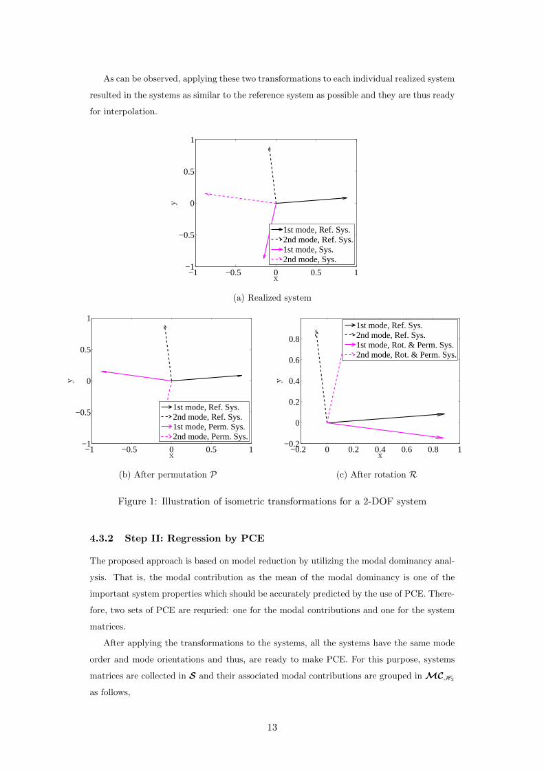
As can be observed, applying these two transformations to each individual realized system
resulted in the systems as similar to the reference system as possible and they are thus ready
for interpolation.
−1 −0.5 0 0.5 1−1
−0.5
0
0.5
1
x
y
1st mode, Ref. Sys.2nd mode, Ref. Sys.1st mode, Sys.2nd mode, Sys.
(a) Realized system
−1 −0.5 0 0.5 1−1
−0.5
0
0.5
1
x
y
1st mode, Ref. Sys.2nd mode, Ref. Sys.1st mode, Perm. Sys.2nd mode, Perm. Sys.
(b) After permutation P
−0.2 0 0.2 0.4 0.6 0.8 1−0.2
0
0.2
0.4
0.6
0.8
x
y
1st mode, Ref. Sys.2nd mode, Ref. Sys.1st mode, Rot. & Perm. Sys.2nd mode, Rot. & Perm. Sys.
(c) After rotation R
Figure 1: Illustration of isometric transformations for a 2-DOF system
4.3.2 Step II: Regression by PCE
The proposed approach is based on model reduction by utilizing the modal dominancy anal-
ysis. That is, the modal contribution as the mean of the modal dominancy is one of the
important system properties which should be accurately predicted by the use of PCE. There-
fore, two sets of PCE are requried: one for the modal contributions and one for the system
matrices.
After applying the transformations to the systems, all the systems have the same mode
order and mode orientations and thus, are ready to make PCE. For this purpose, systems
matrices are collected in S and their associated modal contributions are grouped in MCH2
as follows,
13
S = Σ(1), Σ
(2), . . . , Σ
(NED) =
diag(A(1)
), vect(B(1)
), vect(C(1)
), vect(D(1)))diag(A
(2)), vect(B
(2)), vect(C
(2)), vect(D(2))
...
diag(A(NED)
), vect(B(NED)
), vect(C(NED)
), vect(D(NED))
(38)
MCH2 = [MC1,H2 ,MC2,H2 , . . . ,MCN,H2 ] (39)
in which diag(·) stands for diagonal elements of the matrix (·), vect(·) denotes vectorizing
operation,
MCi,H2= [MC
(1)i,H2
,MC(2)i,H2
, . . . ,MC(NED)i,H2
]T i = 1, 2, . . . , N,
here (·)T denotes transpose operation.
In order to make PCE, since system’s matrices are normally complex-valued whereas,
the PCE which is selected as the regression method here, is only defined for real-valued
functions4, separate PCEs need to be performed for real and imaginary parts of the S. Note
that, PCE could also be made for amplitude and phase of the S however, based on the
authors’ experience, expansions on real and imaginary parts are more robust. Therefore, the
matrices SRe = real(S) and SIm = imag(S) are the matrices for which the PCE should
be made. Besides that, a system’s matrices normally occur in complex conjugate pairs. It
means that PCE can be made only for one of each pair and the other will be constructed
afterward, i.e. S ∈ CNED×(N(1+nu+ny)+nu×ny).
The number of random outputs for this set, NY = 2×NED× (N(1+nu+ny)+nu×ny),
can be extremely large. As discussed in Section 3.2, the PCEs are therefore applied directly
to the principal components of S, yielding:
SRe= E
[SRe
]+
NY∑
j=1
∑
α∈AM,p
(uReα ψα(x))jv
ReT
j , (40)
SIm= E
[SIm
]+
NY∑
j=1
∑
α∈AM,p
(uImα ψα(x))jvImT
j , (41)
where uReα and uImα are respectively the vectors of coefficients of the PCEs made for the real
and imaginary parts of the S.
The next set of PCE will be made for the modal contributions collected in the matrix
MCH2. Since the number of random outputs for this set is not very large, PCE can be
applied directly to them i.e. for i = 1, 2, · · · , N
MCi,H2=
∑
α∈AM,p
mcH2α (i)ψα(x). (42)
4Limited literature is available on the use of PCE for complex-valued functions, see e.g. Soize and Ghanem
(2004).
14

where mcH2 is the vector of coefficients of the PCEs. The proposed approach is formulated
in Algorithm 1.
4.3.3 PCE-based model reduction and response prediction
In order to obtain a reduced model at new sample point x(0), one can evaluate the whole
PCE-based SS model to make a full-order system and then reduce it using any truncation
scheme, or alternatively, select the dominant modes and evaluate PCEs only at those modes
to make a reduced-order SS model. Latter has been selected in this paper due to its efficiency
in time and memory usage.
For this purpose, two steps should be taken: (i) PCE-based model reduction, and (ii)
PCE-based model prediction. For the first step, one should evaluate Eq. (42) to obtain
contribution of the modes MCi,H2i = 1, 2, · · · , N and then, sort them in right order to
determine the first n modes to construct the dominant subsystem, see Eq. (28).
As the second step, Eqs. (40) and (41) are evaluated for the n selected modes to obtain
SRe
r (x(0)) and SIm
r (x(0)), respectively. Then the matrix Sr(x(0)) ∈ C1×(n(1+nu+ny)+nu×ny)
can be constructed by SRe
r (x(0)) + jSIm
r (x(0)), j =√−1 and in turn, the system matrices
can be constructed by an inverse vectorization operation. The algorithm for predicting the
response of the reduced model at a new sample point is briefly presented in Algorithm 2.
15

Algorithm 1 Proposed PCE-based surrogate modeling for SS models
1: Input: X = x(1),x(2), ...,x(NED)Step I: Isometric transformations
2: Σref
=Σ(x(r))=A(x(r)), B(x(r)), C(x(r)),D(x(r)), for a random r ∈ [1, ..., NED]
3: for k = 1 to NED do
4: Σk=Σ(x(k))=A(x(k)), B(x(k)), C(x(k)),D(x(k)) using Eq. (7)
5: Compute permutation transformation P using Eq.(31)
6: Evaluate Σk
= P(Σk) = PA, B, C,D = A, B, C,D
7: for i = 1 to N do
8: Compute ∇i =cTi c
refi
‖cTi crefi ‖9: end for
10: R = diag(∇1,∇2, . . . ,∇N )
11: Evaluate Σ(k)
= R(Σ(k)
) = RA, B, C,D = A, B, C,D12: Evaluate MC
(k)H2
= [MC(k)1,H2
,MC(k)2,H2
, . . . ,MC(k)N,H2
] using Eq. (27)
13: end for
Step II: Interpolation by PCE
14: S = Σ(1), Σ
(2), . . . , Σ
(NED) ∈ CNED×(N(1+nu+ny)+nu×ny),
SRe=real(S), SIm=imag(S)
15: MCi,H2 = [MC(1)i,H2
,MC(2)i,H2
, . . . ,MC(NED)i,H2
]T i = 1, 2, . . . , N,
16: Polynomial chaos expansion,
SRe: PCE of SRe using Eq. (40)
SIm: PCE of SIm using Eq. (41)
MCi,H2 : PCE of MCi,H2 using Eq. (42), i = 1, 2, . . . , N
17: MCH2 = [MC1,H2 ,MC2,H2 , . . . ,MCN,H2 ]
18: Output: SRe, SIm
, MCH2
16

Algorithm 2 Predicting reduced system’s responses
1: Input: x(0) 6= x(l), l = 1, 2, ..., NED
Step I: Model reduction:
2: for i = 1 to N do
3: Evaluate MCi,H2(x(0)) using Eq. (42)
4: end for
5: MCH2 = [MC1,H2 ,MC2,H2 , . . . ,MCN,H2 ]
6: Sort MCH2 in right order and select first n dominant modes
Step II: Model construction:
7: Evaluate SRer = SRe
(x(0)) using Eq. (40) for the n selected modes.
8: Evaluate SImr = SIm
(x(0)) using Eq. (41) for the n selected modes.
9: Sr=SRer + jSIm
r ∈ C1×(n(1+nu+ny)+nu×ny), j =√−1
10: Construct ˆΣ(0)r from Sr by inverse vectorization and diagonalization operations
11: Output: ˆΣ(0)r = ˆΣr(x
(0))
5 Case studies
5.1 Introduction
In this section, the proposed method will be applied to four case studies, (i) a simple 4-DOF
system to illustrate how the method works, (ii) a 2-DOF system representing the complex
phenomenon of mode veering, (iii) a 6-DOF system with a relatively large (16-dimensional)
parameter space. (iv) a 3D Timoshenko cantilever beam representing a large-scale model.
For the sake of readability, for the last two cases with 6 outputs, only results for one of the
outputs are shown.
To assess the accuracy of the proposed PCE-based model reduction approach quantita-
tively, the following measure based on the root mean square (rms) error of the vectors is
defined.
Error(·) =rms((·)ex − (·)approx))
rms((·)ex)× 100%, (43)
in which (·) is a vector of interest which could be the frequency response of a system in a
specific frequency band. (·)ex and (·)approx represent results obtained by the exact and the
approximate model, respectively. The definition of exact and approximate model will be
mentioned in the context.
17
Before analyzing the examples, following models should be described: (i) Full model: the
true model with the order of 2N , (ii) Direct reduced order model (ROM): the true model
reduced to order of 2n by the method of dominancy analysis (iii) PCE-based ROM: the
PCE-based model with the order of 2n. It should be emphasized that, in all examples, the
dominancy analysis has been carried out with state residualization technique, Eq. (30).
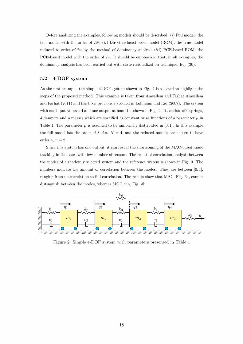
5.2 4-DOF system
As the first example, the simple 4-DOF system shown in Fig. 2 is selected to highlight the
steps of the proposed method. This example is taken from Amsallem and Farhat Amsallem
and Farhat (2011) and has been previously studied in Lohmann and Eid (2007). The system
with one input at mass 4 and one output at mass 1 is shown in Fig. 2. It consists of 6 springs,
4 dampers and 4 masses which are specified as constant or as functions of a parameter µ in
Table 1. The parameter µ is assumed to be uniformely distributed in [0, 1]. In this example
the full model has the order of 8, i.e. N = 4, and the reduced models are chosen to have
order 4, n = 2.
Since this system has one output, it can reveal the shortcoming of the MAC-based mode
tracking in the cases with few number of sensors. The result of correlation analysis between
the modes of a randomly selected system and the reference system is shown in Fig. 3. The
numbers indicate the amount of correlation between the modes. They are between [0, 1],
ranging from no correlation to full correlation. The results show that MAC, Fig. 3a, cannot
distinguish between the modes, whereas MOC can, Fig. 3b.
m1 m2 m3 m4
k1
c1
k2
c2
k3
c3
k4
c4
k5 u
k6
q1 q2 q3 q4
Figure 2: Simple 4-DOF system with parameters presented in Table 1
18
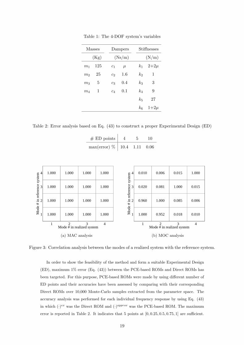
Table 1: The 4-DOF system’s variables
Masses Dampers Stiffnesses
(Kg) (Ns/m) (N/m)
m1 125 c1 µ k1 2+2µ
m2 25 c2 1.6 k2 1
m3 5 c3 0.4 k3 3
m4 1 c4 0.1 k4 9
k5 27
k6 1+2µ
Table 2: Error analysis based on Eq. (43) to construct a proper Experimental Design (ED)
# ED points 4 5 10
max(error) % 10.4 1.11 0.06
1 2 3 4
1
2
3
4
1.000
1.000
1.000
1.000
1.000
1.000
1.000
1.000
1.000
1.000
1.000
1.000
1.000
1.000
1.000
1.000
Mod
e #
in r
efer
ence
sys
tem
Mode # in realized system
(a) MAC analysis
1 2 3 4
1
2
3
4
1.000
0.960
0.020
0.010
0.952
1.000
0.081
0.006
0.018
0.085
1.000
0.015
0.010
0.006
0.015
1.000
Mod
e #
in r
efer
ence
sys
tem
Mode # in realized system
(b) MOC analysis
Figure 3: Correlation analysis between the modes of a realized system with the reference system.
In order to show the feasibility of the method and form a suitable Experimental Design
(ED), maximum 1% error (Eq. (43)) between the PCE-based ROMs and Direct ROMs has
been targeted. For this purpose, PCE-based ROMs were made by using different number of
ED points and their accuracies have been assessed by comparing with their corresponding
Direct ROMs over 10,000 Monte-Carlo samples extracted from the parameter space. The
accuracy analysis was performed for each individual frequency response by using Eq. (43)
in which (·)ex was the Direct ROM and (·)approx was the PCE-based ROM. The maximum
error is reported in Table 2. It indicates that 5 points at [0, 0.25, 0.5, 0.75, 1] are sufficient.
19
Their associated models and modal contributions are obtained to construct S and MCH2
to be prepared for making PCE.
The next step is to find a suitable basis and the associated coefficients for the polynomial
chaos expansion. In this case, since the random variable µ is uniformly distributed, the basis
of the polynomial chaos consists of Legendre polynomials. The LAR algorithm Blatman
and Sudret (2011) is employed here to calculate a sparse PCE with adaptive degree. The
efficient implementation of the LAR is available in the Matlab-based toolbox UQLab Marelli
and Sudret (2014).
To validate the approach, 10,000 Monte-Carlo samples are extracted from the parameter
space and both the true and PCE-based models are evaluated. Their accuracies are then
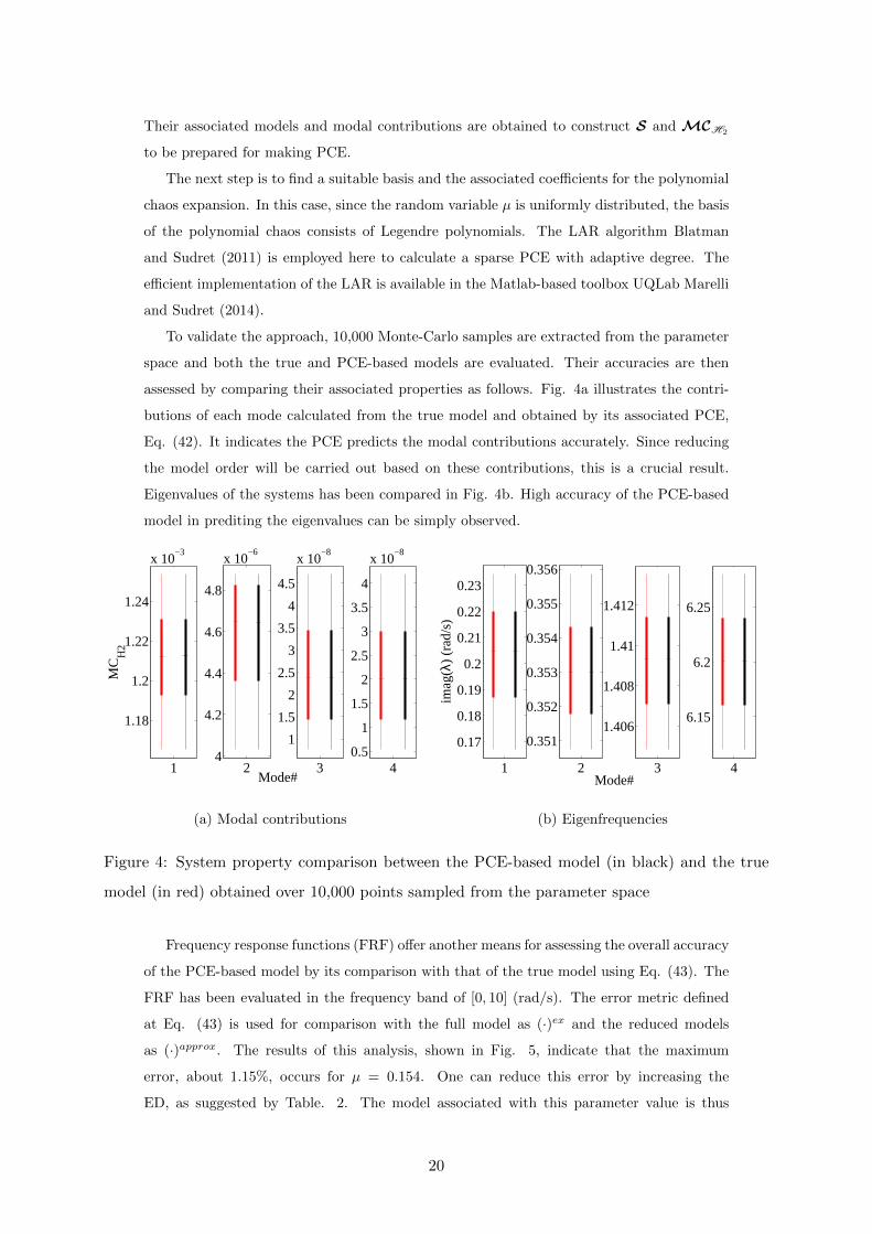
assessed by comparing their associated properties as follows. Fig. 4a illustrates the contri-
butions of each mode calculated from the true model and obtained by its associated PCE,
Eq. (42). It indicates the PCE predicts the modal contributions accurately. Since reducing
the model order will be carried out based on these contributions, this is a crucial result.
Eigenvalues of the systems has been compared in Fig. 4b. High accuracy of the PCE-based
model in prediting the eigenvalues can be simply observed.
1
1.18
1.2
1.22
1.24
x 10−3
MC
H2
24
4.2
4.4
4.6
4.8
x 10−6
3
1
1.5
2
2.5
3
3.5
4
4.5
x 10−8
40.5
1
1.5
2
2.5
3
3.5
4
x 10−8
Mode#
(a) Modal contributions
1
0.17
0.18
0.19
0.2
0.21
0.22
0.23
imag
(λ)
(rad
/s)
2
0.351
0.352
0.353
0.354
0.355
0.356
3
1.406
1.408
1.41
1.412
4
6.15
6.2
6.25
Mode#
(b) Eigenfrequencies
Figure 4: System property comparison between the PCE-based model (in black) and the true
model (in red) obtained over 10,000 points sampled from the parameter space
Frequency response functions (FRF) offer another means for assessing the overall accuracy
of the PCE-based model by its comparison with that of the true model using Eq. (43). The
FRF has been evaluated in the frequency band of [0, 10] (rad/s). The error metric defined
at Eq. (43) is used for comparison with the full model as (·)ex and the reduced models
as (·)approx. The results of this analysis, shown in Fig. 5, indicate that the maximum
error, about 1.15%, occurs for µ = 0.154. One can reduce this error by increasing the
ED, as suggested by Table. 2. The model associated with this parameter value is thus
20
selected for detailed investigation, see Fig. 6. Comparison between the eigenvalues, Fig.
6a, and FRFs of the full model and the reduced models, Fig. 6b, reveal that the proposed
method accurately predicts the reduced model. Moreover, Fig. 6c illustrates the error at
each frequency defined in Eq. (43) when (·)ex was the full true model and (·)approx was the
reduced models obtained by the modal dominancy analysis and the proposed PCE-based
method. It indicates the accuracy of the proposed method. Large error at the end of the
frequency range is due to the truncation of the last two modes. Moreover, the maximum
difference between the Direct ROM and the PCE-based model, about 1%, has been occurred
at the first resonant frequency. Since amplitudes at resonant frequencies are highly sensitive
to the damping values, the main reason for this error could be the under(over) estimation of
damping values obtained from the imaginary part of the eigenfrequencies collected in matrix
A. As mentioned, the accuracy could increase by increasing the ED size.
0 0.2 0.4 0.6 0.8 110
−1
100
101
µ
Err
or
Direct ROMPCE−based ROM
Figure 5: Error of the evaluated FRFs by changing the parameter µ
21
−0.06 −0.05 −0.04 −0.03 −0.02 −0.01 0−10
−5
0
5
10
Real(λ)
Imag(λ)
Full model
Direct ROM
PCE−based ROM
(a) Predicted eigenvalues
10−2
10−1
100
101−100
−80
−60
−40
−20
0
20
40
G(jω)[dB]
Frequency (rad/s)
Full modelDirect ROMPCE−based ROM
(b) Predicted FRF
10−2
10−1
100
10110
−4
10−2
100
102
104
Frequency (rad/s)
Err
or (
%)
Direct ROMPCE−based ROM
(c) Detailed error analysis
Figure 6: Detailed accuracy analysis for the least accurate predicted FRF among 10,000 Monte-
Carlo samples which according to Fig. 5 occurs at µ = 0.154
5.3 2-DOF system: mode veering
In this section, a 2-DOF system will be studied. This simple mechanical system, shown in
Fig. 7, presents the complex mode veering phenomenon Morand and Ohayon (1995). This
system is similar to the one studied in Amsallem and Farhat (2011); Stephen (2009). It is pa-
rameterized by the stiffness k1 = µ which follows the lognormal distribution, LN (−0.02, 0.2),
in which E [k1] = 1 and E[k21]
= 0.2. The other properties of the system are listed in Ta-
ble 3. Variation of the system’s eigenvalues, shown in Fig. 8, together with changing the
eigenvectors’s directions indicate the mode veering phenomenon.
Fig. 1 illustrates the eigenvectors of the randomly selected system together with their
associated reference ones. Fig. 1a shows the eigenvectors as they are realized for a value of
µ. As expected, they are required to transform to be similar to their corresponding reference
ones. Fig. 1b and 1c show the eigenvectors after permutation P and rotation R, respectively.
As the first step of making PCE, a proper number of samples should be chosen for the
22

ED. For this purpose, prediction accuracy of the PCE-based model has been checked over
the frequency range of [0.5, 1.8] rad/s on a large reference validation set. This set consists of
10,000 points sampled from the parameter space using the Monte-Carlo approach at which
the response of the true model has been evaluated to estimate the reference mean and
standard deviation. Then, the error (Eq.(43)) associated with the first two moments of the
PCE-based models’ responses made on experimental designs of increasing size are obtained
by comparing with the corresponding reference results. The resulting convergence curves are
given in Fig. 9. It implies that 300 points are necessary for the ED in this example, because
for larger sizes the accuracy does not improve significantly.
Therefore, since this example presents a complex problem with large COV of the parame-
ter, 300 sample points are extracted from the parameter space using the Sobol pseudorandom
sampling Sobol (1990) and the associated models are obtained to design the experiment. To
select the basis, note that X ∼ LN (λ, ξ)⇔ ln(X) ∼ N (λ, ξ), thus, the Hermite polynomial
is used as basis for ln(X).
m m
k1
c
k2
c
k3
c
q2q1
Figure 7: 2-DOF system presenting mode-veering phenomenon
Table 3: 2-DOF system’s characteristic
Characteristics m[kg] k2[N/m] k3[N/m] c[Ns/m]
value 1 0.05 1 0.001
0.6 0.8 1 1.2 1.4 1.60.8
0.9
1
1.1
1.2
µ
λ
λ1
λ2
(c)(b)
(a)
Figure 8: Mode veering phenomenon, (a) µ = 0.65, (b) µ = 1, (c) µ = 1.5
23

0 200 400 600 800 10000
5
10
15
20
25
30
# Experimental design
Err
or(m
ean)
(%
)
1st output2nd output
(a) Mean of the FRFs
0 200 400 600 800 10000
20
40
60
80
100
# Experimental design
Err
or(s
td)
(%)
1st output2nd output
(b) Standard deviation of the FRFS
Figure 9: Convergence analysis of the first two moments of the FRF to find a proper number of
points for the experimental design.
The main objective of studying this example is to show the adequacy of the method in
dealing with the complex case of mode veering phenomenon. Therefore, the 10,000 model
evaluations used to produce the convergence curves in Fig. 9 are also used to provide a
detailed validation of the performance of the PCE-based model. The results are presented as
follows. Fig. 10a shows the eigenvalues of the true model on top of those of the PCE-based
model. Their relative difference measured by
|λexi − λapproxi ||λexi |
× 100% i = 1, 2
is shown in Fig. 10b. They indicate the competence of the method in predicting the variation
of the eigenvalues when µ is varied. Moreover, using both the PCE-based model and the
true model, FRFs are evaluated and compared using Eq. (43). The results of this accuracy
analysis are shown in Fig. 11.
24
0.5 1 1.5 20.7
0.8
0.9
1
1.1
1.2
1.3
1.4
µ
λ
Exact λ1
Exact λ2
Approx. λ1
Approx. λ2
(a) Absolute values
0.5 1 1.5 20
0.5
1
1.5
2
2.5
3
µ
Err
or (
%)
λ1
λ2
(b) Relative errors
Figure 10: Predicted eigenvalues evaluated by the true model and the PCE-based model
0 5 10 15 20 250
500
1000
1500
2000
2500
Error (%)
# of
rea
lizat
ions
(a) 1st output
0 10 20 30 40 500
500
1000
1500
2000
2500
3000
3500
Error (%)
# of
rea
lizat
ions
(b) 2nd output
Figure 11: Accuracy analysis of the method by comparing the frequency response of the PCE-
based model with that of the true model evaluated by Eq. (43).
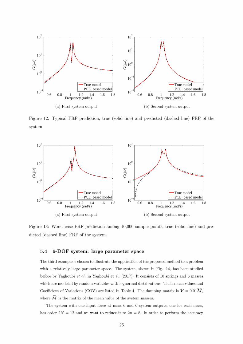
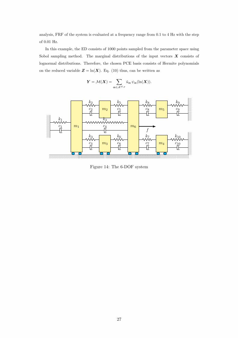
In order to visualize the accuracy of method, two realizations were considered, namely
one with a typical error, about 25% in total5, and the one with the maximum error, about
65% in total6. They are presented in Figures 12 and 13, respectively. They indicate that
even for the worst-case, the presented approach results in prediction of the system matrices
and in turn, FRFs with excellent accuracy.
5Sum of average errors at the outputs, 12%+13%=25%6Sum of maximum errors at the outputs, 22%+43%=65%
25
0.6 0.8 1 1.2 1.4 1.6 1.810
−1
100
101
102
Frequency (rad/s)
G(jω)
True modelPCE−based model
(a) First system output
0.6 0.8 1 1.2 1.4 1.6 1.810
−2
10−1
100
101
102
Frequency (rad/s)
G(jω)
True modelPCE−based model
(b) Second system output
Figure 12: Typical FRF prediction, true (solid line) and predicted (dashed line) FRF of the
system
0.6 0.8 1 1.2 1.4 1.6 1.810
−1
100
101
102
Frequency (rad/s)
G(jω)
True modelPCE−based model
(a) First system output
0.6 0.8 1 1.2 1.4 1.6 1.810
−4
10−2
100
102
Frequency (rad/s)
G(jω)
True modelPCE−based model
(b) Second system output
Figure 13: Worst case FRF prediction among 10,000 sample points, true (solid line) and pre-
dicted (dashed line) FRF of the system.
5.4 6-DOF system: large parameter space
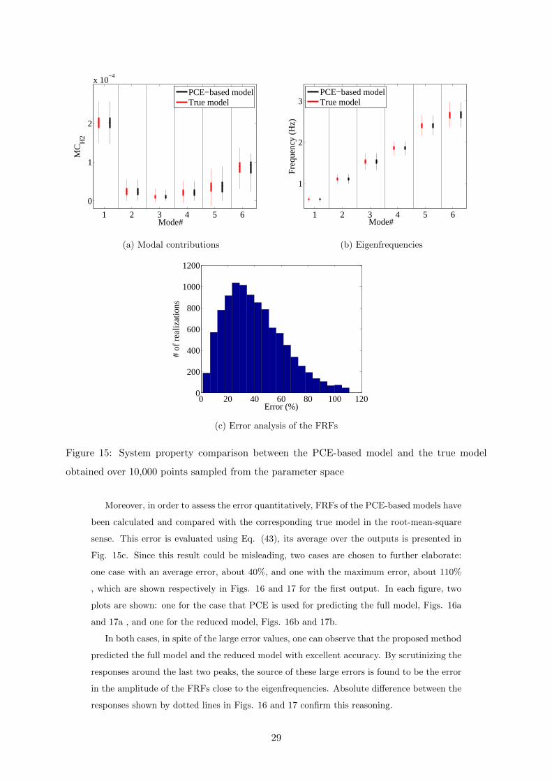
The third example is chosen to illustrate the application of the proposed method to a problem
with a relatively large parameter space. The system, shown in Fig. 14, has been studied
before by Yaghoubi et al. in Yaghoubi et al. (2017). It consists of 10 springs and 6 masses
which are modeled by random variables with lognormal distributions. Their mean values and
Coefficient of Variations (COV) are listed in Table 4. The damping matrix is V = 0.01M ,
where M is the matrix of the mean value of the system masses.
The system with one input force at mass 6 and 6 system outputs, one for each mass,
has order 2N = 12 and we want to reduce it to 2n = 8. In order to perform the accuracy
26
analysis, FRF of the system is evaluated at a frequency range from 0.1 to 4 Hz with the step
of 0.01 Hz.
In this example, the ED consists of 1000 points sampled from the parameter space using
Sobol sampling method. The marginal distributions of the input vectors X consists of
lognormal distributions. Therefore, the chosen PCE basis consists of Hermite polynomials
on the reduced variable Z = ln(X). Eq. (10) thus, can be written as
Y =M(X) =∑
α∈AM,p
uα ψα(ln(X)).
m1
m2
m3
m6
m5
m4
k1
c1
k2
c2
k3
c3
k4
c4
k5
c5
k6
c6
k7
c7
k8
c8
k9
c9
k10
c10
f
Figure 14: The 6-DOF system
27

Table 4: The 6-DOF system’s variables
Variables mean Coeff. of variation (%)
Masses [kg]
m1 50 10
m2 35 10
m3 12 10
m4 33 10
m5 100 10
m6 45 10
Stiffnesses [N/m]
k1 3000 10
k2 1725 10
k3 1200 10
k4 2200 10
k5 1320 10
k6 1330 10
k7 1500 10
k8 2625 10
k9 1800 10
k10 850 10
The LAR algorithm has been employed to build sparse PCEs with adaptive degree. Since
the dimension of the input parameter space is large, to reduce the unknown coefficients of the
PCEs and avoid the curse of dimensionality, a hyperbolic truncation with q-norm of 0.7 was
used before the LAR algorithm. Besides, only polynomials up to rank 2 were selected here
(i.e. polynomials that depend at most on 2 of the 16 parameters). It should be mentioned
that all the PCEs used for the surrogate model have eventually maximum degrees less than
10.
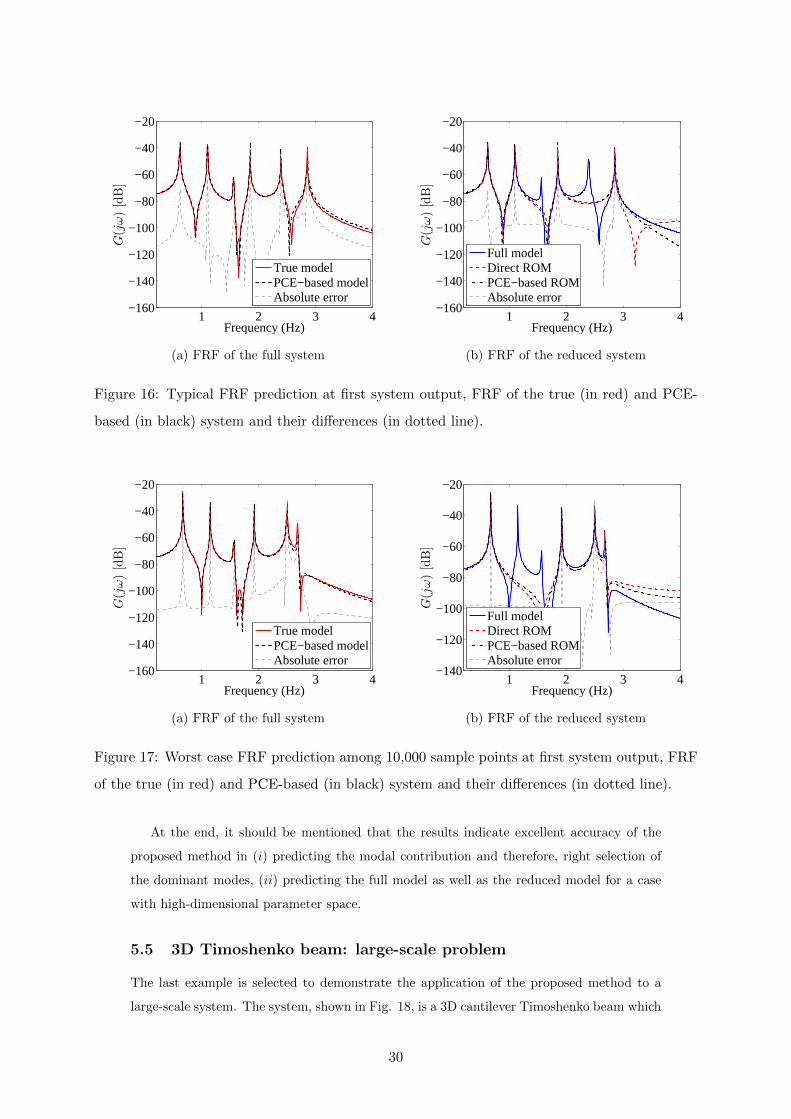
In order to assess the accuracy of the PCE-based model in estimating various quantities of
interests, 10,000 points sampled from the parameter space by using Monte-Carlo sampling at
which both the true and the PCE-based models are evaluated and their associated properties
have been compared in Fig. 15. Fig. 15a illustrates the contributions of each mode calculated
from the true model and obtained by its associated PCE, Eq. (42). Eigenvalues of the systems
have been compared in Fig. 15b.
28
1 2 3 4 5 6
0
1
2
x 10−4
MC
H2
PCE−based modelTrue model
Mode#
(a) Modal contributions
1 2 3 4 5 6
1
2
3
Fre
quen
cy (
Hz)
PCE−based modelTrue model
Mode#
(b) Eigenfrequencies
0 20 40 60 80 100 1200
200
400
600
800
1000
1200
Error (%)
# of
rea
lizat
ions
(c) Error analysis of the FRFs
Figure 15: System property comparison between the PCE-based model and the true model
obtained over 10,000 points sampled from the parameter space
Moreover, in order to assess the error quantitatively, FRFs of the PCE-based models have
been calculated and compared with the corresponding true model in the root-mean-square
sense. This error is evaluated using Eq. (43), its average over the outputs is presented in
Fig. 15c. Since this result could be misleading, two cases are chosen to further elaborate:
one case with an average error, about 40%, and one with the maximum error, about 110%
, which are shown respectively in Figs. 16 and 17 for the first output. In each figure, two
plots are shown: one for the case that PCE is used for predicting the full model, Figs. 16a
and 17a , and one for the reduced model, Figs. 16b and 17b.
In both cases, in spite of the large error values, one can observe that the proposed method
predicted the full model and the reduced model with excellent accuracy. By scrutinizing the
responses around the last two peaks, the source of these large errors is found to be the error
in the amplitude of the FRFs close to the eigenfrequencies. Absolute difference between the
responses shown by dotted lines in Figs. 16 and 17 confirm this reasoning.
29
1 2 3 4−160
−140
−120
−100
−80
−60
−40
−20
Frequency (Hz)
G(jω)[dB]
True modelPCE−based modelAbsolute error
(a) FRF of the full system
1 2 3 4−160
−140
−120
−100
−80
−60
−40
−20
Frequency (Hz)
G(jω)[dB]
Full modelDirect ROMPCE−based ROMAbsolute error
(b) FRF of the reduced system
Figure 16: Typical FRF prediction at first system output, FRF of the true (in red) and PCE-
based (in black) system and their differences (in dotted line).
1 2 3 4−160
−140
−120
−100
−80
−60
−40
−20
Frequency (Hz)
G(jω)[dB]
True modelPCE−based modelAbsolute error
(a) FRF of the full system
1 2 3 4−140
−120
−100
−80
−60
−40
−20
Frequency (Hz)
G(jω)[dB]
Full modelDirect ROMPCE−based ROMAbsolute error
(b) FRF of the reduced system
Figure 17: Worst case FRF prediction among 10,000 sample points at first system output, FRF
of the true (in red) and PCE-based (in black) system and their differences (in dotted line).
At the end, it should be mentioned that the results indicate excellent accuracy of the
proposed method in (i) predicting the modal contribution and therefore, right selection of
the dominant modes, (ii) predicting the full model as well as the reduced model for a case
with high-dimensional parameter space.
5.5 3D Timoshenko beam: large-scale problem
The last example is selected to demonstrate the application of the proposed method to a
large-scale system. The system, shown in Fig. 18, is a 3D cantilever Timoshenko beam which
30
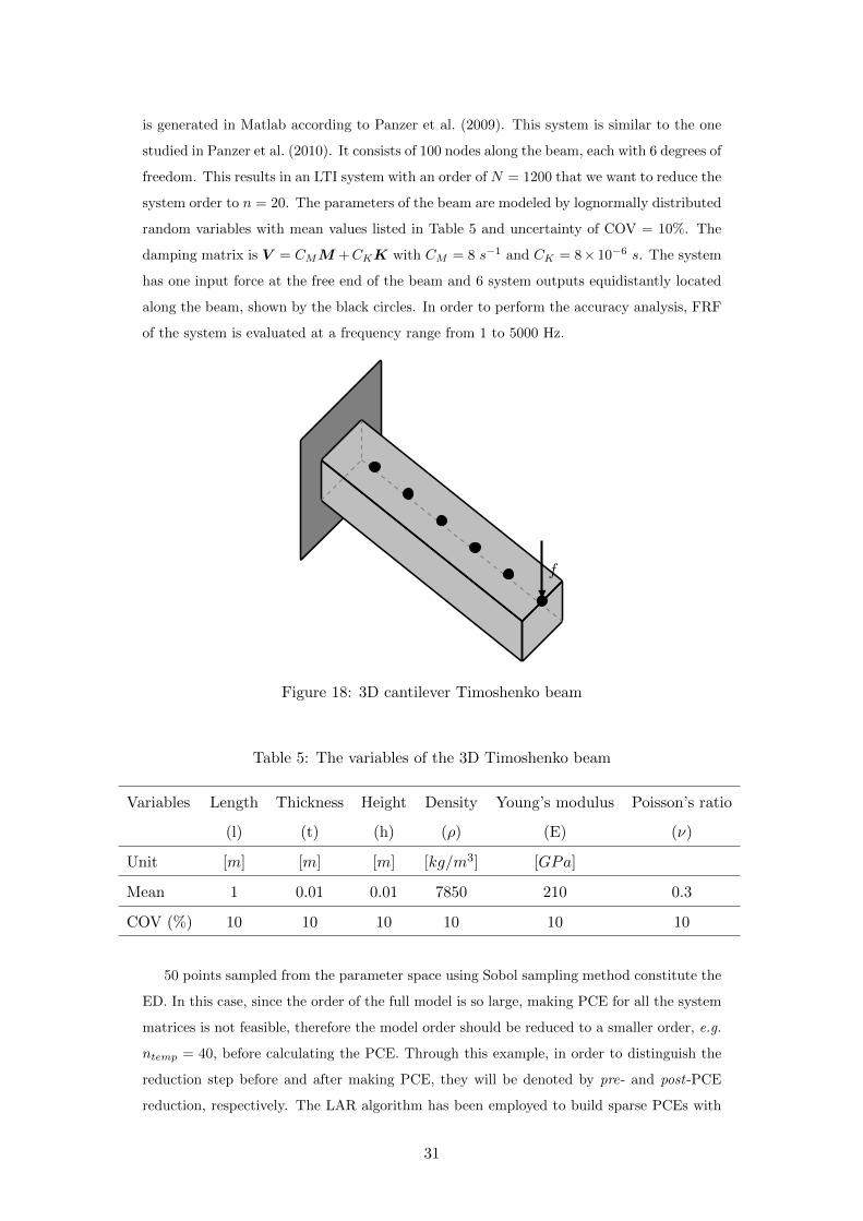
is generated in Matlab according to Panzer et al. (2009). This system is similar to the one
studied in Panzer et al. (2010). It consists of 100 nodes along the beam, each with 6 degrees of
freedom. This results in an LTI system with an order of N = 1200 that we want to reduce the
system order to n = 20. The parameters of the beam are modeled by lognormally distributed
random variables with mean values listed in Table 5 and uncertainty of COV = 10%. The
damping matrix is V = CMM +CKK with CM = 8 s−1 and CK = 8× 10⁻⁶ s. The system
has one input force at the free end of the beam and 6 system outputs equidistantly located
along the beam, shown by the black circles. In order to perform the accuracy analysis, FRF
of the system is evaluated at a frequency range from 1 to 5000 Hz.
f
Figure 18: 3D cantilever Timoshenko beam
Table 5: The variables of the 3D Timoshenko beam
Variables Length Thickness Height Density Young’s modulus Poisson’s ratio
(l) (t) (h) (ρ) (E) (ν)
Unit [m] [m] [m] [kg/m3] [GPa]
Mean 1 0.01 0.01 7850 210 0.3
COV (%) 10 10 10 10 10 10
50 points sampled from the parameter space using Sobol sampling method constitute the
ED. In this case, since the order of the full model is so large, making PCE for all the system
matrices is not feasible, therefore the model order should be reduced to a smaller order, e.g.
ntemp = 40, before calculating the PCE. Through this example, in order to distinguish the
reduction step before and after making PCE, they will be denoted by pre- and post-PCE
reduction, respectively. The LAR algorithm has been employed to build sparse PCEs with
31
adaptive degree. PCA has been performed over the C matrix and the dominant components
are selected such that∑NY
i=1 λCOVi = 0.99
∑NY
i=1 λCOVi here λCOV are the eigenvalues of the
covariance matrix, see Eq. (15). This truncation reduced the number of random outputs
from 240 × 2 to 6 components.
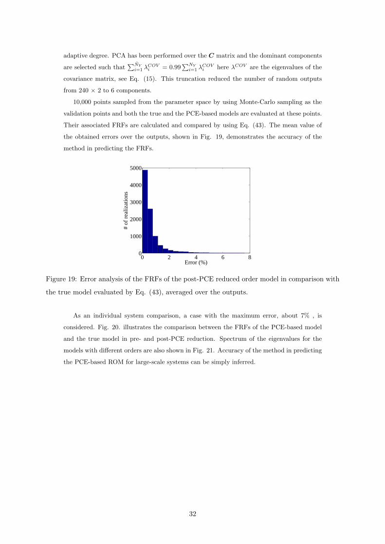
10,000 points sampled from the parameter space by using Monte-Carlo sampling as the
validation points and both the true and the PCE-based models are evaluated at these points.
Their associated FRFs are calculated and compared by using Eq. (43). The mean value of
the obtained errors over the outputs, shown in Fig. 19, demonstrates the accuracy of the
method in predicting the FRFs.
0 2 4 6 80
1000
2000
3000
4000
5000
Error (%)
# of
rea
lizat
ions
Figure 19: Error analysis of the FRFs of the post-PCE reduced order model in comparison with
the true model evaluated by Eq. (43), averaged over the outputs.
As an individual system comparison, a case with the maximum error, about 7% , is
considered. Fig. 20. illustrates the comparison between the FRFs of the PCE-based model
and the true model in pre- and post-PCE reduction. Spectrum of the eigenvalues for the
models with different orders are also shown in Fig. 21. Accuracy of the method in predicting
the PCE-based ROM for large-scale systems can be simply inferred.
32

101
102
103−200
−150
−100
−50
0
Frequency (Hz)
G(jω)[dB]
True modelPCE−based model
(a) FRF of the full system
101
102
103−200
−150
−100
−50
0
Frequency (Hz)
G(jω)[dB]
Full modelDirect ROMPCE−based ROM
(b) FRF of the reduced system
Figure 20: Worst case FRF prediction among 10,000 sample points at first system output,
evaluated by true model (in red) and PCE-based model (in black).
−108
−107
−106
−105
−104
−103
−102
−101
−100
−1.5
−1
−0.5
0
0.5
1
1.5x 10
5
−log(−Real(λ))
Imag(λ)
Full modelTrue model: Pre−PCE red.PCE model: Pre−PCE red.True model: Post−PCE red.PCE model: Post−PCE red.
Figure 21: Eigenvalue spectrum of the systems realized at the parameter set with the maximum
average error.
6 Concluding remarks
In this paper, a PCE-based parametric model reduction method for dynamic systems has
been developed. This method consists of a PCE-based surrogate model for state-space models
together with a PCE-based modal dominancy method to reduce the model order, if required.
For this purpose, a method has been proposed based on QR factorization to fix the eigenvec-
tors of the modes with coalescent eigenvalues. Moreover, a new correlation metric has been
introduced for mode tracking, which was shown to be effective to resolve the spatial aliasing
phenomenon in cases with few number of sensors. The problem of the curse of dimensionality
33
of PCEs in cases with large parameter spaces was alleviated by employing the LAR algo-
rithm to build sparse PCEs together with an adaptive degree strategies. In order to reduce
the number of random outputs in large-scale systems with high model orders two solutions
were proposed: first, reduce the model order to an intermediate level before making PCE
and second, use of PCA while making PCE. Successful application of the proposed method
to four case studies indicate its capability in accurately predicting the modal contributions,
eigenvalues, and more importantly, full and reduced order systems. The case studies are se-
lected such that each of them resembles a frequently occurred challenge in complex systems,
such as mode veering, large parameter space and large-scale systems.
Acknowledgments
The authors would like to appreciate financial support from Iran National Elite Foundation.
References
Allemang, R. J. (2003). The modal assurance criterion–twenty years of use and abuse. Sound
vibration 37 (8), 14–23.
Amsallem, D. and C. Farhat (2008). Interpolation method for adapting reduced-order models
and application to aeroelasticity. AIAA journal 46, 1803–1813.
Amsallem, D. and C. Farhat (2011). An online method for interpolating linear parametric
reduced-order models. SIAM J. Sci. Comput. 33, 2169–2198.
Antoulas, A. C. (2005). Approximation of large-scale dynamical systems, Volume 6. Siam.
Antoulas, A. C., D. C. Sorensen, and S. Gugercin (2001). A survey of model reduction
methods for large-scale systems. Contemporary mathematics 280, 193–220.
Avitabile, P. and J. O’Callahan (2009). Efficient techniques for forced response involving
linear modal components interconnected by discrete nonlinear connection elements. Mech.
Syst. Signal Pr. 23, 45–67.
Baur, U., P. Benner, A. Greiner, J. G. Korvink, J. Lienemann, and C. Moosmann (2011).
Parameter preserving model order reduction for MEMS applications. Math. Comp. Model
Dyn. 17, 297–317.
Benner, P., S. Gugercin, and K. Willcox (2013). A survey of model reduction methods for
parametric systems.
Berveiller, M., B. Sudret, and M. Lemaire (2006). Stochastic finite element: a non intrusive
approach by regression. Eur. J. Comput. Mech. 15, 81–92.
34
Blatman, G. and B. Sudret (2008). Sparse polynomial chaos expansions and adaptive stochas-
tic finite elements using a regression approach. Comptes Rendus Mecanique 336, 518–523.
Blatman, G. and B. Sudret (2010). An adaptive algorithm to build up sparse polynomial
chaos expansions for stochastic finite element analysis. Probabilist. Eng. Mech. 25, 183–
197.
Blatman, G. and B. Sudret (2011). Adaptive sparse polynomial chaos expansion based on
least angle regression. J. Comput. Phys. 230, 2345–2367.
Blatman, G. and B. Sudret (2013). Sparse polynomial chaos expansions of vector-valued re-
sponse quantities. In G. Deodatis (Ed.), Proc. 11th Int. Conf. Struct. Safety and Reliability
(ICOSSAR’2013), New York, USA.
Bogoevska, S., M. Spiridonakos, E. Chatzi, E. Dumova-Jovanoska, and R. Hoffer (2017).
A data-driven diagnostic framework for wind turbine structures: A holistic approach.
Sensors 17, 720.
Dertimanis, V., M. Spiridonakos, and E. Chatzi (2017). Data-driven uncertainty quantifica-
tion of structural systems via b-spline expansion. Computers & Structures.
Efron, B., T. Hastie, I. Johnstone, R. Tibshirani, et al. (2004). Least angle regression. Ann.
Stat. 32, 407–499.
Frangos, M., Y. Marzouk, K. Willcox, and B. van Bloemen Waanders (2010). Surrogate and
reduced-order modeling: A comparison of approaches for large-scale statistical inverse
problems. Large-Scale Inverse Problems and Quantification of Uncertainty 123149.
Fricker, T. E., J. E. Oakley, N. D. Sims, and K. Worden (2011). Probabilistic uncertainty
analysis of an FRF of a structure using a Gaussian process emulator. Mech. Syst. Signal
Pr. 25, 2962–2975.
Ghanem, R. and D. Ghiocel (1998). Stochastic seismic soil-structure interaction using the
homogeneous chaos expansion. In Proc. 12th ASCE Engineering Mechanics Division Con-
ference, La Jolla, California, USA.
Ghanem, R. G. and P. D. Spanos (2003). Stochastic finite elements: a spectral approach.
Courier Corporation.
Ghiocel, D. and R. Ghanem (2002). Stochastic finite element analysis of seismic soil-structure
interaction. J. Eng. Mech. 128, 66–77.
Gilli, L., D. Lathouwers, J. Kloosterman, T. van der Hagen, A. Koning, and D. Rochman
(2013). Uncertainty quantification for criticality problems using non-intrusive and adaptive
polynomial chaos techniques. Ann. Nucl. Energy 56, 71–80.
35

Hastie, T., J. Taylor, R. Tibshirani, G. Walther, et al. (2007). Forward stagewise regression
and the monotone lasso. Electron. J. Stat. 1, 1–29.
Jones, D. R., M. Schonlau, and W. J. Welch (1998). Efficient global optimization of expensive
black-box functions. J. Global Optim. 13, 455–492.
Kersaudy, P., B. Sudret, N. Varsier, O. Picon, and J. Wiart (2015). A new surrogate modeling
technique combining Kriging and polynomial chaos expansions–application to uncertainty
analysis in computational dosimetry. J. Comput. Phys. 286, 103–117.
Kim, T. (2015). Surrogate model reduction for linear dynamic systems based on a frequency
domain modal analysis. Comput. Mech. 56, 709–723.
Kim, T. (2016). Parametric model reduction for aeroelastic systems: Invariant aeroelastic
modes. J. Fluid Struct. 65, 196–216.
Kim, T. S. and Y. Y. Kim (2000). MAC-based mode-tracking in structural topology opti-
mization. Comput Struct 74, 375–383.
Knio, O. M., H. N. Najm, R. G. Ghanem, et al. (2001). A stochastic projection method for
fluid flow: I. basic formulation. J. Comput. Phys. 173, 481–511.
Laub, A. J. (2005). Matrix analysis for scientists and engineers. Philadelphia, PA, USA:
SIAM.
Liu, T., C. Zhao, Q. Li, and L. Zhang (2012). An efficient backward Euler time-integration
method for nonlinear dynamic analysis of structures. Comput. Struct. 106, 20–28.
Lohmann, B. and R. Eid (2007). Efficient order reduction of parametric and nonlinear
models by superposition of locally reduced models. In Methoden und Anwendungen der
Regelungstechnik. Erlangen-Munchener Workshops, pp. 27–36.
Mai, C., M. Spiridonakos, E. Chatzi, and B. Sudret (2016). Surrogate modelling for stochastic
dynamical systems by combining nonlinear autoregressive with exogenous input models
and polynomial chaos expansions. Int. J Uncertain Quantif 6.
Manan, A. and J. Cooper (2010). Prediction of uncertain frequency response function bounds
using polynomial chaos expansion. J. Sound Vib. 329, 3348–3358.
Marelli, S. and B. Sudret (2014). UQLab: a framework for uncertainty quantification in
matlab. In Vulnerability, Uncertainty, and Risk: Quantification, Mitigation, and Manage-
ment, pp. 2554–2563.
Marelli, S. and B. Sudret (2015). UQLab user manual–polynomial chaos expansions. Techni-
cal report, Report UQLab-V0.9-104, Chair of Risk, Safety & Uncertainty Quantification,
ETH Zurich.
36

Morand, H. and R. Ohayon (1995). Fluid structure interaction. ZAMM Z. Angew. Math.
Mech 76, 376–376.
Panzer, H., J. Hubele, R. Eid, and B. Lohmann (2009). Generating a parametric finite
element model of a 3d cantilever timoshenko beam using matlab. Tech. reports on aut.
control, Inst. Aut. Control, TU Munchen.
Panzer, H., J. Mohring, R. Eid, and B. Lohmann (2010). Parametric model order reduction
by matrix interpolation. at-Automatisierungstechnik 58, 475–484.
Rahrovani, S., M. K. Vakilzadeh, and T. Abrahamsson (2014). Modal dominancy analysis
based on modal contribution to frequency response function H2-norm. Mech. Syst. Signal
Pr. 48, 218–231.
Schobi, R., B. Sudret, and J. Wiart (2015). Polynomial-chaos-based Kriging. Int. J. Uncer-
tainty Quantification 5, 171–193.
Schueller, G. and H. Pradlwarter (2009). Uncertain linear systems in dynamics: Retrospec-
tive and recent developments by stochastic approaches. Eng. Struct. 31, 2507–2517.
Sobol, I. (1990). Quasi-monte carlo methods. Progress in Nuclear Energy 24, 55–61.
Soize, C. and R. Ghanem (2004). Physical systems with random uncertainties: chaos repre-
sentations with arbitrary probability measure. SIAM J. Sci. Comput. 26, 395–410.
Stephen, N. (2009). On veering of eigenvalue loci. J. Vib. Acoust. 131, 054501.
Sudret, B. (2007). Uncertainty propagation and sensitivity analysis in mechanical models –
contributions to structural reliability and stochastic spectral methods. Technical report.
Habilitation a diriger des recherches, Universite Blaise Pascal, Clermont-Ferrand, France
(229 pages).
Tak, M. and T. Park (2013). High scalable non-overlapping domain decomposition method
using a direct method for finite element analysis. Comput. Methods Appl. Mech. En-
grg. 264, 108–128.
Wiener, N. (1938). The homogeneous chaos. Amer. J. Math., 897–936.
Xiu, D. and G. E. Karniadakis (2002). The Wiener–Askey polynomial chaos for stochastic
differential equations. SIAM J. Sci. Comput. 24, 619–644.
Yaghoubi, V. and T. Abrahamsson (2014). The modal observability correlation as a modal
correlation metric. In Topics in Modal Analysis, Volume 7, pp. 487–494. Springer.
Yaghoubi, V., T. Abrahamsson, and E. A. Johnson (2016). An efficient exponential predictor-
corrector time integration method for structures with local nonlinearity. Eng. Struct. 128,
344 – 361.
37

Yaghoubi, V., S. Marelli, B. Sudret, and T. Abrahamsson (2017). Sparse polynomial chaos
expansions of frequency response functions using stochastic frequency transformation.
Probab. Eng. Mech. 48, 39 – 58.
Yaghoubi, V., M. K. Vakilzadeh, and T. Abrahamsson (2015). A parallel solution method
for structural dynamic response analysis. In Dynamics of Coupled Structures, Volume 4,
pp. 149–161. Springer.
Yang, J., B. Faverjon, H. Peters, and N. Kessissoglou (2015). Application of polynomial chaos
expansion and model order reduction for dynamic analysis of structures with uncertainties.
Procedia IUTAM 13, 63–70.
38