reducing effects of bad data using variance based joint
TRANSCRIPT

J Sci Comput (2019) 78:94–120
https://doi.org/10.1007/s10915-018-0754-2
Reducing Effects of Bad Data Using Variance Based Joint
Sparsity Recovery
Anne Gelb1 · Theresa Scarnati2,3
Received: 19 December 2017 / Revised: 30 April 2018 / Accepted: 30 May 2018 /
Published online: 13 June 2018
© Springer Science+Business Media, LLC, part of Springer Nature 2018
Abstract Much research has recently been devoted to jointly sparse (JS) signal recovery
from multiple measurement vectors using �2,1 regularization, which is often more effective
than performing separate recoveries using standard sparse recovery techniques. However, JS
methods are difficult to parallelize due to their inherent coupling. The variance based joint
sparsity (VBJS) algorithm was recently introduced in Adcock et al. (SIAM J Sci Comput,
submitted). VBJS is based on the observation that the pixel-wise variance across signals con-
vey information about their shared support, motivating the use of a weighted �1 JS algorithm,
where the weights depend on the information learned from calculated variance. Specifically,
the �1 minimization should be more heavily penalized in regions where the corresponding
variance is small, since it is likely there is no signal there. This paper expands on the original
method, notably by introducing weights that ensure accurate, robust, and cost efficient recov-
ery using both �1 and �2 regularization. Moreover, this paper shows that the VBJS method
can be applied in situations where some of the measurement vectors may misrepresent the
unknown signals or images of interest, which is illustrated in several numerical examples.
Keywords Multiple measurement vectors · Joint sparsity · Image reconstruction · False
data injections
Mathematics Subject Classification 65F22 · 65K10 · 68U10
Anne Gelb’s work is supported in part by the Grants NSF-DMS 1502640, NSF-DMS 1732434, and AFOSR
FA9550-15-1-0152. Approved for public release. PA Approval #:[88AWB-2017-6162].
B Anne Gelb
Theresa Scarnati
1 Department of Mathematics, Dartmouth College, Hanover, USA
2 School of Mathematical and Statistical Sciences, Arizona State University, Tempe, USA
3 Air Force Research Laboratory, Wright-Patterson AFB, Dayton, USA
123
J Sci Comput (2019) 78:94–120 95
1 Introduction
Recovering sparse signals and piecewise smooth functions from under-sampled and noisy
data has been a heavily investigated topic over the past decade. Typical algorithms minimize
the �1 norm of an approximation of a sparse feature (e.g. wavelets, gradients, or edges) of the
solution so that the reconstructed solution will preserve sparsity in its corresponding sparse
domain. A weighted �1 reconstruction algorithm was introduced in [8] to reconcile the dif-
ference between the “true” sparsity �0 norm and the surrogate �1. Sparse signal recovery
was accomplished by a solving a sequence of weighted �1 minimization problems, with the
weights iteratively updated at each step. As was demonstrated there, updating the weights
yielded successively improved estimations of the non-zero coefficient locations, and conse-
quently relaxes standard sampling rate requirements for sparse signal recovery. An adjustment
for the weight calculation was proposed in [10] resulting in an improvement to the iterative
reweighting algorithm. An adaptively weighted total variation (TV) regularization algorithm,
where the spatially adaptive weights were based on the difference of values between neigh-
boring pixels, was introduced in [25]. A different weighting technique was developed in [9]
to reduce the staircase effect of TV regularization. An adaptive function was used along with
new parameters to balance the trade off between penalizing discontinuities and recovering
sharp edges. While the method accomplishes the goal of allowing smooth transitions without
reducing sharp edges, the mathematical formulation is challenging and uniqueness is not
guaranteed. Further weighted �1 literature can be found at [8–10,25,39,40] and references
therein.
In many inverse problems, it may be possible to acquire multiple measurement vec-
tors (MMVs) of the unknown signal or image, [2,11,12,16–18,24,30]. MMV collection is
especially useful when trying to recover solutions of an underdetermined system when the
MMVs have the same, but unknown, sparsity structure. Techniques exploiting this type of
commonality, referred to as joint sparsity (JS) methods, can be developed by extending the
commonly used single measurement vector (SMV) algorithms for sparse solutions, [12].
Additional examples of this can be found in [11,21,33,35,37] and references therein. In
particular, jointly sparse vectors are often recovered using the popular �2,1 minimization,
[11,14,31,42,44], which was thoroughly analyzed in [16,17]. Conditions for guaranteeing
improvements over SMV were determined for a class of MMV techniques in [16] and more-
over, it was shown in [17] that under mild conditions the probability of not recovering a sparse
vector with high probability (based on a chosen threshold) using �2,1 regularization decays
exponentially with the increase of measurements. Various algorithms are used to implement
�2,1 regularization, including the alternating direction method of multipliers (ADMM), split
Bregman, joint-OMP, and “reduce-and-boost”, [26,34,42]. An algorithm is typically cho-
sen to yield the most efficiency for the particular problem at hand (for example, based on
problem complexity). In this paper we use ADMM, and note that while other methods may
yield faster convergence for our chosen examples, in general �2,1 regularization techniques
are inherently coupled, making them difficult to parallelize.
While much work has been done on designing weighted �p (specifically �1) reconstruction
methods for SMV, and in constructing joint sparsity MMV methods using the �2,1 norm, there
has been less work devoted to improving MMV through weighted �p minimization. Three
notable investigations include: (1) [31], where the SMV weights were adapted from those in
[8] to �2,1 minimization for the problem of multi-channel electrocardiogram signal recovery.
Although the technique enhances the sparseness of the solution and reduce the number of
measurements required for accurate recovery, it requires hand tuning of parameters. (2) [44],
123
96 J Sci Comput (2019) 78:94–120
where a weighted �2,1 minimization algorithm is used for direction of arrival estimation,
high resolution radar imaging and other sparse recovery related problems using random
measurement matrices. The singular value decomposition is used to exploit the relationship
between the signal subspace and the noise subspace for designing the weights. (3) [18],
where a shape-adaptive jointly sparse classification method for hyperspectral imaging was
developed. We note that all of these developments were problem specific, and not easily
adapted for general sparse signal recovery.
In this investigation we propose using the variance based joint sparsity (VBJS) method
for MMV, introduced in [1]. The VBJS technique exploits the idea that the variance across
multi-measurement vectors that are jointly sparse should be sparse in the sparsity domain
of the underlying signal or image, an idea first proposed in [15] for the purpose of edge
detection and localization. The weights used for the weighted �1 regularization term are
essentially reciprocals of this variance (with a threshold built in to ensure no division by
zero), with the idea being that the �1 term should be heavily penalized when the variance is
small, but should not influence the solution as much when the variance is large. Presumably,
the large variance indicates support of the image or signal in the sparse domain. One of the
main advantages of VBJS is that it is easily parallelized. In particular, it was shown in [1] that
VBJS is consistently more computationally efficient than �2,1 regularization algorithms when
using standard black box solvers. In this investigation we improve on the VBJS algorithm
by designing weights that reduce the parametric dependence on the reconstruction, making
it more amenable to a variety of other applications not considered in [1]. Specifically, the
VBJS can now be used in situations where some measurement vectors may misrepresent the
unknown function of interest. In contrast, such “rogue” data may wield undue influence on
the reconstruction of piecewise smooth solutions when using the standard �2,1 approach. The
original VBJS approach does not adequately account for false data in the weight design, so
much more parameter tuning would be needed. False data problems appear in applications
including state estimation of electrical power grids, [23], large scale sensor network esti-
mation, [41], synthetic aperture radar (SAR) automated target recognition (ATR), [20], and
many others, [43,45]. False data may be purposefully injected into these systems to decrease
the performance of automated detection algorithms. In other situations, misrepresentations
of data occur due to human error or environmental issues effecting the measurements. For
example, in SAR ATR it is often the case that targets are obscured by their surroundings (trees)
or by enemies (meshes placed over the targets). Also, additional parts may be taken off or
added to targets, corrupting measurement data, [20]. As part of our reconstruction algorithm,
we include a numerically efficient comparative measurement of the measurement vectors,
which allow us to appropriately disregard rogue data and improve our overall reconstruction.
Our proposed VBJS technique offers several advantages: (1) Our method is (essen-
tially) non-parametric so that regularization parameters need not be hand tuned; (2) We
take advantage of the joint sparsity information available in the MMV setup, thus improv-
ing reconstruction accuracy while decreasing sampling rates, independent of application; (3)
With some sharpness reduction, our weights allow us to use the �2 norm, which is much more
cost efficient; (4) Our method mitigates the effects of rogue data. Finally, as noted above,
the VBJS algorithm is easily parallelizable, so even when using the weighted �1 norm, it is
much more efficient than when the �2,1 norm is used.
The rest of the paper is organized as follows: In Sect. 2 we define joint sparsity for multi-
measurement vectors and provide details for the standard �2,1 regularization approach used
to recover sparse signals. In Sect. 3 we describe the variance based joint sparsity (VBJS)
approach, initially developed in [1], and demonstrate how weights should be constructed to
reduce the impact of false information. We also propose a technique to choose the “best”
123

J Sci Comput (2019) 78:94–120 97
solution from the set of possible solution vectors that can be recovered from the VBJS method,
so that we do not have to compute each vector in the solution space. In Sect. 4 we prove
that the alternating direction method of multipliers (ADMM) can be applied to the weighted
�1 minimization. We also show how the VBJS method can be efficiently computed for the
weighted �2 norm. Section 5 provides some numerical results for sparse signal recovery and
one and two dimensional images. Some concluding remarks are given in Sect. 6.
2 Preliminaries
Consider a piecewise smooth function f (x) on [a, b]. We seek to recover f ∈ RN , where
each element of f is given as fi = f (xi ), i = 1, . . . , N , with
xi = a + Δx(i − 1), (2.1)
and Δx = b−aN
. We note that xi are chosen to be uniform for simplicity of numerical
experiments and is not required for our algorithm.
Since the underlying function f is piecewise smooth, it is sparse in its corresponding edge
domain. Formally we have:
Definition 1 [11,13] A vector p ∈ RN is s-sparse for some 1 ≤ s ≤ N if
|| p||0 = |supp( p)| ≤ s.
In our case, p corresponds to the edge vector of f at the set of grid points in (2.1).
Suppose we acquire J data vectors, y j ∈ CM , as
y j = A j ( f ) + η j , j = 1, . . . , J. (2.2)
Here A j : RN → C
M is a forward operator (often defined as a square (N = M), orthogonal
matrix for simplicity) and
η j ∈ CM , j = 1, . . . , J, (2.3)
model J Gaussian noise vectors.
Due to the sparsity in the edge domain, �1 regularization provides an effective means
for reconstructing f given any of the J noisy data vectors. Specifically, we compute the
unconstrained optimization problem
fj = argmin
g
{
1
2||A j g − y j ||22 + μ||Lg||1
}
, j = 1, . . . , J, (2.4)
where μ is the �1 regularization parameter. In our experiments we often sample μ from a
uniform distribution for all calculations of fj
to simulate the ad-hoc procedure for selecting
typical regularization parameters. The sparsifying operator, L, is designed so that the chosen
solution is sparse in the edge domain. In this investigation we choose L to be the mth order
polynomial annihilation (PA) [3,4], and note that when m = 1 the method is equivalent to
using total variation (TV).1 To solve (2.4) we use the traditional alternating direction method
of multipliers (ADMM) algorithm [19,22,36].
1 Although there are subtle differences in the derivations and normalizations, the PA transform can be thought
of as higher order total variation (HOTV). Because part of our investigation discusses parameter selection,
which depends explicitly on ||L f ||, we will exclusively use the PA transform as it appears in [3] so as to avoid
any confusion. Explicit formulations for the PA transform matrix can be found in [3]. We also note that the
method can be easily adapted for other sparsifying transformations.
123
98 J Sci Comput (2019) 78:94–120
As shown in Fig. 1(left), assuming that the model in (2.2) is correct, any of the reconstructed
fj
(which we will refer to as the single measurement vector (SMV) reconstruction) should
adequately approximate the underlying function f or any desired features of it. However,
this may be impossible due to undersampling, noise, or bad information. Intuitively, using
the redundant data from part of or all of the available data sets in (3.1) should lead to a better
reconstruction algorithm. Indeed, many techniques have been developed to recover images
from such multiple measurement vectors (MMV), [2,11,12,16–18,24,30]. In our case the
underlying function f is sparse in the edge domain, and so the collected set of recovered
vectors is jointly sparse in the edge domain. The formal definition of joint sparsity is given
by
Definition 2 We say that
P =[
p1 p2 · · · pJ]
∈ RN×J
is s-joint sparse if
||P ||2,0 =
∣
∣
∣
∣
∣
∣
J⋃
j=1
supp( p j )
∣
∣
∣
∣
∣
∣
≤ s,
where each p j is s-sparse according to Definition 1.
For the variance based joint sparsity method in Algorithm 1, we also will assume that
supp( p1) ≈ supp( p2) ≈ · · · ≈ supp( pJ ), (2.5)
that is, the joint sparsity of the vectors does not greatly exceed the sparsity of each individual
vector.
To exploit the joint sparsity of the system, �2,1 regularization is often applied, [11,32,42,
44]. Essentially, each vector is assumed to be sparse in its sparsity domain (e.g. edge domain),
which motivates minimizing the �1 norm of each column. The “jointness” is accomplished by
minimizing the �2 norm of each row (spatial elements). The general joint sparsity technique
using �2,1 regularization is [32]
f ={
argminz∈RN×J
||Lz||2,1 subject to Az = Y
}
, (2.6)
where L is the sparsifying transform matrix (here the PA transform of order m),
Y = [ y1 y2 · · · yJ ] ∈ RM×J and A = A1 = · · · = AJ . The solution f =
[ f1
f2 · · · f
J ] ∈ RN×J contains estimates for each measurement y j , j = 1, . . . , J .
It has been shown, both theoretically and in practice, that (2.6) yields improved approxima-
tions to each reconstruction in (2.4), [11,31,44].
Note that (2.6) is typically solved using optimization techniques such as the ADMM,
focal underdetermined system solvers (FOCUSS) and matching pursuit algorithms, [12].2
As demonstrated in Fig. 1(middle), the joint sparsity approach using �2,1 regularization is
effective in cases where the data vectors are somewhat predictable, that is, when each mea-
surement vector is determined from (2.2), and A j is known. However, it is often the case
when some of the acquired data do not have known sources. Worse, the information can be
deliberately misleading, so that we assume we are acquiring y j but in fact a completely dif-
ferent data set is obtained. We will refer to such a data set as a “rogue” vector. Figure 1(right)
2 We used the Matlab code provided in [14,42] when implementing (2.6).
123

J Sci Comput (2019) 78:94–120 99
Fig. 1 Sparse vector of uniformly distributed values on [0, 1] reconstructed using (left) �1 regularization with
a single measurement vector (SMV), (middle) (2.6) applied on J = 10 true measurement vectors, and (right)
(2.6) applied to J = 10 measurement vectors, with 5 containing false data. In each case N = 256, M = 100
and || f ||0 = 20 with A having i.i.d. Gaussian entries and μ = .25 in (2.4). Plotted here is the average of the
final 10 joint sparsity (JS) �2,1 reconstructions
illustrates that in these situations, using (2.6) may be heavily influenced by the false mea-
surements.3 Hence we are motivated to find a technique that is able to discern “good” from
“bad” information in the context of joint sparsity.
3 Variance Based Joint Sparsity
Minimizing the effect of rogue measurement vectors consists of two parts. First, we must
develop a technique to recognize points in the spatial domain where the measured data are
inconsistent, and ensure that these regions of uncertainty do not have undue influence on the
rest of the approximation. Second, we must have a way to identify the best reconstruction
from the set of J solutions. With regard to the first, the variance based weighted joint sparsity
(VBSJ) algorithm, developed in [1], can be adapted for the rogue measurement problem. The
idea is described below.
We begin by gathering the (processed) measurements from (2.4) into a measurement
matrix given by
F =[
f1
f2 · · · f
J]
∈ RN×J . (3.1)
We note that in most applications the initial data sets will come from (2.2), so it will be
necessary to construct fj, j = 1, . . . , J . Techniques other than (2.4) may be used for this
purpose, however, and it might be sufficient to use a more cost efficient algorithm. Moreover,
in some cases only one data vector is acquired, but is then processed in multiple (i.e. J )
ways, with each processing providing different information. Indeed this was the case for one
example discussed in [1], where one vector of Fourier data was collected but then several
edge detection algorithms were used to construct jump function vectors (e.g. y j in (2.4)).
For ease of presentation, in this paper we use the traditional interpretation of (2.2) followed
by the computation of (2.4) for a given set of J measurement vectors to obtain (3.1), and
leave these other cases to future work.
Next we define
P =[
L f1
L f2 · · · L f
J]
∈ RN×J (3.2)
3 For this simple example, each of the K = 5 false measurement vectors was formed by adding a single false
data point, with height sampled from the corresponding distribution, (binary, uniform or Gaussian).
123

100 J Sci Comput (2019) 78:94–120
as the matrix of J vectors approximating some sparse feature of the underlying function f .
For example, here L is the PA transform operator so that L fj
is an approximation of the
edges of piecewise smooth f on the set of grid points given in (2.1).4 Note that even if f
is known explicitly, L fj
will only be approximately zero in smooth regions, and hence is
not truly sparse. However, the behavior of L fj
should be consistent across all data sets,
j = 1, . . . , J , especially in smooth regions where |L fj | is small. This behavior should be
confirmed in the variance vector v = (vi )Ni=1, where each component is given by
vi = 1
J
J∑
j=1
P2i, j −
⎛
⎝
1
J
J∑
j=1
Pi, j
⎞
⎠
2
, i = 1, . . . , N . (3.3)
That is, (3.3) should yield small values in smooth regions when the data measurements are
consistent. Note that supp(v) ≈⋃J
j=1 supp(L f j ).
We will exploit (3.3) in determining how the joint sparsity algorithm should be regularized.
Figure 2 demonstrates how this may be useful. Five measurement vectors of the function in
Example 1, where A has i.i.d. entries sampled from a uniform distribution on [0, 1] and the
noise is Gaussian with mean zero and variance .1, is shown in the top left. The bottom left
displays the corresponding sparsity vectors, L fj. Observe that the variance of the sparsity
vectors, provided in the top right, is spatially variant, with the larger values occuring near the
jump discontinuities as well as where more noise is apparent in the data measurements. This
suggests that a spatially variant (weighted) �1 norm might work better than the uniform �2,1
norm in regularizing the joint sparsity approximation. Algorithm 1 describes this process.
Algorithm 1 Variance-Based Joint Sparsity algorithm
1: Recover the vectors fj, j = 1, . . . , J, separately using (2.4) to obtain (3.1).
2: Compute the variance of L fj, j = 1, . . . , J , using (3.3).
3: Use the results from (3.3) to determine the weights for the weighted �p norm, 1 ≤ p ≤ 2, in the joint
sparsity reconstruction. In particular, vi should be large when the index i belongs to the support of v, while
vi ≈ 0 otherwise. Hence we compute a vector of nonnegative weights w = (wi )Ni=1, 0 ≤ wi ≤ C , C ∈ R
based on this information. In general, wi ≈ 0 when vi is large and wi ≈ C when vi ≈ 0. The weights we
design for this purpose are provided in (3.6).
4: Determine data vector y ∈ y j , j = 1, . . . , J , and corresponding matrix A that will be used as the “best”
initial vector approximation. This is done according to (3.9) and (3.10).
5: Solve the weighted �p minimization problem to get the final reconstruction of the vector f :
g = argmin
g∈RN
1
p||Lg||p
p,w + μ
2|| Ag − y||22, (3.4)
for μ > 0 a constant parameter.
Remark 1 Observe that in contrast to (2.6), any p ∈ [1, 2] can be used in Step 5 of Algo-
rithm 1. While p = 1 is consistent with compressive sensing techniques, a spatially variant
weighting vector may relax the requirements on p while still achieving the goal of sparsity.
Intuitively, using �1 effectively promotes sparsity because of the higher penalty placed on
small values in the reconstruction of what is presumably sparse (e.g. edges of piecewise
4 Specifically it approximates the jump function [ f ](x) = f (x+) − f (x−) on a set of N grid points.
123

J Sci Comput (2019) 78:94–120 101
Fig. 2 (Top-left) Five measurements of the underlying function in Example 1, acquired using (2.4). (bottom-
left) Corresponding five sparsity vectors (3.2) with order m = 3. (top-right) The variance of the sparsity
vectors calculated using (3.3). (bottom-right) The corresponding weights calculated as in (3.6)
smooth f ), as compared to the standard �2 minimization, which imposes a penalty propor-
tional to the square of each value in the reconstructed edge vector. Employing a (spatially
variant) weighted �2 minimization designed to more strongly enforce small values in sparse
regions should yield the same desired property for promoting sparsity. Moreover, using ||·||2,w
will be much more efficient numerically, since a closed form gradient of the objective func-
tion is available. A complete characterization of �1 and weighted �2 minimizers can be found
in [13].
3.1 Weight Design
In contrast to (2.6), where each grid point in the sparsity domain is equally weighted in
the regularization term, Algorithm 1 uses a spatially variant regularization, with the weights
(wi )Ni=1 being inherently linked to (3.3). In particular, since small variance values strongly
suggest joint sparsity in the sparsity domain, the associated values |L f i |, where f i ≈ f (xi )
of the underlying function and L is the sparsifying transform operator, should be heavily
penalized in the regularization term. On the other hand, large variance values may indicate that
the the corresponding indices belong to the support of the function (or image) in the sparsity
domain. Large variance values may also indicate unreliable information at that particular
spatial grid point. Hence |L f i | should be penalized less at those indices when minimizing the
regularization term. Figure 2(bottom right) depicts the weights chosen by (3.6) to minimize
the weighted �p norm in (3.4).
From the discussion above and illustrated in Fig. 2, we see that the weights for the regular-
ization term should not depend on how the measurements in (2.4) are constructed, but rather
only the expectation that they be jointly sparse in the same domain, as defined in Definition 2.
In our examples, we assume that this joint sparsity occurs in the edge domain. The variance
123

102 J Sci Comput (2019) 78:94–120
calculated in (3.3) provides a means of determining the actual joint sparsity, and moreover
provides us a way to reduce the effects of bad data.
As described in Algorithm 1, the PA transformation is used to approximate the edges of
the underlying function or image from which the weighting vector w is scaled according to
the spatially variant jump height, (3.3), of our solutions. To specifically determine w we first
define
P =[
P1 P2 · · · PJ
]
∈ RN×J
as the normalized PA transform matrix from (3.2), where
Pi, j = |Pi, j |max
i|Pi, j |
, j = 1, . . . , J.
We then define a weighting scalar C as the average �1 norm across all measurements of the
normalized sparsifying transform of our measurements,
C = 1
J
J∑
j=1
N∑
i=1
Pi, j , (3.5)
which will enable us to further scale the weights according to the magnitude of the values
in the sparsity domain. This will ultimately reduce the need for fine tuning regularization
parameters in the numerical implementation. Finally, w is constructed element-wise as
wi =
⎧
⎨
⎩
C(
1 − vi
maxi vi
)
, i /∈ I
1C
(
1 − vi
maxi vi
)
, i ∈ I(3.6)
where I consists of the indices i such that
1
J
J∑
j=1
Pi, j > τ. (3.7)
Here τ is a threshold chosen so that when (3.7) is satisfied, we assume there is a corresponding
edge at xi , and that the index i is part of the support in the sparse domain of f . Since the jumps
are normalized, it is reasonable for τ = O( 1N
), that is, τ is resolution dependent. Because
noise in the system, we choose τ > 1N
, and in our examples τ = .1, and note that if more is
known apriori about the size of the noise, then τ can be chosen accordingly. In general as τ
increases, more noise is assumed to be in the system, which corresponds to a more uniform
weighting scheme. Choosing weights based on information about system noise and nuisance
parameters will be addressed more in future investigations.
Observe that wi ∈ [0, C], i = 1, . . . , N and C > 1. The weighting scalar C defined in
(3.5) allows the regularization to better account for functions that contain multiple edges with
different magnitudes. Specifically, the weights in (3.6) are designed to scale the penalty of
the regularization according to the size of the jump, with the largest weights being reserved
for regions where the function is presumably smooth. The intuition used for determining the
weights formula in (3.6) is illustrated in Fig. 2. In this case we have J = 5 measurements
for Example 1. We use the PA transform in (3.2) with order m = 3, and μ = .25 in (2.4).5
5 It was observed in [8] that multiple scales in jump heights can be handled by iteratively redefining a weighted
�2,1 norm in the MMV case (2.6). This method proved to be computationally expensive, as the optimization
problem must be resolved at each iteration, however.
123

J Sci Comput (2019) 78:94–120 103
Fig. 3 (Left) Five false measurements and five true measurements of Example 2. The true underlying function
is displayed as the bold dashed line. (right) The corresponding construction of the distance matrix D in (3.9)
For comparative purposes, we will also consider weights that were used in [1]
wi = 1
vi + ε, (3.8)
where ε is a small parameter chosen to avoid dividing by zero. In [1] it was demonstrated
that this weighting strategy was robust in sparse signal recovery (in the noiseless case) for
ε = 10−2.
3.2 Determining the Optimal Solution Vector
The traditional method that exploits the joint sparsity of J multi-measurement vectors (MMV)
in (2.6) can recover J solution vectors. This is also the case in Algorithm 1, however we are
only interested in one “best” solution. Moreover, we want to avoid using any bad information
or rogue vectors as the base of our solution. Therefore, we choose the final data vector y in
Step 4 of Algorithm 1 to be one whose corresponding measurements are closest to most of
the other measurement vectors in the set of J vectors. Thus we define the distance matrix D
with entries
Di, j =∣
∣
∣
∣
∣
∣f
i − fj∣
∣
∣
∣
∣
∣
2, (3.9)
where each f is defined in (2.4). The data vector y = y j∗ and forward operator A = A j∗
correspond to the j∗th index that solves
(i∗, j∗) = argmin1≤i, j,≤J
i �= j
Di, j . (3.10)
WLOG, we choose the optimal column index j∗ for the final reconstruction. Note that
because D is symmetric, the optimal row index can similarly be used as an indicator of good
data. An example of this process is depicted in Fig. 3. On the left we see ten measurements of
Example 2 where the first five measurements are false measurements. Displayed on the right
is the matrix D given in (3.9). Assuming that the number of true measurement vectors J − K
is greater than 2, it is reasonable to use (3.10) to determine the “best” data vector for the final
reconstruction. It must also be true that rogue data vectors are not similar to one another, that
is, for all i, j = 1, . . . , K , || fi − f
j || > σ where σ > 0 is a chosen distance threshold.
The quality of the solution is clearly dependent on the number of rogue measurements in
the collection set. More analysis is needed to determine the relationship between the ratio of
123

104 J Sci Comput (2019) 78:94–120
false and true measurements and the success of Algorithm 1, and will be the subject of future
work.
4 Efficient Implementation of Algorithm 1
Once we determine the initial solutions, (2.4), the weighting vector, (3.6), and the most
suitable vector for reconstruction, (3.10), we can now approximate the solution to (3.4) in
Algorithm 1. When using the weights designed in (3.6), we eliminate the need to tune the
parameter μ to ensure convergence, and thus we set μ = 1 in (3.4) for our experiments.
For x ∈ RN , the weighted �p norm is defined as
||x ||p,w =(
N∑
i=1
wi |xi |p
)1/p
= ||W x ||p, (4.1)
where W = diag(w) ∈ RN×N . With this definition we can now solve (3.4) using stardard
�p minimization techniques, see e.g. [19,22,36,38].
In two dimensions, especially as the number of data points increase, it quickly becomes
computationally expensive to write the weights as a diagonal matrix. That is, even though
“stacking” the columns (noted by the vec function) holds intuitive appeal for solving (3.4),
since W = diag(vec(w)) ∈ RN 2×N 2
, the problem becomes computationally prohibitive.
Fortunately, however, we are able to show that the ADMM algorithm can also be applied
in this case, as will be described below. For this purpose we first define the weighted �p norm
as
||x ||pp,w =
N∑
i=1
N∑
j=1
wi, j |xi, j |p, (4.2)
where wi, j are elements of w ∈ RN×N and x ∈ R
N×N .
4.1 The ADMM Algorithm for Weighted �1
We now demonstrate how the ADMM can be applied to solve (3.4) when p = 1. While
the algorithm can be used for either the one or two dimensional case, for computational
efficiency, such an approach is critical for two dimensional problems.
To start, we write (3.4) with μ = 1 as the equivalent non-parametric weighted �1 problem
( g, z) ={
argming,z
||z||1,w + 1
2|| Ag − y||22 subject to Lg = z
}
. (4.3)
Here we assume A, g, z and y are all in RN×N . Because of the non-differentiability in the
�1,w norm, we introduce slack variables z ∈ RN×N and the Lagrangian multiplier ν ∈ R
N 2
to minimize
argming,z
{
||z||1,w − νT vec (Lg − z) + β
2||Lg − z||22 + 1
2|| Ag − y||22
}
. (4.4)
Remark 2 Two parameters, μ from (3.4) and β in (4.4), typically must be prescribed in
ADMM. In (4.3) we observe that we can use μ = 1 since the weighting of this term is
123

J Sci Comput (2019) 78:94–120 105
considered in the construction of the weighting vector (3.6). We also note that although
we have not formally analyzed the impact of using the weighted �1 norm on the overall
rate of convergence, our numerical experiments demonstrate that choosing β = 1 yields
reasonably fast convergence. A study of how the weighting vector affects the convergence
rate for different choices of β will be the subject of future investigations. Thus we see that
the ADMM method for VBJS is robust, as no fine tuning of parameters is needed at the
optimization stage.
The problem is now split into two sub-problems, known as the z-subproblem and the g-
subproblem.
The z-subproblem
To analyze the z-subproblem, we assume that the value of g is known and fixed and set
β = 1 in (4.4), so that
z = argminz
{
||z||1,w − νT vec (Lg − z) + 1
2||Lg − z||22
}
. (4.5)
Lemma 1 demonstrates that a closed form solution exists in general for the z-subproblem for
any β > 0.
Lemma 1 For a given β > 0, x, y ∈ RN×N and ν ∈ R
N 2, the minimizer of the proximal
operator, [29],
Prox f/β(x) = argminx
{
f (x) + β
2||y − x ||22
}
(4.6)
where f (x) = ||x ||1,w − νT vec(y − x), is given by the shrinkage-like formula
x = max
{∣
∣
∣
∣
y − ν
β
∣
∣
∣
∣
− w
β, 0
}
sign
(
y − ν
β
)
. (4.7)
The proof of Lemma 1 can be found in the Appendix. In light of Lemma 1, the closed
form solution to (4.5) is given as
z = max {|Lg − ν| − w, 0} sign (Lg − ν) . (4.8)
The g-subproblem
Once the z-subproblem is solved, we can proceed using standard ADMM. Specifically, z
is held fixed, β = 1 in (4.4), and we construct g-subproblem from (4.4) as
g = argming
J (g) :={
1
2||Lg − z||22 + 1
2|| Ag − y||22 − νT vec (Lg − z)
}
. (4.9)
Since A is ill-conditioned in many applications of interest we solve (4.9) using gradient
descent, [19,22,36],
gk+1 = gk − αk∇g J (gk), (4.10)
where
∇g J (gk) = −νTL + (L)T (Lg − z) + A
T( Ag − y). (4.11)
Note that for ease of presentation we have again dropped the vec notation, although it is of
course needed for implementation. The step length is chosen as the Barzilai–Borwein (BB)
step (see [5]),
123

106 J Sci Comput (2019) 78:94–120
αk =sT
k sk
sTk uk
, (4.12)
with
sk = gk − gk−1
uk = ∇g J (gk) − ∇g J (gk−1).
A backtracking algorithm is performed to ensure αk is not chosen to be too large. This requires
checking what is known as the Armijo condition, [38], which guarantees that using (4.12)
sufficiently reduces the magnitude of the objective function. Algorithmically, the Armijo
condition is given by
J (gk − α∇g J (gk)) ≤ J (gk) − δαk∇Tg J (gk)∇g J (gk), (4.13)
where δ ∈ (0, 1). If the Armijo condition (4.13) is not satisfied, we backtrack and decrease
the step length according to
αk = ραk,
where ρ ∈ (0, 1) is the backtracking parameter. At the kth iteration of the algorithm, after
the new z and g values are found using (4.8) and (4.9), the Lagrange multiplier is updated
according to
νk+1 = νk − vec(Lgk+1 − zk+1) (4.14)
Algorithm 2 provides the weighted version of the ADMM. The technique involves alter-
nating solving the z-subproblem (4.5) and g-subproblem (4.9) at each iteration. Typical
parameter choices are ρ = .4 and δ = 10−4, [22,38].
Algorithm 2 Weighted ADMM
1: Initialize ν0. Determine weights w, starting points g0 and z0 and maximum number of iterations K .
2: for i = 0 to K do
3: Set 0 < ρ, δ < 1 and tolerance tol.
4: while ||gk+1 − gk || > tol do
5: Compute zk+1 using (4.8).
6: Set αk using (4.12).
7: while Armijo condition (4.13) unsatisfied do
8: Backtrack: αk = ραk .
9: end while
10: Compute gk+1 using (4.10) and (4.11).
11: end while
12: Update Lagrange multiplier according to (4.14).
13: end for
4.2 Efficient Implementation for the �2 Case
When p = 2 in (3.4) we solve
g = argming
J (g) :={
1
2||Lg||22,w + 1
2|| Ag − y||22
}
(4.15)
123

J Sci Comput (2019) 78:94–120 107
using the gradient descent method defined in (4.10). However, some care must be taken to
derive the gradient of the first term of (4.15). According to (4.2), for L, g,w ∈ RN×N ,
||Lg||22,w =N∑
i=1
N∑
j=1
wi, j
(
N∑
k=1
Li,k gk, j
)2
. (4.16)
Taking the derivative of (4.16) with respect to an element of g yields
∂
∂gk, j
||Lg||22,w = 2
N∑
i=1
wi, jLi,k
(
N∑
l=1
Li,l gl, j
)
, k, j = 1, . . . , N .
Performing this operation over all k, j = 1, . . . , N , produces
∇g ||Lg||22,w = 2LT [w (Lg)] , (4.17)
where denotes the pointwise Hadamard product. Thus, the gradient of the objective function
J in (4.15) is given by
∇g J (g) = LT [w (Lg)] + A
T( Ag − y). (4.18)
Using (4.18) in (4.10) with the BB step length (4.12), we can now solve (4.15) for g. The
weighted �2 gradient descent process is described in Algorithm 3. Typical parameter choices
again are ρ = .4 and δ = 10−4 and a starting step length of α0 = 1 is chosen to initiate the
algorithm [38].
Algorithm 3 Weighted Gradient Descent
1: Initialize starting points g0 and α0, parameters δ, ρ ∈ (0, 1) and tolerance tol.
2: Determine weights w.
3: while ||gk+1 − gk || > tol do
4: Set αk using (4.12).
5: while Armijo condition (4.13) unsatisfied do
6: Backtrack: αk = ραk .
7: end while
8: Compute gk+1 using (4.10) and (4.18).
9: end while
5 Numerical Results
We test the variance based joint sparsity (VBJS) technique in three different situations and
compare our method in Algorithm 2 to the typical �2,1 minimization algorithm in (2.6), the
SMV case, and the VBJS method with the weights given in (3.8). In our experiments we
employ both �1 and �2 regularization in (3.4) with μ = 1, demonstrating the accuracy and
robustness of our methods in each case. As was shown in [1], the VBJS method is consistently
more cost efficient than �2,1 regularization. Moreover, using weighted �2 regularization is
clearly less costly than using weighted �1.
First we consider recovering sparse signals. A similar experiment was performed for VBSJ
in [1] on noiseless data. In our example the measurement vectors contain noise, and there are
also measurements that contain false information. In this regard it is important to note that
the weights in (3.6) are designed so that no additional parameters are needed in (4.4). That is,
β = 1 in the z-subproblem and regularization parameters normally included in the ADMM
123
108 J Sci Comput (2019) 78:94–120
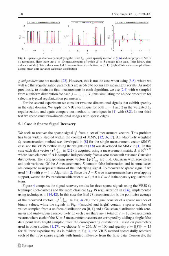
Fig. 4 Sparse signal recovery employing the usual �2,1 joint sparsity method in (2.6) and our proposed VBJS
�1 technique. Here there are J = 10 measurements of which K = 5 contain false data. (left) Binary data
values. (middle) Data values sampled from a uniform distribution on [0, 1]. (right) Data values sampled from
a zero-mean unit-variance Gaussian distribution
g-subproblem are not needed [22]. However, this is not the case when using (3.8), where we
will see that regularization parameters are needed to obtain any meaningful results. As noted
previously, to obtain the first measurements in each algorithm, we use (2.4) with μ sampled
from a uniform distribution for each j = 1, . . . , J , thus simulating the ad-hoc procedure for
selecting typical regularization parameters.
For the second experiment we consider two one-dimensional signals that exhibit sparsity
in the edge domain. We apply the VBJS technique for both p = 1 and 2 in the weighted �p
regularization, and again compare our method to techniques in [1] with (3.8). In our third
test we reconstruct two-dimensional images with sparse edges.
5.1 Case 1: Sparse Signal Recovery
We seek to recover the sparse signal f from a set of measurment vectors. This problem
has been widely studied within the context of MMV, [12,16,17]. An adaptively weighted
�1 reconstruction method was developed in [8] for the single measurement vector (SMV)
case, and the VBJS method using the weights in (3.8) was developed for MMV in [1]. In this
case each data vector { y j }Jj=1 in (2.2) is acquired using a measurement matrix A ∈ R
M×N
where each element of A is sampled independently from a zero mean unit variance Gaussian
distribution. The corresponding noise vectors {η j }Jj=1 are i.i.d. Gaussian with zero mean
and unit variance. Of the J measurements, K contain false information and in some cases
are complete misrepresentations of the underlying signal. To recover the sparse signal f we
used (4.1) with p = 1 in Algorithm 2. Since the J − K true measurements have overlapping
support, we use the PA transform with order m = 0, that is L = I in the sparsity regularization
term.
Figure 4 compares the signal recovery results for three sparse signals using the VBJS �1
technique (dot-dashed) and the more classical �2,1 JS regularization in (2.6), implemented
using techniques in [14,42]. In this case the final JS reconstruction is the pointwise average
of the recovered vectors, { fj }J
j=1. In Fig. 4(left), the signal consists of a sparse number of
binary values, while the signals in Fig. 4(middle) and (right) contain a sparse number of
values sampled from a uniform distribution on [0, 1] and a Gaussian distribution with zero-
mean and unit-variance respectively. In each case there are a total of J = 10 measurements
vectors where each of the K = 5 measurement vectors are corrupted by adding a single false
data point with height sampled from the corresponding distribution. Based on parameters
used in other studies, [1,27], we choose N = 256, M = 100 and sparsity s = || f ||0 = 15
for all three experiments. As is evident in Fig. 4, the VBJS method successfully recovers
each of the three sparse signals with limited influence from the false data. Conversely, the
123

J Sci Comput (2019) 78:94–120 109
Table 1 Relative reconstruction errors (5.1) for the traditional �2,1 JS method and the VBJS method with
p = 1 using the weights defined in (3.6) and (3.8)
False data (%) Binary Uniform Gaussian
JS �2,1 (3.6) (3.8) JS �2,1 (3.6) (3.8) JS�2,1 (3.6) (3.8)
0 .0127 .0104 .0383 .0254 .0244 .0579 .0142 .0153 .0388
20 .1724 .0094 .0288 .1068 .0234 .0594 .1304 .0144 .0314
50 .2961 .0108 .0499 .2943 .0243 .0621 .1249 .0168 .0262
90 .1543 .0083 .0358 .3089 .0196 .0775 .1233 .0128 .0397
Fig. 5 Probability of successful recovery of the sparse (left) binary signal, (middle) uniform signal, and (right)
Gaussian signal with J = 10, 20 and 30 measurements, none of which contain false data. Recovery is deemed
a success if || g − f ||∞ ≤ 5 × 10⁻³, where g is the recovery vector and f is the true solution vector
classic �2,1 JS method is indeed influenced by the bad data. Similar behavior (not reported
here) can be observed for different choices of N , M J, K and s.
Table 1 displays the relative error,
E = || g − f ||2|| f ||2
, (5.1)
for the recovery vector g. In each case we use J = 10 measurements where K , the number of
false data measurements, is based on the given percentage in the first column. For consistent
comparison we use N = 256, M = 100 and sparsity s = || f ||0 = 20 in all cases. It is
evident that the VBJS �1 technique yields small error even as the percentage of false data
increases. Conversely, the traditional �2,1 JS method is more susceptible to false data. For
comparison we included results using the weights given in (3.8). We note that to handle the
noise and different jump heights in the problem, when using the weights in (3.8), we must
solve (3.4) by tuning the parameter μ to μ = .1. Regardless, it is evident that the weights
designed in (3.6) outperform the weights in (3.8) in all cases, and in the former case, no
additional parameter tuning is needed.
To further demonstrate the success of our method, at varying levels of sparsity for different
numbers of measurements and false data, we calculate the probability that the sparse signal
is successfully recovered. Similar analysis was done in [8,12,16,17,24,44]. Specifically, the
probability of recovery is calculated over 100 trials at the specified configuration (J , K , and
sparsity level) with N = 256, M = 100 and no additive noise. Recovery is deemed a success
if || g− f ||∞ ≤ 5×10⁻³, that is, when the VBJS method can successfully distinguish signals
larger than the resolution size, O( 1N
).
In Fig. 5 we see the recovery plots for each of the three signals considered with J = 10, 20
and 30 measurements, none of which contain false data. In this case, additional measure-
ments do not improve the already high recovery rates. However, in Fig. 6 we see that as
123

110 J Sci Comput (2019) 78:94–120
Fig. 6 The probability of recovery of the sparse signal with values sampled from a Gaussian distribution with
zero-mean and unit-variance for various combinations of J, K and || f ||0. Here N = 256 and M = 100. (left)
Binary sparse vectors, (middle) uniform sparse vectors and (right) Gaussian sparse vectors
the percentage of measurements that are false increases, it becomes more advantageous to
have more measurements. Across top row of Fig. 6 the percentage of false data increases to
50% while the number of measurements changes from J = 10, 20 to 30 for each type of
sparse vector (binary, uniform, and Gaussian). Across the bottom row of Fig. 6 the number of
measurements J = 20 remains fixed, while the percentage of false data included increases
from 20 to 50 to 90%. We see that when 50% of the measurements are false, the probability of
recovery remains high for large sparsity values. When the percentage of false data increases
to 90%, most probability of recovery values fall below .5.
5.2 Case 2: Reconstructing One Dimensional Piecewise Smooth Functions
We now consider the reconstruction of two piecewise smooth functions, given by
Example 1 Define f (x) on [−π, π] as
f (x) =
⎧
⎪
⎪
⎪
⎨
⎪
⎪
⎪
⎩
32, − 3π
4≤ x < −π
274
− x2
+ sin(
x − 14
)
, − π4
≤ x < π8
114
x − 5, 3π8
≤ x < 3π4
0, otherwise.
Example 2 Define f (x) on [−1, 1] as
f (x) =
⎧
⎪
⎨
⎪
⎩
cos(
π2
x)
, − 1 ≤ x < − 12
cos(
3π2
x)
, − 12
≤ x < 12
cos(
7π2
x)
, 12
≤ x ≤ 1
Each function exhibits sparsity in the jump function domain, that is f is not sparse, but
||[ f ]||0 = s, with s << N , and [ f ] = {[ f ](x j )}Nj=1 is the corresponding vector of edges.
We consider the proposed weights (3.6) and the weights given by (3.8) in [1] for the weighted
�p reconstructions (3.4) with p = 1 and 2.
123
J Sci Comput (2019) 78:94–120 111
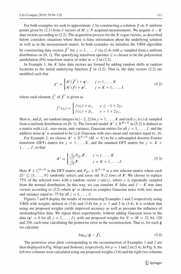
For both examples we seek to approximate f by constructing a solution f on N uniform
points given by (2.1) from J vectors of M ≤ N acquired measurements. We acquire J − K
data vectors according to (2.2). The acquisition process for the K rogue vectors, as described
below, considers situations where there is false information about the underlying solution
as well as in the measurement matrix. In both examples we initialize the VBJS algorithm
by constructing data vectors fj
for j = 1, . . . , J via (2.4) with μ sampled from a uniform
distribution on [0, 1]. The sparsifying transform operator L is chosen to be the polynomial
annihilation (PA) transform matrix of order m = 2 in (3.2).
In Example 1, the K false data vectors are formed by adding random shifts at random
locations to the initial underlying function f in (2.2). That is, the data vectors (2.2) are
modified such that
y j ={
A j ( fj) + η j , j = 1, . . . , K
A j ( f ) + η j , j = K + 1, . . . , J,(5.2)
where each element fj
i of fj
is given as
f j (xi ) ={
f (xi ) + α j , x ≤ −1 + 2γ j
f (xi ) + β j , x > 1 + 2γ j .
Here α j and β j are random integers in [− 2, 2] for j = 1, . . . , K and each γ j is i.i.d. sampled
from a uniform distribution on [0, 1]. The forward model A j ∈ RM×N in (5.2) is defined as
a matrix with i.i.d., zero-mean, unit-variance, Gaussian entries for all j = 1, . . . , J , and the
additive noise η j is assumed to be i.i.d. Gaussian with zero-mean and variance equal to .16.
For Example 2, we choose A j ∈ RN×N (M = N ) to be a subsampled discrete Fourier
transform (DFT) matrix for j = 1, . . . , K , and the standard DFT matrix for j = K +1, . . . , J , so that
A j ={
1√N
PΩ j F, j = 1, . . . , K
1√N
F, j = K + 1, . . . , J.(5.3)
Here F ∈ CN×N is the DFT matrix and PΩ j ∈ R
N×N is a row selector matrix where each
Ω j ⊆ {1, . . . , N } randomly selects and zeros out N/2 rows of F. We choose to replace
75% of the selected rows with a random vector γ sin(x), where γ is repeatedly sampled
from the normal distribution. In this way, we can simulate K false and J − K true data
vectors according to (2.2) where η j is chosen as complex Gaussian noise with zero mean
and variance equal to .75 for all j = 1, . . . , J .
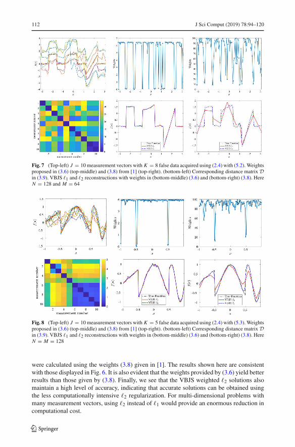
Figures 7 and 8 display the results of reconstructing Examples 1 and 2 respectively using
VBJS with weights defined in (3.6) and (3.8) for p = 1 and 2 in (3.4). It is evident that
using our proposed weights yields improved accuracy as well as prevents the influence of
misleading/false data. We repeat these experiments, without adding Gaussian noise to the
data (η j = 0 for all j = 1, . . . , J ), with our proposed weights for N = M = 32, 64, 128
and 256, each time calculating the pointwise error in the reconstruction. That is, for each g
we calculate
log10 | g − f |. (5.4)
The pointwise error plots corresponding to the reconstruction of Examples 1 and 2 are
then displayed in Fig. 9(top) and (bottom), respectively, for p = 1 and 2 in (3.4). In Fig. 9, the
left two columns were calculated using our proposed weights (3.6) and the right two columns
123
112 J Sci Comput (2019) 78:94–120
Fig. 7 (Top-left) J = 10 measurement vectors with K = 8 false data acquired using (2.4) with (5.2). Weights
proposed in (3.6) (top-middle) and (3.8) from [1] (top-right). (bottom-left) Corresponding distance matrix D
in (3.9). VBJS �1 and �2 reconstructions with weights in (bottom-middle) (3.6) and (bottom-right) (3.8). Here
N = 128 and M = 64
Fig. 8 (Top-left) J = 10 measurement vectors with K = 5 false data acquired using (2.4) with (5.3). Weights
proposed in (3.6) (top-middle) and (3.8) from [1] (top-right). (bottom-left) Corresponding distance matrix D
in (3.9). VBJS �1 and �2 reconstructions with weights in (bottom-middle) (3.6) and (bottom-right) (3.8). Here
N = M = 128
were calculated using the weights (3.8) given in [1]. The results shown here are consistent
with those displayed in Fig. 6. It is also evident that the weights provided by (3.6) yield better
results than those given by (3.8). Finally, we see that the VBJS weighted �2 solutions also
maintain a high level of accuracy, indicating that accurate solutions can be obtained using
the less computationally intensive �2 regularization. For multi-dimensional problems with
many measurement vectors, using �2 instead of �1 would provide an enormous reduction in
computational cost.
123

J Sci Comput (2019) 78:94–120 113
Fig. 9 The pointwise error of the VBJS reconstructions of (top) Example 1 and (bottom) Example 2 for
N = M = 32, 64, 128 and 256 with J = 20 measurements K = 4 of which are false with p = 1 (left,right-
middle) and p = 2 (left-middle,right). In (left, left-middle) we use the weights given in (3.6) and in (right,
right-middle) we use the weights given in (3.8)
Table 2 Relative reconstruction errors (5.1) for the VBJS method (3.4) with p = 1 and 2 using the weights
defined in (3.6) and (3.8)
SMV �1 (3.6) �2 (3.6) �1 (3.8) �2 (3.8)
Example 1 .0844 .0335 .0393 .4173 .1694
Example 2 .0692 .0536 .0716 .3142 .0959
Here N = M = 128
Table 3 Absolute error near a discontinuity for the VBJS method (3.4) with p = 1 and 2 using the weights
defined in (3.6) and (3.8)
SMV �1 (3.6) �2 (3.6) �1 (3.8) �2 (3.8)
Example 1 .1417 .0048 .0285 .3440 .4276
Example 2 .0131 .0206 .0132 .3738 .1325
In Example 1, x∗ = 1.23 and in Example 2, x∗ = −.55. Here N = M = 128
For further comparison, Table 2 displays the relative error (5.1) for each example, while
Table 3 measures the performance at a neighboring grid point to a jump discontinuity, given
by
| f (x∗) − g(x∗)|.
For the SMV approximation we choose y using (3.10), that is, we consider the best possible
solution. In each case we use J = 10 measurements where K = 5 vectors contain false
infromation. Observe that using the VBJS algorithm with the weights in (3.6) with either
�1 or �2 regularization yields better accuracy than the weights in (3.8), proposed in [1].
These results occur without any additional parameter tuning, which is required for both the
SMV and VBJS using (3.8). Our method also shows general improvement over the SMV
approximation, (2.4), which does not contain any false information.
123
114 J Sci Comput (2019) 78:94–120
5.3 Case 3: Reconstructing Two Dimensional Images
We now consider reconstructing two dimensional images using the VBJS approach. We note
that the original polynomial annihilation edge detection method constructed in [4] was, by
design, multi-dimensional. However, as was discussed in [3], for optimization algorithms
using �1 regularization, applying the PA transform dimension by dimension was both more
efficient and more accurate when on a uniform grid. Therefore, to calculate the weights
(3.6) in the two dimensional case, we first calculate the two dimensional edge map for each
j = 1, . . . , J as
Ej = L f
j + fjL
T .
The columns of each Ej , j = 1, . . . , J , are then stacked on top of each other to form
the matrix of J vectors of approximations of some sparse feature of the underlying image,
i.e. the two dimensional analogue of (3.2). Continuing as in one dimension, the weights
are now calculated according to (3.6) and then reshaped into a matrix W ∈ RN×N . The
non-zero entries wi, j correspond to the sparse regions of the image, while the entries are
approximately zero whenever an edge is assumed to be present. Observe that W is not sparse,
so the implementation methods developed in Sect. 4 is critical for numerical efficiency.
As in the one dimensional case, we consider two examples:
Example 3 Define f (x, y) on [−1, 1]2 as
f (x, y) =
⎧
⎪
⎨
⎪
⎩
15, |x |, |y| ≤ 14
20, |x |, |y| > 14,
√
x2 + y2 ≤ 34
10, else
Example 4 Define f (x, y) on [− 1, 1]2 as
f (x, y) =
⎧
⎨
⎩
10 cos(
3π2
√
x2 + y2)
,√
x2 + y2 ≤ 12
10 cos(
π2
√
x2 + y2)
,√
x2 + y2 > 12
We sample each function f : RN×N → R on a uniform grid as fi,l = f (xi , yl), where
xi = −1 + 2
N(i − 1), yl = −1 + 2
N(l − 1),
for each i, l = 1, . . . , N . In (2.2), A : RN×N → C
N×N is defined to be the normalized,
two dimensional discrete Fourier transform operator so that A∗ = A−1, and η j is zero mean
complex Gaussian noise with .5 variance for all j = 1, . . . , J . As in the one dimensional case
we use (2.4) to construct each fj. Because of the piecewise constant nature of Example 3
we apply the PA transform with order m = 1. Similarly, for Example 4 we use m = 2.
We note that it is possible to use m > 2, but in this case, because of the noise, the higher
order polynomial approximation leads to overfitting. For each data vector the regularization
parameter μ is sampled from a uniform distribution on [0, 10].Figure 10 displays the result of applying VBJS with �1 (middle-right) and �2 (right) to
Examples 3 and 4. For both examples we use J = 10 measurement vectors where K = 5
falsely represent the underlying function. (The corresponding measurement selection matri-
ces (3.9) are shown in Fig. 11(right).) Figure 10(middle-left) shows the the SMV results on
the measurement vector selected by (3.9) calculated using (2.4). It is evident in both exam-
ples that the VBJS technique with either p = 1 or 2 in (3.4) leads to improved visualization
123

J Sci Comput (2019) 78:94–120 115
Fig. 10 (Left) Weights calculated using (3.6), where the darker shades indicate wi, j ≈ 0. (middle-left)
Reconstruction of a single measurement vector using (3.9) and (2.4). (middle-right) VBJS with p = 1. (right)
VBJS with p = 2. (top) Example 3 reconstruction performed with PA transform of order m = 1 in (3.2).
(bottom) Example 4 reconstruction performed with PA transform of order m = 2 in (3.2)
Fig. 11 (Top) Results corresponding to Example 3. (bottom) results corresponding to Example 4. (left) Cross
sections (y = 0) of J = 10 measurement vectors with K = 5 false data representations. (middle) Cross
sections (y = 0) of VBJS reconstructions for p = 1 and 2 in (3.4) compared to the SMV constructed using
(2.4). (right) Data selection matrices D
over the standard SMV reconstruction, even when the standard SMV uses the “best” initial-
ization as determined by (3.9). This result is confirmed in Fig. 11, where we compare the
corresponding one-dimensional cross sections at y = 0.
6 Concluding Remarks
In this investigation we proposed a modification to the variance based joint sparsity technique
(VBJS), introduced in [1], in both the weighting vector and in the choice of reconstruction
123

116 J Sci Comput (2019) 78:94–120
vector. Our adaptation is especially critical when some data vectors contain false measure-
ments. We additionally proved that the ADMM algorithm could be successfully used for the
weighted �1 case, and moreover, that for our choice of weights in (3.6), no extra parameter
tuning is needed to achieve high accuracy and fast convergence. Hence our method is robust
and suitable to a wide range of problems. We also presented a corresponding gradient descent
method for the weighted �2 case.
Our numerical results demonstrate that the VBJS method with the weights designed in
(3.6) yields improved accuracy and robustness over the single measurement vector case, the
classical �2,1 JS method, and the original VBJS method proposed in [1]. By including an
optimal data vector selection step, we are able to obtain high accuracy and good sparse signal
recovery even when a subset of the given measurement data misrepresents the underlying
function. Furthermore, using the weighted �2 norm also yields good results and is much more
cost effective than the weighted �1 reconstructions.
In future investigations we will conduct a thorough convergence analysis of the VBJS
method, in particular to establish rigorous results for the weighted �2 case. We will also
parallelize our algorithm so that we may test it on synthetic aperture radar automatic target
recognition problems, where current algorithms fail when obstructions are added to (or taken
out of) imaging scenes. Because our method is non-parametric, autonomy will be maintained.
This framework also lends itself to data fusion problems, where measurements of a scene are
obtained through multiple imaging techniques and must be combined to yield optimal results.
Finally, the VBJS can potentially be used in numerical partial differential equation solvers,
in particular to develop predictor-corrector methods for equations that exhibit singularities
or for which shock discontinuities evolve.
A Proof of Lemma 1
Proof [Lemma 1] Following the technique described in [22] for the non-weighted, one-
dimensional case, let x ∈ RN×N and wi, j ≥ 0 for all i, j = 1, . . . , N . We drop the vec
notation for simplicity.
Define the objective function H : RN×N → R
N×N as
H(x) := ||x ||1,w − νT (y − x) + β
2||y − x ||22. (A.1)
To show H(x) is convex, we first observe that for α ∈ (0, 1) and p, q ∈ RN×N , we have
||y − αp − (1 − α)q||22 −(
α||y − p||22 + (1 − α)||y − q||22)
= (y − αp − (1 − α)q)T (y − αp − (1 − α)q)
−(
α(y − p)T (y − p) + (1 − α)(y − q)T (y − q)
)
= α(α − 1)
(
pT p − pT q − qT p + qT q)
= α(α − 1)||p − q||22≤ 0.
(A.2)
123

J Sci Comput (2019) 78:94–120 117
Applying (A.2) to H yields
H(αp + (1 − α)q) − (αH(p) + (1 − α)H(q))
= ||αp + (1 − α)q||1,w − νT (y − (αp + (1 − α)q)) + β
2||y − (αp + (1 − α)q)||22
− α||p||1,w − (1 − α)||q||1,w + ανT (y − p) + (1 − α)νT (y − q)
− βα
2||y − p||22 − β(1 − α)
2||y − q||22
≤ β
2||y − (αp + (1 − α)q)||22 − βα
2||y − p||22 − β(1 − α)
2||y − q||22
= β
2α(α − 1)||p − q||22
≤ 0.
(A.3)
Therefore H is convex. For p �= q , H is strictly/strongly convex and thus coercive [6,7,28].
Hence there exists at least one solution x of (4.6), [38].
The subdifferential of f (x) = ||x ||1,w is given element-wise as
(∂x f (x))i, j ={
sign(xi, j )wi, j , xi, j �= 0{
h; |h| ≤ wi, j , h ∈ R}
, otherwise,(A.4)
where the origin is required to be included according to the optimality condition for convex
problems. According to (A.4), to minimize (A.1), each component xi, j , i, j = 1, . . . , N ,
must satisfy
{
sign(xi, j )wi, j + β(xi, j − yi, j ) + νi, j = 0, xi, j �= 0
|vi, j − βyi, j | ≤ wi, j , otherwise.(A.5)
If xi, j �= 0, (A.5) yields
wi, j
βsign(xi, j ) + xi, j = yi, j − νi, j
β. (A.6)
Since wi, j/β > 0, (A.6) implies
wi, j
β+ |xi, j | =
∣
∣
∣
∣
yi, j − νi, j
β
∣
∣
∣
∣
. (A.7)
Combining (A.6) and (A.7) gives
sign(xi, j ) = sign(xi, j )|xi, j | + sign(xi, j )wi, j/β
|xi, j | + wi, j/β= xi, j + sign(xi, j )wi, j/β
|xi, j | + wi, j/β
= yi, j − νi, j/β
|yi, j − νi, j/β| = sign
(
yi, j − νi, j
β
) (A.8)
Thus, for xi, j �= 0, we have
xi, j = |xi, j |sign(xi, j ) =(
|yi, j − νi, j
β| − wi, j
β
)
sign
(
yi, j − νi, j
β
)
, (A.9)
where we have used (A.7) and (A.8) in the result.
123

118 J Sci Comput (2019) 78:94–120
Conversely, we now show that xi, j = 0 if and only if
∣
∣
∣
∣
yi, j − νi, j
β
∣
∣
∣
∣
≤ wi, j
β. (A.10)
First assume that xi, j = 0. Then (A.10) follows from (A.5) since β > 0.
Now assume (A.10) holds for some xi, j �= 0. By (A.5), xi, j satisfies (A.7). Hence
∣
∣xi, j
∣
∣ =∣
∣
∣
∣
yi, j − νi, j
β
∣
∣
∣
∣
− wi, j
β≤ 0
which only holds for xi, j = 0. Hence by contradiction, xi, j = 0. Combining (A.10) with
(A.9) yields
xi, j = max
{
|yi, j − νi, j
β| − wi, j
β, 0
}
sign
(
yi, j − νi, j
β
)
.
which is equivalent to (4.7) in matrix form.
References
1. Adcock, B., Gelb, A., Song, G., Sui, Y.: Joint sparse recovery based on variances. SIAM J. Sci. Comput.
(submitted)
2. Ao, D., Wang, R., Hu, C., Li, Y.: A sparse SAR imaging method based on multiple measurement vectors
model. Remote Sens. 9(3), 297 (2017)
3. Archibald, R., Gelb, A., Platte, R.B.: Image reconstruction from undersampled Fourier data using the
polynomial annihilation transform. J. Sci. Comput. 67(2), 432–452 (2016)
4. Archibald, R., Gelb, A., Yoon, J.: Polynomial fitting for edge detection in irregularly sampled signals and
images. SIAM J. Numer. Anal. 43(1), 259–279 (2005)
5. Barzilai, J., Borwein, J.M.: Two-point step size gradient methods. IMA J. Numer. Anal. 8(1), 141–148
(1988)
6. Bauschke, H.H., Combettes, P.L.: Convex Analysis and Monotone Operator Theory in Hilbert Spaces,
vol. 408. Springer, New York (2011)
7. Beck, A.: Introduction to Nonlinear Optimization: Theory, Algorithms, and Applications with MATLAB.
SIAM (2014)
8. Candes, E.J., Wakin, M.B., Boyd, S.P.: Enhancing sparsity by reweighted �1 minimization. J. Fourier
Anal. Appl. 14(5), 877–905 (2008)
9. Chan, T., Marquina, A., Mulet, P.: High-order total variation-based image restoration. SIAM J. Sci.
Comput. 22(2), 503–516 (2000)
10. Chartrand, R., Yin, W.: Iteratively reweighted algorithms for compressive sensing. In: IEEE International
Conference on Acoustics, Speech and Signal Processing, 2008. ICASSP 2008. pp. 3869–3872. IEEE,
(2008)
11. Chen, J., Huo, X.: Theoretical results on sparse representations of multiple-measurement vectors. IEEE
Trans. Signal Process. 54(12), 4634–4643 (2006)
12. Cotter, S.F., Rao, B.D., Engan, K., Kreutz-Delgado, K.: Sparse solutions to linear inverse problems with
multiple measurement vectors. IEEE Trans. Signal Process. 53(7), 2477–2488 (2005)
13. Daubechies, I., DeVore, R., Fornasier, M., Güntürk, C.S.: Iteratively reweighted least squares minimization
for sparse recovery. Commun. Pure Appl. Math. 63(1), 1–38 (2010)
14. Deng, W., Yin, W., Zhang, Y.: Group sparse optimization by alternating direction method. In: Technical
Report. Rice University, Houston, TX, Department of Computationa and Applied Mathematics, (2012)
15. Denker, D., Gelb, A.: Edge detection of piecewise smooth functions from undersampled Fourier data
using variance signatures. SIAM J. Sci. Comput. 39(2), A559–A592 (2017)
16. Eldar, Y.C., Mishali, M.: Robust recovery of signals from a structured union of subspaces. IEEE Trans.
Inf. Theory 55(11), 5302–5316 (2009)
17. Eldar, Y.C., Rauhut, H.: Average case analysis of multichannel sparse recovery using convex relaxation.
IEEE Trans. Inf. Theory 56(1), 505–519 (2010)
123

J Sci Comput (2019) 78:94–120 119
18. Fu, W., Li, S., Fang, L., Kang, X., Benediktsson, J.A.: Hyperspectral image classification via shape-
adaptive joint sparse representation. IEEE J. Sel. Top. Appl. Earth Obs. Remote Sens. 9(2), 556–567
(2016)
19. Glowinski, R., Le Tallec, P.: Augmented Lagrangian and operator-splitting methods in nonlinear mechan-
ics. Studies in applied and numerical mathematics, pp. 45–121. SIAM (1989)
20. Keydel, E.R., Lee, S.W., Moore, J.T.: MSTAR extended operating conditions: a tutorial. In:
Aerospace/Defense Sensing and Controls, International Society for Optics and Photonics pp. 228–242
(1996)
21. Leviatan, D., Temlyakov, V.N.: Simultaneous approximation by greedy algorithms. Adv. Comput. Math.
25(1), 73–90 (2006)
22. Li, C.: An efficient algorithm for total variation regularization with applications to the single pixel camera
and compressive sensing. In: Ph.D. Thesis, Citeseer (2009)
23. Liu, L., Esmalifalak, M., Ding, Q., Emesih, V.A., Han, Z.: Detecting false data injection attacks on power
grid by sparse optimization. IEEE Trans. Smart Grid 5(2), 612–621 (2014)
24. Liu, Q.Y., Zhang, Q., Gu, F.F., Chen, Y.C., Kang, L., Qu, X.Y.: Downward-looking linear array 3D SAR
imaging based on multiple measurement vectors model and continuous compressive sensing. J. Sens.
2017, 1–12 (2017)
25. Liu, Y., Ma, J., Fan, Y., Liang, Z.: Adaptive-weighted total variation minimization for sparse data toward
low-dose X-ray computed tomography image reconstruction. Phys. Med. Biol. 57(23), 7923 (2012)
26. Mishali, M., Eldar, Y.C.: Reduce and boost: Recovering arbitrary sets of jointly sparse vectors. IEEE
Trans. Signal Process. 56(10), 4692–4702 (2008)
27. Monajemi, H., Jafarpour, S., Gavish, M., Donoho, D.L., Ambikasaran, S., Bacallado, S., Bharadia, D.,
Chen, Y., Choi, Y., Chowdhury, M., et al.: Deterministic matrices matching the compressed sensing phase
transitions of Gaussian random matrices. Proc. Nat. Acad. Sci. 110(4), 1181–1186 (2013)
28. Niculescu, C., Persson, L.E.: Convex functions and their applications: a contemporary approach. Springer,
New York (2006)
29. Parikh, N., Boyd, S., et al.: Proximal algorithms. Found. Trends Optim. 1(3), 127–239 (2014)
30. Sanders, T., Gelb, A., Platte, R.B.: Composite SAR imaging using sequential joint sparsity. J. Comput.
Phys. 338, 357–370 (2017)
31. Singh, A., Dandapat, S.: Weighted mixed-norm minimization based joint compressed sensing recovery
of multi-channel electrocardiogram signals. Comput. Electr. Eng. 53, 203–218 (2016)
32. Steffens, C., Pesavento, M., Pfetsch, M.E.: A compact formulation for the l21 mixed-norm minimization
problem. In: IEEE International Conference on Acoustics, Speech and Signal Processing (ICASSP), 2017,
pp. 4730–4734. IEEE, (2017)
33. Tropp, J.A.: Algorithms for simultaneous sparse approximation. Part II: convex relaxation. Signal Process.
86(3), 589–602 (2006)
34. Tropp, J.A., Gilbert, A.C., Strauss, M.J.: Simultaneous sparse approximation via greedy pursuit. In:
IEEE International Conference and Proceedings on Acoustics, Speech, and Signal Processing, 2005.
(ICASSP’05), vol. 5, pp. v–721. IEEE (2005)
35. Tropp, J.A., Gilbert, A.C., Strauss, M.J.: Algorithms for simultaneous sparse approximation. Part I: greedy
pursuit. Signal Process. 86(3), 572–588 (2006)
36. Wang, Y., Yang, J., Yin, W., Zhang, Y.: A new alternating minimization algorithm for total variation image
reconstruction. SIAM J. Imaging Sci. 1(3), 248–272 (2008)
37. Wipf, D.P., Rao, B.D.: An empirical bayesian strategy for solving the simultaneous sparse approximation
problem. IEEE Trans. Signal Process. 55(7), 3704–3716 (2007)
38. Wright, S., Nocedal, J.: Numerical optimization. Science 35, 67–68 (1999)
39. Xie, W., Deng, Y., Wang, K., Yang, X., Luo, Q.: Reweighted l1 regularization for restraining artifacts in
fmt reconstruction images with limited measurements. Opt. Lett. 39(14), 4148–4151 (2014)
40. Yang, Z., Xie, L.: Enhancing sparsity and resolution via reweighted atomic norm minimization. IEEE
Trans. Signal Process. 64(4), 995–1006 (2016)
41. Ye, F., Luo, H., Lu, S., Zhang, L.: Statistical en-route filtering of injected false data in sensor networks.
IEEE J. Sel. Areas Commun. 23(4), 839–850 (2005)
42. Zhang, Y.: Users guide for YALL1: your algorithms for l1 optimization. In: Technique Report, pp. 09–17
(2009)
43. Zhao, B., Fei-Fei, L., Xing, E.P.: Online detection of unusual events in videos via dynamic sparse coding.
In: 2011 IEEE Conference on Computer Vision and Pattern Recognition (CVPR), pp. 3313–3320. IEEE
(2011)
44. Zheng, C., Li, G., Liu, Y., Wang, X.: Subspace weighted l21 minimization for sparse signal recovery.
EURASIP J. Adv. Signal Process. 2012(1), 98 (2012)
123

120 J Sci Comput (2019) 78:94–120
45. Zhou, F., Wu, R., Xing, M., Bao, Z.: Approach for single channel SAR ground moving target imaging
and motion parameter estimation. IET Radar Sonar Navig. 1(1), 59–66 (2007)
123