reduction algorithms for the cryptanalysis of lattice based
TRANSCRIPT
REDUCTION ALGORITHMS FOR THECRYPTANALYSIS OF LATTICE BASEDASYMMETRICAL CRYPTOSYSTEMS
A Thesis Submitted tothe Graduate School of Engineering and Sciences of
Izmir Institute of Technologyin Partial Fulfillment of the Requirements for the Degree of
MASTER OF SCIENCE
in Computer Software
byMutlu BEYAZIT
August 2008IZMIR

We approve the thesis of Mutlu BEYAZIT
Assoc. Prof. Dr. Ahmet KOLTUKSUZSupervisor
Asst. Prof. Dr. Gokhan DALKILICCommittee Member
Dr. Serap ATAYCommittee Member
13 August 2008
Prof. Dr. Sıtkı AYTAC Prof. Dr. Hasan BOKEHead of the Computer Engineering Dean of the Graduate School ofDepartment Engineering and Sciences

ACKNOWLEDGEMENTS
To begin with, I would like to thank Dr. Ahmet Koltuksuz for providing me with
the opportunity to perform such a study.
Furthermore, I would like to thank my colleague Selma Tekir for pushing me
forward to complete my thesis and her endurance.
I would also like to thank my former roommate Ali Mersin. If he were here, this
thesis would not be finished (:D).
The (other) IS3 Lab. members, Burcu Kulahcıoglu, Murat Ozkan, Sevgi Uslu,
Evren Akalp, Huseyin Hısıl and Dr. Serap Atay, deserves my sincere thanks, too. It is a
pleasure to work with them.
I would also like to thank my fellow research assistants, Deniz Cokuslu, Fatih
Tekbacak and Orhan Dagdeviren for providing me with the latex templates.
Finally, I would like to thank my parents, Zahide and Yıldırım Beyazıt, my
brother, Kutlu Beyazıt, and my girlfriend, Esra Aycan, for their consideration and un-
derstanding.

ABSTRACT
REDUCTION ALGORITHMS FOR THE CRYPTANALYSIS OFLATTICE BASED ASYMMETRICAL CRYPTOSYSTEMS
The theory of lattices has attracted a great deal of attention in cryptology in re-
cent years. Several cryptosystems are constructed based on the hardness of the lattice
problems such as the shortest vector problem and the closest vector problem. The aim
of this thesis is to study the most commonly used lattice basis reduction algorithms,
namely Lenstra Lenstra Lovasz (LLL) and Block Kolmogorov Zolotarev (BKZ) algo-
rithms, which are utilized to approximately solve the mentioned lattice based problems.
Furthermore, the most popular variants of these algorithms in practice are evaluated ex-
perimentally by varying the common reduction parameter delta in order to propose some
practical assessments about the effect of this parameter on the process of basis reduction.
These kind of practical assessments are believed to have non-negligible impact on the
theory of lattice reduction, and so the cryptanalysis of lattice cryptosystems, due to the
fact that the contemporary nature of the reduction process is mainly controlled by the
heuristics.
iv

OZET
KAFES TABANLI ASIMETRIK KRIPTOSISTEMLERINKRIPTANALIZI ICIN INDIRGEME ALGORITMALARI
Son yıllarda, kafes teorisi kriptolojide buyuk ilgi gormektedir. En kısa vektor
problemi ve en yakın vektor problemi gibi kafes tabanlı problemlerin zorluguna daya-
narak bir cok kriptosistem insa edilmistir. Bu tezin amacı bahsedilen kafes tabanlı prob-
lemleri yaklasık olarak cozmek amacıyla en sık kullanılan kafes tabanı indirgeme algo-
ritmalarından Lenstra Lenstra Lovasz (LLL) ve Block Kolmogorov Zolotarev (BKZ)
algoritmalarının incelenmesidir. Bununla beraber, bu algoritmaların uygulamadaki
en yaygın degiskelerinde ortak delta indirgeme parametresi degistirilerek bu parame-
trenin indirgeme surecindeki etkisi deneysel olarak incelenmekte ve taban indirgeme
islemini ilgilendiren uygulama temelli degerlendirmeler ortaya konmaktadır. Gunumuz
indirgeme isleminin dogasının agırlıklı olarak bulussal yontemlerce kontrol edilmesi
nedeniyle bu tip uygulama temelli degerlendirmelerin kafes indirgeme teorisinde, ve
buna baglı olarak kafes kriptosistemlerinin kriptanalizinde, ihmal edilemeyecek etkileri
olduguna inanılmaktadır.
v

TABLE OF CONTENTS
LIST OF FIGURES . . . . . . . . . . . . . . . . . . . . . . . . . . . . . . . . x
CHAPTER 1 . INTRODUCTION . . . . . . . . . . . . . . . . . . . . . . . . . 1
CHAPTER 2 . BACKGROUND . . . . . . . . . . . . . . . . . . . . . . . . . . 5
2.1. Lattice and Basis . . . . . . . . . . . . . . . . . . . . . . . . 5
2.2. Determinant . . . . . . . . . . . . . . . . . . . . . . . . . . . 6
2.3. Successive Minima and Hermite’s Constant . . . . . . . . . . 7
2.4. Important Theorems . . . . . . . . . . . . . . . . . . . . . . 8
2.5. Referential . . . . . . . . . . . . . . . . . . . . . . . . . . . 10
CHAPTER 3 . LATTICE PROBLEMS . . . . . . . . . . . . . . . . . . . . . . 11
3.1. SVP and CVP . . . . . . . . . . . . . . . . . . . . . . . . . . 11
3.2. Summary of Complexity Results . . . . . . . . . . . . . . . . 13
3.2.1. SVP Hardness . . . . . . . . . . . . . . . . . . . . . . . 13
3.2.2. CVP Hardness . . . . . . . . . . . . . . . . . . . . . . . 15
3.2.3. SVP and CVP Non-hardness . . . . . . . . . . . . . . . . 15
3.2.4. Results in l∞ Norm . . . . . . . . . . . . . . . . . . . . . 16
3.2.5. SVP-CVP Reductions . . . . . . . . . . . . . . . . . . . 17
3.3. Summary of Algorithmic Results . . . . . . . . . . . . . . . . 17
3.3.1. Approximating SVP . . . . . . . . . . . . . . . . . . . . 18
3.3.2. Solving SVP . . . . . . . . . . . . . . . . . . . . . . . . 20
3.3.3. Approximating CVP . . . . . . . . . . . . . . . . . . . . 20
3.3.4. Solving CVP . . . . . . . . . . . . . . . . . . . . . . . . 21
3.4. Basis Reduction and Other Lattice Problems . . . . . . . . . . 22
3.5. Referential . . . . . . . . . . . . . . . . . . . . . . . . . . . 23
CHAPTER 4 . LENSTRA LENSTRA LOVASZ REDUCTION . . . . . . . . . 24
4.1. LLL Reduced Basis . . . . . . . . . . . . . . . . . . . . . . . 24
4.2. LLL Basis Reduction Algorithm . . . . . . . . . . . . . . . . 25
vi
4.3. The Overview of Analysis . . . . . . . . . . . . . . . . . . . 28
4.3.1. Note on the Correctness . . . . . . . . . . . . . . . . . . 28
4.3.2. Note on the Running Time . . . . . . . . . . . . . . . . . 28
4.3.3. Note on the Approximation Factor . . . . . . . . . . . . . 30
4.4. LLL Basis Reduction Algorithm Rewritten . . . . . . . . . . 30
4.5. LLL Variants . . . . . . . . . . . . . . . . . . . . . . . . . . 32
4.5.1. LLL with Floating Point Arithmetic . . . . . . . . . . . . 32
4.5.2. Deep Insertions . . . . . . . . . . . . . . . . . . . . . . . 36
4.5.3. Segment LLL . . . . . . . . . . . . . . . . . . . . . . . . 36
4.5.4. Other Variants . . . . . . . . . . . . . . . . . . . . . . . 38
4.6. Brief Notes . . . . . . . . . . . . . . . . . . . . . . . . . . . 39
4.6.1. The importance of LLL . . . . . . . . . . . . . . . . . . 39
4.6.2. Generalized Lattice Basis Reduction Algorithm . . . . . . 39
4.6.3. Optimal and Average Case LLL . . . . . . . . . . . . . . 39
4.6.4. Parallel LLL . . . . . . . . . . . . . . . . . . . . . . . . 40
4.7. Referential . . . . . . . . . . . . . . . . . . . . . . . . . . . 40
CHAPTER 5 . BLOCK KORKINE ZOLOTAREV REDUCTION . . . . . . . . 41
5.1. HKZ, k - and Block 2k - Reduced Bases . . . . . . . . . . . . 41
5.2. Semi k - and Semi Block 2k - Reduced Bases . . . . . . . . . 43
5.3. Semi k-Reduction and Semi Block 2k-Reduction Algorithms . 46
5.4. Blockwise Lattice Basis Reduction Variants . . . . . . . . . . 50
5.4.1. BKZ Variants . . . . . . . . . . . . . . . . . . . . . . . . 50
5.4.2. Primal/Dual Segment Reduction . . . . . . . . . . . . . . 51
5.4.3. 2k-Block Rankin Reduction and Transference Reduction . 52
5.4.4. Slide Reduction . . . . . . . . . . . . . . . . . . . . . . . 52
5.5. Brief Notes . . . . . . . . . . . . . . . . . . . . . . . . . . . 53
5.5.1. Generalized Blockwise Lattice Basis Reduction . . . . . . 53
5.5.2. Improvement on the Nearest Plane Algorithm . . . . . . . 53
5.5.3. Parallel Block Reduction Algorithm . . . . . . . . . . . . 53
5.6. Referential . . . . . . . . . . . . . . . . . . . . . . . . . . . 53
vii

CHAPTER 6 . LINKING CRYPTANALYSIS . . . . . . . . . . . . . . . . . . 55
6.1. The Role of the Good Bases . . . . . . . . . . . . . . . . . . 55
6.1.1. Good Bases . . . . . . . . . . . . . . . . . . . . . . . . . 55
6.1.2. Good Bases and Lattice Problems . . . . . . . . . . . . . 56
6.2. A General Trapdoor Outline . . . . . . . . . . . . . . . . . . 58
6.3. Important Heuristics in Practice . . . . . . . . . . . . . . . . 59
6.3.1. Gaussian Heuristic . . . . . . . . . . . . . . . . . . . . . 59
6.3.2. Kannan’s Embedding Heuristic . . . . . . . . . . . . . . 60
6.4. Cryptanalytic Considerations and Lattice Attacks . . . . . . . 61
6.4.1. Brief Considerations . . . . . . . . . . . . . . . . . . . . 61
6.4.2. Lattice Attacks . . . . . . . . . . . . . . . . . . . . . . . 62
6.4.2.1. Lattice Attacks on the Private Key . . . . . . . . . 62
6.4.2.2. Lattice Attacks on the Message . . . . . . . . . . . 63
6.4.2.3. Lattice Attacks on a Spurious Key . . . . . . . . . . 64
6.4.2.4. An Example of Exploiting the Lattice Structure . . 64
6.5. Referential . . . . . . . . . . . . . . . . . . . . . . . . . . . 64
CHAPTER 7 . AN EVALUATION FOR EXPERIMENTS . . . . . . . . . . . . 66
7.1. Importance of the Practical Assessments . . . . . . . . . . . . 66
7.2. Preliminary Remarks . . . . . . . . . . . . . . . . . . . . . . 67
7.3. Experimental Details . . . . . . . . . . . . . . . . . . . . . . 69
CHAPTER 8 . CONCLUSION . . . . . . . . . . . . . . . . . . . . . . . . . . 71
8.1. Observations and Results . . . . . . . . . . . . . . . . . . . . 71
8.1.1. LLL XD . . . . . . . . . . . . . . . . . . . . . . . . . . 71
8.1.2. LLL XD DEEP . . . . . . . . . . . . . . . . . . . . . . 72
8.1.3. BKZ XD . . . . . . . . . . . . . . . . . . . . . . . . . . 74
8.1.4. A Short Comparison . . . . . . . . . . . . . . . . . . . . 76
8.2. Future Studies . . . . . . . . . . . . . . . . . . . . . . . . . . 77
REFERENCES . . . . . . . . . . . . . . . . . . . . . . . . . . . . . . . . . . . 79
APPENDICES
viii

APPENDIX A. LLL XD GRAPHS . . . . . . . . . . . . . . . . . . . . . . . . 92
APPENDIX B. LLL XD DEEP GRAPHS . . . . . . . . . . . . . . . . . . . . 94
APPENDIX C. BKZ XD GRAPHS . . . . . . . . . . . . . . . . . . . . . . . . 106
APPENDIX D. COMPARISON GRAPHS . . . . . . . . . . . . . . . . . . . . 118
ix

LIST OF FIGURES
Figure Page
Figure 4.1. LLL Lattice Basis Reduction Algorithm. . . . . . . . . . . . . . . 27
Figure 4.2. LLL Lattice Basis Reduction Algorithm (2). . . . . . . . . . . . . . 31
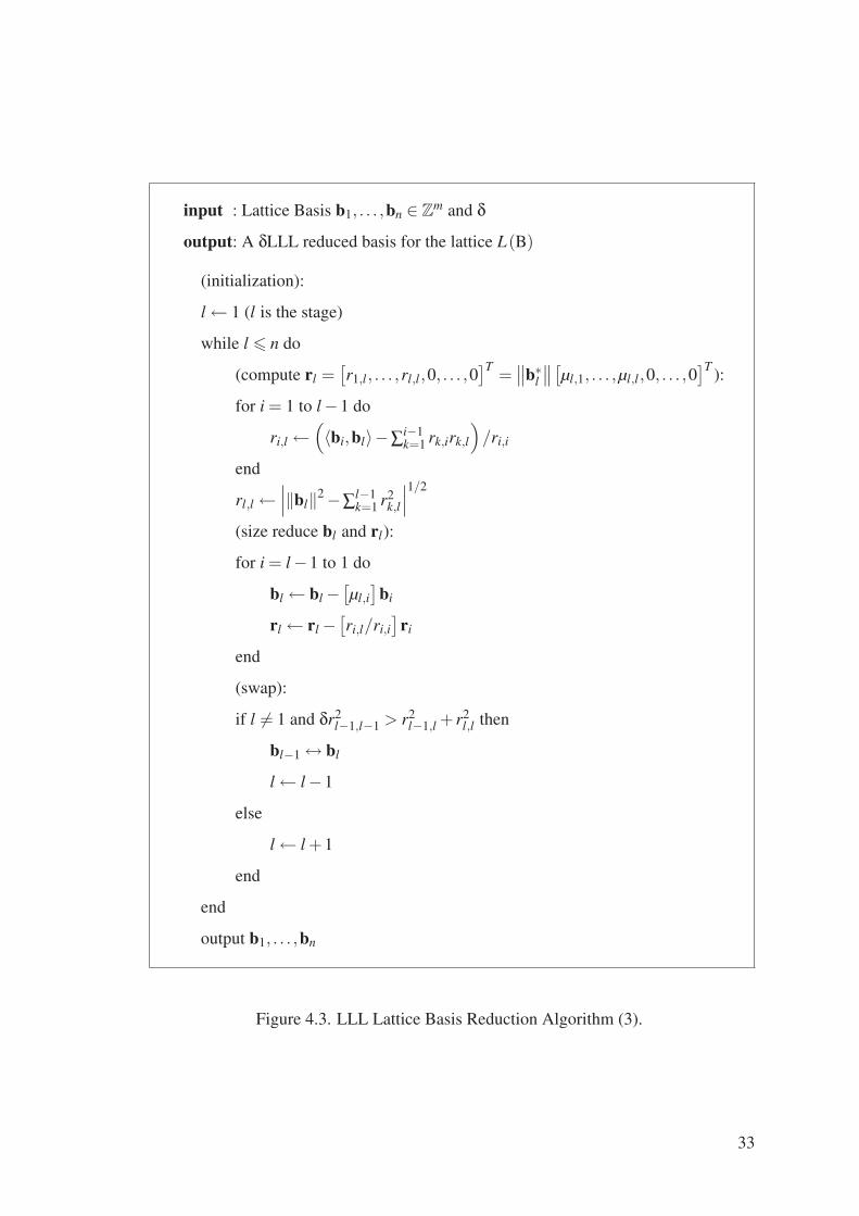
Figure 4.3. LLL Lattice Basis Reduction Algorithm (3). . . . . . . . . . . . . . 33
Figure 5.1. Semi k-Reduction Algorithm. . . . . . . . . . . . . . . . . . . . . 47
Figure 5.2. Semi Block 2k-Reduction Algorithm. . . . . . . . . . . . . . . . . 48
Figure 6.1. Good and Bad Bases. . . . . . . . . . . . . . . . . . . . . . . . . . 57
Figure 6.2. Translated Fundamental Parallelepipeds. . . . . . . . . . . . . . . . 57
Figure A.1. Running times of LLL XD. . . . . . . . . . . . . . . . . . . . . . . 92
Figure A.2. Approximation factor constants of LLL XD. . . . . . . . . . . . . . 93
Figure B.1. Running times of LLL XD DEEP in n (1). . . . . . . . . . . . . . . 94
Figure B.2. Running times of LLL XD DEEP in n (2). . . . . . . . . . . . . . . 95
Figure B.3. Running times of LLL XD DEEP in deep (1). . . . . . . . . . . . . 96
Figure B.4. Running times of LLL XD DEEP in deep (2). . . . . . . . . . . . . 97
Figure B.5. Running times of LLL XD DEEP in delta (1). . . . . . . . . . . . . 98
Figure B.6. Running times of LLL XD DEEP in delta (2). . . . . . . . . . . . . 99
Figure B.7. Approximation factor constants of LLL XD DEEP in n (1). . . . . . 100
Figure B.8. Approximation factor constants of LLL XD DEEP in n (2). . . . . . 101
Figure B.9. Approximation factor constants of LLL XD DEEP in deep (1). . . . 102
Figure B.10. Approximation factor constants of LLL XD DEEP in deep (2). . . . 103
Figure B.11. Approximation factor constants of LLL XD DEEP in delta (1). . . . 104
Figure B.12. Approximation factor constants of LLL XD DEEP in delta (2). . . . 105
Figure C.1. Running times of BKZ XD in n (1). . . . . . . . . . . . . . . . . . 106
Figure C.2. Running times of BKZ XD in n (2). . . . . . . . . . . . . . . . . . 107
Figure C.3. Running times of BKZ XD in blocksize (1). . . . . . . . . . . . . . 108
Figure C.4. Running times of BKZ XD in blocksize (2). . . . . . . . . . . . . . 109
Figure C.5. Running times of BKZ XD in delta (1). . . . . . . . . . . . . . . . 110
Figure C.6. Running times of BKZ XD in delta (2). . . . . . . . . . . . . . . . 111
Figure C.7. Approximation factor constants of BKZ XD in n (1). . . . . . . . . 112
Figure C.8. Approximation factor constants of BKZ XD in n (2). . . . . . . . . 113
x

Figure C.9. Approximation factor constants of BKZ XD in blocksize (1). . . . . 114
Figure C.10. Approximation factor constants of BKZ XD in blocksize (2). . . . . 115
Figure C.11. Approximation factor constants of BKZ XD in delta (1). . . . . . . 116
Figure C.12. Approximation factor constants of BKZ XD in delta (2). . . . . . . 117
Figure D.1. Comparison of running times. . . . . . . . . . . . . . . . . . . . . . 118
Figure D.2. Comparison of approximation factor constants. . . . . . . . . . . . . 119
xi

CHAPTER 1
INTRODUCTION
Lattices are constructions of geometry which can be described as the set of inter-
section points of an infinite regular grid. Though the simplicity in their construction, lat-
tices hide a rich complex structure which has attracted the interests of many mathemati-
cians over the last two centuries. In the meantime, they have found plenty of applications
in several branches of mathematics, especially in computer science. Their importance in
cryptology is firstly noted with the knapsack based cryptosystems. Invention of the basis
reduction algorithms and the breakthrough results of Ajtai on the hard problems over
lattices triggered numerous researches on the theory of lattices, more specifically on the
hard lattice problems and the lattice basis reduction algorithms. The aim of this study is
to explore the particular lattice problems and their use in cryptology with a cryptanalytic
perspective considering the practical algorithms to solve these problems.
The lattices are the source of many interesting computationally hard problems.
Two such problems are the shortest vector and the closest vector problem. The shortest
vector problem is by far the most popular lattice based problem and has many variations.
This problem stems from the fact that every lattice has a non-zero shortest vector and the
problem of finding such a vector is NP-hard. The impracticality of solving the shortest
vector problem in its exact form leads to the emergence of approximate versions related
to the problem. On the other hand, the closest vector problem is another important
problem in the theory of lattices. It includes finding a lattice vector which is among the
closest lattice vectors to an arbitrary target vector, or point, in the space. As in the case
of the shortest vector problem, the closest vector problem is also NP-hard and has many
variants.
The algorithms to solve the shortest vector problem can be classified as the exact
algorithms and the approximate algorithms. The main exact algorithms are the HKZ
(Hermite Korkine Zolotarev) reduction algorithms, (Kannan 1987b) and the (random-
ized) sieve algorithms, (Ajtai, et al. 2001). Whereas, the approximate algorithms are
primarily the LLL (Lenstra Lenstra Lovasz), (Lenstra, et al. 1982), algorithms and the
1

BKZ (Block Korkine Zolotarev) algorithms, (Schnorr 1987). In practice, the exact al-
gorithms are only practical in relatively low dimensions. Therefore, the approximation
algorithms attract comparatively more interest. An interesting point on the approxima-
tion algorithms and on some of the exact algorithms is that, in general, they do more
than just solving the approximate shortest vector problem, they produce a solution to the
lattice basis reduction problem. Basically, they output a shorter and more orthogonal
basis with particular properties, and this basis is deemed to be good in a practical point
of view, because it can be used to (approximately) solve different lattice based problems.
Another important point is that, all exact algorithms applies an approximation algorithm
for preprocessing and the approximation algorithms usually make use of the exact al-
gorithms by accessing them in low dimensions or relaxing their reduction conditions to
achieve a better performance.
It is also possible to group the algorithms to solve the closest vector problem
in two categories. The solution to the exact closest vector problem is mainly given by
the algorithms presented in (Kannan 1987b, Blomer 2000, Klein 2000, Agrell, et al.
2002). The approximation to the closest vector problem is performed in a roundabout
manner. The general approach is to use a reduction from the closest vector problem to
an instance of the (approximate) shortest vector problem together with an algorithm to
solve the reduced instance. This is a factor increasing the importance of the concept of
the lattice basis reduction. To name some of them, the approximation algorithms can be
found in (Babai 1986, Ajtai, et al. 2001, Blomer and Naewe 2007).
In this study, not all the algorithms to solve the referred lattice problems are
mentioned but instead the basis reduction algorithms which carry relatively greater im-
portance in the cryptanalysis of the lattice based public key cryptosystems are taken
under the consideration. For this reason, the following algorithmics and related concepts
are left out: the low dimensional reduction algorithms of Lagrange and Gauss , the al-
gorithms of Hermite , and Korkine and Zolotarev , the HKZ reduction algorithms (Kan-
nan 1983, 1987b, Helfrich 1985, Hanrot and Stehle 2007, 2008), the sieve algorithms
(Ajtai, et al. 2001, Schnorr 2001, Nguyen and Vidick 2008), the sampling algorithms
(Ajtai, et al. 2002, Schnorr 2003, Ludwig 2005, Buchmann and Ludwig 2006, Blomer
and Naewe 2007) and the closest vector algorithms (Kannan 1983, Babai 1986, Kannan
1987b, Schnorr 1996, Blomer 2000, Klein 2000, Ajtai, et al. 2001, Agrell, et al. 2002,
2
Blomer and Naewe 2007). Consequently, the LLL and the BKZ lattice basis reduction
algorithms are focused upon.
First, mathematical background on the theory of lattices is introduced. The def-
inition of lattices is given with the notion of lattice determinant, the Gram-Schmidt or-
thogonalization, the successive minima and the Hermite’s constant. Furthermore, some
important theorems, including Minkowski’s theorems, which give initial bounds on the
first successive minimum, are presented.
Second, the lattice problems of the interest (the shortest vector and the closest
vector problems) are defined in their exact, decision, approximate and promise forms.
Following this discussion, the complexity results on the shortest and the closest vec-
tor problems together with some important connections between them are mentioned
in order to demonstrate the achieved theoretical hardness and the non-hardness bounds
to solve or approximate these problems. In addition, the algorithmic results which are
partially related to the practice are stated to exhibit the practical achievable bounds con-
cerning the considered problems. The section is concluded after briefly introducing the
lattice basis reduction problem.
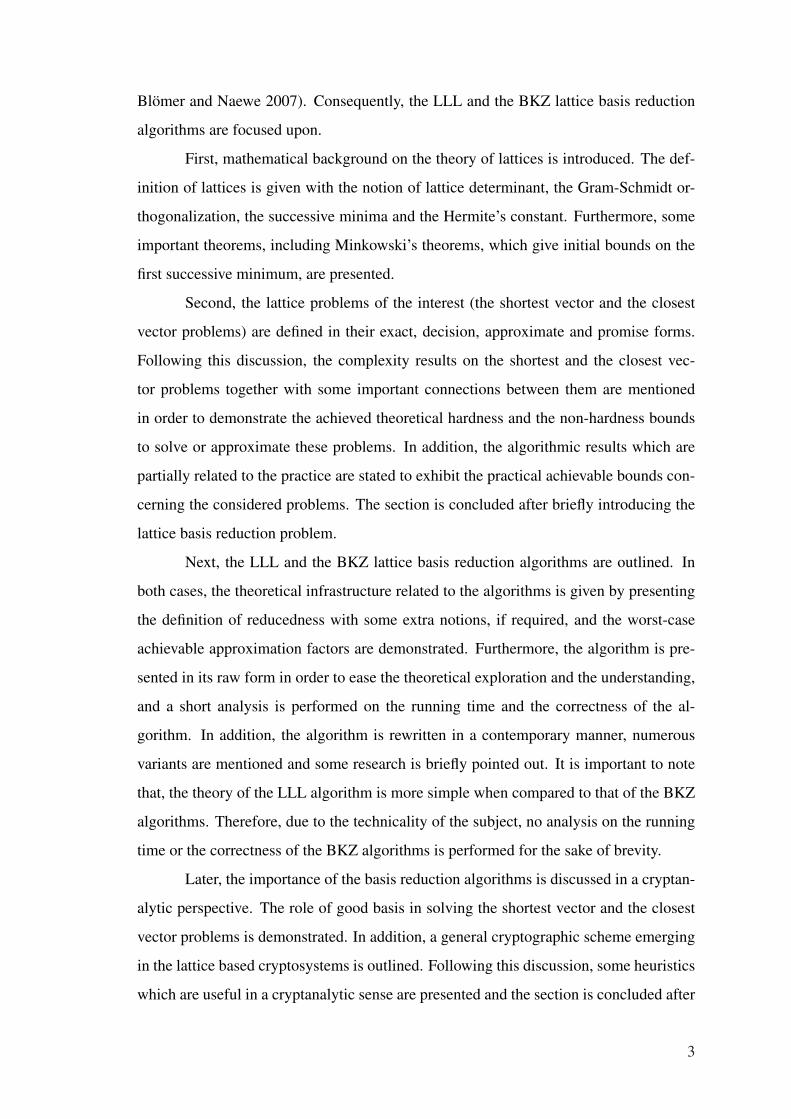
Next, the LLL and the BKZ lattice basis reduction algorithms are outlined. In
both cases, the theoretical infrastructure related to the algorithms is given by presenting
the definition of reducedness with some extra notions, if required, and the worst-case
achievable approximation factors are demonstrated. Furthermore, the algorithm is pre-
sented in its raw form in order to ease the theoretical exploration and the understanding,
and a short analysis is performed on the running time and the correctness of the al-
gorithm. In addition, the algorithm is rewritten in a contemporary manner, numerous
variants are mentioned and some research is briefly pointed out. It is important to note
that, the theory of the LLL algorithm is more simple when compared to that of the BKZ
algorithms. Therefore, due to the technicality of the subject, no analysis on the running
time or the correctness of the BKZ algorithms is performed for the sake of brevity.
Later, the importance of the basis reduction algorithms is discussed in a cryptan-
alytic perspective. The role of good basis in solving the shortest vector and the closest
vector problems is demonstrated. In addition, a general cryptographic scheme emerging
in the lattice based cryptosystems is outlined. Following this discussion, some heuristics
which are useful in a cryptanalytic sense are presented and the section is concluded after
3

discussing the lattice based attacks on relatively more general lattice based cryptographic
schemes.
Next, the most efficient variants of the LLL algorithm and the BKZ algorithm are
considered for a practical assessment regarding a common runtime parameter belonging
to the algorithms. It is important to note that, these variants are based on some certain
heuristics and in general have no theoretical inspections. However, they are also the most
preferred algorithms in practice and by the cryptanalysts due to their efficiency.
Finally, the study is concluded by presenting some remarks concerning this and
possible future research.
4

CHAPTER 2
BACKGROUND
In this chapter, basic information on the lattices is conveyed. The fundamental
definitions and important theorems related to the point lattices are presented keeping the
discussion as simple and concise as possible.
2.1. Lattice and Basis
A lattice is the set of all integral combinations of n linearly independent vectors
b1, ...,bn ∈ Rm denoted by
Λ = L(b1, . . . ,bn) =
{n
∑i=1
xibi : xi ∈ Z,bi ∈ Rm
}(2.1)
or
Λ = L(B) ={
Bx : B ∈ Rm×n,x ∈ Zn} (2.2)
where B = {b1, . . . ,bn} is called the lattice basis and B = [b1 . . .bn]∈Rm×n is the matrix
representation of the basis with columns as the basis vectors. The integers n and m are
called lattice dimension (or rank), dim(Λ), and lattice degree, deg(Λ), respectively, and
when n = m the lattice is called full dimensional. Without any references to a specific
basis, lattice Λ can be defined to be a nonempty discrete subset of Rm which is closed
under subtraction. Consequently, lattices are discrete additive subgroups of Rm.
Linear span of the basis vectors is defined as
span(B) = {Bx : x ∈ Rn} . (2.3)
Since all the bases of the same lattice generate the same span, we can define the span of
the lattice as span(Λ). It is obvious that
dim(Λ) = dim(span(Λ)) (2.4)
and span(Λ) = Rm if and only if the lattice is full dimensional.
5

Half open parallelepiped associated with a lattice basis B is defined as
P(B) ={
Bx : B ∈ Rm×n,xi ∈ [0,1)}
(2.5)
It should be noted that if B′ is another lattice basis then P(B′) does not contain any lattice
vectors other than zero.
Two lattice bases B and B′ generate the same lattice if and only if there exist
an integral matrix U with |det(U)| = 1 such that B′ = BU. U is also called unimodular
matrix, and the bases B and B′ are said to be equivalent. The statement can be proved
using the half open parallelepipeds.
2.2. Determinant
For all x,y∈Rm and a∈R, a norm is a function ‖.‖ :Rm→R, which is generally
used to measure length, such that
• It is positive definite, i.e. ‖x‖> 0 for x 6= 0 and ‖0‖= 0.
• It is homogeneous, i.e. ‖ax‖= |a| · ‖x‖.
• It satisfies the triangle inequality, i.e. ‖x+y‖6 ‖x‖+‖y‖.
Furthermore, for any p > 1, the family of norm functions, lp norms, are defined as
‖x‖p =
(m
∑i=1|xi|p
)1/p
(2.6)
Note that l2 norm is the Euclidean norm whereas l∞ norm is called the maximum norm
since
‖x‖∞ = limp→∞
‖x‖p =m
maxi=1
|xi| . (2.7)
Related to the norm distance between two vectors is
dist(x,y) = ‖x−y‖ . (2.8)
Gram-Schmidt orthogonalization process is almost always referred while study-
ing the lattices. For any sequence of vectors b1, ...,bn, the Gram-Schmidt orthogonalized
vectors are defined as
b∗i = bi−i−1
∑j=1
µi, jb∗j (2.9)
6
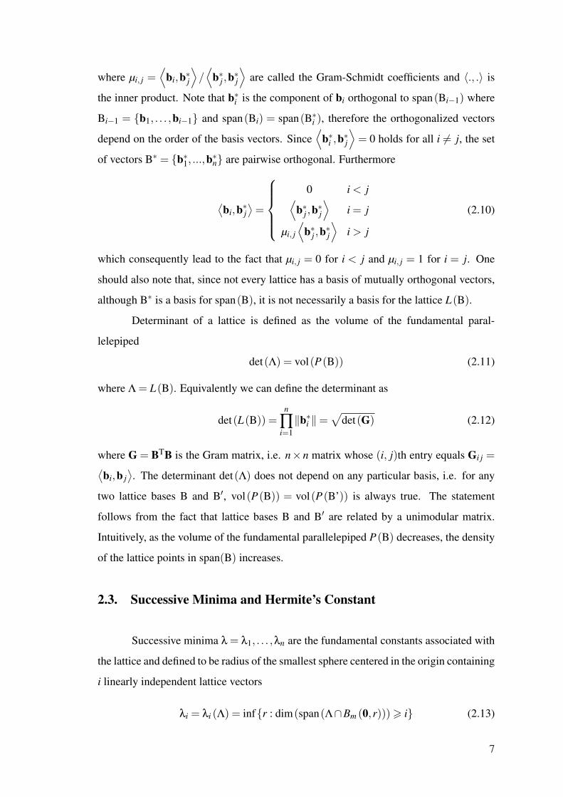
where µi, j =⟨
bi,b∗j⟩
/⟨
b∗j ,b∗j⟩
are called the Gram-Schmidt coefficients and 〈., .〉 is
the inner product. Note that b∗i is the component of bi orthogonal to span(Bi−1) where
Bi−1 = {b1, . . . ,bi−1} and span(Bi) = span(B∗i ), therefore the orthogonalized vectors
depend on the order of the basis vectors. Since⟨
b∗i ,b∗j⟩
= 0 holds for all i 6= j, the set
of vectors B∗ = {b∗1, ...,b∗n} are pairwise orthogonal. Furthermore
⟨bi,b∗j
⟩=
0 i < j⟨b∗j ,b∗j
⟩i = j
µi, j
⟨b∗j ,b∗j
⟩i > j
(2.10)
which consequently lead to the fact that µi, j = 0 for i < j and µi, j = 1 for i = j. One
should also note that, since not every lattice has a basis of mutually orthogonal vectors,
although B∗ is a basis for span(B), it is not necessarily a basis for the lattice L(B).
Determinant of a lattice is defined as the volume of the fundamental paral-
lelepiped
det(Λ) = vol(P(B)) (2.11)
where Λ = L(B). Equivalently we can define the determinant as
det(L(B)) =n
∏i=1‖b∗i ‖=
√det(G) (2.12)
where G = BTB is the Gram matrix, i.e. n×n matrix whose (i, j)th entry equals Gi j =⟨bi,b j
⟩. The determinant det(Λ) does not depend on any particular basis, i.e. for any
two lattice bases B and B′, vol(P(B)) = vol(P(B’)) is always true. The statement
follows from the fact that lattice bases B and B′ are related by a unimodular matrix.
Intuitively, as the volume of the fundamental parallelepiped P(B) decreases, the density
of the lattice points in span(B) increases.
2.3. Successive Minima and Hermite’s Constant
Successive minima λ = λ1, . . . ,λn are the fundamental constants associated with
the lattice and defined to be radius of the smallest sphere centered in the origin containing
i linearly independent lattice vectors
λi = λi (Λ) = inf{r : dim(span(Λ∩Bm (0,r))) > i} (2.13)
7

where Bm (0,r) is the m dimensional open ball of radius r around the origin 0. There
always exist linearly independent lattice vectors achieving the successive minima, i.e.
there exist linearly independent x1, . . . ,xn ∈Λ such that ‖xi‖= λi. Therefore, successive
minima can also be defined as
λi = λi (Λ) = min{
r : dim(span
(Λ∩Bm (0,r)
))> i
}(2.14)
where Bm (0,r) is the m dimensional closed ball of radius r around the origin 0.
Related to the determinant and the first minimum of the lattice, the Hermite’s
constant is defined as follows
γn = maxλ1 (Λ)2
det(Λ)2/n(2.15)
when Λ ranges over all n dimensional lattices. The Hermite’s constant of dimension n
has the following bounds
n2πe
+log(πn)
2πe+o(1) 6 γn 6 1.744n
2πe(1+o(1)) . (2.16)
Furthermore, γ2 = 4/3 and γn 6 (2/3)n for all n > 2.
2.4. Important Theorems
Theorem 2.1. Let B be a lattice basis and B∗ be the corresponding Gram-Schmidt or-
thogonalization. Then
λ1 >n
mini=1
‖b∗i ‖> 0. (2.17)
The theorem proves a lower bound on the first successive minimum. The proof
can be carried out by evaluating the expression 〈Bx,b∗i 〉 where x ∈ Zn by letting i be
the largest index such that xi 6= 0 and showing |〈Bx,b∗i 〉| > ‖b∗i ‖2 by using the fact that
|〈Bx,b∗i 〉|6 ‖Bx‖‖b∗i ‖.
Theorem 2.2. Let Λ be a lattice of rank n. There exist linearly independent lattice
vectors vi for i = 1, . . . ,n such that
‖vi‖= λi. (2.18)
In order to show that there exist a lattice vector achieving the first minimum,
one can use the closed ball Bm (0,2λ1). Since the closed ball is a compact set one can
8

extract a convergent subsequence of lattice vectors with their limit equals to w such that
‖w‖ = λ1 and then one can prove that w is a lattice vector belonging to the sequence.
By generalizing this approach, the theorem can be proved for all successive minima.
Theorem 2.3. (Blichfeldt Theorem) Let Λ be a lattice and S⊆ span(Λ) be a measurable
set. If vol(S) > det(Λ) then there exist distinct z1,z2 ∈ S such that z1− z2 ∈ Λ.
It is possible to prove the theorem by using the translated parallelepipeds
Px (B) = x + P(B) for all x ∈ Λ. If one lets Sx = S∩Px (B) and S′x = Sx − x, using
the assumption that vol(S) > det(Λ), it can be seen S′x are not pairwise disjoint. There-
fore, there exist z ∈ S′x ∩S′y with z1 = z + x ∈ Sx and z2 = z + y ∈ Sy. Consequently,
z1− z2 = x−y ∈ Λ.
Theorem 2.4. (Minkowski’s Convex Body Theorem) Let Λ be a lattice of rank n and
S ⊂ span(Λ) be a convex set symmetric about the origin. If vol(S) > 2n det(Λ) then
there exist a nonzero lattice vector v ∈ S∩Λ−{0}.
This theorem is a corollary to the Blichfeldt theorem. For the set S symmetric
about the origin with vol(S) > 2n det(Λ), one can define another set S′ = {x : 2x ∈ S}with vol(S’) > det(Λ). At this point one can find distinct vectors such that z1,z2 ∈ S’
. Due to symmetricity of S, −2z2 ∈ S . By convexity of S and the Blichfeldt Theorem,
one can state that nonzero (2z1−2z2)/2 = z1− z2 is in both S and Λ.
Theorem 2.5. (Minkowski’s First Theorem) Let Λ be a lattice of rank n. The first mini-
mum satisfies the following inequality
λ1 6√
ndet(Λ)1/n . (2.19)
In order to obtain the inequality, the convex body theorem can be applied on a
n dimensional sphere S of radius√
ndet(Λ)1/n in span(Λ) centered at the origin. It is
obvious that vol(S) > 2n det(Λ) since the sphere contains n dimensional hypercube with
the edges of length 2n det(Λ)1/n (or more accurately, n dimensional sphere of radius
r has the volume πn/2Γ(n/2+1)rn). Therefore, by convex body theorem, the sphere
contains a nonzero lattice vector.
Theorem 2.6. (Minkowski’s Second Theorem) Let Λ be a lattice of rank n. The succes-
sive minima satisfy the following inequality(
n
∏i=1
λi
)1/n
6√
ndet(Λ)1/n . (2.20)
9

To prove the theorem, one can define a transformation using the Gram-Schmidt
orthogonalized vectors T(∑cix∗i ) = ∑λicix∗i where ‖xi‖= λi for all i. Using T, n dimen-
sional unit sphere S in span(Λ) can be transformed to the symmetric convex body T(S).
Assuming that the inequality in the theorem is not correct gives vol(T(S)) > 2n det(Λ).
Hence T(S) contains a nonzero lattice vector y. Letting k be the largest index i such that
ci 6= 0 in y = ∑λicix∗i = T(∑cix∗i ) = T(x) and k′ be the smallest index such that λk′ = λk
, one can see that y is linearly independent from x1, . . . ,xk′−1 and ‖y‖ 6 λk ‖x‖ < λk.
Consequently, x1, . . . ,xk′−1,y form k′ linearly independent vectors of length < λk′ = λk
contradicting the definition of k′th successive minimum. Therefore the assumption is
wrong and the inequality in theorem holds.
Minkowski’s theorems have stronger (or generalized) forms. To mention them
briefly, for any lattice of rank , the following statements hold.
• λ1 6√γn det(Λ)1/n
•(
n∏i=1
λi
)1/n
6√γn det(Λ)1/n
where γn is the Hermite’s constant.
2.5. Referential
For more information on lattices, complete proofs and generalized or stronger
versions of the theorems, reader might refer to the texts on the geometry of numbers,
such as (Gruber and Lekkerkerker 1987, Siegel 1989, Lagarias 1995, Cassels 1997, Sil-
verman 2006, Coppel 2006).
10

CHAPTER 3
LATTICE PROBLEMS
The purpose of this chapter is to give brief information on the lattice related
problems of interest. The problems discussed here are the shortest vector and the closest
vector problem in lattices. In addition, the complexity and the algorithmic results related
to mainly these problems are mentioned.
3.1. SVP and CVP
There are many problems related to the lattices. Finding the shortest lattice vector
and finding the closest lattice vector to a given target point are two such problems which
only have exponential time algorithms to solve them in an exact manner.
Definition 3.1. (Shortest Vector Problem - SVP) Given a lattice Λ, find a nonzero lattice
vector x ∈ Λ−{0} such that ‖x‖6 ‖y‖ for all y ∈ Λ−{0}.
Definition 3.2. (Closest Vector Problem - CVP) Given a lattice Λ and a target vector t,
find a lattice vector x ∈ Λ such that ‖x− t‖6 ‖y− t‖ for all y ∈ Λ .
In order to study the problems in depth, different versions of the problems which
capture different algorithmic tasks are defined. The search problems capture the task
of finding a particular lattice vector which is nonzero and the shortest (in SVP) or the
closest vector to the given point (in CVP). Whereas, the optimization problems consist of
finding the minimum of the norms of all lattice vectors (in SVP) or the minimum value
of the distance between the lattice and the target point (in CVP). Finally, the decision
problems are based on deciding whether there exists a lattice vector with norm smaller
than or equal to a given positive rational value or whether there exists a lattice vector
whose distance to the target point is less than or equal to the given positive rational value.
The search problems are more difficult than the other versions since they include finding
the specific vectors, whereas the decision problems are the easiest. For this reason, all
the hardness results hold for decision problems.
11
Due to the hardness of these problems, approximate versions, which return so-
lutions within some specified factor from the optimal, are defined below (with a little
change in the representation).
Definition 3.3. (Approximate SVP - SVPγ) Given a lattice basis B ∈ Zm×n, find a
nonzero lattice vector Bx where x ∈ Zn − {0} such that ‖Bx‖ 6 γ‖By‖ for all y ∈Zn−{0}.
Definition 3.4. (Approximate CVP - CVPγ) Given a lattice basis B ∈ Zm×n and a target
vector t ∈ Zm, find a lattice vector Bx where x ∈ Zn such that ‖Bx− t‖6 γ‖By− t‖ for
all y ∈ Zn.
Note that the above problems are defined on integer lattices. This mainly stems
from the fact that from a computational perspective the representation of real numbers
are limited to a subset of rational numbers and every rational lattice has an equivalent
integer lattice representation.
The approximation factor γ is generally defined as a function of the lattice di-
mension (or rank) although it can be a function of any parameter related to the lattice.
The best known polynomial time algorithms achieve approximation factors exponential
in the rank of the lattice.
Definition 3.5. (GapSVPγ) Given an instance (B,r) where lattice basis B ∈ Zm×n and
rational number r ∈Q. For γ is a function of the rank,
• (B,r) is a YES instance if ‖Bz‖6 r for some z ∈ Zn−{0}.
• (B,r) is a NO instance if ‖Bz‖> γr for all z ∈ Zn−{0}.
Definition 3.6. (GapCVPγ) Given an instance (B, t,r) where lattice basis B ∈ Zm×n,
target vector t ∈ Zm and rational number r ∈Q. For γ is a function of the rank,
• (B, t,r) is a YES instance if ‖Bz− t‖6 r for some z ∈ Zn.
• (B, t,r) is a NO instance if ‖Bz− t‖> γr for all z ∈ Zn.
It is possible to define r to be a real number because the real r can always be
replaced with a proper rational approximation. For example, in l2 norm a real r can
always be replaced by a rational number in[r,√
r2 +1)
.
12

Note that, when γ = 1, SVPγ and CVPγ are equivalent to SVP and CVP, and
GapSVPγ and GapCVPγ are equivalent to the decision problems associated with SVP
and CVP respectively. Furthermore, if one has an access to an algorithm which solves
SVPγ (CVPγ) then one can easily solve GapSVPγ (GapCVPγ) using this algorithm. On
the other hand, if one has an access to a decision oracle solving GapSVPγ (GapCVPγ),
one can solve SVPγ (CVPγ).
Another important remark is that, even if one manages to find a shortest (or a
closest) lattice vector, there is no known polynomial time proof (certificate) which shows
it is indeed a shortest (or closest) lattice vector.
3.2. Summary of Complexity Results
There have been several researches on the complexity of lattice problems. Here,
the research regarding SVP and CVP is summarized. The topics of interest are the
hardness results, which, in a sense, provide lower bounds in order to efficiently approx-
imate the mentioned problems and the non-hardness results, which presents the factors
in which the related problems do not seem to be hard. The results for l∞ norm are men-
tioned separately due to the similarities between the earlier findings on the problems
with respect to this norm. Furthermore, some studies on the relations between SVP and
CVP are also referred.
For good surveys on the complexity of lattice problems reader may refer to (Cai
1999, 2000, Regev 2007).
3.2.1. SVP Hardness
Ajtai (1996) presents significant worst-case to average-case connection (reduc-
tion) for some special versions of SVP, which states that if there is no algorithm to ap-
proximate (decisional) SVP within some polynomial factor for any lattice, then (search)
SVP is hard to solve exactly when the lattice is chosen randomly according to a certain
distribution. This type of connection currently does not exist in any other problem in NP
and is believed to be outside P. Later, Ajtai (1998) also proves the NP-hardness of SVP
(with respect to the l2 norm) under randomized reductions, being a breakthrough initi-
13

ating several studies on SVP and other lattice problems. In the same paper, Ajtai shows
that approximating SVP to within factors 1 + 2−nε, for some absolute constant ε > 0,
with respect to the l2 norm is NP-hard for randomized reductions and the corresponding
decision problem is NP-complete for randomized reductions.
Cai and Nerurkar (1997, 1999) improve the results of Ajtai by improving the
worst-case to average-case connection and by demonstrating the NP-hardness of ap-
proximating SVP to within a factor 1+n−ε, for ε > 0, under randomized reductions and
with respect to the lp norms where 1 6 p < ∞.
Micciancio (1998, 2001b) further improves the hardness results and shows that
in any lp norm SVP is NP-hard to approximate to within any constant factor less than
21/p (in particular√
2) under randomized reductions. In the same paper, Micciancio
also shows that a proper NP-hardness result (hardness under deterministic many-one
reductions) can be obtained under a certain reasonable number theoretic conjecture.
Kumar and Sivakumar (1999) show that the problem of deciding whether there
exist a lattice vector shorter than a given rational is NP-hard under randomized reduc-
tions. The result holds even the lattice has exactly zero or one such vector.
Khot (2003) presents a new hardness of approximation result for SVP under
the assumption NP 6⊆ ZPP. The result is to within a factor of p1−ε, for ε > 0, with
respect to lp norm for large enough constant p = p(ε). Furthermore, in (Khot 2005),
the author improves the results in (Micciancio 2001b, Khot 2003) by proving that there
is no polynomial time algorithm approximating SVP in lp, norm where 1 < p < ∞ to
within any constant factor under the assumption NP 6⊆RP and that there is no polynomial
time algorithm approximating SVP in lp, 1 < p < ∞, norm with approximation ratio
2log0.5−ε n, ε > 0 is an arbitrarily small constant, under the stronger assumption that NP 6⊆RTIME
(2poly(logn)
). Although, Khot’s proof does not work for l1 norm, Regev and
Rosen (2006) impliy that it also hold for p = 1 .
Haviv and Regev (2007) improve the approximation factor in (Khot 2005) to
an almost-polynomial level, 2log1−ε n for any ε > 0 under lp norm where 1 6 p <
∞. Furthermore, the authors also show that under the (stronger) assumption NP 6⊆RSUBEXP = ∩
δ>0RTIME
(2nδ
)the hardness factor is nc/ log logn for some constant c > 0.
On the other hand, there has been some research on lattice problems addressing
particular quantum-related concepts. Regev (2004c) presents the first explicit connec-
14

tion between quantum computation and lattice problems, particularly on SVP. Later,
Aharonov and Regev (2003) give the first non-trivial upper bound on the quantum com-
plexity of a lattice problem by showing that coGapSVP (a Gap version of SVP which
has been known to be in AM∩ coNP but not known to be in NP or MA) lies in QMA,
the quantum analogue of NP. Also, Regev (2005) gives a quantum reduction from worst
case lattice problems SVP and SIVP (shortest independent vectors problem) to a certain
learning problem and proposes a public key cryptosystem whose security is based on the
hardness of the learning problem and so on the worst-case quantum hardness of SVP and
SIVP.
3.2.2. CVP Hardness
van Emde Boas (1981) is the first one to establish the NP-hardness of CVP, and
Kannan (1987b, 1983) gives a more natural proof of this result.
Arora et al. (1997) prove that approximating CVP within a constant factor in
any lp norm is NP-hard. They also show that approximating CVP to within a fac-
tor of 2log0.5−ε n for ε > 0, is hard, unless NP is in quasi-polynomial deterministic time
DTIME(npoly( logn)).
Dinur et al. (1998) show that CVP in lattice is NP-hard to approximate to
within almost-polynomial factors, more accurately any factor up to 2log1−ε n where
ε = (log logn)−a for any constant a < 1/2, improving (Arora, et al. 1997). Furthermore,
together with Raz, they prove that CVP is NP-hard to approximate to within nc/ log logn
for some constant c > 0 with respect to the lp norms where 1 6 p < ∞ (Dinur, et al.
2003).
Cai (2001) establishes a worst-case to average-case connection for CVP. Thus,
an evidence of average-case hardness of CVP is provided.
3.2.3. SVP and CVP Non-hardness
Lagarias at al. (1990) state that approximating SVP or CVP to within a factor of
cn, for an appropriate constant c, cannot be NP-hard, unless NP = coNP. Furthermore,
combining (Lagarias, et al. 1990, Hastad 1988, Banaszczyk 1993) shows that SVP and
15

CVP within n is in NP∩ coNP. Therefore, a factor n NP-hardness would imply that
NP = coNP.
Goldreich and Goldwasser (2000) prove that approximating SVP or CVP, under
the smart Cook reductions, to within a factor of√
n, more specifically√
n/ logn, is
unlikely to be NP-hard since the problem lies in NP∩ coAM and an NP-hardness with
such factors would imply coNP⊆ AM.
Cai (1998) simplifies the proof of the argument in (Lagarias, et al. 1990), and
states that finding a n1/4-unique shortest vector is not NP-hard under polynomial time
many-one reductions, unless the polynomial time hierarchy collapses. In addition, in
(Cai and Nerurkar 2000), it is shown that the arguments in (Goldreich and Goldwasser
2000) is also valid even under general Cook reductions.
Aharonov and Regev (2005) improve the factor n non-hardness result and show
that approximating SVP or CVP to within a factor of c√
n, for some c > 0, lies in
NP∩ coNP, meaning that achieving a c√
n NP-hardness would imply that NP = coNP.
Furthermore, following the results of Goldreich and Goldwasser (2000), the authors re-
mark that approximating SVP or CVP to within a factor of c√
n/ logn is likely to be
NP∩ coNP.
3.2.4. Results in l∞ Norm
It is notable that SVP and CVP behave similarly with respect to the l∞ norm and
they seem to be more difficult. NP-hardness of SVP and CVP with respect to the l∞
norm is established by van Emde Boas (1981).
Arora et al. (1997) state that approximating SVP in l∞ norm to within a fac-
tor of 2log0.5−ε n for ε > 0, is hard, unless NP is in quasi-polynomial deterministic time,
DTIME(npoly( logn)). In the same paper, the result is proved to hold for CVP in any lp
norm, in particular CVP in l∞ norm. Furthermore, it is shown that improving the factor
to√
n would imply the hardness of SVP in l2 norm.
Dinur (2000) shows that SVP and CVP under norm l∞ is NP-hard to approximate
to within an almost-polynomial factor n1/ log logn, improving the results of Arora et al.
(1997), and, in (Dinur 2002), further generalizes the result by proving that SVP and
CVP with respect to the l∞ norm is NP-hard to approximate to within almost-polynomial
16

factors nc/ log logn for some constant c > 0.
Goldreich and Goldwasser (2000) give non-hardness result on SVP and CVP
with respect to l∞ norm showing that n/ logn factor NP-hardness for SVP or CVP in l∞
norm would imply the collapse of polynomial time hierarchy.
3.2.5. SVP-CVP Reductions
Some of the important results regarding the reductions between SVP and CVP
can be briefly and chronologically listed as follows.
Kannan (1987a) provides a link relating approximating SVP to approximating
CVP. Approximating CVP to a factor of n3/2 f (n)2 is polynomial time Turing reducible
(Cook reducible) to approximating SVP to a factor of f (n) for any nondecreasing func-
tion f (n). Also, the author proves that approximating CVP to within a factor of√
n/2
is polynomial time Cook reducible to the decision version of SVP (Kannan 1987b).
Henk (1997) shows with respect to certain class of norms there exist a polynomial
time Turing, more specifically Cook, reduction from SVP to CVP.
Goldreich et al. (1999) show that approximating SVP is not harder than approxi-
mating CVP by presenting a direct reduction from SVP to CVP which preserves the fac-
tor of approximation and lattice dimension. Specifically, given an oracle which solves
f (n)-approximate CVP, one can solve f (n)-approximate SVP in polynomial time.
Ajtai et al. (2002) present a 2O(n) time Turing reduction from approximate CVP
to SVP.
3.3. Summary of Algorithmic Results
As already mentioned, there is no polynomial time algorithm solving SVP or
CVP. Furthermore, there is no known such algorithm to approximate these problems to
within a polynomial factor. The best polynomial time algorithms achieve slightly sub-
exponential factors. In this section, main algorithmic results for (approximately) solving
SVP and CVP are summarized.
17

3.3.1. Approximating SVP
Lenstra et al. (1982) describe and analyze a lattice basis reduction algorithm
by improving the Lenstra’s algorithm in (Lenstra 1981). The algorithm is came to be
known as LLL (Lenstra Lenstra Lovasz) algorithm and it has several variants such as
(Schonhage 1984, Schnorr 1988, Schnorr and Euchner 1994, Storjohann 1996, Koy and
Schnorr 2001a,b, Akhavi 2002, Koy and Schnorr 2002, Schnorr 2006b, Nguyen and
Stehle 2007). Roughly, LLL algorithm can be used to approximate SVP to within a
factor of 2(n−1)/2 performing O(n4 logB
)number of arithmetic operations on integers of
binary length O(n logB), where B is the squared norm bound of the input basis vectors.
On the other hand, it is also possible to achieve the provable approximation factor up
to α(n−1)/2, where α ≈ 4/3, by choosing the parameters for basis reduction differently,
while preserving the practicality. It is true that α(n−1)/2 6∼ 1.153n for α ≈ 4/3. The
factor of approximation can be decreased to for lattices with high density where λ21 ≈
γn det(Λ)2/n. Furthermore, for random lattices in (Nguyen and Stehle 2006), the value
of α can be decreased to ≈ 1.08 on the average for the LLL in (Lenstra, et al. 1982),
and to ≈ 1.05 on the average for the LLL with deep insertions in (Schnorr and Euchner
1994). See (Nguyen and Stehle 2006, Schnorr 2006a).
Schnorr (1987) defines a family of reduction algorithms from LLL to HKZ
(Hermite Korkine Zolotarev) reduction, named BKZ (Block Korkine Zolotarev), whose
performance depends on , the blocksize, parameter. The author improves and uses
the (HKZ) reduction algorithm proposed by Kannan (1983) in order to obtain poly-
nomial time algorithms to approximate SVP. Schnorr’s blockwise lattice basis reduc-
tion algorithm runs in O(
n2(
kk/2+o(k) +n2)
logB)
arithmetic operations performed on
O(n logB) bit integers. The algorithm approximates SVP to within a factor of(6k2)n/(2k)
where assuming the unproven bound γk 6 k/6 for k > 24 , one obtains a factor of
(k/3)n/k. Gama et al. (2006) show the factor to be (βk/δ)(n−1)/(2k) where βk is a con-
stant related to BKZ reduced bases and δ≈ 1. As stated by Schnorr (2006a), for k = 24,
this factor is < 1.165(n−1)/2 which, under the heuristic in (Schnorr 2003), improves
to 6 α(n−1)/2 where α ≈ 1.034. Furthermore, for the proper choice of the blocksize,
k = O(logn/ log logn), one can achieve a 2O(n(log logn)2/ logn) approximation factor.
18
Kumar and Sivakumar (2001) show a 2O(n/ε) time algorithm which approximates
SVP to within a factor n3+ε for arbitrary ε > 0.
Ajtai et al. (2001), based on (Kumar and Sivakumar 2001), present a probabilis-
tic sieve algorithm which finds the shortest vectors. Using this algorithm in Schnorr’s
BKZ basis reduction algorithm, it is possible to achieve 2O(n log logn/ logn) approximation
to SVP in randomized polynomial time for k = O(logn). Furthermore, as stated by
Schnorr (2001), assuming the unproven bound γk 6 k/6 for k > 24 and combining the
sieve algorithm with the reduction algorithm in (Koy 2004) yields a factor of (k/6)n/k in
O(
n22O(k) +n4)
time storing 2O(k) lattice vectors.
Schnorr (2003) describes an algorithm which approximates SVP to within
(k/6)n/2k in O(
n3 (k/6)k/4 +n4)
time by iterating random sampling of short lattice
vectors. In addition, it is stated that the algorithm can be improved using some par-
ticular additional heuristics at the expense of increased space complexity. Inspired by
Ajtai et al. (2001), the author also presents a sieve algorithm to approximate SVP to
within a factor of k(3n)/(4k) in O(n320.835k +n4) time storing 20.835k +O(n) lattice vec-
tors. Furthermore, comparisons with the other approximation algorithms are performed,
and some refinements are proposed on the results in (Schnorr 2001).
Koy (2004) introduces a blockwise lattice basis reduction for approximating
SVP. The algorithm achieves a proven factor of(αγ2
k
)n/k−1 where γk is the Hermite’s
constant and α≈ 4/3 (for k = 48 approximation factor is proven to be ≈ 1.075(n−1)/2).
The algorithm runs in O(
n3m log1/δ 2)
+ n3kO(k) arithmetic steps where δ ≈ 1 and the
runtime is also expressed as O(
n3kk/2+o(k) +n4)
time. Assuming the unproven bound
γk 6 k/6 for k > 24, the factor becomes (k/6)n/k. In addition, under the heuristic of
Schnorr (2003), the factor can be improved to ≈ (1.034)(n−1)/2. Moreover, it is possible
to further decrease the approximation factor to ≈ (1.025)(n−1)/2 for k = 80 by replacing
the HKZ reduction by the random sampling reduction in (Schnorr 2003) under the same
heuristic. The details of the Koy’s algorithm can also be found in (Schnorr 2006a).
Blomer and Naewe (2007) obtain single-exponential time 1 + ε approximation
algorithm for SVP requiring ((2+1/ε)n b)O(1) arithmetic operations where ε > 0 is ar-
bitrary.
Gama and Nguyen (2008a) present a deterministic and a probabilistic algorithm
which perform γ(n−k)/(k−1)k approximation to SVP. The deterministic algorithm is an im-
19

provement of the algorithms in (Schnorr 1987, Gama, et al. 2006) and achieves a factor
of 2O(n(log logn)2/ logn) for k = O(logn/ log logn) in polynomial time. Whereas the prob-
abilistic algorithm, using the randomized algorithm of Ajtai et al. (2001) within blocks
of size k, solves SVP to within a factor of 2O(n(log logn)/ logn) for k = O(logn/ log logn)
in polynomial time.
As a last remark on the approximation algorithms, Gama and Nguyen (2008b)
notes that it seems reasonable to assume that current algorithms, namely LLL, BKZ and
their particular variants, should achieve in a reasonable time an approximation factor 61.01n on the average, and 6 1.02n in the worst case based on the extensive experiments.
This is an important assessment of the optimistic behaviour of the lattice basis reduction
algorithms, i.e. the lattice basis reduction algorithms generally behave much better than
their proven worst case theoretical bounds in practice.
3.3.2. Solving SVP
Kannan (1983, 1987b) uses LLL in order to solve SVP. The super-exponential
algorithm of Kannan performs nn+o(n)sO(1) arithmetic operations, where s is the length
of the input. The numbers produced in the execution of the algorithm are of binary
length O(n2 (logB+ logn)
). Helfrich (1985) improves the running time of the Kan-
nan’s algorithm for SVP to nn/2+o(n)sO(1) arithmetic operations. In addition, Hanrot and
Stehle (2007, 2008) further analyze the Kannan’s algorithm and show its running time
complexity to be nn/2e+o(n)sO(1) arithmetic operations.
Ajtai et al. (2001) present a sieve algorithm for solving SVP. The algorithm,
which has 2O(n) space bound, can be used to solve SVP (with high probability) in a
randomized 2O(n) time improving 2O(n logn) time bound of Kannan’s algorithm for the
problem. In fact, in 2O(n) time the algorithm finds all approximate vectors with approx-
imation factor greater than or equal to 1. The practicality of the algorithm is shown by
Nguyen and Vidick (2008).
3.3.3. Approximating CVP
Babai (1986) uses LLL to obtain a reduced lattice basis in order to approximate
20

CVP. The author presents two polynomial time algorithms based on two different heuris-
tics. The first algorithm, rounding off algorithm, approximates CVP to within a factor
of 1 + 2n(9/2)n/2 whereas the second algorithm, namely the nearest plane algorithm,
achieves a 2n/2 approximation factor, which can be improved to 2(4/3)n/2.
Schnorr (1996) presents a BKZ version of the nearest plane algorithm. The al-
gorithm can be used to approximate CVP to within a factor of√
nγn/(k−1)k in kO(k) time.
Therefore, for the properly chosen blocksize parameter, the approximation factor be-
comes 2O(n(log logn)2/ logn) in polynomial time. This factor can also be achieved using the
algorithms in (Gama, et al. 2006, Gama and Nguyen 2008a).
Ajtai et al. (2001) obtain an algorithm to solve approximate CVP to within a
factor of√
n/2 in randomized 2O(n) time (combining a 2O(n) time algorithm for SVP
and the polynomial time Turing reduction from approximate CVP to SVP given in
(Kannan 1987a)). In addition, it is possible to approximate CVP to within a factor of
2O(n log logn/ logn) using their randomized polynomial time SVP algorithm and the Kan-
nan’s link presented in (Kannan 1987a). Moreover, in (Ajtai, et al. 2002), they present
a randomized 2O(1+ε−1)n, for arbitrary ε > 0, algorithm which performs (1+ ε) approx-
imation to CVP, using the SVP algorithm from (Ajtai, et al. 2001) as the subroutine.
Hence, they improve the existing time bound of O(n!) for CVP achieved by the deter-
ministic algorithm in (Blomer 2000).
Blomer and Naewe (2007) approximates CVP, in addition to SVP, to within a
factor 1 + ε in probabilistic single-exponential time. The algorithm has the complexity
bound ((2+1/ε)n s)O(1) for arbitrary ε > 0.
3.3.4. Solving CVP
Kannan (1983, 1987b) also presents an algorithm to solve CVP which uses his
algorithm to solve SVP introduced in the same paper. As in the case of SVP, the al-
gorithm performs nn+o(n)sO(1) number of arithmetic operations which is decreased to
nn/2+o(n)sO(1) by Hanrot and Stehle (2007). The numbers produced during the exe-
cution are rational numbers with numerators and denominators having binary length
O(n2 (s+ logn)
).
Blomer (2000) introduces a new technique based on dual HKZ bases. Using
21

this technique, CVP is solved in n!sO(1) time achieving an exponential improvement
(nn/n! ≈ en) over Helfrich’s improvement over Kannan’s algorithm, (Helfrich 1985,
Kannan 1987b).
Klein (2000) proposes an algorithm which runs in nk2+O(1) time and finds the
closest vector to a given target vector under the condition that the distance of the target
vector from the lattice is at most k times the length of the shortest Gram-Schmidt vector.
The result is a generalization of the argument in (Furst and Kannan 1989) where k is
taken to be 1/2.
Agrell et al. (2002) propose an algorithm to solve CVP. They state that the
algorithm is faster than Kannan’s algorithm (Kannan 1987b) by at least a factor of
(2n/πe)n/2.
3.4. Basis Reduction and Other Lattice Problems
It is important to note the algorithms for solving (approximate) SVP / CVP, do
more that just solving them. These algorithms also produce a reduced basis. Aside from
SVP and CVP, finding a ”good” lattice basis is one of other important problem related
to the lattices. This problem is generally referred to as basis reduction problem. There
is no unique definition of good basis. One could search for a basis where the maximum
of the lengths of its vectors is minimized or one could look for a basis where the product
of the vector lengths is minimized. Many important problems related to the lattice basis
reduction are discussed in (Micciancio and Goldwasser 2002).
For more information on (other) lattice-related problems, such as unique SVP (a
special version of SVP), Hermite-SVP (another variation of SVP), closest vector prob-
lem with preprocessing (CVPP), shortest independent vectors problem (SIVP), shortest
basis problem (SBP) and covering radius problem (CRP) etc, reader may refer to the
resources, including but not limited to, (Ajtai 1996, Blomer and Seifert 1999, Cai 1999,
2000, Micciancio and Goldwasser 2002, Guruswami, et al. 2005, Regev 2005, Haviv
and Regev 2006, Chen and Meng 2006, Blomer and Naewe 2007, Micciancio 2008). In
addition, Regev and Rosen (2006), Peikert (2007) present interesting relations between
lattice problems in l2 norm and the corresponding problems in other lp norms.
22

3.5. Referential
For more information on the complexity, or cryptocomplexity, related issues, one
may refer to textbooks such as (Garey and Johnson 1990, Micciancio and Goldwasser
2002, Rothe 2005).
23

CHAPTER 4
LENSTRA LENSTRA LOVASZ REDUCTION
LLL algorithm which is first proposed by Lenstra et al. (1982) is the first al-
gorithm to approximately solve SVP. The algorithm’s runtime is polynomial and the
achieved SVP approximation factor is exponential in the lattice dimension, more accu-
rately αn/2 where α≈ 4/3. In this chapter, we shall discuss the main aspects of the LLL
algorithm and try to emphasize its importance.
4.1. LLL Reduced Basis
The projection operation is defined as, given x ∈ Rm,
πi (x) =n
∑j=i
⟨x,b j
⟩⟨b j,b j
⟩b∗j (4.1)
where b∗1, . . . ,b∗n are the Gram-Schmidt ortogonalized vectors. The resulting vector πi (x)
is the component of the vector x orthogonal to span(b1, ...,bi−1).
Definition 4.1. (δLLL Reduced Basis) A basis B = [b1 . . .bn] ∈ Rm×n is δLLL reduced
if
•∣∣µi, j
∣∣ 6 12 for all i > j where µi, j = 〈bi,b∗j〉
〈b∗j ,b∗j〉 are the Gram-Schmidt coefficients,
• δ‖πi (bi)‖2 6 ‖πi (bi+1)‖2 where πi (x) is the component of the vector x orthogo-
nal to span(b1, ...,bi−1) and 1/4 < δ < 1 is a real number.
Note that πi (bi) = b∗i and πi (bi+1) = b∗i+1 + µi+1,ib∗i . Furthermore,
since the vectors b1, . . . ,bn are orthogonal we have∥∥b∗i+1 +µi+1,ib∗i
∥∥2 =∥∥b∗i+1
∥∥2 +
|µi+1,i|2 ‖b∗i ‖2. Therefore, if a basis is δLLL reduced then one can write that
δ‖b∗i ‖2 6∥∥b∗i+1
∥∥2 + |µi+1,i|2 ‖b∗i ‖2 . (4.2)
Arranging the inequality one obtains(
δ− 14
)‖b∗i ‖2 6
∥∥b∗i+1∥∥2
. (4.3)
24

By induction on the orthogonalized vectors it is obvious that(
δ− 14
)i−1
‖b∗1‖2 6 ‖b∗i ‖2 . (4.4)
For 1/4 < δ < 1, one can write (δ−1/4)i−1 > (δ−1/4)n−1, and since ‖b∗1‖= ‖b1‖, it
follows that (δ− 1
4
)n−1
‖b1‖2 6 ‖b∗i ‖2 . (4.5)
Combining this with the fact that 0 <n
mini=1
‖b∗i ‖6 λ1, one gets
(δ− 1
4
)(n−1)/2
‖b1‖6 λ1. (4.6)
Consequently,
‖b1‖6(
44δ−1
)(n−1)/2
λ1. (4.7)
Thus, one approximates SVP to within a factor of (4/(4δ−1))(n−1)/2 by δLLL reducing
the basis where 1/4 < δ < 1. Note that for δ = 3/4 the approximation factor becomes
2(n−1)/2 as in (Lenstra, et al. 1982).
In the light of the above discussion, let α = (δ−1/4)−1 then for all LLL reduced
bases one can write
• ‖b1‖2 6 αn−1λ21 and ‖b1‖2 6 αi−1 ‖b∗i ‖2 for all i = 1, . . . ,n,
• ‖b1‖2 6 α(n−1)/2 det(L(B))2/n and ‖b∗n‖2 > α−(n−1)/2 det(L(B))2/n,
using the fact that ‖b∗i ‖2 6 α∥∥b∗i+1
∥∥2. Furthermore, generalizing the discussion in
(Lenstra, et al. 1982), it is possible to obtain
α1−i 6 ‖bi‖2 /λ2i 6 αn−1 (4.8)
for all LLL reduced bases, where i = 1, . . . ,n.
4.2. LLL Basis Reduction Algorithm
The LLL lattice basis reduction algorithm can be seen in Figure 4.1. It is im-
portant to make some remarks on the main points of the algorithm which are crucial in
order to grasp the underlying idea.
Remarks on the reduction step (or the size reduction) of the LLL algorithm shown
in Figure 4.1 can be given as follows:
25

• The reduction is also called the size reduction step and transforms the basis into
an equivalent basis because only elementary (column) operations are performed.
• The Gram-Schmidt orthogonalized vectors associated to the basis before and after
the reduction step remains the same, because if i > j the operation bi ← bi−ab j
does not change the Gram-Schmidt orthogonalization.
• The ith iteration of the outer loop guarantees that∣∣µi, j
∣∣ 6 1/2 for i > j, because
∣∣µi, j∣∣ =
∣∣∣∣∣∣
⟨bi− ci, jb j,b∗j
⟩⟨
b∗j ,b∗j⟩
∣∣∣∣∣∣=
∣∣∣∣∣∣
⟨bi,b∗j
⟩⟨
b∗j ,b∗j⟩ −
⟨bi,b∗j
⟩⟨
b∗j ,b∗j⟩
⟨b j,b∗j
⟩⟨
b∗j ,b∗j⟩
∣∣∣∣∣∣6 1
2(4.9)
which follows from the fact that⟨
b j,b∗j⟩
=⟨
b∗j ,b∗j⟩
.
• It is crucial that the inner loop goes from i−1 down to 1.
Furthermore, there are some points to be made on the swap step of the LLL
algorithm:
• The swap step is performed to satisfy the condition δ‖πi (bi)‖2 6 ‖πi (bi+1)‖2 for
all i.
• There might be several pairs violating this condition and which pair is swapped
does not matter in terms of correctness of the algorithm. In fact, it is possible to
swap several disjoint pairs at the same time.
• After the swap the previous steps of the algorithm need to be redone because the
basis might not satisfy the condition∣∣µi, j
∣∣ 6 1/2 anymore.
Let B > ‖bi‖2 ∈ R for 1 6 i 6 n, then the LLL algorithm has the following
properties.
• SVP approximation factor is α(n−1)/2 where α = (δ−1/4)−1 and 1/4 < δ < 1
(α = 2 for δ = 3/4 and α≈ 4/3 for δ≈ 1).
• Algorithm performs O(n3m logB
)number of arithmetic and O
(n5m log3 B
)bit
operations.
• Integers on which the arithmetic operations are performed have binary length
O(n logB).
26

input : Lattice Basis b1, . . . ,bn ∈ Zm and δ
output: A δLLL reduced basis for the lattice L(B)
(start):
compute b∗1, . . . ,b∗n
(reduction):
for i = 2 to n do
for j = i−1 to 1 do
bi ← bi−[ci, j
]b j where ci, j =
[⟨bi,b∗j
⟩/⟨
b∗j ,b∗j⟩]
end
end
(swap):
if δ‖πi (bi)‖2 > ‖πi (bi+1)‖2 is true for some i then
bi ↔ bi+1
goto (start)
end
output b1, . . . ,bn
Figure 4.1. LLL Lattice Basis Reduction Algorithm.
27

4.3. The Overview of Analysis
This section provides outline on the proof of correctness and the running time
analysis of the LLL algorithm. For the complete proof and analysis, one might refer to
(Lenstra, et al. 1982, Micciancio and Goldwasser 2002, Regev 2004a).
4.3.1. Note on the Correctness
One can easily show that if the algorithm terminates it satisfies the conditions
•∣∣µi, j
∣∣ 6 12 for all i > j
• δ‖πi (bi)‖2 6 ‖πi (bi+1)‖2
using the remarks given in the previous section which hint on the correctness of the
algorithm.
4.3.2. Note on the Running Time
The running time analysis of the algorithm consists of two steps. The first step is
bounding the number of iterations performed by the algorithm, which is exactly the num-
ber of swap operations performed by the algorithm. The second step contains bounding
the running time of each iteration and showing that the size of numbers produced in the
execution of algorithm is also bounded.
In order to bound the number of iterations, one can associate a positive integer
to the lattice basis, let D = ∏ni=1 det(Λi)
2 where Λi = L(b1, . . . ,bi) is the sublattice
generated by the first i basis vectors. It can be shown that the value of D changes only
when the swap occurs. Let Dk+1 be the new value, assuming the vectors bi and bi+1 are
swapped at the kth iteration, it is straightforward to note that Dk decreases by at least by
a factor of δ,Dk+1
Dk=
det(Λ′i)2
det(Λi)2 =
‖πi (bi+1)‖2
‖πi (bi)‖2 < δ. (4.10)
It follows that 1 6 Dk < δkD0 and the number of iterations can be bounded by
k < log1/δ D0 6 1log(1/δ)
n(n−1) log(
nmaxi=1
‖bi‖)
(4.11)
28

which follows from the fact that ‖b∗i ‖6 ‖bi‖ and that D0 6(maxn
i=1 ‖bi‖)n(n−1). Since
log(maxn
i=1 ‖bi‖)
is polynomial in the input size, it can be seen that the number of
iterations is polynomial in the input size for constant δ < 1.
In order to bound the running time of each iteration, one should note that the
number of arithmetic operations performed at each iteration is polynomial. Therefore,
to show a polynomial bound on the running time it is enough to show that the numbers
arising in each iteration can be represented using polynomial number of bits (leading to
the fact that the actual running time which is the number of the bit operations performed
is also polynomial). Since the numbers are rational, one should bound both the precision
and the magnitude.
To bound the precisions of numbers, one can write
〈bi−b∗i ,bk〉=
⟨i−1
∑j=1
vi, jb j,bk
⟩= 〈bi,bk〉=
i−1
∑j=1
vi, j⟨b j,bk
⟩(4.12)
for k < i and vi, j ∈ R. For k = 1, . . . i− 1, there is a system of i− 1 linear equations in
i−1 variables
bTi Bi−1 = vT
i BTi−1Bi−1 (4.13)
where Bk = [b1 . . .bk] and vi = [vi,1 . . .vi,i−1]T. It is possible to interpret vi as the so-
lution vector and BTi−1Bi−1 as the coefficient matrix. Letting di−1 = det(Λi−1)
2 =
detBTi−1Bi−1 ∈ Z when the Cramer’s rule is applied, it can be seen that di−1vi is an
integer vector and therefore di−1b∗i = di−1bi +n∑j=1
di−1vi, jb j is also an integer vector.
This shows that all denominators occurring in b∗i are factors of di−1. In addition,
µi, j =
⟨bi,b∗j
⟩⟨
b∗j ,b∗j⟩ =
d j−1
⟨bi,b∗j
⟩
d j−1
∥∥∥b∗j∥∥∥
2 =
⟨bi,d j−1b∗j
⟩
d j(4.14)
so denominators of µi, j divide d j. Thus, denominators of all rationals divide D = ∏ni=1 di
. Since logD is polynomial in the input size, all denominators occurring in the computa-
tion can be represented using polynomially many bits.
To bound the magnitude of the numbers it is sufficient to show that
‖b∗i ‖2 = di
i−1
∏j=1
(∥∥b∗j∥∥2
)−16 di
i−2
∏j=1
d2j 6 D2 (4.15)
since∥∥∥b∗j
∥∥∥−1
6 d j−1 where d0 = 1, and that
‖bi‖2 = ‖b∗i ‖2 +i−1
∑j=1
µ2i, j
∥∥b∗j∥∥2 6 D2 +(n/4)D2 6 nD2 (4.16)
29
where∣∣µi, j
∣∣ 6 1/2. Concluding that all the quantities occurring in the computation can
be represented with polynomially many bits.
4.3.3. Note on the Approximation Factor
The best approximation factor the algorithm achieves in polynomial time can
be obtained by setting δ = (1/4)+ (3/4)n/(n−1). For such value, δ is closer to 1 than
any constant and the approximation factor is (4/3)n/2. In addition, for sufficiently large
n, the algorithm still has a polynomial running time. See (Micciancio and Goldwasser
2002) for further details.
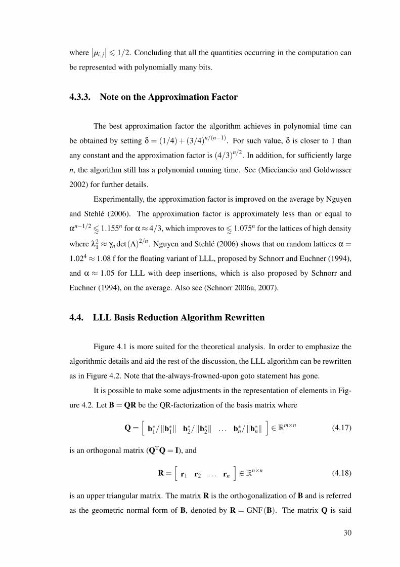
Experimentally, the approximation factor is improved on the average by Nguyen
and Stehle (2006). The approximation factor is approximately less than or equal to
αn−1/2 6∼ 1.155n for α≈ 4/3, which improves to 6∼ 1.075n for the lattices of high density
where λ21 ≈ γn det(Λ)2/n. Nguyen and Stehle (2006) shows that on random lattices α =
1.024 ≈ 1.08 f for the floating variant of LLL, proposed by Schnorr and Euchner (1994),
and α ≈ 1.05 for LLL with deep insertions, which is also proposed by Schnorr and
Euchner (1994), on the average. Also see (Schnorr 2006a, 2007).
4.4. LLL Basis Reduction Algorithm Rewritten
Figure 4.1 is more suited for the theoretical analysis. In order to emphasize the
algorithmic details and aid the rest of the discussion, the LLL algorithm can be rewritten
as in Figure 4.2. Note that the-always-frowned-upon goto statement has gone.
It is possible to make some adjustments in the representation of elements in Fig-
ure 4.2. Let B = QR be the QR-factorization of the basis matrix where
Q =[
b∗1/‖b∗1‖ b∗2/‖b∗2‖ . . . b∗n/‖b∗n‖]∈ Rm×n (4.17)
is an orthogonal matrix (QTQ = I), and
R =[
r1 r2 . . . rn
]∈ Rn×n (4.18)
is an upper triangular matrix. The matrix R is the orthogonalization of B and is referred
as the geometric normal form of B, denoted by R = GNF(B). The matrix Q is said
30

input : Lattice Basis b1, . . . ,bn ∈ Zm and δ
output: A δLLL reduced basis for the lattice L(B)
(initialization):
l ← 1 (l is generally referred as stage)
while l 6 n do
compute the Gram-Schmidt coefficients µl,1, . . . ,µl,l−1 and∥∥b∗l
∥∥2
(size reduce bl against bl−1, . . . ,b1):
for i = l−1 to 1 do
bl ← bl−[µl,i
]bi
(update the Gram-Schmidt coefficients µl,i, . . . ,µl,1):
for j = 1 to i do
µl, j = µl, j−[µl,i
]µi, j
end
end
(swap):
if l 6= 1 and δ∥∥b∗l−1
∥∥2> µ2
l,l−1
∥∥b∗l−1
∥∥2 +∥∥b∗l
∥∥2 then
bl−1 ↔ bl
l ← l−1
else
l ← l +1
end
end
output b1, . . . ,bn
Figure 4.2. LLL Lattice Basis Reduction Algorithm (2).
31

to be isometric, since 〈Qx,Qy〉 = 〈x,y〉 and can be extended to an orthogonal matrix
Q′ ∈ Rm×m. Two bases B and B′ are isometric if and only if GNF(B) = GNF(B′). The
geometric normal form and the LLL reduction are preserved under isometric transforms
Q, i.e. GNF(B) = GNF(QB). Furthermore, due to the fact that⟨bi,b j
⟩=
⟨ri,r j
⟩, µ j,i =
ri, j/ri,i and ‖b∗i ‖ = ri,i, the LLL algorithm can be equivalently written as the algorithm
in Figure 4.3.
Algorithm in Figure 4.3 is notable because it works with the QR-factorization.
This gives the implication that the Gram-Schmidt orthogonalization can be replaced due
to the fact that there are other methods, such as Householder reflections and Givens rota-
tions to compute the QR-factorization, to find the orthogonalized vectors of a given basis.
Therefore, one can substitute the Gram-Schmidt orthogonalization if it is beneficial.
Another important point is that, at the lth stage, LLL performs local LLL reduc-
tions in the swap step on the submatrices rl−1,l−1 rl−1,l
0 rl,l
, (4.19)
and so computes the shortest vector in the 2 dimensional sublattices.
4.5. LLL Variants
The LLL algorithm has many variants. Most remarkable modifications are the
usage of floating point arithmetic numbers, the deep insertions and carrying out the local
reductions on (sub)segments. However, many of such variants have improvable results.
In general, they depend on heuristics for practicality. On the other hand, there also
other variants which are obtained by relaxing or tightening the conditions posed by the
classical LLL algorithm in order to produce at least equivalently good reduced bases.
4.5.1. LLL with Floating Point Arithmetic
A problem with the LLL algorithm is that it uses arithmetic operations on large
integers with O(n logB) bits. In fact, it is somewhat possible to avoid the overhead of
the large integer arithmetic by performing computation using approximate real numbers
and floating point arithmetic. However, this approach comes with stability problems and
32
input : Lattice Basis b1, . . . ,bn ∈ Zm and δ
output: A δLLL reduced basis for the lattice L(B)
(initialization):
l ← 1 (l is the stage)
while l 6 n do
(compute rl =[r1,l, . . . ,rl,l,0, . . . ,0
]T =∥∥b∗l
∥∥[µl,1, . . . ,µl,l,0, . . . ,0
]T ):
for i = 1 to l−1 do
ri,l ←(〈bi,bl〉−∑i−1
k=1 rk,irk,l
)/ri,i
end
rl,l ←∣∣∣‖bl‖2−∑l−1
k=1 r2k,l
∣∣∣1/2
(size reduce bl and rl):
for i = l−1 to 1 do
bl ← bl−[µl,i
]bi
rl ← rl−[ri,l/ri,i
]ri
end
(swap):
if l 6= 1 and δr2l−1,l−1 > r2
l−1,l + r2l,l then
bl−1 ↔ bl
l ← l−1
else
l ← l +1
end
end
output b1, . . . ,bn
Figure 4.3. LLL Lattice Basis Reduction Algorithm (3).
33
in order to preserve sufficient level of accuracy additional measures should be taken.
One such measure is the generalization of the size reduction condition∣∣µi, j
∣∣ 6 η where,
in general, η ∈[1/2,
√δ)
. This stems from the fact that the original size reduction
condition (η = 1/2) can not be achieved when floating point arithmetic numbers are
used. Furthermore, one should also note that the basis should be kept in exact repre-
sentation since the errors occurring in the computation of the basis changes the whole
lattice, therefore cannot be corrected. However, it is possible to recover the other errors
by using a correct basis.
Schnorr (1988) proposes a modification to LLL applying the method of self-
correction to approximate the inverse of a given matrix. The algorithm has provably neg-
ligible floating point errors. The proposed reduction algorithms works on O(n+ logB)
bit integers requiring O(n3m logB
)number of arithmetic steps. Furthermore, when com-
bined with the semi-reduction of Schonhage (1984), the required number of arithmetic
steps decreases to O(n2.5m logB
). On the other hand, Nguyen and Stehle (2007) re-
marks that this algorithm is mostly of theoretical interest and is not implemented widely,
which might possibly be explained by the following reasons: it is not clear which float-
ing point arithmetic model is used, the algorithm is not easy to describe, and the hidden
complexity constants are rather large. More precisely, the required precision of floating
point numbers seems to be higher than 12n+7log2 B.
Schnorr and Euchner (1994) introduce a practical floating point variant of LLL,
named LLLFP, which makes use of floating point arithmetic. The floating point arith-
metic is used to calculate only the Gram-Schmidt coefficients because otherwise the
algorithm would be unstable due to occurring floating point errors and error propaga-
tion. Furthermore, LLLFP introduces different means to correct the errors occurring in
the computation due to the floating point approximations. The produced lattice vectors
are considerably shorter than those of LLL and the algorithm is 10% faster than the prac-
tical versions of the algorithm in (Schnorr 1988). The authors state that LLLFP has a
good stability since it is empirically tested up to dimension 150 using 300 bit integers.
They remark that the algorithm’s stability is good even for single precision floating point
arithmetic for very large numbers and the use of double precision numbers decreases the
number of swaps significantly, and to offset small floating point errors one has to use δ
values greater than 1/4, i.e. δ > 1/2. In addition, as noted by Backes and Wetzel (2001),
34

both the run time and the stability of the algorithm strongly depend on the precision of
the approximations used. High precision approximations cause major loss in efficiency
whereas the small precision causes the algorithm not to terminate due to (accumulated)
floating point errors. Therefore, the algorithm still lacks of efficiency in particular for
large lattice bases or bases with large entries.
Backes and Wetzel (2001) present a heuristic for the LLLFP algorithm proposed
in (Schnorr and Euchner 1994). The key idea is to work with the original lattice basis for
the exact representation so that the problems caused by high precision approximations
can be prevented. The new heuristic allows dynamic adaptation of the floating point
precision thus decreases the run time of the reduction process considerably. The authors
state that the new heuristic is more efficient in reducing large problem instances, allows
a major decrease of the run time and extends the applicability of the Schnorr-Euchner
algorithm such that problem instances that the state-of-the-art method fails to reduce
can be solved. Furthermore, the same authors, in (Backes and Wetzel 2002), present
empirical results on the practical performance of the LLL algorithms, and introduces new
heuristics to improve the LLL variant proposed in (Schnorr and Euchner 1994) together
with test data on these methods. The heuristics developed for the Schnorr-Euchner LLL
strive to speed up the computation, by eliminating the unnecessary operations or doing
operations on shorter operands, and to achieve better reduction results, possibly causing
a decrease in the running time. After performing several tests using the new heuristics,
Backes and Wetzel propose general heuristics for different classes of lattices in order to
determine which variant of the reduction algorithm, for varied parameter choices, yields
the most efficient reduction strategy for reducing a particular problem instance.
Nguyen and Stehle (2007) present a new and natural floating point variant of the
LLL algorithm, namely LL algorithm, which provably outputs an LLL reduced basis
in polynomial time, O(n4m(n+ logB) logB
), using only n log2 3 bit precision which is
independent of logB. The algorithm is called LL because it is is the first LLL algorithm
whose (actual) running time grows only quadratically with respect to n log2 3. The LL
algorithm keep a sufficiently good floating point approximation to the Gram-Schmidt
orthogonalization instead of keeping exact integers and the rational LLL is simulated
by the chosen floating point precision linear in dimension while improving the accuracy
of the usual Gram-Schmidt computations by a systematic use of the Gram matrix. Fur-
35

thermore, size reduction is replaced with a more stable version adapted from Babai’s
nearest plane algorithm. It performs more operations but better suited for floating point
arithmetic.
4.5.2. Deep Insertions
Schnorr and Euchner (1994) also introduce another LLL variant called LLL with
deep insertions or shortly LLLDEEP besides the floating point variant of the LLL algo-
rithm. LLLDEEP replaces and extends the swap step of the classical LLL algorithm by
the deep insertion step to possibly insert the vector bl , called the vector at the lth stage,
to some minimally chosen position i < l. This decreases the norm of the ith vector bi
by at least a factor of√
δ. It is implemented using the floating point arithmetic model
in LLLFP, however exact artihmetic model can also be used. The floating point imple-
mentation of LLLDEEP yields equivalently good results but it is possible that, in the
worst case, it runs in super-polynomial time. Fortunately, it is possible to guarantee the
polynomial runtime by a slight modification. As a side note, Schnorr and Euchner also
show how to extend LLLFP and LLLDEEP algorithms so that the input basis can be a
generator system of the lattice.
4.5.3. Segment LLL
(Koy and Schnorr 2001a,b, 2002, Schnorr 2006b) present and analyze several
variants of the LLL algorithm based on heuristic arguments.
LLLH is a floating point variant of LLL which uses Householder reflec-
tions to compute the Gram-Schmidt coefficients due to the better accuracy of the
method when compared to Gram-Schmidt for orthogonalization. The algorithm re-
quires O(
n2m log1/δ M)
arithmetic steps using n + log2 M0 bit integers using t bit
floating point arithmetic numbers, where M0 = maxni=1 ‖bi‖ is the length of the basis,
M = maxni=1
{det(Λi)
2 ,2n}
is the volume of the basis and t is a parameter related to
the underlying floating point arithmetic model. Furthermore, assuming M0 = 2O(n) and
m = O(n) yields a running time of O(n4m
)arithmetic steps or n6+O(1) bit operations
using O(n) bit integers.
36

SLLL0 is a basic segment LLL reduction algorithm, which is faster than LLLH
by a factor of n in the number of arithmetic steps but uses longer integer and float-
ing point arithmetic numbers. It is based on the concept of segment reduced basis,
which is a weaker form of the notion of the LLL reduced basis. The basis is parti-
tioned into q segments of size k, where n = qk, and the algorithm performs of the local
LLL exchanges in two consecutive segments using coordinates of dimension 2k. For
the number of segments k = Θ(√
n) and M1 = max16i6 j6n
{‖b∗i ‖/
∥∥∥b∗j∥∥∥}
, SLLL0 runs
in O(
nm log1/δ M)
arithmetic steps using 2n+ log2(M0M2
1)
bit integers, and assuming
M0 = 2O(n) , SLLL0 performs O(n3m
)arithmetic steps using O
(n2) bit integers.
SLLL is the segment LLL reduction algorithm which improves the longer in-
teger size of SLLL0. The algorithm is firstly introduced in (Koy and Schnorr 2001a),
implemented in (Koy and Schnorr 2001b) using floating point orthogonalization, and
lastly revised in (Schnorr 2006b). SLLL requires O(
nm log2 n log1/δ M)
arithmetic op-
erations on the integers of binary length 2n+ log2 M0. Furthermore, for M0 = 2O(n) and
m = O(n), runtime is O(n4 logn
)arithmetic steps or n5+O(1) bit operations.
SLLL+ is SLLL reduction via iterated subsegments where an iterative structure
of segments of levels σ = 1, . . . ,s is used and segments of level σ are partitioned into
segments of level σ− 1. So the concept of SLLL basis is extended by relaxation of
some particular conditions. SLLL+ is mentioned and refined through (Koy and Schnorr
2001a, 2002, Schnorr 2006b). It saves a factor n in the number of arithmetic steps
required when compared to SLLL, however it also requires more precision bits. The
algorithm performs O(
n2m+n log2 n log1/δ M)
arithmetic operations on the integers of
binary length O(log2 M0M) = O(n+ log2 M0). In particular, for M0 = 2O(n) and m =
O(n), it runs in O(n3 logn
)arithmetic steps or n5+O(1) bit operations.
Strong versions of SLLL and SLLL+ are discussed in (Koy and Schnorr 2002).
Basically, they are referred as algorithms which have similar runtimes with their normal
counterparts but produce bases satisfying stronger conditions.
Note that SLLL and SLLL+ are firstly proposed in (Koy and Schnorr 2001a) over
an integer arithmetic model. Therefore, they do not enforce the usage of floating point
arithmetic numbers.
37

4.5.4. Other Variants
Kaltofen (1983) shows that the LLL reduction can be performed
O(n6 log2 B+n5 log3 B
)arithmetic steps by analyzing a modified version of the
algorithm which also performs better in practice.
Schonhage (1984) improves LLL by proposing a semi-reduction algorithm which
works in segments to reduce the basis. The algorithm speeds up LLL by a factor of
n. However the quality of the reduced basis is not as good. The runtime of the algo-
rithm is O(n2m logB
)arithmetic operations performed on O(n logB) bit integers and
the achieved factor is 2n.
Pohst (1987) modifies the LLL algorithm in such a way that the input vectors can
also be linearly dependent, i.e. a generating system. The output of the algorithm consists
of a basis of the lattice generated by the input vectors and non-trivial combinations of 0
by the input vectors if they are linearly dependent.
Storjohann (1996) considers LLL as a matrix algorithm and replaces size reduc-
tion with modular reduction to obtain an algorithm which requires O(n2m logB
)arith-
metic operations using standard matrix multiplication. In addition, by combining the
new algorithm with the semi-reduction of Schonhage (1984) and employing faster mul-
tiplication techniques, number of arithmetic operations needed to be performed drops to
O(n1.381m logB
).
Akhavi (2002) presents two lattice basis reduction algorithms by relaxing some
of the constraints of the LLL algorithm. In general, the new algorithms require fewer
iterations but still produce good reduced basis. Both the algorithms share a common
parameter s = (δ−1/4)−1, and the algorithms achieve the same approximation factor
with LLL in the worst case. The author also provides an average case analysis and
performs empirical tests.
Gama et al. (2006) study some particular class of lattices, namely symplectic
lattices, and obtains symplectic LLL reduction algorithm. They show that orthogonal-
ization techniques are compatible with symplecticity to obtain an algorithm for Gram-
Schmidt and a variant of LLL which is empirically shown to be (6-times) faster than the
classical LLL algorithm. They also present some optimizations for further speed up.
Akhavi and Stehle (2008) describe a randomized algorithm which, with very
38

high probability, computes a lattice bases satisfying properties similar to those returned
by LLL. The algorithm applies a dimension reducing random projection to the basis
before the LLL reduction is performed and after the reduction inverse transformation is
applied to obtain the reduced basis.
4.6. Brief Notes
4.6.1. The importance of LLL
LLL plays an important role in the lattice basis reduction and in the computation
of shortest and closest vectors. For more information on how LLL is used in the practice
of basis reduction and exactly/approximately solving hard lattice problems refer to the
resources (in the chronological order) including but no limited to (Kannan 1983, Helfrich
1985, Babai 1986, Schnorr 1987, Kannan 1987a,b, Buchmann and Kessler 1990, Aardal
1999, Schnorr 2001, 2003, 2006a, Gama, et al. 2006).
4.6.2. Generalized Lattice Basis Reduction Algorithm
Lovasz and Scarf (1992) generalizes the LLL algorithm to work with polynomial
time computable generalized distance function on convex bodies. The classical LLL is
identical to the special case where the bodies are ellipsoids.
4.6.3. Optimal and Average Case LLL
Daude and Vallee (1994) give an upper bound on the average number of iterations
of the LLL algorithm, which is O(n2 logn
)thus independent of the basis length and
O(1) in fixed dimension. Whereas, Akhavi (2003) shows that the optimal LLL (LLL
with δ = 1) is polynomial, since the number of iterations of the algorithm is linear, in the
fixed dimension. Furthermore, Nguyen and Stehle (2006) investigate the mysteriously
optimistic behaviour of lattice basis reduction algorithms by trying to model the average
case of the algorithms, starting with the celebrated LLL, and giving experimental bounds
on the approximation factors.
39

4.6.4. Parallel LLL
There are also parallelized versions of the LLL algorithm. For more information
reader should refer to (Villard 1992, Roch and Villard 1992, Heckler and Thiele 1993a,b,
1998).
4.7. Referential
For more and detailed information on the contemporary LLL algorithms, one
should refer to (Stehle 2007), which presents a good in depth survey on floating point
variants of the LLL algorithm while comparing them in detail, and (Schnorr 2007),
which surveys almost all the LLL algorithms, their use in the lattice basis reduction and
the achieved approximation factors for the shortest lattice vector problem by making
helpful comments and comparisons. Furthermore, Nguyen and Stehle (2006) provide
experimental facts on the average case behaviour of the LLL algorithm, and Gama and
Nguyen (2008b) provide an insight on what is achievable today with the best lattice
reduction algorithms known in terms of output quality and running time, based on ex-
tensive experiments performed and shed new lights on the practical hardness of the main
lattice problems.
40

CHAPTER 5
BLOCK KORKINE ZOLOTAREV REDUCTION
Schnorr (1987) proposes a family of polynomial time blockwise lattice basis re-
duction algorithms which form an hierarchy between two most popular basis reduction
concepts, the LLL (Lenstra Lenstra Lovasz) basis redcution and the HKZ (Hermite Ko-
rkine Zolotarev) basis reduction. These algorithms are called BKZ (Blockwise Korkine
zolotarev) basis reduction algorithms and achieve very good approximation factors for
SVP. In general, the achieved polynomial time approximation factors for SVP are stated
as (1+ ε)n where the value of ε changes according to the algorithm in use, the chosen
parameter values and in some cases the effects of the heuristics applied.
5.1. HKZ, k - and Block 2k - Reduced Bases
The projected lattice πi (L(B)) is defined for given L(B) where B = [b1 . . .bn] ∈Rm×n as the projection of the lattice L(B) to span(b∗i , . . . ,b∗n) where b∗1, . . . ,b
∗n are the
Gram-Schmidt orthogonalized vectors. The vectors of the projected lattice are orthogo-
nal to span(Bi−1).
Definition 5.1. (HKZ Reduced Basis) A basis B = [b1 . . .bn] ∈Rm×n is HKZ reduced if
•∣∣µi, j
∣∣ 6 12 for all i > j where µi, j are the Gram-Schmidt coefficients,
• b∗i is a shortest nonzero vector in the projected lattice πi (L(B)).
Note that if linearly independent set of lattice vectors is HKZ reduced then they
form a basis for the original lattice and, by Lagarias et al. (1990) , every HKZ reduced
basis satisfies4
i+36 ‖bi‖2
λ2i
6 i+34
(5.1)
for i = 1, . . . ,n. Furthermore
‖b∗i ‖2 6 γ(n−i+1)/(n−i)n−i+1
(n
∏j=i
∥∥b∗j∥∥2
)1/(n−i+1)
(5.2)
also holds for any HKZ reduced basis.
41

Definition 5.2. (k-Reduced Basis) A basis B = [b1 . . .bn] ∈ Rm×n is k-reduced if
•∣∣µi, j
∣∣ 6 12 for all i > j where µi, j are the Gram-Schmidt coefficients,
• the k-blocks πi (bi) , . . . ,πi (bi+k−1), i = 1, . . . ,n− k +1, are HKZ reduced.
Definition 5.3. (2k-Reduced Basis) A basis B = [b1 . . .bn] ∈ Rm×n is 2k-reduced if, for
n = qk,
•∣∣µi, j
∣∣ 6 12 for all i > j where µi, j are the Gram-Schmidt coefficients,
• the 2k-blocks πik+1 (bik+1) , . . . ,πik+1 (bik+2k) , i = 0, . . . ,q−2, are HKZ reduced.
It follows from the definitions that every 2k-reduced basis is block 2k-reduced,
every 2-reduced basis is LLL reduced and every n-reduced basis is HKZ reduced.
It is important to note that there is no polynomial time algorithm to HKZ or k-
or block 2k- reduce any given basis. However, the properties associated to them are
essential for the construction and analysis of BKZ algorithms which achieve polynomial
run times.
In order to measure the quality of the produced bases, two constants are intro-
duced. The first one is αk which is defined as
αk = max‖b1‖2
∥∥b∗k∥∥2 (5.3)
where the maximum is taken over all HKZ reduced bases of rank k lattices. Schnorr
(1987) shows that
• α2 = 4/3 and αk 6 αk+1 for all k because every HKZ reduced basis b2, . . . ,bk+1
extends to a HKZ reduced basis b1,b2, . . . ,bk+1 by adjoining an arbitrary vector
b1 such that b1 is orthogonal to span(b2, . . . ,bk+1) and ‖b1‖= ‖b2‖.
• αk 6 k1+lnk for k > 2 and therefore limk→∞ α1/kk = 1.
The second constant is
βk = max
(‖b∗1‖2 . . .
∥∥b∗k∥∥2
∥∥b∗k+1
∥∥2. . .
∥∥b∗2k
∥∥2
)1/k
(5.4)
where the maximum is taken over all HKZ reduced bases of rank 2k lattices. βk is also
shown to satisfy the following properties in (Schnorr 1987).
42

• βk 6 4k2
• βk 6 ∏ki=1 γ2/(2k−i)
2k−i+1 where in particular β1 = 4/3.
Using the constants defined above, the following statements hold according to
Schnorr (1987). For any k-reduced basis
• ‖b1‖2 6 α(n−1)/(k−1)k λ2
1 provided that k−1 divides n−1,
• ‖b1‖2 6 (1+ εk)n−1 λ2
1 where limk→∞ εk = 0, since αk 6 k1+lnk for k > 2.
Furthermore, for any block 2k-reduced basis (also for any 2k-reduced basis), with n = qk,
we have
• ‖b1‖2 6 γkβq−1k λ2
1,
• ‖b1‖2 6(4k2)n/k λ2
1, since βk 6 4k2 and γk 6 (2/3)k 6 4k2 for k > 2.
The bounds for k-reduced bases are generalized and improved in (Schnorr 1996)
as4
i+3γ−2 i−1
k−1k 6 ‖bi‖2 /λ2
i 6 i+34
γ2 n−1
k−1k (5.5)
for i = 1, . . . ,n.
Furthermore, the bounds on αk and βk are improved as follows.
• αk > kε lnk and βk > kε for some ε > 0 by Ajtai (2003), however no particular
value of ε is known. Thus, the results shows that the bounds given by Schnorr,
αk 6 k1+lnk and βk 6 4k2, are tight apart from a constant factor in the exponent.
• k/12 6 βk 6 (1+ k/2)2ln2+1/k by Gama et al. (2006) . In particular, βk 60.38k2ln2 and limk→∞ β1/k
k = 1.
• αk 6 k(lnk)/2+O(1) and βk 6 k2ln2+O(1/ lnk) by Hanrot and Stehle (2008).
5.2. Semi k - and Semi Block 2k - Reduced Bases
In order to obtain polynomial time algorithms for blockwise basis reduction, the
conditions for k-reduced and block 2k-reduced bases are relaxed and HKZ reductions
are performed on only the pairwise disjoint blocks. This type of reduction is called semi
reduction.
43

To state the definition of semi reduced bases, let
Ci =k
∏j=1
∥∥∥b∗ik+ j
∥∥∥2
and Di =i−1
∏j=0
Ci (5.6)
for i = 0, . . . ,q−1.
Definition 5.4. (Semi k-Reduced Basis) A basis B = [b1 . . .bn] ∈ Rm×n for n = qk is
semi k-reduced if
•∥∥b∗ik
∥∥2 6 α∥∥b∗ik+1
∥∥2 for i = 0, . . . ,q−1,
• the k-blocks πik+1 (bik+1) , . . . ,πik+1 (bik+k), i = 0, . . . ,q−1, are HKZ reduced,
where 1/4 < δ < 1 and α = (δ−1/4)−1.
Definition 5.5. (Semi Block 2k-Reduced Basis) A basis B = [b1 . . .bn] ∈ Rm×n for n =
qk is semi block 2k-reduced if
• δkCi 6 βkkCi+1 for i = 1, . . . ,q−1,
•∥∥b∗ik
∥∥2 6 α∥∥b∗ik+1
∥∥2 for i = 1, . . . ,q−1,
• the k-blocks πik+1 (bik+1) , . . . ,πik+1 (bik+k), i = 1, . . . ,q−1, are HKZ reduced,
where 1/4 < δ < 1 and α = (δ−1/4)−1.
It follows from the definitions that every block 2k-reduced basis is semi block
2k-reduced and every k-reduced basis is semi k-reduced.
In general, if b1, . . . ,bn is a semi k-reduced basis with n = qk, one can write that
‖b1‖2 6 αq−1αqkλ2
1 (5.7)
holds. Furthermore, if the basis is semi block 2k-reduced, then
‖b1‖2 6 αγkαk
(βk
δ
)q−2
λ21 (5.8)
is also true.
Schnorr (1987) uses 1/δ = 4/3 and α = 2 to permit proving a polynomial time
bound, remarking that it is possible to replace 4/2 by any number greater than 1, and
2 by any number greater than 4/3. He carries out the analysis and states the above
44
results in the following particular forms using the specified values. If b1, . . . ,bn is a semi
k-reduced basis where n = qk, then
‖b1‖2 6 2q−1αqkλ2
1 (5.9)
holds and if the basis is a semi block 2k-reduced basis, then
‖b1‖2 6 2γkαk
(43
βk
)q−2
λ21 (5.10)
which in particular yields
‖b1‖2 6(6k2)n/k λ2
1. (5.11)
Gama et al. (2006) give the following inequalities concerning the approximation
factor of semi block 2k-reduction,
‖b1‖6∼√
γk
(43
)(3k−1)/4
β(n/k−2)/2k λ1 (5.12)
and
‖b1‖6∼√
γkβn/4kk det(L(B))1/n . (5.13)
Furthermore, Schnorr (2006a, 2007) gives the following inequalities which are shown to
be optimal by Ajtai (2003). Any semi block 2k-reduced basis satisfies
‖b1‖2 /λ21 6 klnk+o(lnk) (βk/δ)n/k−2 (5.14)
where o(lnk) in the exponent can be replaced by 2 for k > 3, and
‖b1‖2 /det(L(B))2/n 6 γk (βk/δ)(n/k−1)/2 (5.15)
where 1/4 < δ < 1. Thus, it is possible to write for any semi block 2k-reduced basis
‖b1‖6 (βk/δ)(n−1)/(2k) λ1 (5.16)
and
‖b1‖6 (βk/δ)(n−1)/(4k) det(L(B))1/n (5.17)
where n/k → ∞.
45

5.3. Semi k-Reduction and Semi Block 2k-Reduction Algorithms
In order to refer to the blocks more concisely in the algorithms, the following
entities shall be used.
• Si = {πik+1 (bik+1) , . . . ,πik+1 (bik+k)} are k-blocks for i = 0, . . . ,q−1,
• Li = {πik+1 (bik+1) , . . . ,πik+1 (bik+2k)} are 2k-blocks for i = 0, . . . ,q−2.
Note that the k-blocks Si, i = 0, . . . ,q− 1, are disjoint, whereas the 2k-blocks Li, i =
0, . . . ,q−2, are not.
The algorithms for semi k - and semi block 2k - reduction are given in Figure 5.1
and Figure 5.2 respectively. It might be a good idea to apply the LLL reduction to the the
input bases during the initialization steps of the algorithms. Furthermore, as in the case
of LLL, it is possible and straightforward to rewrite the reduced basis definitions and the
algorithms using the geometric normal form related to the lattice basis. Let R = GNF(B)
be the geometric normal form and define
• Rl =
rk(l−1),k(l−1) . . . rk(l−1),kl... . . . ...
0 . . . rkl,kl
∈R
k×k representing the k-blocks for l 6 q,
• Rl,l+1 =
Rl R′
l
0 Rl+1
∈ R2k×2k representing the 2k-blocks for l 6 q.
One can write βk = max(det(R1)/det(R2))1/k and any semi block 2k-reduced basis
satisfies the following properties.
• δkCi 6 βkkCi+1 for i = 1, . . . ,q−1,
• r2ik,ik 6 αr2
ik+1,ik+1 for i = 1, . . . ,q−1,
• R1, . . . ,Rq are HKZ reduced,
where 1/4 < δ < 1 and α = (δ−1/4)−1.
For the sake of brevity, we shall not bother with the rewrite of the definition
of semi k-reduced basis or the reduction algorithms, and the further theoretical details
of these algorithms shall not be dwelled upon due to the technicality of the subject.
46
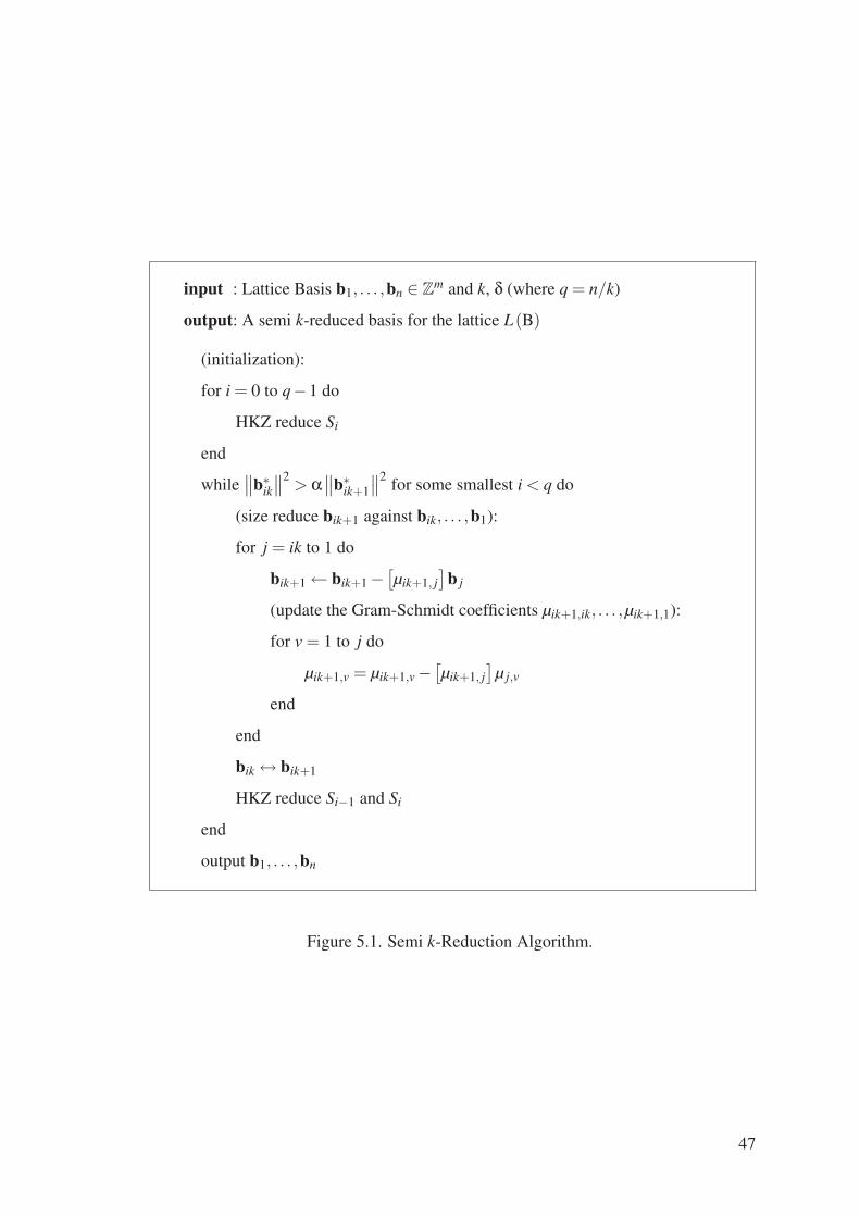
input : Lattice Basis b1, . . . ,bn ∈ Zm and k, δ (where q = n/k)
output: A semi k-reduced basis for the lattice L(B)
(initialization):
for i = 0 to q−1 do
HKZ reduce Si
end
while∥∥b∗ik
∥∥2> α
∥∥b∗ik+1
∥∥2 for some smallest i < q do
(size reduce bik+1 against bik, . . . ,b1):
for j = ik to 1 do
bik+1 ← bik+1−[µik+1, j
]b j
(update the Gram-Schmidt coefficients µik+1,ik, . . . ,µik+1,1):
for v = 1 to j do
µik+1,v = µik+1,v−[µik+1, j
]µ j,v
end
end
bik ↔ bik+1
HKZ reduce Si−1 and Si
end
output b1, . . . ,bn
Figure 5.1. Semi k-Reduction Algorithm.
47

input : Lattice Basis b1, . . . ,bn ∈ Zm and k, δ (where q = n/k)
output: A semi block 2k-reduced basis for the lattice L(B)
(initialization):
for i = 0 to q−1 do
HKZ reduce Si
end
while∥∥b∗ik
∥∥2> α
∥∥b∗ik+1
∥∥2 or δkCi 6 βkkCi+1 for some smallest i < q do
if∥∥b∗ik
∥∥2> α
∥∥b∗ik+1
∥∥2 then
(size reduce bik+1 against bik, . . . ,b1):
for j = ik to 1 do
bik+1 ← bik+1−[µik+1, j
]b j
(update the Gram-Schmidt coefficients µik+1,ik, . . . ,µik+1,1):
for v = 1 to j do
µik+1,v = µik+1,v−[µik+1, j
]µ j,v
end
end
bik ↔ bik+1
HKZ reduce Si−1 and Si
end
if δkCi 6 βkkCi+1 then
HKZ reduce Li−1
end
end
output b1, . . . ,bn
Figure 5.2. Semi Block 2k-Reduction Algorithm.
48

For further information, reader is advised to refer to (Schnorr 1987, Gama, et al. 2006,
Schnorr 2006a).
Remarks on the HKZ reduction:
• An algorithm to perform such HKZ reduction is firstly proposed by Kannan
(1983, 1987b). Later, the algorithm is improved by Helfrich (1985), Schnorr
(1987). Schnorr, in order to perform BKZ reductions, uses his improved version of
Kannan’s algorithm, which is a nn/2+o(n)-time algorithm requiring a polynomial
space. Furthermore, the complexity of Kannan’s algorithm is further refined to
nn/2e+o(n) ≈ n0.184n+o(n) by Hanrot and Stehle (2007). As a side note, Kannan’s
algorithm makes use of the LLL algorithm in order to obtain good bases during
computation.
• There is another algorithm to compute HKZ reduced bases due to Ajtai et al.
(2001) , whose running time is provably bounded by 25.9n by Nguyen and Vidick
(2008). However, there are two drawbacks of this algorithm. It requires an expo-
nential space and there is a tiny probability that the computed basis is not HKZ
reduced, i.e. the algorithm is probabilistic.
• HKZ reduction of the 2k-block πik+1 (bik+1) , . . . ,πik+1 (bik+2k) decreases Di =
∏i−1j=0Ci by at least a factor of δ.
Remarks on the semi reduction algorithms:
• The reduction algorithms form a hierarchy between LLL reduction and HKZ re-
duction. For k = 2 , k-reduction algorithm performs LLL reduction whereas for
k = n the reduction becomes HKZ. In general, the algorithms are called BKZ re-
duction algorithms and semi block 2k-reduction algorithm outputs relatively better
bases while having the same time and space complexity.
• Notice that for k = O(n), the running time gets exponential. Therefore, the algo-
rithms perform HKZ reductions on blocks of size k to avoid an exponential run
time.
Remarks on the complexity and the approximation factors for SVP:
49

• The main difference between the semi k-reduction and the semi block 2k-reduction
is that although they both have the same time and space complexity, the semi k-
reduction produces slightly longer bases. The algorithms are feasible for k 6 25.
• Semi block 2k-reduction requires O(
n2(
kk/2+o(k) +n2)
logB)
arithmetic op-
erations on O(n logB) bit integers and achieves an approximation factor of(6k2)n/(2k).
• For the choice of k = O(logn/ log logn) the approximation factor of semi block
2k-reduction algorithm is 2O(n(log logn)2/ logn) while the run time is still polynomial.
Furthermore, if one uses the probabilistic algorithm in (Ajtai, et al. 2001) within
the blocks of size k, instead of the deterministic SVP algorithm in (Kannan 1987b),
the achieved approximation factor becomes 2O(n(log logn)/ logn) for k = O(logn) in
randomized polynomial time.
• The(6k2)n/(2k) factor is initially given by Schnorr (1987). Furthermore, assuming
the unproven bound γk 6 k/6 for k > 24, one obtains a factor of (k/3)n/k (Schnorr
2001, 2003).
• Ajtai (2003) proves that the best possible approximation factor for the semi block
2k-reduction algorithm is kε(n/k) for some constant ε > 0 under the condition k =
o(n). This implies that if the algorithm runs in polynomial time then we have
already a polynomial time algorithm for finding the shortest nonzero vector.
• Gama et al. (2006) prove the approximation factor of ≈ (βk/δ)(n−1)/(2k). For
k = 24, this factor < (1.165)(n−1)/2, moreover, as noted by (Schnorr 2006a), this
can be shown to be ≈ (1.034)(n−1)/2 under the heuristic in (Schnorr 2003).
5.4. Blockwise Lattice Basis Reduction Variants
5.4.1. BKZ Variants
Schnorr and Euchner (1994) define k-reduced with δ bases by relaxing the con-
ditions of k-reduced bases in another way. A basis b1, . . . ,bn ∈ Zm is k-reduced with δ,
50

1/2 < δ < 1, if it is size reduced and
δ‖b∗i ‖2 6 λ1(πi
(L
(bi, . . . ,bmin{i+k−1,n}
)))2 (5.18)
for i = 1, . . . ,q−1 where q = n/k and 2 < k < n. They propose a practical BKZ variant
which uses LLLFP algorithm proposed by the authors in the same paper. Furthermore,
they show a BKZ reduction algorithm with pruning by presenting a rule to speed up the
enumeration process in the enumeration algorithm. The authors state that the algorithm
has no polynomial time proof however it behaves well in the practice.
Schnorr and Horner (1995) develop a pruning rule based on a particular heuristic
in order to speed up the enumeration of the short lattice vectors. The improvement
yields another BKZ algorithm with pruning, enhancing the enumeration process of the
algorithm presented in (Schnorr and Euchner 1994). The authors state that there is no
polynomial runtime proof for the proposed variant and perform some applications in
order to demonstrate its practicality.
5.4.2. Primal/Dual Segment Reduction
Koy (2004) introduces a basis reduction algorithm which works on k-blocks. The
algorithm is named as the primal/dual segment reduction algorithm, and it runs with the
parameters k,δ in O(
n3kk/2+o(k) +n4)
time, needs to store n2 + O(n) lattice vectors
and obtains the proven approximation factor(αγ2
k
)(n/k−1)/2 where in general α ≈ 4/3
and δ ≈ 1. The algorithm is feasible for k 6 50, and the approximation factor becomes
(k/6)n/k assuming the unproven bound γk 6 k/6 for k > 24. In general, primal/dual
method achieves better approximation factors than the semi block 2k-reduction algo-
rithm, more accurately approximation factor ≈ 1.075(n−1)/2 , for the same blocksize,
since γ2k = Θ(k). However, the semi block 2k-reduction algorithm may become su-
perior if is close to the lower bound βk > k/12 given by Gama et al. (2006) making
βk/δ 6√
αγ2k. Nevertheless, both algorithms perform equally powerful in approxi-
mation of SVP and perform even better (≈ (1.034)(n−1)/2 approximation factor)under
particular heuristic in (Schnorr 2006a). In addition, it is possible to decrease the ap-
proximation factor to ≈ (1.025)(n−1)/2 for k = 80 via replacing the HKZ reduction by
the random sampling reduction in (Schnorr 2003) under the mentioned heuristic. The
resulting algorithm is highly parallel but has no polynomial runtime proof. Also see
51
(Schnorr 2007).
5.4.3. 2k-Block Rankin Reduction and Transference Reduction
Gama et al. (2006) propose a blockwise basis reduction algorithm called 2k-
block Rankin reduction which is an improvement to Schnorr’s semi block 2k-reduction
algorithm. The algorithm make use of the Rankin’s constant, which is the generalization
of the Hermite’s constant, playing a similar role to the Schnorr’s constant βk. However,
this version of the algorithm is only of theoretical interest because it requires a k -Rankin
reduction subroutine which solves the half volume problem exactly and the exact solu-
tion is not known for the dimensions higher than 4. In order to fill this gap, the authors
propose another reduction method which is an approximation algorithm for the half vol-
ume problem in dimension 2k, called the transference reduction. In dimension 2k, it is
cheaper than the 2k-dimensional HKZ reduction used in the semi block 2k-reduction al-
gorithm. The 2k-block Rankin reduction algorithm, when plugged with the transference
reduction, which utilizes an improved reduction strategy while reducing the large blocks
instead of using the HKZ reduction, performs cheaper reductions therefore allows the
use of higher k. The upper bound on the approximation factor ≈ βn/(2k)k 6∼ kn ln2/k is re-
duced by ln2-th power to≈ γn/kk 6∼ kn/k. An important point concerning this discussion is
that the analysis of the Kannan’s shortest vector algorithm by Hanrot and Stehle (2007),
has an effect on the approximation upper bounds of semi block 2k-reduction algorithm
of Schnorr (1987) and the reduction algorithms of Gama et al. (2006) .
5.4.4. Slide Reduction
Gama and Nguyen (2008a) present a polynomial-time blockwise reduction al-
gorithm which finds a short vector within the Mordell’s inequality , γn 6 γ(n−1)/(k−1)k ,
which is the natural generalization of the Hermite’s inequality, γn 6 γ(n−1)2 =
√4/3
(n−1)
achieved by LLL (Lenstra, et al. 1982). The algorithm is called the slide reduction
and achieves (1+ ε)γ(n−k)/(k−1)k ≈ γ(n−k)/(k−1)
k approximation to SVP. This factor is
an improvement of those of (Schnorr 1987, Gama, et al. 2006). However, for k =
O(logn/ log logn), the approximation factor is similar, specifically 2O(n(log logn)2/ logn).
52
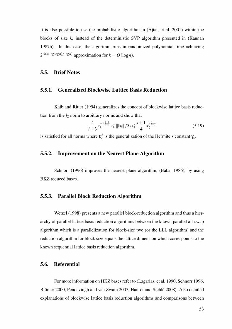
It is also possible to use the probabilistic algorithm in (Ajtai, et al. 2001) within the
blocks of size k, instead of the deterministic SVP algorithm presented in (Kannan
1987b). In this case, the algorithm runs in randomized polynomial time achieving
2O(n(log logn)/ logn) approximation for k = O(logn).
5.5. Brief Notes
5.5.1. Generalized Blockwise Lattice Basis Reduction
Kaib and Ritter (1994) generalizes the concept of blockwise lattice basis reduc-
tion from the l2 norm to arbitrary norms and show that
4i+3
κ−2 i−1
k−1k 6 ‖bi‖/λi 6 i+1
4κ
2 n−1k−1
k (5.19)
is satisfied for all norms where κ2k is the generalization of the Hermite’s constant γk.
5.5.2. Improvement on the Nearest Plane Algorithm
Schnorr (1996) improves the nearest plane algorithm, (Babai 1986), by using
BKZ reduced bases.
5.5.3. Parallel Block Reduction Algorithm
Wetzel (1998) presents a new parallel block-reduction algorithm and thus a hier-
archy of parallel lattice basis reduction algorithms between the known parallel all-swap
algorithm which is a parallelization for block-size two (or the LLL algorithm) and the
reduction algorithm for block size equals the lattice dimension which corresponds to the
known sequential lattice basis reduction algorithm.
5.6. Referential
For more information on HKZ bases refer to (Lagarias, et al. 1990, Schnorr 1996,
Blomer 2000, Pendavingh and van Zwam 2007, Hanrot and Stehle 2008). Also detailed
explanations of blockwise lattice basis reduction algorithms and comparisons between
53

the most practical reduction algorithms can be found in (Gama, et al. 2006, Schnorr
2006a, 2007, Gama and Nguyen 2008a,b).
54
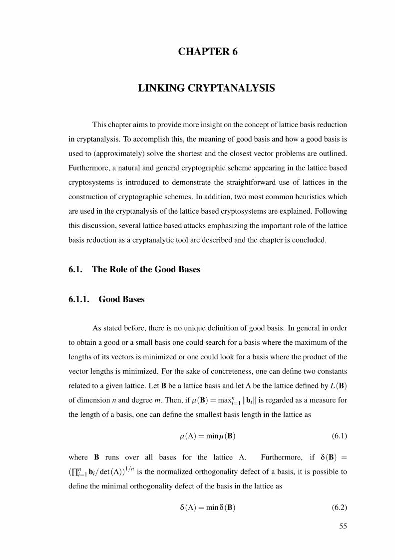
CHAPTER 6
LINKING CRYPTANALYSIS
This chapter aims to provide more insight on the concept of lattice basis reduction
in cryptanalysis. To accomplish this, the meaning of good basis and how a good basis is
used to (approximately) solve the shortest and the closest vector problems are outlined.
Furthermore, a natural and general cryptographic scheme appearing in the lattice based
cryptosystems is introduced to demonstrate the straightforward use of lattices in the
construction of cryptographic schemes. In addition, two most common heuristics which
are used in the cryptanalysis of the lattice based cryptosystems are explained. Following
this discussion, several lattice based attacks emphasizing the important role of the lattice
basis reduction as a cryptanalytic tool are described and the chapter is concluded.
6.1. The Role of the Good Bases
6.1.1. Good Bases
As stated before, there is no unique definition of good basis. In general in order
to obtain a good or a small basis one could search for a basis where the maximum of the
lengths of its vectors is minimized or one could look for a basis where the product of the
vector lengths is minimized. For the sake of concreteness, one can define two constants
related to a given lattice. Let B be a lattice basis and let Λ be the lattice defined by L(B)
of dimension n and degree m. Then, if µ(B) = maxni=1 ‖bi‖ is regarded as a measure for
the length of a basis, one can define the smallest basis length in the lattice as
µ(Λ) = minµ(B) (6.1)
where B runs over all bases for the lattice Λ. Furthermore, if δ(B) =
(∏ni=1 bi/det(Λ))1/n is the normalized orthogonality defect of a basis, it is possible to
define the minimal orthogonality defect of the basis in the lattice as
δ(Λ) = minδ(B) (6.2)
55

here B runs over all bases for the lattice Λ. The search for a good basis requires to find a
basis B where either µ(B) is as close to µ(Λ) as possible or δ(B) is as close to δ(Λ) as
it can get. Furthermore, it is possible to extend the definition of the normalized orthog-
onality defect and the minimal orthogonality defect to the set of n linearly independent
lattice vectors instead of just the basis vectors.
In general, lattice basis reduction algorithms, especially LLL, tend to find more
orthogonal and shorter lattice basis than the given input basis, and as suggested by the
experimental results they perform better than the proven worst cases.
For a more detailed discussion on the lattice problems related to the basis reduc-
tion, see (Micciancio and Goldwasser 2002).
6.1.2. Good Bases and Lattice Problems
In general, to solve the shortest or the closest vector problem, one needs to solve
the more general problem of lattice basis reduction. The importance of the quality of
the lattice basis in the solution of the hard lattice problems such as the shortest and the
closest vector problems can be demonstrated simply as follows.
Let the basis B = {b1,b2} and C = {c1,c2} be the two different bases of the same
lattice as shown in the Figure 6.1. Using the figure, one can immediately note that
• µ(B) < µ(C),
• δ(B) < δ(C).
Considering the shortest vector problem, the basis B yields a better approxima-
tion to the shortest vector problem. In fact, it can be inferred from the figure that B
contains a shortest vector of the lattice. Whereas, the basis C approximates the shortest
vector to within a factor of around ≈ 5.
In order to find the approximate or the exact closest vector to a given target vector,
the fundamental parallelepipeds related to the lattice bases are used. Let B be the any
basis of a given lattice, then the fundamental parallelepiped, or the fundamental domain,
related to the basis B is defined as
F(B) ={
Bx : B ∈ Rm×n,xi ∈ [0,1]}
. (6.3)
56
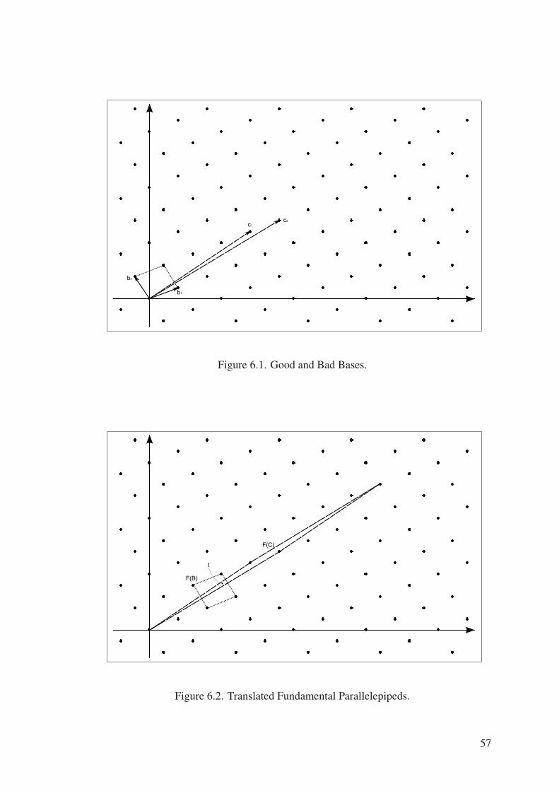
Figure 6.1. Good and Bad Bases.
Figure 6.2. Translated Fundamental Parallelepipeds.
57
Now consider Figure 6.2. Given the target vector t, in order to find the approximate
closest lattice vector to the target vector, the fundamental parallelepipeds related to the
bases B and C are translated to wrap the target vector t. The closest vector is approxi-
mated as the vertex of the translated fundamental parallelepiped which is closest to the
target vector. It is obvious that, for the given target vector in the figure, the close vector
approximated using the lattice basis C is farther than the one approximated using the
basis B. In fact, the latter vector is the closest lattice vector to the given target vector.
6.2. A General Trapdoor Outline
Given a basis for a lattice, it is easy to generate a vector which is close to the
lattice. This can be done by generating a lattice vector using the basis and adding some
carefully chosen vector to obtain a close vector. However, as implied by the closest
vector problem and it variants, to recover the closest lattice vector is not an easy task
using an arbitrary lattice basis. Even the approximations, i.e. the close vectors, are not
sufficient in case the given arbitrary basis is not reduced properly or a good enough basis
can not be found.
For this trapdoor, there are two possibilities to encode the message which can be
stated abstractly as follows. Let v be the generated lattice vector and d be the added vec-
tor which does not belong to the lattice, then a close vector can be obtained as t = v+d.
At this point, one can encode the message inside the lattice vector v or inside the chosen
non lattice vector d which is sometimes called the error vector. In both approaches, ad-
ditional steps are performed to properly, and securely, encrypt the plaintext and decrypt
the ciphertext.
The above scheme is outlined here because it poses a clear and an obvious trap-
door which is easy to understand, reflecting the framework of some of the popular lattice
based cryptosystems such as GGH (Goldreich, et al. 1997) and NTRU (Hoffstein, et al.
1998, 1999). However, the lattice problem on which the GGH cryptosystem is based is
the closest vector problem whereas the NTRU is based on the shortest vector problem
and the closest vector problem. Furthermore, it is important to note that, in general, this
kind of raw trapdoors are not sufficient to built full fledged cryptosystems without taking
further and proper measures to minimize, or if possible remove, the inherent flaws and
58

the decryption errors (if the scheme is probabilistic) etc., while maintaining the perfor-
mance / security trade off at a practical level. These measures are generally composed of
the specific parameters sets and values together with additional and auxiliary function-
ality, which almost always change from one construction to another affecting the overall
system.
It is not necessary to use a similar approach to the one described above in order
to construct a lattice based cryptosystem. For example, Ajtai and Dwork (1997) propose
such a cryptosystem (the AD cryptosystem) which is based on a variant of the shortest
vector problem where the lattice gap λ2/λ1 is polynomial in the dimension. Although
based on a lattice problem, the use of lattices in the AD cryptosystem is not as explicit as
the above scheme. The significance of the AD cryptosystem is that it enjoys an interest-
ing security proof on the worst case hardness of the underlying shortest vector problem
and this type proofs are not present in other lattice based or non lattice based public key
cryptosystems in general.
As a remark, it should be mentioned that the AD and GGH cryptosystems are
broken for all choice of parameter values where the schemes are practical, whereas the
NTRU cryptosystem still remains unbroken after being subject to slight changes over
time.
6.3. Important Heuristics in Practice
6.3.1. Gaussian Heuristic
In a full rank lattice with dimension n, the number of lattice points in the cen-
tered ball of radius r at the origin can be approximated as the number of fundamental
parallelepipeds inside the ball. Thus, the number of such lattice points corresponds to
≈ vol(Bn (0,r))vol(P(B))
(6.4)
This approach is more justifiable if the ball is centered at the origin, the radius grow to
infinity and the dimension (or degree) of the lattice is sufficiently large. If one chooses
the radius so that
vol(P(B)) = det(L(B))≈ vol(Bn (0,r)) (6.5)
59

where, heuristically, it can be deduced there is a non zero lattice point in the ball. There-
fore, the expected length of the shortest vector in the lattice is less than the radius of the
ball. The volume of the n-dimensional ball or radius r is
vol(Bn (0,r))≈(
2πen
)n/2
rn (6.6)
and when the volume of the ball and the lattice are equal,
det(L(B))≈(
2πen
)n/2
rn (6.7)
Solving the approximate equality for the radius r yields
r ≈√
n2πe
det(L(B))1/n (6.8)
Therefore, according to Ajtai (2002), a random full rank lattice Λ satisfies the following
properties based on the Gaussian heuristic with an extremely high probability.
• λ1 = λ1 (Λ) = minv∈Λ−{0}
‖v‖ ≈√ n2πe det(Λ)1/n
• minv∈Λ−{0}
‖v− t‖ ≈√ n2πe det(Λ)1/n where t is a random target vector.
Furthermore, with a high probability, the length of the shortest vector in a lattice lies
between √n
2πedet(Λ)1/n and
√nπe
det(Λ)1/n (6.9)
See (Hoffstein, et al. 1998, Silverman 2006).
6.3.2. Kannan’s Embedding Heuristic
An important strategy in practice to solve the closest vector problem is the Kan-
nan’s embedding method (Kannan 1987b, Nguyen 1999, Micciancio and Goldwasser
2002). The method is not provable in general and therefore may fail to find the closest
vector. It can be used when the target vector is very close to the lattice to find a closest
vector by using an algorithm to solve the (unique) shortest vector problem. The outline
of the method is as follows.
Given a n dimensional and m degree lattice with the basis B = {b1, . . . ,bn},
and a target vector t ∈ Rm, it is possible to embed the n dimensional lattice in Rm to
another lattice with n + 1 dimension in Rm+1. The new lattice is spanned by the basis
60
{(b1,0) , . . . ,(bn,0) ,(t,c)}where the coefficient c is determined depending on the lattice
(in many cases c = 1). Experiments suggest that
• the shortest vector of the new lattice is in the form (t−v,c) where v is a closest
vector to t in the original lattice,
• the second minimum of the new lattice corresponds to the first minimum of the
original lattice,
if the distance to the lattice is smaller than the length of the shortest vector. In fact,
to recover (t−v,c) it is sufficient to approximate the shortest vector problem within a
factor of λ1/‖t−v‖. Also see (Fischlin and Seifert 1999).
6.4. Cryptanalytic Considerations and Lattice Attacks
6.4.1. Brief Considerations
In the lattice based public key cryptosystems, the typical elements which give
rise to the cryptanalytic weaknesses can roughly be listed as follows.
• The structure of the lattice used.
• The choice of systems parameters.
• The key generation, encryption and decryption processes.
• The non-hardness of the underlying problem.
Although listed separately, these issues are closely related to each other. Generally
speaking, there are some certain classes of lattices which seems to be more secure com-
pared to the other classes. The failure in the selection of the appropriate lattice results
in the exploitation of the lattice structure in terms of cryptanalytic attacks. The proper-
ties of the selected lattice are also related to the proper choice of the system parameters
which in almost all cases directly affects the level of security. Furthermore, perhaps more
than the other contemporary public key cryptosystems, the lattice based public key cryp-
tosystems, relies on the properly determined parameters. These parameters have great
impact on the practicality and the security of the system. In addition, being related to the
61

chosen runtime parameters, the flaws in the key generation, encryption and decryption
processes may compromise the security of the cryptosystem seriously. It might be pos-
sible to reduce the hard problem instance used in the process to an easier instance of the
same or another problem, after performing some straightforward computations due to
the flawed mechanism. Another important thing is whether the hardness assumption of
the problem which is used in the construction of the trapdoor is valid or not. For exam-
ple, although a certain problem has hardness proof, it does not mean that all instances of
the problem are equally hard or all the variants of the problem satisfy the same hardness
level or conditions. Therefore, assuming that the underlying problem is hard in case it is
not comes at the expense of practicality, performance and security.
6.4.2. Lattice Attacks
Aside from the general cryptanalytic attacks, there are also lattice attacks on the
lattice based public key cryptosystems, striving to solve approximately or exactly the
underlying lattice problem which is in general the shortest vector problem or the closest
vector problem or a variant of any of them. Although, being different from one lattice
based public key cryptosystem to another, it is possible to describe the lattice attacks
simply as follows.
6.4.2.1. Lattice Attacks on the Private Key
The private key described in the aforementioned scheme is a good basis of the
lattice. It might be possible to recover a good basis by using the reduction algorithms.
However, in general, such approaches are not practical due to the system specifications.
On the other hand, sometimes it is possible to represent the private key as a
short vector in the lattice for practicality. The key still functions as a good lattice basis
however it is just more compact. A similar case arises in NTRU (Hoffstein, et al. 1999).
The underlying problem is the approximate shortest vector problem where the private
key is encoded in a short lattice vector in a lattice which is slightly modified form of
the original. The lattice basis reduction algorithms can be used to recover the private
key after performing some extra computations to minimize the recovery time such as
62
balancing the lattice.
It is important to note that, to obtain some insight on the vulnerability of the
private key, and thus on how the basis reduction algorithms will perform, measuring of
how far a lattice differs from a random lattice is a good approach. In case the private key
is a short vector, the Gaussian heuristic is useful to do this.
6.4.2.2. Lattice Attacks on the Message
It is expected that the vulnerability of message should be close to the vulnerabil-
ity of the private key so that the basis reduction or the lattice attacks will have equally
difficult time and there will be nontrivial exploits.
It might be possible to recover the message by solving the closest vector problem
with some proper measures. In general, the cryptosystems are specified in a such way
that exactly solving the underlying problem (at least directly) is highly impractical and
requires extensive computation. At this point, the reduction algorithms come handy. It
might be possible to combine the inherent flaws in the encryption process with the Kan-
nan’s embedding heuristic outlined before and solve the shortest vector approximately
and retrieve the close lattice vector where the message is encoded. This is the way how
Nguyen (1999) breaks the GGH cryptosystems in its original form in (Goldreich, et al.
1997), using two weaknesses related to the encryption process where the first one is the
relatively short length of the error vectors compared to the lattice vectors and the other
is the flawed way of choosing the entries of the error vectors. The first weakness causes
the basis reduction algorithms to be applied practically to recover the close vector and
the second one allows the simplification in the underlying closest vector problem. Al-
though, according to the practical behaviour of the reduction algorithm used, it might be
possible to break the cryptosystem even if no serious flaws are existent.
In the NTRU cryptosystem, a similar situation to the one described in recovering
the NTRU private key arises. The message vector can be encoded in a short lattice vector
in a slightly different lattice and lattice basis reduction algorithms can be applied to solve
the approximate shortest vector problem.
63

6.4.2.3. Lattice Attacks on a Spurious Key
This approach is firstly proposed for the cryptanalysis of the NTRU cryptosystem
in (Coppersmith and Shamir 1997). It requires finding a sufficiently short vector which
will as the private key during the decryption rather than finding the private key itself. In
particular, it can be possible to find several vectors (not as short as the private key) which
can be used to decrypt the message partially. Then, these partial decryptions are pieced
together to get the full decryption. This approach is practical if the time required to find
the spurious key is significantly less than the time required to find the private key.
6.4.2.4. An Example of Exploiting the Lattice Structure
May (1999) exploits the structure of the special class of lattices used in the NTRU
cryptosystem and proposes a lattice based attack. The attack aims to make the lattice gap
as big as possible so that heuristically the approximation to the shortest vector within a
factor will yield the shortest vector itself, i.e. the private key. To do this, another class of
lattices, which have reduced dimension and satisfy some certain conditions, are inferred
from the Coppersmith-Shamir lattices, see (Coppersmith and Shamir 1997, Hoffstein,
et al. 1999). Furthermore, the generalization of this approach is also discussed in (May
and Silverman 2001).
Note that the discussed attacks are in general tightly related to the structure of the
particular cryptosystems. However, in all attacks, the lattice basis reduction algorithms
play crucial role together with some certain heuristics. Furthermore, it might also be pos-
sible to improve the general cryptanalytic attacks, such as the chosen ciphertext attacks,
the partial information attacks and the brute force attacks, using the lattice algorithms
depending on the chosen lattice based public key cryptosystem.
6.5. Referential
For more information on lattice based cryptography and improvements refer to
(Ajtai and Dwork 1997, Dwork 1998, Goldreich, et al. 1997, Hoffstein, et al. 1999,
Cai and Cusick 1999, Sakurai 2000, Micciancio 1999, 2001a, Regev 2004b, 2005, Ajtai
64

2005, Paeng, et al. 2002, Kawachi, et al. 2007, Peikert and Waters 2007, Gentry, et al.
2007, Micciancio 2007). The cryptanalysis of and lattice based attacks on the various lat-
tice based cryptographic constructions can be found in (Coppersmith and Shamir 1997,
Nguyen and Stern 1998, May 1999, Nguyen 1999, Gentry 2001, Gentry and Szydlo
2002, Nguyen and Regev 2006, Han, et al. 2007). Furthermore, lattices are important
tools for the cryptanalysis of non lattice based constructions and details can be found in
(Joux and Stern 1998, Nguyen 2001, Micciancio 2002, Nguyen 2008). As a last note,
reader should refer to (Gama and Nguyen 2008b) for significant assessments on how
lattice basis reduction methods behave in practice arousing security and efficiency im-
plications on the cryptanalytic and cryptographic perspectives.
65

CHAPTER 7
AN EVALUATION FOR EXPERIMENTS
As mentioned before, the lattice basis reduction algorithms, in practice, perform
much better than the expected (and proved) worst case bounds in terms of running time
and output quality. This phenomenon affects the understanding of the current concepts
of the basis reduction and the reduction algorithms, and shows that more insight should
gained on what is really going on behind these algorithms. The aim of this section is to
provide practical assessments on the most popular variants of the LLL and BKZ lattice
basis reduction algorithms. To do this, the works of Nguyen and Stehle (2006), Gama
and Nguyen (2008b) are exploited.
7.1. Importance of the Practical Assessments
Assessments of the practical performance of the lattice basis reduction algo-
rithms are necessary and important for many reasons. Some of these reasons can be
stated as follows.
• Although experimental, it has been a fact that the lattice basis reduction algorithms
perform much better in practice.
• The use of various heuristics in different algorithmic variants brings forth the ne-
cessity of the experimental measurements.
• New heuristics, which can be used to further speed up the reduction process, may
be revealed, playing a role in the proposition of new reduction schemes.
• The experimental measurements and observations may reveal new information on
the practical hardness of the main lattice problems and enable the comparison of
the various computational hardness assumptions used in theoretical lattice-based
cryptography.
• The observations may also reveal some classification among different lattice
66

classes, such as hard and easy lattice instances. Thus, several adjustments can
be performed on the choice of parameters in the cryptographic schemes in order
to strengthen the security level of the instance.
• The practical assessments are likely to allow discovery of the differences and sim-
ilarities between the practical and the theoretical behaviour of the reduction algo-
rithms.
• The assessments can be used to draw the limits on what is achievable by the use
of today’s algorithms.
Furthermore, it is important to note that the most commonly used reduction al-
gorithms in practice are not the classical version of the LLL algorithm (Lenstra, et al.
1982) and the BKZ algorithm (Schnorr 1987). Instead, the use of variants of these
algorithms proposed in (Schnorr and Euchner 1994) are still preferred widely by crypt-
analysts and mathemticians etc, because these algorithms have managed to uphold their
practical superiority against the many other heuristic and theoretic variants which have
been introduced since then.
7.2. Preliminary Remarks
Nguyen and Stehle (2006) are the firsts to give a detailed and clearer explanation
on the average case behaviour of the LLL reduction algorithm by performing extensive
experiments and proposing heuristic arguments assessing the practicality of the algo-
rithm (and some of its variants). Furthermore, Gama and Nguyen (2008b) extend the
study to the most popular reduction algorithms in the practice, namely LLL (Lenstra,
et al. 1982), LLL with deep insertions (Schnorr and Euchner 1994) and BKZ variant in
(Schnorr and Euchner 1994). The authors discover very important experimental results
on the limits of what today’s most practical reduction algorithms can achieve. Shortly,
they show that the lattice basis reduction algorithms are very optimistic in practice and
state that the current algorithms, achieve the approximation factor of 6 1.01n on the aver-
age and 6 1.02n in the worst case. Furthermore, it is concluded that to prevent reduction
algorithms to take advantage of the lattice structure of the worst cases, dimension should
be very high.
67

In order to perform solid experiments, one needs to use mathematically sound
concept of randomness in lattices. Such concepts are also discussed and utilized in
(Nguyen and Stehle 2006, Gama and Nguyen 2008b), and will shortly be introduced
here.
The concept of random lattices is a mathematically sophisticated subject. As
stated by Nguyen and Stehle (2006), one might select a randomly generated lattice which
is used in a particular application such as algorithmic number theory or cryptography.
However, it should be noted that this type of lattices may not be random in the math-
ematical sense. For example, in cryptanalysis, lattices to which reduction algorithms
are applied generally have their first minimum much shorter than all the other minima.
Nevertheless, it can be beneficial to restrict the selection of lattices from a particular
class to discuss the practicality of the reduction algorithms in the problems where the
chosen particular subset is significant. Ajtai (2002), Goldstein and Mayer (2003) pro-
vide efficient means to generate lattices in a mathematically random sense. The random
lattices satisfy the following approximate equality based on the Gaussian heuristic with
an extremely high probability,
λ1 (L)
vol (L)1/n≈ Γ(1+n/2)1/n
√π
≈√
n2πe
. (7.1)
Once a lattice is selected, one needs to choose a lattice basis out of infinitely
many possible choices in random. In this case, however, there is no clear definition of
a random basis. It may be expected that the random basis consists of long vectors and
is not reduced. As a random basis, one might use the Hermite normal form (HNF) of
the lattice since it gives relatively less information on the lattice and can be computed in
polynomial time. However, HNF of some lattices may have some special properties (for
example, the HNF of NTRU lattices (Hoffstein, et al. 1998) are reduced in some sense).
Another option could be to use the heuristic approach of Goldreich et al. (1997) which is
the transformation of the secret basis into an equivalent large public basis by randomly
multiplying with the generators of special linear group over the set of integers, i.e. the
set of integer matrices with determinant 1. Unfortunately, in this approach, it is difficult
to control the size of the entries and theoretical results are hard to obtain. On the other
hand, a promising and less heuristic approach is presented in (Nguyen and Stehle 2006).
The approach considers the full-dimensional integer lattices. If the norm bound of the
basis is much greater than the n-th root of the lattice determinant, i.e. B >> (detΛ)1/n,
68

it is possible to sample efficiently and uniformly lattice points whose norms are bounded
by B. (Ajtai 1996) (Klein (2000) also proposes a sound way to sample lattice vectors,
see also (Gentry, et al. 2007, Nguyen and Vidick 2008)). The sampled points are linearly
independent with an extremely high probability, however they do not necessarily form a
basis for the lattice. To lift this set of linearly independent vector to a lattice basis, (Ajtai
1996) or lemma 7.1 of (Micciancio and Goldwasser 2002) can be used. The produced
basis has the norm bound (√
n/2)B.
Another important notion is the random reduced basis. Nguyen and Stehle (2006)
discuss different concepts of random LLL reduced bases. It seems convenient to adapt
their practical definition. The procedure is to choose a random lattice and select a random
basis, and then apply the decided reduction algorithm to obtain the reduced basis. In
mathematical sense, the reduced basis may not be random. The selection of a random
basis is crucial, since it affects the outcome and the resulting distribution. If an already
reduced basis is selected as a random basis, the output will be atypical.
7.3. Experimental Details
The main purpose of the remaining sections is to perform experiments on the
most popular variants of the LLL and BKZ lattice basis reduction algorithms in order to
observe the effects of the common parameter on the their practical behaviour in terms of
running time and the achieved SVP approximation factor constant. To do this:
• Random knapsack lattices are used. The basis vectors are selected as the rows of
the randomly generated n× (n+1) matrices of the form
b1
b2...
bn
=
k1 1 0 . . . 0
k2 0 1 . . . 0... 0 0 . . . 0
kn 0 0 . . . 1
(7.2)
where ‖bi‖6 B for i = 1, . . . ,n.
• The size parameter logB is kept fixed, logB≈ 128 bits.
• Gaussian heuristic is used to calculate the SVP approximation factor constant,
69

which is defined as
a =( ‖b1‖
λ1 (L)
)1/n
≈(
‖b1‖vol (L)1/n
√2πen
)1/n
(7.3)
Furthermore, the following libraries are benefited from in order to perform the
mentioned tasks.
• NTL 1 version 5.4.2 is used to perform experiments on variants of the most prac-
tical the lattice basis reduction algorithms, namely LLL XD, LLL XD with deep
insertions (LLL XD DEEP) and BKZ XD which uses Gram-Schmidt orthogonal-
ization and extended exponent doubles (see the library documentation).
• FPLLL 2 version 2.1.6 is used for random lattice basis generation. However, the
basis generation code is slightly modified and extended for the process.
• GMP 3 version 4.2.2 and MPFR4 version 2.3.1 are used for the underlying big
integer and floating point number arithmetic.
As for the experimentation environment, a personal computer with P4 (Dual
Core) 1.8Ghz 64 bit CPU, 1 GB RAM and Fedora Core 7 operating system is used.
The obtained results are collectively given in Chapter 8 as conclusions.
1NTL, NTL: A Library for doing Number Theory, http://www.shoup.net/ntl/ (accessed May 5, 2008)2FPLLL, The FPLLL Library, http://perso.ens-lyon.fr/damien.stehle/english.html#software (accessed
May 18, 2008)3GMP, GNU MP: The GNU Multiple Precision Arithmetic Library, http://gmplib.org/ (accessed May
20, 2008)4MPFR, The Multiple Precision Floating-Point Reliable Library, http://www.mpfr.org/ (accessed May
20, 2008)
70
CHAPTER 8
CONCLUSION
In this chapter, the experimental results are demonstrated considering the re-
marks made in the previous chapter. Furthermore, some comments are provided regard-
ing the complementary studies which can be performed in the future.
8.1. Observations and Results
This section presents the results of the experiments which are performed by se-
lecting the delta parameter among the set of values {0.5,0.51,0.6,0.7,0.8,0.9,0.99}.
Furthermore, during the experiments
• The deep parameter of the LLL with deep insertion algorithm is ranged from 10
to 50 in increments of 10.
• The blocksize parameter of the BKZ algorithm is varied from 10 to 30 in incre-
ments of 5.
• The dimension parameter n is ranged from 50 to 300 in increments of 50 in case
of LLL and LLL with deep insertion algorithms, and from 50 to 100 in increments
of 10 in case of BKZ algorithm.
8.1.1. LLL XD
The running times and approximation factor constants achieved by LLL XD are
given in Figures A.1 and A.2 respectively.
The running time of LLL XD can be bounded by a polynomial function in n.
This can be derived from Figure A.1(a). The log time values, i.e. the timings plotted
in logarithmic scale, in the figure have decreasing slopes, which implies a polynomial
runtime in n. Furthermore, Figure A.1(b) shows that, although the running time seems
to be exponential in delta when the logarithmic plot is examined, in practice, the effect
71

of delta on the running time of LLL XD is relatively less significant especially when n
gets larger since the speed up values for decreasing delta are greater in lower n values.
The SVP approximation factor constants achieved by LLL XD are given in Fig-
ure A.2. For fixed delta, a values seem to converge to as n increases. In addition, as
shown in Figure A.2(b), a values decrease as with increasing delta for fixed n. The dif-
ference between achieved a values for high and low n (delta) is remarkable and these
values get closer as delta (n) increases. One may find the decline in the approximation
factor constants unexpected, however it has a straightforward explanation. In case of
fixed n, the value of a is directly controlled by ‖b1‖, and ‖b1‖ decreases as delta in-
creases. On the other hand, when delta is fixed, the value of a is mainly controlled by
n. Since size parameter logB is fixed, ‖b1‖ has no apparent monotonic behaviour, and,
in general, the increasing effect of the vol (L)1/n is slightly dominated by the decreasing
effect of√
n Even if the value of an =(‖b1‖/vol (L)1/n √
2πe/n)
tends to increase, this
increase is not sufficient to overcome the effect of taking the n-th root.
8.1.2. LLL XD DEEP
Figures B.1 through B.6 summarize the main parameters and their effect on the
runtime of LLL XD with deep insertions (or shortly LLL XD DEEP).
Figures B.1 and B.2 show that the running time of LLL XD DEEP is polynomial
in n since the slopes of log graphs in the figure have decreasing tendencies. One might
note that, in higher n, the curves in the figure tend to be linear, which is also more appar-
ent when delta is higher. Nevertheless, this is not sufficient to state that the running time
is be exponential or super-polynomial. Therefore, further experiments can be performed
by increasing n in smaller increments in order to draw stronger conclusions.
The previous literature, such as (Gama and Nguyen 2008b), on the subject states
that LLL XD DEEP has running time exponential in deep. However, according to the
observations shown in Figures B.3 and B.4, the running time can be bounded by a poly-
nomial function in deep for random knapsack lattices. In addition, it can be noted that
when n gets larger, the shape of the timing curves becomes more similar to those of the
exponential curves. This is more apparent for high delta. These arguments arouse the
question whether the knapsack lattices are easier to reduce on the average.
72

The effect of delta on the runtime can better be observed in the graphs in Figures
B.5 and B.6. It is shown that, for fixed fixed deep and n, the runtime of LLL XD DEEP
seem to be O(−1/ log(delta)). The graphs show that a take-off seems to occur after
around delta = 0.90, and it is more apparent and sharper for larger deep and/or n values.
Further experiments yield the fact that this take-off generally occurs around delta≈ 0.96.
The SVP approximation factor constants, a values, achieved by LLL XD DEEP
with respect to the parameters n, deep and delta are give in Figures B.7 through B.12.
Figures B.7 and B.8 show that the achieved approximation factor constants de-
crease and slowly converge to 1 as n increases. However, it should be noted that there
is a frequently observed exceptional circumstance when n is sufficiently low. In the ex-
periments, it is observed that, LLL XD DEEP for n = 50 achieves better a, than those
achieved by higher n for almost all fixed deep and delta values . The achieved constants
may even beat those of n = 300. This can be justified as follows. As n increases, an
increases as usual. However, since an values are already very low for sufficiently small n
such as n = 50, the effect of taking 1/n-th power does not suffice to obtain lower a values
for bigger n than those of sufficiently small n. Thus, for such small n, lower a values
are calculated. This occurrence is more visible when deep becomes larger. However, as
deep increases, one needs higher delta to beat larger n. On the other hand, for n > 100,
the steady decrease in a values can be explained as in the discussion for LLL XD in the
previous section.
The SVP approximation factor constants are also noted to be convergent with
deep as implied by Figures B.9 and B.10. Unlike they do with respect to n, a values
converge relatively faster with respect to deep. It can bee seen from the figure that,
for fixed n and delta, increasing deep value after some certain point may not help to
improve the achieved approximation factor constants practically. If existent, this certain
point varies according to the chosen n and delta, and it seems to inrease for higher values
of n and delta.
As for the effect of delta on the achieved a values, Figures B.11 and B.12 can
provide some insight. Obviously, if one increases delta, smaller a values are obtained.
Furthermore, the decreasing a curves seem to be linear except for n = 50, which is
already discussed above in this section.
Considering the discussion made so far, the following remarks hints on the pos-
73

sible means to exploit the results of the experiments.
• Instead of using high end delta values, one may choose to relax delta and increase
the value of deep parameter to possibly achieve approximation factor constants
which are as good or slightly worse. However, in this process, it is important to
keep in mind that raising delta beyond ≈ 0.96 greatly increases the running time,
and increasing deep beyond some certain point may not improve the achieved a
values, while causing a possible decline in the runtime performance.
• Another way to achieve better results is to increase the dimension of the lattice. If
one can devise a way to efficiently embed a given low dimensional lattice to that
of high dimension, it might be possible to obtain better approximation factor con-
stants. The crucial point is that, during the embedding process, particular lattice
properties, such as the value of the size parameter and the type of the lattice etc.,
should remain unchanged, although it might be possible to tolerate slight changes.
• It is important to note that it might be possible to combine the remarks made above.
While performing these kind of attempts to increase the runtime performance or
the achieved approximation factor constants, one should carefully choose the pa-
rameter values after measuring the trade-offs and thoroughly analyzing the prob-
lem at hand so that unexpected outcomes can be avoided.
8.1.3. BKZ XD
The running time of BKZ XD with respect to n, blocksize and delta parameters
are shown in Figures C.1 through C.6.
It is shown in Figures C.1 and C.2 that the running time of BKZ XD is poly-
nomial in n when blocksize parameter is low, such as blocksize < 20. However, as
it is further increased, running time for low and high end delta values begin to get
super-polynomial. It can be seen that for blocksize > 20, BKZ XD is exponential
in n for delta = 0.5, and for blocksize = 30, BKZ XD is exponential for delta =
0.5,0.6,0.99. One should also note that no measurements are taken for delta = 0.5,0.6
when blocksize = 30. This implies that BKZ XD is highly impractical for small when
blocksize is high.
74
Running time of BKZ XD seem to be super-exponential in blocksize for all val-
ues used in the experiments. When Figures C.3 and C.4 are examined, it can be observed
that there is a sudden increase in the running time after blocksize ≈ 20. For low end
delta values, such as 0.5 and 0.6, the increase is more apparent and occurs at relatively
smaller blocksize values. In addition, for larger n, the increase for high end delta val-
ues, such as 0.99, also shows significant growth. One can also derive that BKZ XD for
blocksize > 30 is highly impractical for low and high end delta values in high dimen-
sions.
Figures C.5 and C.6 show the effect of delta in the running time of BKZ XD.
It is clear that as delta gets closer to 1, the running time increases. For moderate and
large values of blocksize, the running time seems to be O(−1/ log(delta)) when delta is
sufficiently large. Moreover, though it has already been mentioned, one can more clearly
observe that low and high end delta values cause a significant increase in the running
time as blocksize values get larger or in higher n. Therefore, it is natural to state that
BKZ XD might still be practical for higher blocksize values such as blocksize > 30 in
relatively higher dimensions, if delta values are chosen moderately.
As for the achieved SVP approximation factor constants, Figures C.7 through
C.12 provide some insight.
In the experiments, no general pattern emerges concerning the behaviour of
achieved a values with respect to the parameter n. However, it is observed relaxation
of delta causes apparent fluctuations and the a vs. n curves seem to be relatively more
stable, and increasing proportional to n, for larger values of delta. It is noted that more
experiments are likely to smoothen the curves, which turn out to be linear, for moder-
ate and large values of delta. Furthermore, the cause of the increase in the achieved
constants can be stated as follows. Due to the nature of BKZ XD, the growth of the
calculated an =(‖b1‖/vol (L)1/n √
2πe/n)
values is high enough that taking the n-th
root to obtain the SVP approximation factor constants is not sufficient to cause a decline
with the increasing n. As usual, selecting logB to be fixed and using knapsack lattices
(may) all have certain effects on this occurrence.
The effect of blocksize parameter on a is given in Figures C.9 and C.10. Since
the blocksize controls the quality of the computed bases, the value of a decreases with
the increasing blocksize. This directly leads to decreasing curves in the figure. As in the
75
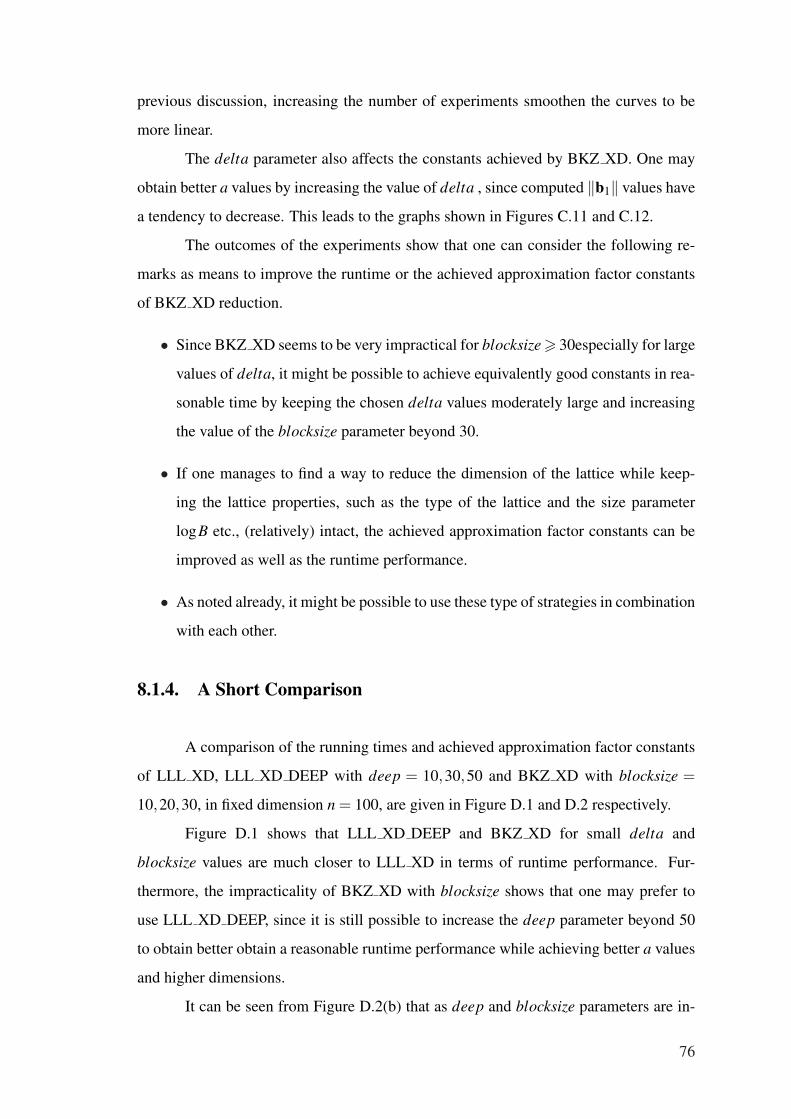
previous discussion, increasing the number of experiments smoothen the curves to be
more linear.
The delta parameter also affects the constants achieved by BKZ XD. One may
obtain better a values by increasing the value of delta , since computed ‖b1‖ values have
a tendency to decrease. This leads to the graphs shown in Figures C.11 and C.12.
The outcomes of the experiments show that one can consider the following re-
marks as means to improve the runtime or the achieved approximation factor constants
of BKZ XD reduction.
• Since BKZ XD seems to be very impractical for blocksize > 30especially for large
values of delta, it might be possible to achieve equivalently good constants in rea-
sonable time by keeping the chosen delta values moderately large and increasing
the value of the blocksize parameter beyond 30.
• If one manages to find a way to reduce the dimension of the lattice while keep-
ing the lattice properties, such as the type of the lattice and the size parameter
logB etc., (relatively) intact, the achieved approximation factor constants can be
improved as well as the runtime performance.
• As noted already, it might be possible to use these type of strategies in combination
with each other.
8.1.4. A Short Comparison
A comparison of the running times and achieved approximation factor constants
of LLL XD, LLL XD DEEP with deep = 10,30,50 and BKZ XD with blocksize =
10,20,30, in fixed dimension n = 100, are given in Figure D.1 and D.2 respectively.
Figure D.1 shows that LLL XD DEEP and BKZ XD for small delta and
blocksize values are much closer to LLL XD in terms of runtime performance. Fur-
thermore, the impracticality of BKZ XD with blocksize shows that one may prefer to
use LLL XD DEEP, since it is still possible to increase the deep parameter beyond 50
to obtain better obtain a reasonable runtime performance while achieving better a values
and higher dimensions.
It can be seen from Figure D.2(b) that as deep and blocksize parameters are in-
76

creased, both LLL XD DEEP and BKZ XD achieve similar approximation factor con-
stants. This gives even more reason to prefer LLL XD DEEP over BKZ XD. However,
one should keep in mind the reduction strategies noted in the previous sections, which
include the relaxation of delta values and increasing deep and blocksize parameters for
LLL XD DEEP and BKZ XD respectively, can still be useful to increase the perfor-
mance of both reduction mechanisms.
8.2. Future Studies
Throughout this study, the most famous lattice basis reduction algorithms are ex-
amined in terms of theoretical and practical perspectives while considering their crypt-
analytical aspects. The results of the experiments demonstrated in the previous section
yield some preliminary practical assessments on the effects of the common delta pa-
rameter on the most famous and efficient variants of the LLL and BKZ basis reduction
algorithms. It should be noted that, the experiments are performed upon random knap-
sack lattices where logB is fixed and the outcomes arouse a couple of questions.
First, it might be convenient to find out whether the decrease in the achieved
approximation factor constants for LLL XD and LLL XD DEEP as the dimension of
the lattices increases stems only from the fact that logB is fixed and the lattice are of
knapsack type. It might be fruitful to research whether there are other types of lattices
which display similar behaviour or whether this occurrence is exploitable in any other
way.
Next, it is noted that in sufficiently low dimensions the approximation factor con-
stants achieved by LLL XD DEEP surpasses some of the constants achieved in higher
dimensions. It is possible that this happens due to the fact that, with respect to the
chosen values, the lattice dimension n is too low and thus unexpectedly good values
are obtained. Nevertheless, before coming to a strict conclusion, one should investigate
whether this experimental occurrence is recurring in much higher dimensions or in other
type of lattices.
Also, the runtime behaviour of LLL XD DEEP on random knapsack lattices
points out that the knapsack lattices may be easier to reduce on the average with re-
spect to other types of lattices. It might be useful to classify the lattices in such a way
77

that different reduction strategies can be followed for different lattice classes.
Finally, the experiments show that the effect of delta on the runtime performance
and the output quality of the algorithms, especially LLL XD DEEP and BKZ XD, is
significant. When careful measures are taken, these algorithms may yield better results
running with even higher deep and blocksize parameters in higher dimensions.
In the light of the above remarks, it seems to be useful to extend the discussion
to other types of lattices and perhaps to also investigate the distribution of ‖b1‖ and
vol (L)1/n values and the Gram-Schmidt coefficients etc. in order to obtain better idea on
the output quality of the considered algorithms. The possible criterion and background
which might be helpful to perform such a research can be found in (Backes and Wetzel
2002, Nguyen and Stehle 2006, Gama and Nguyen 2008b).
78

REFERENCES
Aardal, K. I. 1999. Lattice basis reduction and integer programming. Technical Report
UU-CS-1999-37, Utrecht University.
Agrell, E., T. Eriksson, A. Vardy, and K. Zeger. 2002. Closest point search in lattices.
IEEE Transactions on Information Theory 48(8): 2201–2214.
Aharonov, D. and O. Regev. 2003. A lattice problem in quantum NP. FOCS ’03:
Proceedings of the 44th Annual IEEE Symposium on Foundations of Computer
Science 210–219.
Aharonov, D. and O. Regev. 2005. Lattice problems in NP ∩ coNP. Journal of the
ACM 52(5): 749–765.
Ajtai, M. 1996. Generating hard instances of lattice problems (extended abstract). STOC
’96: Proceedings of the 28th Annual ACM Symposium on Theory of Computing
99–108.
Ajtai, M. 1998. The shortest vector problem in l2 is NP-hard for randomized reductions
(extended abstract). STOC ’98: Proceedings of the 30th Annual ACM Symposium
on Theory of Computing 10–19.
Ajtai, M. 2002. Random lattices and a conjectured 0 - 1 law about their polynomial
time computable properties. FOCS ’02: Proceedings of the 43rd Annual IEEE
Symposium on Foundations of Computer Science 733–742.
Ajtai, M. 2003. The worst-case behavior of schnorr’s algorithm approximating the short-
est nonzero vector in a lattice. STOC ’03: Proceedings of the 35th Annual ACM
Symposium on Theory of Computing 396–406.
Ajtai, M. 2005. Representing hard lattices with o(n log n) bits. STOC ’05: Proceedings
of the 37th Annual ACM Symposium on Theory of Computing 94–103.
Ajtai, M. and C. Dwork. 1997. A public-key cryptosystem with worst-case/average-case
equivalence. STOC ’97: Proceedings of the 29th Annual ACM Symposium on
Theory of Computing 284–293.
79

Ajtai, M., R. Kumar, and D. Sivakumar. 2001. A sieve algorithm for the shortest lattice
vector problem. STOC ’01: Proceedings of the 33rd Annual ACM Symposium on
Theory of Computing 601–610.
Ajtai, M., R. Kumar, and D. Sivakumar. 2002. Sampling short lattice vectors and the
closest lattice vector problem. COCO ’02: Proceedings of the 17th Annual IEEE
Conference on Computational Complexity 41–45.
Akhavi, A. 2002. Random lattices, threshold phenomena and efficient reduction algo-
rithms. Theoretical Computer Science 287(2): 359–385.
Akhavi, A. 2003. The optimal LLL algorithm is still polynomial in fixed dimension.
Theoretical Computer Science 297(1-3): 3–23.
Akhavi, A. and D. Stehle. 2008. Speeding-up lattice reduction with random projections
(extended abstract). LATIN 2008: Theoretical Informatics 4957/2008 of Lecture
Notes in Computer Science 293–305.
Arora, S., L. Babai, J. Stern, and Z. Sweedyk. 1997. The hardness of approximate
optima in lattices, codes, and systems of linear equations. Journal of Computer
and System Sciences 54(2): 317–331.
Babai, L. 1986. On Lovasz’ lattice reduction and the nearest lattice point problem.
Combinatorica 6(1): 1–13.
Backes, W. and S. Wetzel. 2001. Lattice basis reduction with dynamic approximation.
WAE ’00: Proceedings of the 4th International Workshop on Algorithm Engineer-
ing 1982/2001: 63–73.
Backes, W. and S. Wetzel. 2002. Heuristics on lattice basis reduction in practice. Journal
of Experimental Algorithmics 7 1–21.
Banaszczyk, W. 1993. New bounds in some transference theorems in the geometry of
numbers. Mathematische Annalen 296(1): 625–635.
Blomer, J. 2000. Closest vectors, successive minima, and dual HKZ-Bases of lattices.
Automata, Languages and Programming 1853/2000: 248–259.
80

Blomer, J. and S. Naewe. 2007. Sampling methods for shortest vectors, closest vectors
and successive minima. Automata, Languages and Programming 4596/2007: 65–
77.
Blomer, J. and J.-P. Seifert. 1999. On the complexity of computing short linearly inde-
pendent vectors and short bases in a lattice. STOC ’99: Proceedings of the 31st
Annual ACM Symposium on Theory of Computing 711–720.
Buchmann, J. and V. Kessler. 1990. Computing a reduced lattice basis from a generating
system with applications.
Buchmann, J. and C. Ludwig. 2006. Practical lattice basis sampling reduction. Algo-
rithmic Number Theory 4076/2006: 222–237.
Cai, J.-Y. 1998. A relation of primal-dual lattices and the complexity of shortest lattice
vector problem. Theoretical Computer Science 207(1): 105–116.
Cai, J.-Y. 1999. Some recent progress on the complexity of lattice problems. COCO ’99:
Proceedings of the 14th Annual IEEE Conference on Computational Complexity
158–178.
Cai, J.-Y. 2000. The complexity of some lattice problems. Algorithmic Number Theory
1838/2000: 1–32.
Cai, J.-Y. 2001. On the average-case hardness of CVP. FOCS ’01: Proceedings of the
42nd IEEE Symposium on Foundations of Computer Science 308–317.
Cai, J.-Y. and T. W. Cusick. 1999. A lattice-based public-key cryptosystem. Information
and Computation 151(1-2): 17–31.
Cai, J.-Y. and A. Nerurkar. 1997. An improved worst-case to average-case connection
for lattice problems. FOCS ’97: Proceedings of the 38th Annual IEEE Symposium
on Foundations of Computer Science 468–477.
Cai, J.-Y. and A. Nerurkar. 1999. Approximating the SVP to within a factor 1+1/dimε
is NP-Hard under randomized reductions. Journal of Computer and System Sci-
ences 59(2): 221–239.
81

Cai, J.-Y. and A. Nerurkar. 2000. A note on the non-NP-hardness of approximate lattice
problems under general Cook reductions. Information Processing Letters 76(1-2):
61–66.
Cassels, J. 1997. An introduction to the geometry of numbers. Berlin: Springer-Verlag.
Chen, W. and J. Meng. 2006. The hardness of the closest vector problem with prepro-
cessing over l∞ norm. IEEE Transactions on Information Theory 52(10): 4603–
4606.
Coppel, W. A. 2006. The geometry of numbers. In Number theory, 385–426. Springer
US.
Coppersmith, D. and A. Shamir. 1997. Lattice attacks on NTRU. Advances in Cryptol-
ogy - EUROCRYPT ’97 1233/1997: 52–61.
Daude, H. and B. Vallee. 1994. An upper bound on the average number of iterations of
the LLL algorithm. Theoretical Computer Science 123(1): 95–115.
Dinur, I. 2000. Approximating SVP∞ within almost-polynomial factors is NP-Hard.
Algorithms and Complexity 1767/2000: 263–276.
Dinur, I. 2002. Approximating SVP∞ to within almost-polynomial factors is NP-hard.
Theoretical Computer Science 285(1): 55–71.
Dinur, I., G. Kindler, R. Raz, and S. Safra. 2003. Approximating CVP to within almost-
polynomial factors is NP-Hard. Combinatorica 23(2): 205–243.
Dinur, I., G. Kindler, and S. Safra. 1998. Approximating-CVP to within almost-
polynomial factors is NP-hard. FOCS ’98: Proceedings of the 39th Annual IEEE
Symposium on Foundations of Computer Science 99–109.
Dwork, C. 1998. Lattices and their application to cryptography. University of Cal-
ifornia. http://www.math.ucdavis.edu/ %7Edeloera/misc/mathresearch/interesting
papers/Dwork/gitter.ps (accessed at April 14, 2008).
Fischlin, R. and J.-P. Seifert. 1999. Tensor-based trapdoors for CVP and their applica-
tion to public key cryptography (extended abstract). Cryptography and Coding
1746/1999: 801–814.
82

Furst, M. L. and R. Kannan. 1989. Succinct certificates for almost all subset sum prob-
lems. SIAM Journal on Computing 18(3): 550–558.
Gama, N., N. Howgrave-Graham, H. Koy, and P. Q. Nguyen. 2006. Rankin’s con-
stant and blockwise lattice reduction. Advances in Cryptology - CRYPTO 2006
4117/2006: 112–130.
Gama, N., N. Howgrave-Graham, and P. Q. Nguyen. 2006. Symplectic lattice reduction
and NTRU. Advances in Cryptology - EUROCRYPT 2006 4004/2006: 233–253.
Gama, N. and P. Q. Nguyen. 2008a. Finding short lattice vectors within Mordell’s in-
equality. STOC ’08: Proceedings of the 40th ACM Symposium on the Theory of
Computing.
Gama, N. and P. Q. Nguyen. 2008b. Predicting lattice reduction. Advances in Cryptology
– Proc. Eurocrypt ’08.
Garey, M. R. and D. S. Johnson. 1990. Computers and intractability; a guide to the
theory of NP-completeness. New York: W. H. Freeman & Co.
Gentry, C. 2001. Key recovery and message attacks on NTRU-Composite. Advances in
Cryptology - EUROCRYPT 2001 2045/2001: 182–194.
Gentry, C., C. Peikert, and V. Vaikuntanathan. 2007. Trapdoors for hard lattices and
new cryptographic constructions. Cryptology ePrint Archive, Report 2007/432.
http://eprint.iacr.org/ (accessed at May 13, 2008).
Gentry, C. and M. Szydlo. 2002. Cryptanalysis of the revised NTRU signature scheme.
Advances in Cryptology - EUROCRYPT 2002 2332/2002: 299–320.
Goldreich, O. and S. Goldwasser. 2000. On the limits of nonapproximability of lattice
problems. Journal of Computer and System Sciences 60(3): 540–563.
Goldreich, O., S. Goldwasser, and S. Halevi. 1997. Public-key cryptosystems from
lattice reduction problems. CRYPTO ’97: Proceedings of the 17th Annual Inter-
national Cryptology Conference on Advances in Cryptology 1294/1997: 112–131.
83

Goldreich, O., D. Micciancio, S. Safra, and J.-P. Seifert. 1999. Approximating shortest
lattice vectors is not harder than approximating closest lattice vectors. Information
Processing Letters 71(2): 55–61.
Goldstein, D. and A. Mayer. 2003. On the equidistribution of hecke points. Forum
Mathematicum 15(2): 165–189.
Gruber, P. M. and C. G. Lekkerkerker. 1987. Geometry of numbers. Amsterdam: North-
Holland.
Guruswami, V., D. Micciancio, and O. Regev. 2005. The complexity of the covering
radius problem. Computational Complexity 14(2): 90–121.
Han, D., M.-H. Kim, and Y. Yeom. 2007. Cryptanalysis of the Paeng-Jung-Ha cryptosys-
tem from PKC 2003. Public Key Cryptography - PKC 2007 4450/2007: 107–117.
Hanrot, G. and D. Stehle. 2007. Improved analysis of Kannan’s shortest lattice vector
algorithm. Advances in Cryptology - CRYPTO 2007 4622/2007: 170–186.
Hanrot, G. and D. Stehle. 2008. Worst-case Hermite-Korkine-Zolotarev re-
duced lattice bases. Computing Research Repository abs/0801.3331.
http://arxiv.org/abs/0801.3331 (accessed at April 25, 2008).
Hastad, J. 1988. Dual vectors and lower bounds for the nearest lattice point problem.
Combinatorica 8(1): 75–81.
Haviv, I. and O. Regev. 2006. Hardness of the covering radius problem on lattices.
COCO ’06: Proceedings of the 21st Annual IEEE Conference on Computational
Complexity 145–158.
Haviv, I. and O. Regev. 2007. Tensor-based hardness of the shortest vector problem to
within almost polynomial factors. STOC ’07: Proceedings of the 39th Annual
ACM Symposium on Theory of Computing 469–477.
Heckler, C. and L. Thiele. 1993a. Parallel complexity of lattice basis reduction and
a floating-point parallel algorithm. PARLE ’93 Parallel Architectures and Lan-
guages Europe 694/1993: 744–747.
84

Heckler, C. and L. Thiele. 1993b. A parallel lattice basis reduction for mesh-connected
processor arrays and parallel complexity. Proceedings of the 5th IEEE Symposium
on Parallel and Distributed Processing 400–407.
Heckler, C. and L. Thiele. 1998. Complexity analysis of a parallel lattice basis reduction
algorithm. SIAM Journal on Computing 27(5): 1295–1302.
Helfrich, B. 1985. Algorithms to construct Minkowski reduced and Hermite reduced
lattice bases. Theoretical Computer Science 41(2-3): 125–139.
Henk, M. 1997. Note on shortest and nearest lattice vectors. Information Processing
Letters 61(4): 183–188.
Hoffstein, J., D. Lieman, J. Pipher, and J. H. Silverman. 1999. NTRU: A public key cryp-
tosystem. http://grouper.ieee.org/groups/1363/lattPK/submissions.html (accessed
at April 27, 2008).
Hoffstein, J., J. Pipher, and J. H. Silverman. 1998. NTRU: A ring-based public key
cryptosystem. Algorithmic Number Theory 1423/1998: 267–288.
Joux, A. and J. Stern. 1998. Lattice reduction: A toolbox for the cryptanalyst. Journal
of Cryptology 11(3): 161–185.
Kaib, M. and H. Ritter. 1994. Block reduction for arbitrary norms.
Technical report, Goethe Universitat. http://www.mi.informatik.uni-
frankfurt.de/research/papers.html (accessed at April 25, 2008).
Kaltofen, E. 1983. On the complexity of finding short vectors in integer lattices. Com-
puter Algebra 162/1983: 236–244.
Kannan, R. 1983. Improved algorithms for integer programming and related lattice
problems. STOC ’83: Proceedings of the 15th Annual ACM Symposium on Theory
of Computing 193–206.
Kannan, R. 1987a. Algorithmic geometry of numbers. Annual Review of Computer
Science 2(1): 231–267.
Kannan, R. 1987b. Minkowski’s convex body theorem and integer programming. Math-
ematics of Operations Research 12(3): 415–440.
85

Kawachi, A., K. Tanaka, and K. Xagawa. 2007. Multi-bit cryptosystems based on lattice
problems. Public Key Cryptography - PKC 2007 4450/2007: 315–329.
Khot, S. 2003. Hardness of approximating the shortest vector problem in high lp norms.
FOCS ’03: Proceedings of the 44th Annual IEEE Symposium on Foundations of
Computer Science 290–303.
Khot, S. 2005. Hardness of approximating the shortest vector problem in lattices. Jour-
nal of the ACM 52(5): 789–808.
Klein, P. 2000. Finding the closest lattice vector when it’s unusually close. SODA ’00:
Proceedings of the 11th Annual ACM-SIAM Symposium on Discrete Algorithms
937–941.
Koy, H. 2004. Primale duale segment-reduktion von gitterbasen. Goethe Univer-
sitat. http://www.mi.informatik.uni-frankfurt.de/research/papers.html (accessed at
April 25, 2008).
Koy, H. and C. P. Schnorr. 2001a. Segment LLL-reduction of lattice bases. Cryptography
and Lattices 2146/2001: 67–80.
Koy, H. and C. P. Schnorr. 2001b. Segment LLL-reduction with floating point orthogo-
nalization. Cryptography and Lattices 2146/2001: 81–96.
Koy, H. and C. P. Schnorr. 2002. Segment and strong segment LLL-reduction of lat-
tice bases. Technical report, Goethe Universitat. http://www.mi.informatik.uni-
frankfurt.de/research/papers.html (accessed at April 25, 2008).
Kumar, R. and D. Sivakumar. 1999. A note on the shortest lattice vector problem. COCO
’99: Proceedings of the 14th Annual IEEE Conference on Computational Com-
plexity 200–204.
Kumar, R. and D. Sivakumar. 2001. On polynomial approximation to the shortest lattice
vector length. SODA ’01: Proceedings of the 12th Annual ACM-SIAM Symposium
on Discrete Algorithms 126–127.
Lagarias, J. C. 1995. Point lattices. In Handbook of combinatorics 1, 919–966. Cam-
bridge: MIT Press.
86

Lagarias, J. C., H. W. L. Jr., and C. P. Schnorr. 1990. Korkin-Zolotarev bases and succes-
sive minima of a lattice and its reciprocal lattice. Combinatorica 10(4): 333–348.
Lenstra, A. K. 1981. Lattices and factorization of polynomials. SIGSAM Bull. 15(3):
15–16.
Lenstra, A. K., H. W. L. Jr., and L. Lovasz. 1982. Factoring polynomials with rational
coefficients. Mathematische Annalen 261(4): 515–534.
Lovasz, L. and H. E. Scarf. 1992. The generalized basis reduction algorithm. Mathe-
matics of Operations Research 17(3): 751–764.
Ludwig, C. 2005. Practical lattice basis sampling reduction. PhD Diss., Fachbereich
Informatik, TU Darmstadt.
May, A. 1999. Cryptanalysis of NTRU. http://citeseer.ist.psu.edu/may99cryptanalysis.html
(accessed at April 27,2008).
May, A. and J. H. Silverman. 2001. Dimension reduction methods for convolution mod-
ular lattices. Cryptography and Lattices 2146/2001: 110–125.
Micciancio, D. 1998. On the hardness of the shortest vector problem. PhD Diss., Depart-
ment of Electrical Engineering and Computer Science, Massachusetts Institute of
Technology.
Micciancio, D. 1999. Lattice based cryptography: A global improvement. Cryptol-
ogy ePrint Archive, Report 1999/005. http://eprint.iacr.org/ (accessed at April 1,
2008).
Micciancio, D. 2001a. Improving lattice based cryptosystems using the Hermite normal
form. Cryptography and Lattices 2146/2001: 126–145.
Micciancio, D. 2001b. The shortest vector in a lattice is hard to approximate to within
some constant. SIAM Journal on Computing 30(6): 2008–2035.
Micciancio, D. 2002. Lattices in cryptography and cryptanalysis. UC San Diego.
http://www-cse.ucsd.edu/%7Edaniele/CSE207C/ (accessed at April 14, 2008).
87

Micciancio, D. 2007. Cryptographic functions from worst-case complexity assump-
tions. LLL +25. UC San Diego. http://www-cse.ucsd.edu/%7Edaniele/index.html
(accessed at June 2, 2008).
Micciancio, D. 2008. Efficient reductions among lattice problems. SODA ’08: Proceed-
ings of the 19th Annual ACM-SIAM Symposium on Discrete Algorithms 84–93.
Micciancio, D. and S. Goldwasser. 2002. Complexity of lattice problems: a crypto-
graphic perspective. Boston: Kluwer Academic Publishers.
Nguyen, P. 1999. Cryptanalysis of the Goldreich-Goldwasser-Halevi cryptosystem from
crypto ’97. Advances in Cryptology - CRYPTO’ 99 1666/1999: 790–806.
Nguyen, P. and J. Stern. 1998. Cryptanalysis of the Ajtai-Dwork cryptosystem. Advances
in Cryptology - CRYPTO ’98 1462/1998: 223–242.
Nguyen, P. Q. 2001. The two faces of lattices in cryptology. Selected Areas in Cryptog-
raphy 2259/2001: 313–347.
Nguyen, P. Q. 2008. Public-key cryptanalysis. In Recent Trends in Cryptography. AMS–
RSME.
Nguyen, P. Q. and O. Regev. 2006. Learning a parallelepiped: Cryptanalysis of GGH
and NTRU signatures. Advances in Cryptology - EUROCRYPT 2006 4004/2006:
271–288.
Nguyen, P. Q. and D. Stehle. 2006. LLL on the average. Algorithmic Number Theory
4076/2006: 238–256.
Nguyen, P. Q. and D. Stehle. 2007. An algorithm with quadratic complexity. Up-
dated version of P. Q. Nguyen and D. Stehles. 2005. Floating-Point LLL Revis-
ited. Advances in Cryptology - Proceedings of EUROCRYPT 05 3494: 215-233.
http://www.di.ens.fr/%7Epnguyen/pub.html (accessed at April 25, 2008).
Nguyen, P. Q. and T. Vidick. 2008. Sieve algorithms for the shortest vec-
tor problem are practical. Journal of Mathematical Cryptology. ENS.
http://www.di.ens.fr/%7Epnguyen/pub.html (accessed at April 25, 2008).
88

Paeng, S.-H., B. E. Jung, and K.-C. Ha. 2002. A lattice based public key cryptosys-
tem using polynomial representations. Public Key Cryptography - PKC 2003
2567/2002: 292–308.
Peikert, C. 2007. Limits on the hardness of lattice problems in lp norms. COCO ’07:
Proceedings of the 22nd Annual IEEE Conference on Computational Complexity
333–346.
Peikert, C. and B. Waters. 2007. Lossy trapdoor functions and their applications. Cryp-
tology ePrint Archive, Report 2007/279. http://eprint.iacr.org/ (accessed at May
13, 2008).
Pendavingh, R. A. and S. H. M. van Zwam. 2007. New Korkin-Zolotarev inequalities.
SIAM Journal on Optimization 18(1): 364–378.
Pohst, M. 1987. A modification of the LLL reduction algorithm. Journal of Symbolic
Computation 4(1): 123–127.
Regev, O. 2004a. Lattices in computer science. Tel-Aviv University.
http://www.cs.tau.ac.il/%7Eodedr/teaching/lattices fall 2004/index.html (ac-
cessed at April 14, 2008).
Regev, O. 2004b. New lattice-based cryptographic constructions. Journal of the
ACM 51(6): 899–942.
Regev, O. 2004c. Quantum computation and lattice problems. SIAM Journal on Com-
puting 33(3): 738–760.
Regev, O. 2005. On lattices, learning with errors, random linear codes, and cryptogra-
phy. STOC ’05: Proceedings of the 37th Annual ACM Symposium on Theory of
Computing 84–93.
Regev, O. 2007. On the complexity of lattice problems with polynomial approxima-
tion factors. LLL +25. Tel-Aviv University. http://www.cs.tau.ac.il/%7Eodedr/
(accessed at March 31, 2008).
89

Regev, O. and R. Rosen. 2006. Lattice problems and norm embeddings. STOC ’06:
Proceedings of the 38th Annual ACM Symposium on Theory of Computing 447–
456.
Roch, J. L. and G. Villard. 1992. Parallel gcd and lattice basis reduction. Parallel
Processing: CONPAR 92-VAPP V 634/1992: 557–564.
Rothe, J. 2005. Complexity theory and cryptology. New York: Springer-Verlag.
Sakurai, K. 2000. A progress report on lattice based public-key cryptosystems : Theoret-
ical security versus practical cryptanalysis(special issue on algorithm engineering
: Surveys). IEICE Transactions on Information and Systems 83(3): 570–579.
Schnorr, C. P. 1987. A hierarchy of polynomial time lattice basis reduction algorithms.
Theoretical Computer Science 53(2-3): 201–224.
Schnorr, C. P. 1988. A more efficient algorithm for lattice basis reduction. Journal of
Algorithms 9(1): 47–62.
Schnorr, C. P. 1996. Block reduced bases and successive minima. Tech-
nical report, Goethe Universitat. http://www.mi.informatik.uni-
frankfurt.de/research/papers.html accessed at April 25, 2008).
Schnorr, C. P. 2001. New practical algorithms for the approximate short-
est lattice vector. Goethe Universitat. http://www.mi.informatik.uni-
frankfurt.de/research/papers.html (accessed at April 25, 2008).
Schnorr, C. P. 2003. Lattice reduction by random sampling and birthday methods. STACS
’03: Proceedings of the 20th Annual Symposium on Theoretical Aspects of Com-
puter Science 2607/2003: 145–156.
Schnorr, C. P. 2006a. Blockwise lattice basis reduction revisited. Codes and
Lattices in Cryptography. Goethe Universitat. http://www.mi.informatik.uni-
frankfurt.de/research/papers.html (accessed at April 25, 2008).
Schnorr, C. P. 2006b. Fast LLL-type lattice reduction. Information and Computa-
tion 204(1): 1–25.
90

Schnorr, C. P. 2007. Progress on LLL and lattice reduction. LLL +25. Goethe Univer-
sitat. http://www.mi.informatik.uni-frankfurt.de/research/papers.html (accessed at
April 25, 2008).
Schnorr, C. P. and M. Euchner. 1994. Lattice basis reduction: Improved practical al-
gorithms and solving subset sum problems. Mathematical Programming 66(1-3):
181–199.
Schnorr, C. P. and H. H. Horner. 1995. Attacking the Chor-Rivest cryptosystem by
improved lattice reduction. Advances in Cryptology - EUROCRYPT ’95 921/1995:
1–12.
Schonhage, A. 1984. Factorization of univariate integer polynomials by diophantine
approximation and an improved basis reduction algorithm. Automata, Languages
and Programming 172/1984: 436–447.
Siegel, C. L. 1989. Lectures on the geometry of numbers. New York: Springer-Verlag.
Silverman, J. H. 2006. An introduction to the theory of lattices. Brown Uni-
versity. http://www.math.brown.edu/%7Ejhs/Presentations/WyomingLattices.pdf
(accessed at May 1, 2008).
Stehle, D. 2007. Floating-point LLL: Theoretical and practical aspects. LLL +25. ENS
Lyon. http://perso.ens-lyon.fr/damien.stehle/ (accessed at April 25, 2008).
Storjohann, A. 1996. Faster algorithms for integer lattice basis reduction. Technical
Report 249, Swiss Federal Institute of Technology.
van Emde Boas, P. 1981. Another NP-complete partition problem and the complexity
of computing short vectors in a lattice. Technical Report 81-04, University of
Amsterdam. http://staff.science.uva.nl/%7Epeter/vectors/mi8104c.html (accessed
at March 19, 2008).
Villard, G. 1992. Parallel lattice basis reduction. ISSAC ’92: Proceedsngs of the Inter-
national 1992 Symposium on Symbolic and Algebraic Computation 269–277.
Wetzel, S. 1998. An efficient parallel block-reduction algorithm. Algorithmic Number
Theory 1423/1998: 323–337.
91
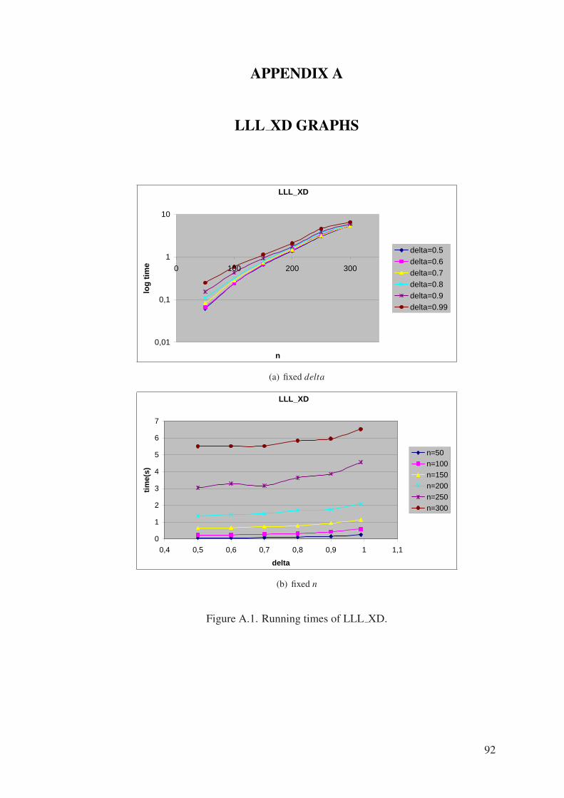
APPENDIX A
LLL XD GRAPHS
LLL_XD
0,01
0,1
1
10
0 100 200 300
n
log
tim
e
delta=0.5delta=0.6delta=0.7delta=0.8delta=0.9delta=0.99
(a) fixed delta
LLL_XD
0
1
2
3
4
5
6
7
0,4 0,5 0,6 0,7 0,8 0,9 1 1,1
delta
tim
e(s)
n=50
n=100
n=150
n=200
n=250
n=300
(b) fixed n
Figure A.1. Running times of LLL XD.
92
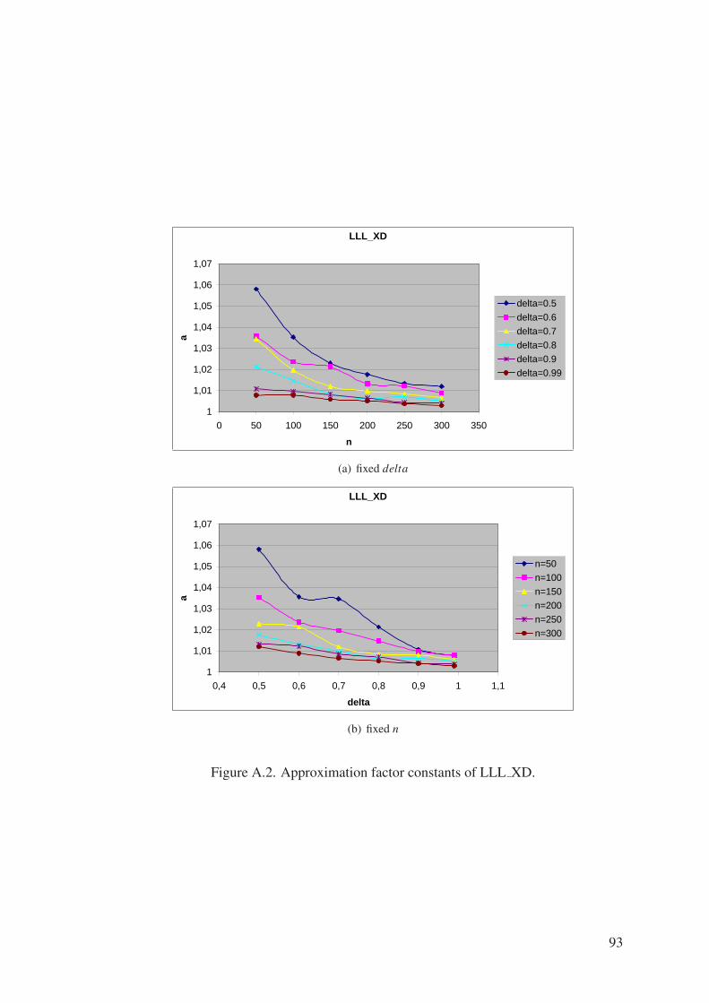
LLL_XD
1
1,01
1,02
1,03
1,04
1,05
1,06
1,07
0 50 100 150 200 250 300 350
n
a
delta=0.5
delta=0.6
delta=0.7
delta=0.8
delta=0.9
delta=0.99
(a) fixed delta
LLL_XD
1
1,01
1,02
1,03
1,04
1,05
1,06
1,07
0,4 0,5 0,6 0,7 0,8 0,9 1 1,1
delta
a
n=50
n=100
n=150
n=200
n=250
n=300
(b) fixed n
Figure A.2. Approximation factor constants of LLL XD.
93
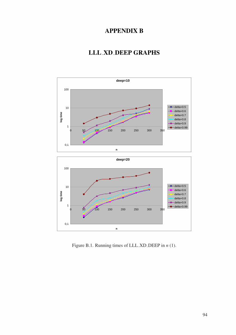
APPENDIX B
LLL XD DEEP GRAPHS
deep=10
0,1
1
10
100
0 50 100 150 200 250 300 350
n
log
tim
e
delta=0.5
delta=0.6
delta=0.7
delta=0.8
delta=0.9
delta=0.99
deep=20
0,1
1
10
100
0 50 100 150 200 250 300 350
n
log
tim
e
delta=0.5
delta=0.6
delta=0.7
delta=0.8
delta=0.9
delta=0.99
Figure B.1. Running times of LLL XD DEEP in n (1).
94

deep=30
0,1
1
10
100
1000
0 50 100 150 200 250 300 350
n
log
tim
e
delta=0.5
delta=0.6
delta=0.7
delta=0.8
delta=0.9
delta=0.99
deep=40
0,1
1
10
100
1000
10000
0 50 100 150 200 250 300 350
n
log
tim
e
delta=0.5
delta=0.6
delta=0.7
delta=0.8
delta=0.9
delta=0.99
deep=50
0,1
1
10
100
1000
10000
0 50 100 150 200 250 300 350
n
log
tim
e
delta=0.5
delta=0.6
delta=0.7
delta=0.8
delta=0.9
delta=0.99
Figure B.2. Running times of LLL XD DEEP in n (2).
95

n=50
0,1
1
10
0 10 20 30 40 50 60
deep
log
tim
e
delta=0.5
delta=0.6
delta=0.7
delta=0.8
delta=0.9
delta=0.99
n=100
0,1
1
10
100
1000
0 10 20 30 40 50 60
deep
log
tim
e
delta=0.5delta=0.6delta=0.7delta=0.8delta=0.9delta=0.99
n=150
0,1
1
10
100
1000
0 10 20 30 40 50 60
deep
log
tim
e
delta=0.5delta=0.6delta=0.7delta=0.8delta=0.9delta=0.99
Figure B.3. Running times of LLL XD DEEP in deep (1).
96

n=200
1
10
100
1000
0 10 20 30 40 50 60
deep
log
tim
e
delta=0.5delta=0.6delta=0.7delta=0.8delta=0.9delta=0.99
n=250
1
10
100
1000
0 10 20 30 40 50 60
deep
log
tim
e
delta=0.5delta=0.6delta=0.7delta=0.8delta=0.9delta=0.99
n=300
1
10
100
1000
10000
0 10 20 30 40 50 60
deep
log
tim
e
delta=0.5delta=0.6delta=0.7delta=0.8delta=0.9delta=0.99
Figure B.4. Running times of LLL XD DEEP in deep (2).
97

deep=10
0
2
4
6
8
10
12
14
16
0,4 0,5 0,6 0,7 0,8 0,9 1 1,1
delta
tim
e(s)
n=50n=100n=150n=200n=250n=300
deep=20
0
10
20
30
40
50
60
70
0,4 0,5 0,6 0,7 0,8 0,9 1 1,1
delta
tim
e(s)
n=50n=100n=150n=200n=250n=300
Figure B.5. Running times of LLL XD DEEP in delta (1).
98

deep=30
-20
0
20
40
60
80
100
120
140
160
180
200
0,4 0,5 0,6 0,7 0,8 0,9 1 1,1
delta
tim
e(s)
n=50n=100n=150n=200n=250n=300
deep=40
-200
0
200
400
600
800
1000
1200
1400
0,4 0,5 0,6 0,7 0,8 0,9 1 1,1
delta
tim
e(s)
n=50n=100n=150n=200n=250n=300
deep=50
-200
0
200
400
600
800
1000
1200
1400
1600
1800
0,4 0,5 0,6 0,7 0,8 0,9 1 1,1
delta
tim
e(s)
n=50n=100n=150n=200n=250n=300
Figure B.6. Running times of LLL XD DEEP in delta (2).
99

deep=10
1
1,002
1,004
1,006
1,008
1,01
1,012
1,014
1,016
1,018
0 50 100 150 200 250 300 350
n
a
delta=0.5
delta=0.6
delta=0.7
delta=0.8
delta=0.9
delta=0.99
deep=20
1
1,001
1,002
1,003
1,004
1,005
1,006
1,007
1,008
0 50 100 150 200 250 300 350
n
a
delta=0.5
delta=0.6
delta=0.7
delta=0.8
delta=0.9
delta=0.99
Figure B.7. Approximation factor constants of LLL XD DEEP in n (1).
100

deep=30
1
1,001
1,002
1,003
1,004
1,005
1,006
1,007
1,008
0 50 100 150 200 250 300 350
n
a
delta=0.5
delta=0.6
delta=0.7
delta=0.8
delta=0.9
delta=0.99
deep=40
1
1,001
1,002
1,003
1,004
1,005
1,006
1,007
1,008
0 50 100 150 200 250 300 350
n
a
delta=0.5
delta=0.6
delta=0.7
delta=0.8
delta=0.9
delta=0.99
deep=50
1
1,001
1,002
1,003
1,004
1,005
1,006
1,007
1,008
0 50 100 150 200 250 300 350
n
a
delta=0.5
delta=0.6
delta=0.7
delta=0.8
delta=0.9
delta=0.99
Figure B.8. Approximation factor constants of LLL XD DEEP in n (2).
101
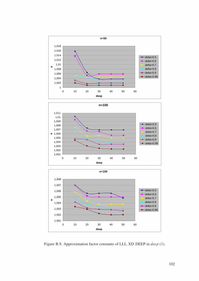
n=50
1
1,002
1,004
1,006
1,008
1,01
1,012
1,014
1,016
1,018
0 10 20 30 40 50 60
deep
a
delta=0.5
delta=0.6
delta=0.7
delta=0.8
delta=0.9
delta=0.99
n=100
1,001
1,002
1,003
1,004
1,005
1,006
1,007
1,008
1,009
1,01
1,011
0 10 20 30 40 50 60
deep
a
delta=0.5delta=0.6delta=0.7delta=0.8delta=0.9delta=0.99
n=150
1,001
1,002
1,003
1,004
1,005
1,006
1,007
1,008
0 10 20 30 40 50 60
deep
a
delta=0.5
delta=0.6
delta=0.7
delta=0.8
delta=0.9
delta=0.99
Figure B.9. Approximation factor constants of LLL XD DEEP in deep (1).
102

n=200
1,0011,00151,002
1,00251,003
1,00351,004
1,00451,005
1,00551,006
1,0065
0 10 20 30 40 50 60
deep
a
delta=0.5
delta=0.6
delta=0.7
delta=0.8
delta=0.9
delta=0.99
n=250
1,0005
1,001
1,0015
1,002
1,0025
1,003
1,0035
1,004
1,0045
0 10 20 30 40 50 60
deep
a
delta=0.5
delta=0.6
delta=0.7
delta=0.8
delta=0.9
delta=0.99
n=300
1,0005
1,001
1,0015
1,002
1,0025
1,003
1,0035
1,004
0 10 20 30 40 50 60
deep
a
delta=0.5
delta=0.6
delta=0.7
delta=0.8
delta=0.9
delta=0.99
Figure B.10. Approximation factor constants of LLL XD DEEP in deep (2).
103
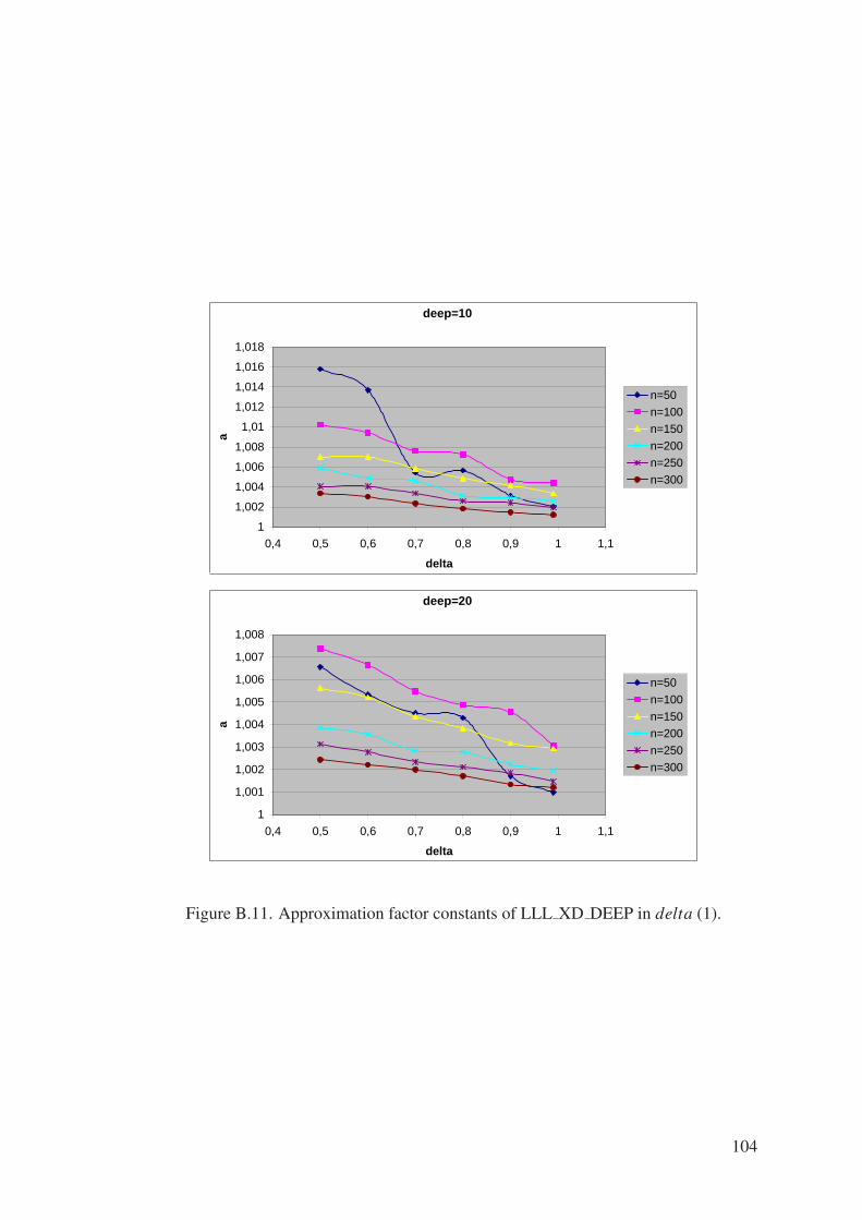
deep=10
1
1,002
1,004
1,006
1,008
1,01
1,012
1,014
1,016
1,018
0,4 0,5 0,6 0,7 0,8 0,9 1 1,1
delta
a
n=50
n=100
n=150
n=200
n=250
n=300
deep=20
1
1,001
1,002
1,003
1,004
1,005
1,006
1,007
1,008
0,4 0,5 0,6 0,7 0,8 0,9 1 1,1
delta
a
n=50
n=100
n=150
n=200
n=250
n=300
Figure B.11. Approximation factor constants of LLL XD DEEP in delta (1).
104

deep=30
1
1,001
1,002
1,003
1,004
1,005
1,006
1,007
1,008
0,4 0,5 0,6 0,7 0,8 0,9 1 1,1
delta
a
n=50
n=100
n=150
n=200
n=250
n=300
deep=40
1
1,001
1,002
1,003
1,004
1,005
1,006
1,007
1,008
0,4 0,5 0,6 0,7 0,8 0,9 1 1,1
delta
a
n=50
n=100
n=150
n=200
n=250
n=300
deep=50
1
1,001
1,002
1,003
1,004
1,005
1,006
1,007
1,008
0,4 0,5 0,6 0,7 0,8 0,9 1 1,1
delta
a
n=50
n=100
n=150
n=200
n=250
n=300
Figure B.12. Approximation factor constants of LLL XD DEEP in delta (2).
105

APPENDIX C
BKZ XD GRAPHS
blocksize=10
0,1
1
10
40 50 60 70 80 90 100 110
n
log
tim
e
delta=0.51
delta=0.6
delta=0.7
delta=0.8
delta=0.9
delta=0.99
blocksize=15
0,1
1
10
40 50 60 70 80 90 100 110
n
log
tim
e
delta=0.51
delta=0.6
delta=0.7
delta=0.8
delta=0.9
delta=0.99
Figure C.1. Running times of BKZ XD in n (1).
106
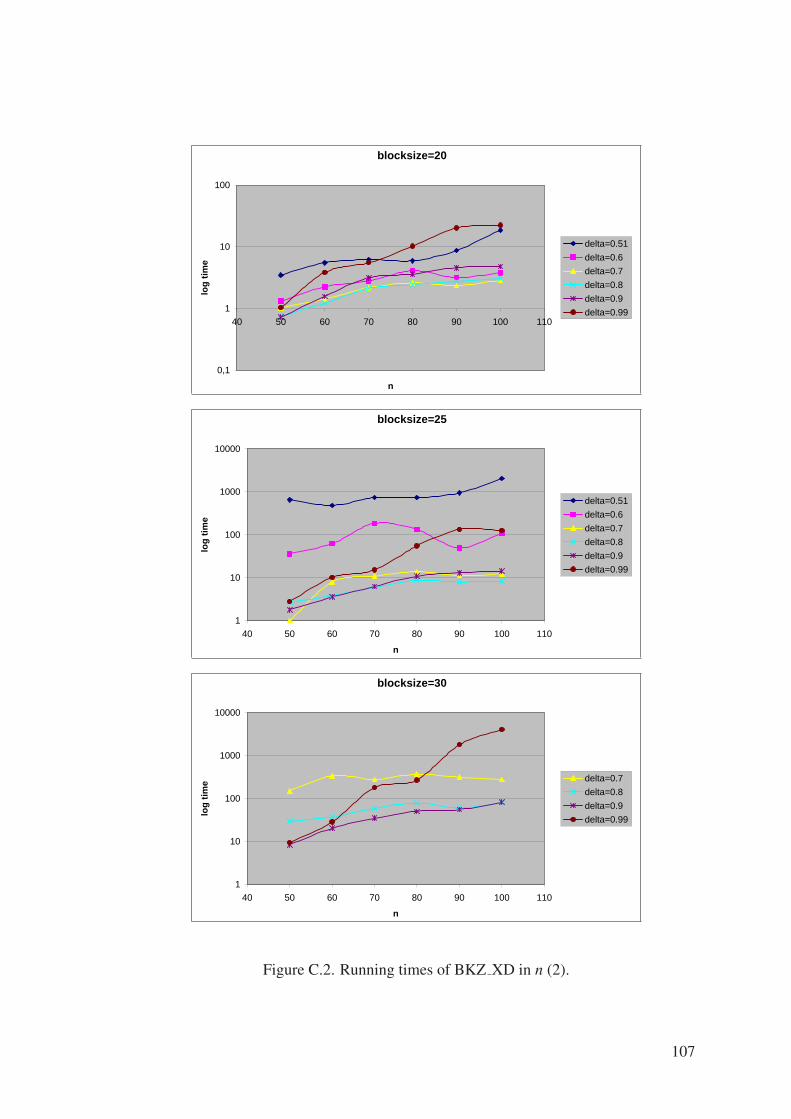
blocksize=20
0,1
1
10
100
40 50 60 70 80 90 100 110
n
log
tim
e
delta=0.51
delta=0.6
delta=0.7
delta=0.8
delta=0.9
delta=0.99
blocksize=25
1
10
100
1000
10000
40 50 60 70 80 90 100 110
n
log
tim
e
delta=0.51
delta=0.6
delta=0.7
delta=0.8
delta=0.9
delta=0.99
blocksize=30
1
10
100
1000
10000
40 50 60 70 80 90 100 110
n
log
tim
e delta=0.7
delta=0.8
delta=0.9
delta=0.99
Figure C.2. Running times of BKZ XD in n (2).
107

n=50
0,1
1
10
100
1000
0 5 10 15 20 25 30 35
blocksize
log
tim
e
delta=0.51delta=0.6delta=0.7delta=0.8delta=0.9delta=0.99
n=60
0,1
1
10
100
1000
0 5 10 15 20 25 30 35
blocksize
log
tim
e
delta=0.51delta=0.6delta=0.7delta=0.8delta=0.9delta=0.99
n=70
0,1
1
10
100
1000
0 5 10 15 20 25 30 35
blocksize
log
tim
e
delta=0.51delta=0.6delta=0.7delta=0.8delta=0.9delta=0.99
Figure C.3. Running times of BKZ XD in blocksize (1).
108

n=80
0,1
1
10
100
1000
0 5 10 15 20 25 30 35
blocksize
log
tim
e
delta=0.51delta=0.6delta=0.7delta=0.8delta=0.9delta=0.99
n=90
0,1
1
10
100
1000
10000
0 5 10 15 20 25 30 35
blocksize
log
tim
e
delta=0.51delta=0.6delta=0.7delta=0.8delta=0.9delta=0.99
n=100
0,1
1
10
100
1000
10000
0 5 10 15 20 25 30 35
blocksize
log
tim
e
delta=0.51delta=0.6delta=0.7delta=0.8delta=0.9delta=0.99
Figure C.4. Running times of BKZ XD in blocksize (2).
109
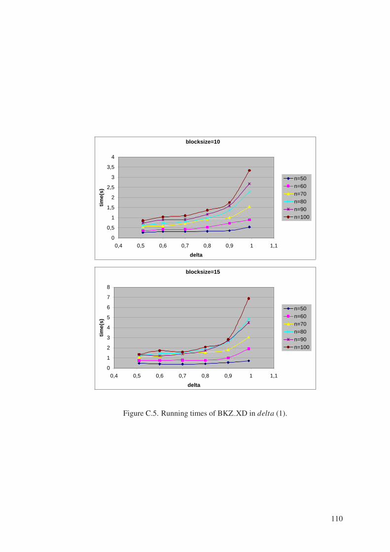
blocksize=10
0
0,5
1
1,5
2
2,5
3
3,5
4
0,4 0,5 0,6 0,7 0,8 0,9 1 1,1
delta
tim
e(s)
n=50n=60n=70n=80n=90n=100
blocksize=15
0
1
2
3
4
5
6
7
8
0,4 0,5 0,6 0,7 0,8 0,9 1 1,1
delta
tim
e(s)
n=50n=60n=70n=80n=90n=100
Figure C.5. Running times of BKZ XD in delta (1).
110

blocksize=20
0
5
10
15
20
25
0,4 0,5 0,6 0,7 0,8 0,9 1 1,1
delta
tim
e(s)
n=50n=60n=70n=80n=90n=100
blocksize=25
-500
0
500
1000
1500
2000
2500
0,4 0,5 0,6 0,7 0,8 0,9 1 1,1
delta
tim
e(s)
n=50n=60n=70n=80n=90n=100
blocksize=30
-500
0
500
1000
1500
2000
2500
3000
3500
4000
4500
0,4 0,5 0,6 0,7 0,8 0,9 1 1,1
delta
tim
e(s)
n=50n=60n=70n=80n=90n=100
Figure C.6. Running times of BKZ XD in delta (2).
111

blocksize=10
1
1,002
1,004
1,006
1,008
1,01
1,012
1,014
40 50 60 70 80 90 100 110
n
a
delta=0.51
delta=0.6
delta=0.7
delta=0.8
delta=0.9
delta=0.99
blocksize=15
1,001
1,002
1,003
1,004
1,005
1,006
1,007
1,008
1,009
1,01
40 50 60 70 80 90 100 110
n
a
delta=0.51
delta=0.6
delta=0.7
delta=0.8
delta=0.9
delta=0.99
Figure C.7. Approximation factor constants of BKZ XD in n (1).
112
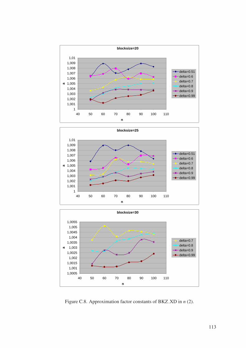
blocksize=20
1
1,001
1,002
1,003
1,004
1,005
1,006
1,007
1,008
1,009
1,01
40 50 60 70 80 90 100 110
n
a
delta=0.51
delta=0.6
delta=0.7
delta=0.8
delta=0.9
delta=0.99
blocksize=25
1
1,001
1,002
1,003
1,004
1,005
1,006
1,007
1,008
1,009
1,01
40 50 60 70 80 90 100 110
n
a
delta=0.51
delta=0.6
delta=0.7
delta=0.8
delta=0.9
delta=0.99
blocksize=30
1,0005
1,001
1,0015
1,002
1,0025
1,003
1,0035
1,004
1,0045
1,005
1,0055
40 50 60 70 80 90 100 110
n
a
delta=0.7
delta=0.8
delta=0.9
delta=0.99
Figure C.8. Approximation factor constants of BKZ XD in n (2).
113

n=50
1
1,002
1,004
1,006
1,008
1,01
1,012
0 5 10 15 20 25 30 35
blocksize
a
delta=0.51
delta=0.6
delta=0.7
delta=0.8
delta=0.9
delta=0.99
n=60
1
1,002
1,004
1,006
1,008
1,01
1,012
1,014
0 5 10 15 20 25 30 35
blocksize
a
delta=0.51delta=0.6delta=0.7delta=0.8delta=0.9delta=0.99
n=70
1
1,002
1,004
1,006
1,008
1,01
1,012
0 5 10 15 20 25 30 35
blocksize
a
delta=0.51
delta=0.6
delta=0.7
delta=0.8
delta=0.9
delta=0.99
Figure C.9. Approximation factor constants of BKZ XD in blocksize (1).
114
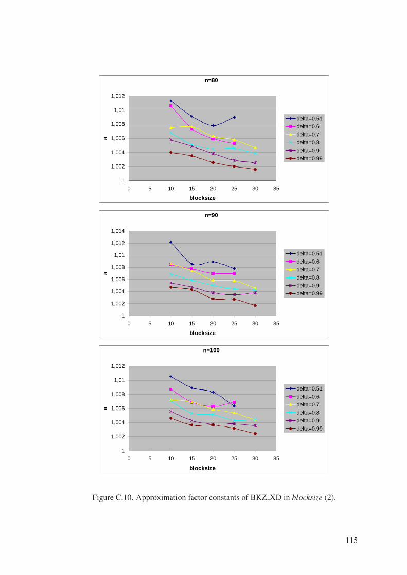
n=80
1
1,002
1,004
1,006
1,008
1,01
1,012
0 5 10 15 20 25 30 35
blocksize
a
delta=0.51
delta=0.6
delta=0.7
delta=0.8
delta=0.9
delta=0.99
n=90
1
1,002
1,004
1,006
1,008
1,01
1,012
1,014
0 5 10 15 20 25 30 35
blocksize
a
delta=0.51
delta=0.6
delta=0.7
delta=0.8
delta=0.9
delta=0.99
n=100
1
1,002
1,004
1,006
1,008
1,01
1,012
0 5 10 15 20 25 30 35
blocksize
a
delta=0.51
delta=0.6
delta=0.7
delta=0.8
delta=0.9
delta=0.99
Figure C.10. Approximation factor constants of BKZ XD in blocksize (2).
115

blocksize=10
1
1,002
1,004
1,006
1,008
1,01
1,012
1,014
0,4 0,5 0,6 0,7 0,8 0,9 1 1,1
delta
a
n=50
n=60
n=70
n=80
n=90
n=100
blocksize=15
1,001
1,002
1,003
1,004
1,005
1,006
1,007
1,008
1,009
1,01
0,4 0,5 0,6 0,7 0,8 0,9 1 1,1
delta
a
n=50
n=60
n=70
n=80
n=90
n=100
Figure C.11. Approximation factor constants of BKZ XD in delta (1).
116
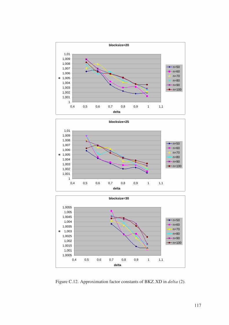
blocksize=20
1
1,001
1,002
1,003
1,004
1,005
1,006
1,007
1,008
1,009
1,01
0,4 0,5 0,6 0,7 0,8 0,9 1 1,1
delta
a
n=50
n=60
n=70
n=80
n=90
n=100
blocksize=25
1
1,001
1,002
1,003
1,004
1,005
1,006
1,007
1,008
1,009
1,01
0,4 0,5 0,6 0,7 0,8 0,9 1 1,1
delta
a
n=50
n=60
n=70
n=80
n=90
n=100
blocksize=30
1,0005
1,001
1,0015
1,002
1,0025
1,003
1,0035
1,004
1,0045
1,005
1,0055
0,4 0,5 0,6 0,7 0,8 0,9 1 1,1
delta
a
n=50
n=60
n=70
n=80
n=90
n=100
Figure C.12. Approximation factor constants of BKZ XD in delta (2).
117

APPENDIX D
COMPARISON GRAPHS
n=100
-500
0
500
1000
1500
2000
2500
3000
3500
4000
4500
0,4 0,6 0,8 1
delta
tim
e
LLL_XDLLL_XD_DEEP(10)LLL_XD_DEEP(30)LLL_XD_DEEP(50)BKZ_XD(10)BKZ_XD(20)BKZ_XD(30)
(a) fixed n = 100
n=100
-1
4
9
14
19
0,4 0,6 0,8 1
delta
tim
e
LLL_XDLLL_XD_DEEP(10)LLL_XD_DEEP(30)LLL_XD_DEEP(50)BKZ_XD(10)BKZ_XD(20)BKZ_XD(30)
(b) a closer look
Figure D.1. Comparison of running times.
118
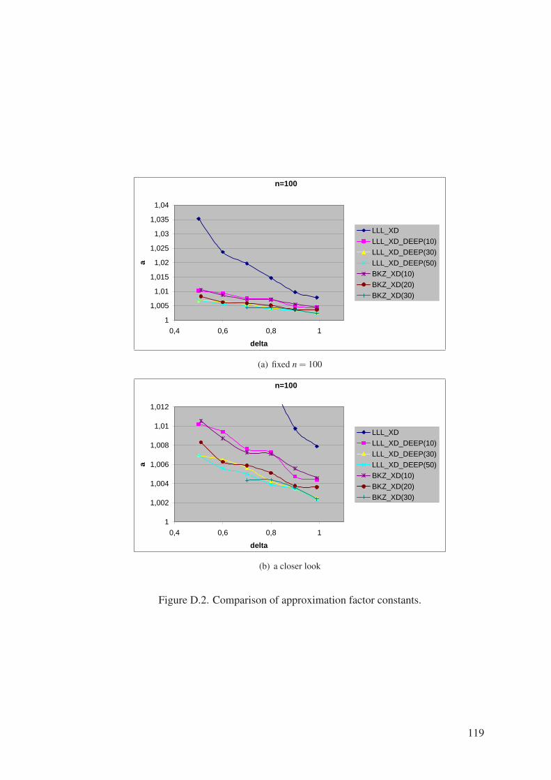
n=100
1
1,005
1,01
1,015
1,02
1,025
1,03
1,035
1,04
0,4 0,6 0,8 1
delta
a
LLL_XD
LLL_XD_DEEP(10)
LLL_XD_DEEP(30)
LLL_XD_DEEP(50)
BKZ_XD(10)
BKZ_XD(20)
BKZ_XD(30)
(a) fixed n = 100
n=100
1
1,002
1,004
1,006
1,008
1,01
1,012
0,4 0,6 0,8 1
delta
a
LLL_XD
LLL_XD_DEEP(10)
LLL_XD_DEEP(30)
LLL_XD_DEEP(50)
BKZ_XD(10)
BKZ_XD(20)
BKZ_XD(30)
(b) a closer look
Figure D.2. Comparison of approximation factor constants.
119