LUND UNIVERSITY

PO Box 117221 00 Lund+46 46-222 00 00

Reduction of vertical field taper at a ground-bounce RCS range

Larsson, Christer; Svensson, Carl-Gustaf

Published in:AMTA Proceedings

2003

Link to publication

Citation for published version (APA):Larsson, C., & Svensson, C-G. (2003). Reduction of vertical field taper at a ground-bounce RCS range. In AMTAProceedings (Vol. 25, pp. 494-499). Antenna Measurement Techniques Association.

General rightsCopyright and moral rights for the publications made accessible in the public portal are retained by the authorsand/or other copyright owners and it is a condition of accessing publications that users recognise and abide by thelegal requirements associated with these rights.

• Users may download and print one copy of any publication from the public portal for the purpose of private studyor research. • You may not further distribute the material or use it for any profit-making activity or commercial gain • You may freely distribute the URL identifying the publication in the public portalTake down policyIf you believe that this document breaches copyright please contact us providing details, and we will removeaccess to the work immediately and investigate your claim.

REDUCTION OF VERTICAL FIELD TAPER AT A GROUND-BOUNCE RCS RANGE

Christer Larsson

AerotechTelub AB, SE-581 88 Linköping, Sweden

Carl-Gustaf Svensson Saab Bofors Dynamics AB, SE-581 88 Linköping, Sweden

ABSTRACT We have investigated a method that reduces the vertical field taper at a ground-bounce radar cross-section range using a vertical antenna array. An experiment was designed were the coherent data from two measurement channels were independently recorded and stored for post processing. The two datasets were weighted and added in the post-processing to form the extended zone with improved vertical field taper. Vertically distributed point scatterers on a special test object were used to aid in optimizing the method using imaging techniques. The method is evaluated using simulations and measurements. The usefulness of this method for RCS measurements of full-scale objects such as vehicles and aircraft is discussed. We find that the method can be used to reduce the vertical field taper over a wide frequency band in the way that theory predicts. Keywords: Antenna array; Ground-bounce; ISAR; Radar imaging; RCS Measurements; Taper reduction

1. Introduction Ground-bounce radar cross section (RCS) ranges have the advantage that the power budget is improved up to 16 times compared to a range with direct illumination. One important drawback is the vertical field taper. The taper effectively reduces the useful vertical extent of the measurement volume. The common way of reducing the taper is to increase the measurement height, which often causes practical problems and high costs. Reduced vertical field taper is also often preferred for measurements on ground vehicles positioned directly on the turntable. Fisher [1] and recently Berrie [2] have previously investigated the concept of using a vertical array to change the field profile at the target. Such an array can be used to minimize the influence of the support structure and at the same time form a low taper profile for measurements of e.g. aircraft[1,2]. As pointed out in ref. 2 this array can be formed synthetically. The necessary element weights can then be applied in post

processing. The aim of the work described in this paper is to investigate the feasibility of beam forming the field using a vertical array. We do this by designing and performing an experiment with a very small array, two antennas at different heights on a ground-bounce range. The array consist of two real antennas and not of one moving antenna but we use the term synthetic array through the paper to focus on the fact that the beam forming is done in the post processing stage. We also design a special test target to aid in finding the antenna element weights and evaluate the effectiveness of the method.

2. Method A ground-bounce RCS range has a field at the measured target that consists of the coherent sum of the direct field from the transmitting antenna and the reflected field. Assuming a flat ground plane one can calculate the variation in the field at the target [3]. Simple geometrical considerations give the expressions in 1 and 2, where RD is the path length for the direct field component, RR is the path length for the reflected field, R is the horizontal range, hA is the height of the antenna and hT is the height at the target.

[ ] 2/122 )( TAD hhRR −+= (1)

[ ] 2/122 )( TAR hhRR ++= (2) A complex factor that represents the ratio between the total field and the direct field at the target is defined in 3. Here j=(-1)1/2, λ is the wavelength and ρ is the reflection coefficient of the ground.

�����

� −−+=λ

πρ )(2exp1 DR RRj

F (3)

The same multipath effects are present on the return from the target to the radar. This gives the expression in 4 for the power returned to the radar, PR [3].

44 )(2

exp1 �����

� −−+=∝λ

πρ DRR

RRjFP (4)

The reflection coefficient ρ is approximately -1 for small grazing angles. The factor |F|4 is plotted as a function of target height in figure 1 for ρ = -1 with the antenna at

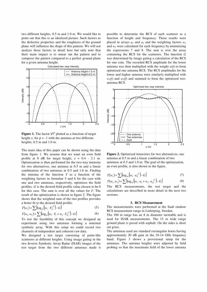
two different heights, 0.5 m and 1.0 m. We would like to point out that this is an idealized picture. Such factors as the dielectric properties and the roughness of the ground plane will influence the shape of this pattern. We will not analyze these factors in detail here but only note that their main impact is to smear out the pattern and to compress the pattern compared to a perfect ground plane for a given antenna height.

0 0.5 1 1.5 2 2.5−10

−5

0

5

10

15

20

z (m)

Inte

nsity

(dB

)

Calculated two−way intensity

Antenna height=1.0 mAntenna height=0.5 m

Figure 1. The factor |F|4 plotted as a function of target height z, for ρ = -1 with the antenna at two different heights, 0.5 m and 1.0 m. The main idea of this paper can be shown using the data from figure 1. We assume that we want an even field profile at 0 dB for target height, z = 0.4 - 2.1 m. Optimization is then performed for the two-way intensity for two alternatives, one antenna at 0.5 m and a linear combination of two antennas at 0.5 and 1.0 m. Finding the minima of the function T as a function of the weighting factors in formulae 5 and 6 for the case with one and two antennas, respectively, optimizes the field profiles. G is the desired field profile value chosen to be 0 for this case. The sum is over all the values for F. The result of the optimization is shown in figure 2. The figure shows that the weighted sum of the two profiles provides a better fit to the desired field profile.

( ) ( )( )� −⋅= GFwwT4

11101 log (5)

( ) ( )( )� −⋅+⋅= GFwFwwwT4

22111021 log, (6)

To test the feasibility of this concept we designed an experiment using two antennas forming a minimal synthetic array. With this setup we could record two channels of independent and coherent raw data. We designed a test target consisting of point-like scatterers at different heights. Using image gating in the two Inverse Synthetic Array Radar (ISAR) images of the test target from the two different antennas made it

possible to determine the RCS of each scatterer as a function of height and frequency. These results were placed in arrays a1 and a2 and the weighting factors w1 and w2 were calculated for each frequency by minimizing the expressions 7 and 8. The sum is over the array containing the RCS for the scatterers. The function G was determined by image gating a calculation of the RCS for one coin. The recorded RCS amplitude for the lower antenna was then multiplied with the weight w(f) to form optimized one antenna RCS. The RCS amplitudes for the lower and higher antenna were similarly multiplied with w1(f) and w2(f) and summed to form the optimized two-antenna RCS.

0 0.5 1 1.5 2 2.5−25

−20

−15

−10

−5

0

5

z (m)

Inte

nsity

(dB

)

Optimized two−way intensity

One antennaTwo antennasGoal

Figure 2. Optimized intensities for two alternatives, one antenna at 0.5 m and a linear combination of two antennas at 0.5 and 1.0 m. The goal of the optimization, an even profile, is also shown in the figure.

( ) ( )( )� −⋅= GawwT2

11101 log (7)

( ) ( )( )� −⋅+⋅= GawawwwT2

22111021 log, (8)

The RCS measurements, the test target and the calculations are described in more detail in the next two sections.

3. RCS Measurement The measurements were performed at the Saab outdoor RCS measurement range in Linköping, Sweden. The 100 m range has an 8 m diameter turntable and is used for ISAR measurements. The 15 m wide range ground plane is paved with asphalt. On the sides is short cut grass. The antennas used are standard rectangular horns having approximately 20 dB gain in the 10-14 GHz frequency band. Figure 3 shows a provisional setup for the antennas. The antenna heights were adjusted by field probing so that the maximum field of the lower antenna

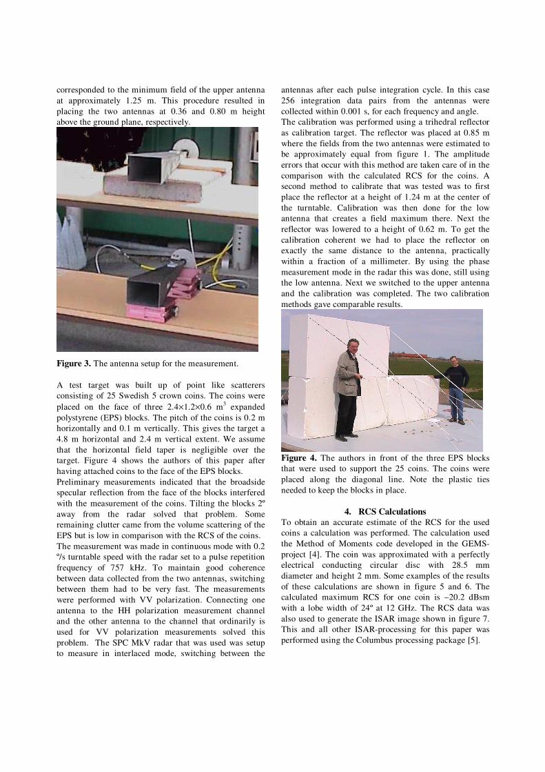
corresponded to the minimum field of the upper antenna at approximately 1.25 m. This procedure resulted in placing the two antennas at 0.36 and 0.80 m height above the ground plane, respectively.

Figure 3. The antenna setup for the measurement. A test target was built up of point like scatterers consisting of 25 Swedish 5 crown coins. The coins were placed on the face of three 2.4×1.2×0.6 m3 expanded polystyrene (EPS) blocks. The pitch of the coins is 0.2 m horizontally and 0.1 m vertically. This gives the target a 4.8 m horizontal and 2.4 m vertical extent. We assume that the horizontal field taper is negligible over the target. Figure 4 shows the authors of this paper after having attached coins to the face of the EPS blocks. Preliminary measurements indicated that the broadside specular reflection from the face of the blocks interfered with the measurement of the coins. Tilting the blocks 2º away from the radar solved that problem. Some remaining clutter came from the volume scattering of the EPS but is low in comparison with the RCS of the coins. The measurement was made in continuous mode with 0.2 º/s turntable speed with the radar set to a pulse repetition frequency of 757 kHz. To maintain good coherence between data collected from the two antennas, switching between them had to be very fast. The measurements were performed with VV polarization. Connecting one antenna to the HH polarization measurement channel and the other antenna to the channel that ordinarily is used for VV polarization measurements solved this problem. The SPC MkV radar that was used was setup to measure in interlaced mode, switching between the

antennas after each pulse integration cycle. In this case 256 integration data pairs from the antennas were collected within 0.001 s, for each frequency and angle. The calibration was performed using a trihedral reflector as calibration target. The reflector was placed at 0.85 m where the fields from the two antennas were estimated to be approximately equal from figure 1. The amplitude errors that occur with this method are taken care of in the comparison with the calculated RCS for the coins. A second method to calibrate that was tested was to first place the reflector at a height of 1.24 m at the center of the turntable. Calibration was then done for the low antenna that creates a field maximum there. Next the reflector was lowered to a height of 0.62 m. To get the calibration coherent we had to place the reflector on exactly the same distance to the antenna, practically within a fraction of a millimeter. By using the phase measurement mode in the radar this was done, still using the low antenna. Next we switched to the upper antenna and the calibration was completed. The two calibration methods gave comparable results.

Figure 4. The authors in front of the three EPS blocks that were used to support the 25 coins. The coins were placed along the diagonal line. Note the plastic ties needed to keep the blocks in place.

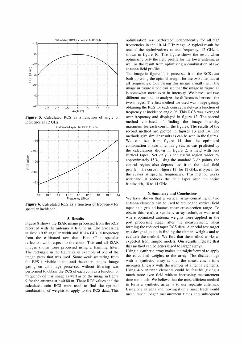
4. RCS Calculations To obtain an accurate estimate of the RCS for the used coins a calculation was performed. The calculation used the Method of Moments code developed in the GEMS-project [4]. The coin was approximated with a perfectly electrical conducting circular disc with 28.5 mm diameter and height 2 mm. Some examples of the results of these calculations are shown in figure 5 and 6. The calculated maximum RCS for one coin is –20.2 dBsm with a lobe width of 24º at 12 GHz. The RCS data was also used to generate the ISAR image shown in figure 7. This and all other ISAR-processing for this paper was performed using the Columbus processing package [5].

−15 −10 −5 0 5 10 15−45

−40

−35

−30

−25

−20

−15

Angle (°)

RC

S (d

Bsm

)

Calculated RCS for coin at f=12 GHz

Figure 5. Calculated RCS as a function of angle of incidence at 12 GHz.

10 10.5 11 11.5 12 12.5 13 13.5 14

−21

−20.5

−20

−19.5

−19

RC

S (d

Bsm

)

Frequency (GHz)

Calculated specular RCS for coin

Figure 6. Calculated RCS as a function of frequency for specular incidence.

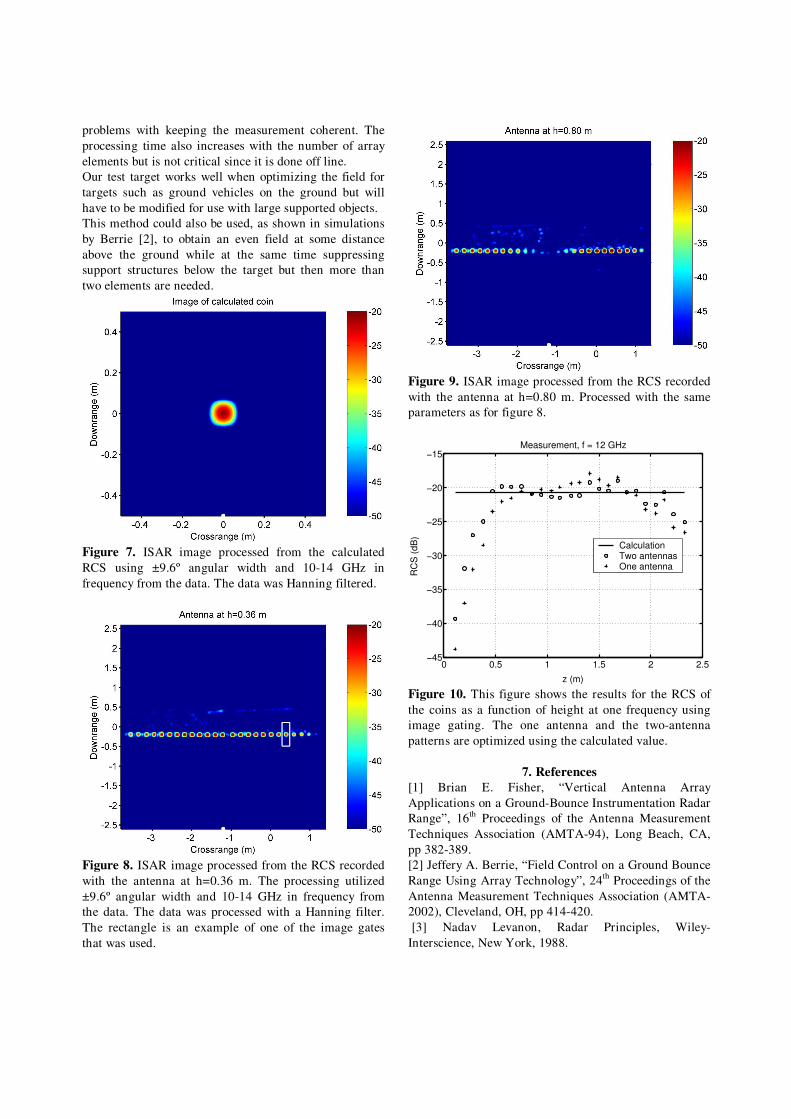
5. Results Figure 8 shows the ISAR image processed from the RCS recorded with the antenna at h=0.36 m. The processing utilized ±9.6º angular width and 10-14 GHz in frequency from the calibrated raw data. Here 0º is specular reflection with respect to the coins. This and all ISAR images shown were processed using a Hanning filter. The rectangle in the figure is an example of one of the image gates that was used. Some weak scattering from the EPS is visible in this and the other images. Image gating on an image processed without filtering was performed to obtain the RCS of each coin as a function of frequency on this image as well as on the image in figure 9 for the antenna at h=0.80 m. These RCS values and the calculated coin RCS were used to find the optimal combination of weights to apply to the RCS data. This

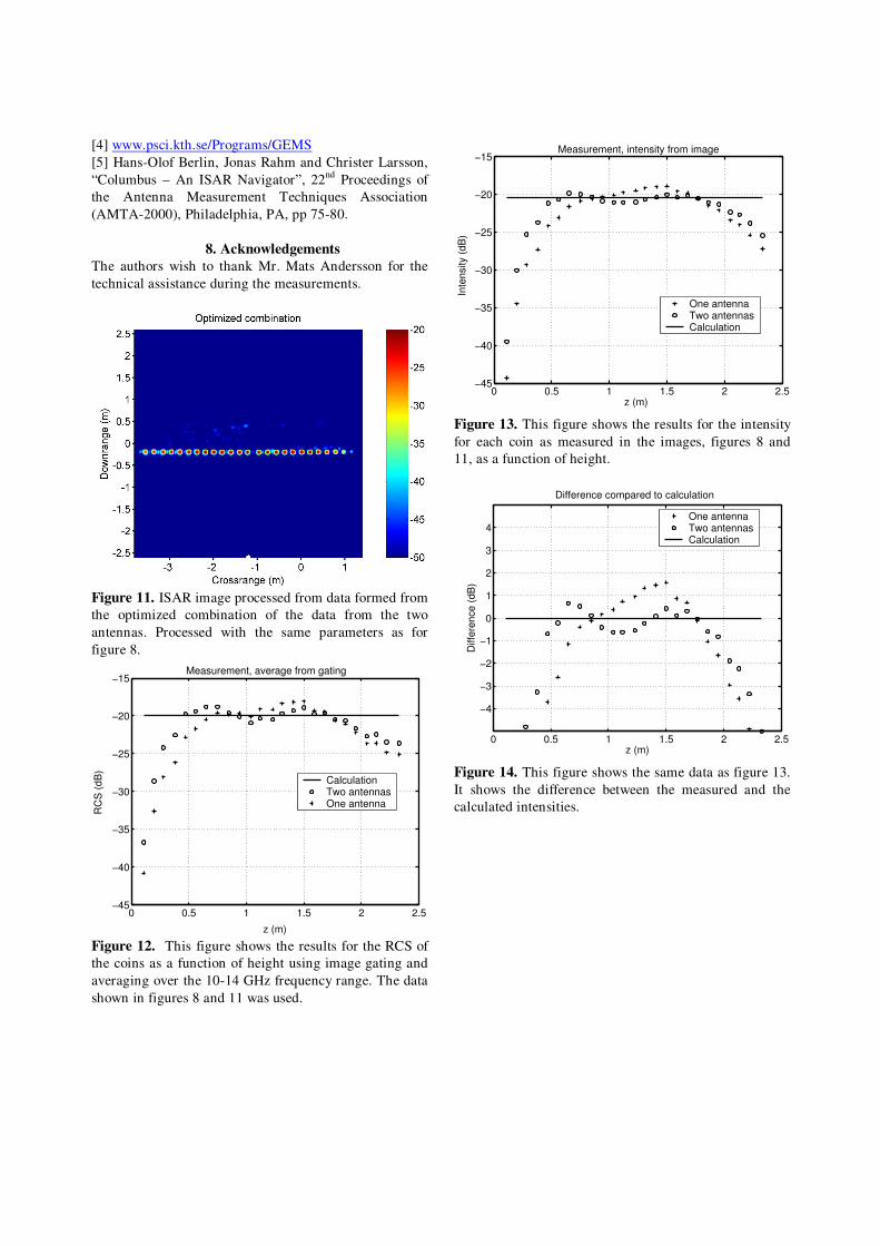
optimization was performed independently for all 512 frequencies in the 10-14 GHz range. A typical result for one of the optimizations at one frequency, 12 GHz is shown in figure 10. This figure shows the result when optimizing only the field profile for the lower antenna as well as the result from optimizing a combination of two antenna field profiles. The image in figure 11 is processed from the RCS data built up using the optimal weight for the two antennas at all frequencies. Comparing this image visually with the image in figure 8 one can see that the image in figure 11 is somewhat more even in intensity. We have used two different methods to analyze the differences between the two images. The first method we used was image gating, obtaining the RCS for each coin separately as a function of frequency at incidence angle 0º. This RCS was averaged over frequency and displayed in figure 12. The second method consisted of finding the image intensity maximum for each coin in the figures. The results of the second method are plotted in figures 13 and 14. The methods give similar results as can be seen in the figures. We can see from figure 14 that the optimized combination of two antennas gives, as was predicted by the calculations shown in figure 2, a field with less vertical taper. Not only is the useful region wider by approximately 15%, using the standard 3 db points, the central region also departs less from the ideal field profile. The curve in figure 12, for 12 GHz, is typical for the curves at specific frequencies. This method works wideband; it reduces the field taper over the entire bandwidth, 10 to 14 GHz.

6. Summary and Conclusions We have shown that a vertical array consisting of two antenna elements can be used to reduce the vertical field taper at a ground-bounce radar cross-section range. To obtain this result a synthetic array technique was used where optimized antenna weights were applied in the post processing stage, after the measurement, when forming the reduced taper RCS data. A special test target was designed to aid in finding the element weights and to evaluate the method. We find that the method works as expected from simple models. Our results indicate that this method can be generalized to larger arrays. Using a synthetic array makes it straightforward to apply the calculated weights to the array. The disadvantage with a synthetic array is that the measurement time increases linearly with the number of antenna elements. Using 4-6 antenna elements could be feasible giving a much more even field without increasing measurement time too much. We believe that the most efficient method to form a synthetic array is to use separate antennas. Using one antenna and moving it on a linear track would mean much longer measurement times and subsequent

problems with keeping the measurement coherent. The processing time also increases with the number of array elements but is not critical since it is done off line. Our test target works well when optimizing the field for targets such as ground vehicles on the ground but will have to be modified for use with large supported objects. This method could also be used, as shown in simulations by Berrie [2], to obtain an even field at some distance above the ground while at the same time suppressing support structures below the target but then more than two elements are needed.

Figure 7. ISAR image processed from the calculated RCS using ±9.6º angular width and 10-14 GHz in frequency from the data. The data was Hanning filtered.

Figure 8. ISAR image processed from the RCS recorded with the antenna at h=0.36 m. The processing utilized ±9.6º angular width and 10-14 GHz in frequency from the data. The data was processed with a Hanning filter. The rectangle is an example of one of the image gates that was used.

Figure 9. ISAR image processed from the RCS recorded with the antenna at h=0.80 m. Processed with the same parameters as for figure 8.

0 0.5 1 1.5 2 2.5−45

−40

−35

−30

−25

−20

−15Measurement, f = 12 GHz

z (m)

RC

S (d

B)

CalculationTwo antennasOne antenna

Figure 10. This figure shows the results for the RCS of the coins as a function of height at one frequency using image gating. The one antenna and the two-antenna patterns are optimized using the calculated value.

7. References [1] Brian E. Fisher, “Vertical Antenna Array Applications on a Ground-Bounce Instrumentation Radar Range”, 16th Proceedings of the Antenna Measurement Techniques Association (AMTA-94), Long Beach, CA, pp 382-389. [2] Jeffery A. Berrie, “Field Control on a Ground Bounce Range Using Array Technology”, 24th Proceedings of the Antenna Measurement Techniques Association (AMTA-2002), Cleveland, OH, pp 414-420. [3] Nadav Levanon, Radar Principles, Wiley-Interscience, New York, 1988.

[4] www.psci.kth.se/Programs/GEMS [5] Hans-Olof Berlin, Jonas Rahm and Christer Larsson, “Columbus – An ISAR Navigator”, 22nd Proceedings of the Antenna Measurement Techniques Association (AMTA-2000), Philadelphia, PA, pp 75-80.

8. Acknowledgements The authors wish to thank Mr. Mats Andersson for the technical assistance during the measurements.

Figure 11. ISAR image processed from data formed from the optimized combination of the data from the two antennas. Processed with the same parameters as for figure 8.

0 0.5 1 1.5 2 2.5−45

−40

−35

−30

−25

−20

−15

z (m)

RC

S (d

B)

Measurement, average from gating

CalculationTwo antennasOne antenna

Figure 12. This figure shows the results for the RCS of the coins as a function of height using image gating and averaging over the 10-14 GHz frequency range. The data shown in figures 8 and 11 was used.

0 0.5 1 1.5 2 2.5−45

−40

−35

−30

−25

−20

−15

z (m)

Inte

nsity

(dB

)

Measurement, intensity from image

One antennaTwo antennasCalculation

Figure 13. This figure shows the results for the intensity for each coin as measured in the images, figures 8 and 11, as a function of height.

0 0.5 1 1.5 2 2.5

−4

−3

−2

−1

0

1

2

3

4

Difference compared to calculation

z (m)

Diff

eren

ce (d

B)

One antennaTwo antennasCalculation

Figure 14. This figure shows the same data as figure 13. It shows the difference between the measured and the calculated intensities.