arX

iv:1

602.

0611

5v1

[co

nd-m

at.s

tat-

mec

h] 1

9 Fe

b 20

16

Reentrance of disorder in the anisotropic shuriken Ising model

Rico Pohle,1 Owen Benton,1 and L.D.C. Jaubert1

1Okinawa Institute of Science and Technology Graduate University, Onna-son, Okinawa 904-0495, Japan

(Dated: February 22, 2016)

For a material to order upon cooling is common sense. What is more seldom is for disorder toreappear at lower temperature, which is known as reentrant behavior. Such resurgence of disorderhas been observed in a variety of systems, ranging from Rochelle salts to nematic phases in liquidcrystals. Frustration is often a key ingredient for reentrance mechanisms. Here we shall study afrustrated model, namely the anisotropic shuriken lattice, which offers a natural setting to explore anextension of the notion of reentrance between magnetic disordered phases. By tuning the anisotropyof the lattice, we open a window in the phase diagram where magnetic disorder prevails down to zerotemperature. In this region, the competition between multiple disordered ground states gives rise toa double crossover where both the low- and high-temperature regimes are less correlated than theintervening classical spin liquid. This reentrance of disorder is characterized by an entropy plateau,a multi-step Curie law crossover and a rather complex diffuse scattering in the static structurefactor. Those results are confirmed by complementary numerical and analytical methods: MonteCarlo simulations, Husimi-tree calculations and an exact decoration-iteration transformation.

PACS numbers: 75.10.Hk,75.30.Kz,75.10.Kt

Recent progress in frustrated magnetism has deliv-ered entire maps of long-range ordered and disorderedphases, obtained for example via the variation of bondanisotropy1–7 or further nearest-neighbour couplings8–14.Such phase diagrams have allowed to put a series of frus-trated materials onto a global and connected map, thatcan be experimentally explored via physical or chemi-cal pressure15–18. On such phase diagrams, when twoordered phases meet, an enhancement of the classicalground-state degeneracy takes place19. This degeneracycan either be lifted by thermal fluctuations, giving rise tomultiple phase transitions20,21, or may destroy any kindof order down to (theoretically) zero temperature. This iswhere spin liquids appear. But this picture is less clear atthe frontier between ordered and (possibly multiple) dis-ordered ground states. In particular how do disorderedphases compete with each other at finite temperature ?

The frustrated shuriken lattice22 – also known assquare-kagome23–30, squagome31,32, squa-kagome33 orL4-L833 lattice – provides an interesting model-examplefor such competition. Being made of corner-sharingtriangles, it is locally similar to the famous kagome lat-tice, but with the important difference that the shurikenlattice is composed of two inequivalent sublattices [seeFig. 1]. Such asymmetry offers a natural setup for latticeanisotropy. In the asymptotic limits of this anisotropy, apromising zero-temperature phase diagram has emergedfor quantum spin−1/2, ranging from a bipartite long-range ordered phase to a highly degenerate ground statemade of tetramer clusters of spins33. However, whilethe quantum ground states22,26,30,33 and the influenceof a magnetic field22,24–29,34 have been studied to someextent, little is known about the finite-temperatureproperties in zero field23,31.

In this paper, our goal is to develop a comprehensiveand precise understanding of the frustrated phase

FIG. 1. The shuriken lattice as seen in real space (left) andFourier space (right). There are 6 sites per unit-cell with twosublattices A and B. Interactions between A-sites (squareplaquettes) are described with coupling constant JAA (red),while interactions between A- and B-sites (octagonal plaque-ttes) are described with JAB (black).

diagram of the Ising model on the anisotropic shurikenlattice, relying on a combination of numerical andanalytical methods (Monte Carlo simulations, Husimitree calculations and decoration-iteration transfor-mation). Using the lattice anisotropy as a tuningparameter, we find that this model supports two long-range ordered phases (ferromagnet (FM) and staggeredferromagnet (SFM)), two classical spin liquids (SL1,2)characterized by complex static structure factors, anda zero-temperature paramagnet composed of two kindsof isolated (super)spins with strictly zero correlationsbetween them. We shall refer to this latter phase asa binary paramagnet. Over an extended region of thephase diagram, there is a double crossover from thehigh-temperature paramagnet to the spin liquids andfinally into the low-temperature binary paramagnet.This double crossover gives rise to a non-monotonicbehavior of the correlation length, which can be seen asan analogue of reentrant behavior between disordered

2

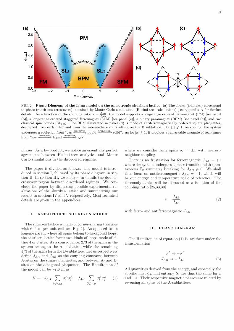
FIG. 2. Phase Diagram of the Ising model on the anisotropic shuriken lattice. (a) The circles (triangles) correspondto phase transitions (crossovers), obtained by Monte Carlo simulations (Husimi-tree calculations) [see appendix A for further

details]. As a function of the coupling ratio x = JAB

JAA, the model supports a long-range ordered ferromagnet (FM) [see panel

(b)], a long-range ordered staggered ferromagnet (SFM) [see panel (c)], a binary paramagnet (BPM) [see panel (d)], and twoclassical spin liquids (SL1,2). The BPM illustrated in panel (d) is made of antiferromagnetically ordered square plaquettes,decoupled from each other and from the intermediate spins sitting on the B sublattice. For |x| & 1, on cooling, the system

undergoes a evolution from “gascrossover−−−−−−→ liquid

transition−−−−−−→ solid”. As for |x| . 1, it provides a remarkable example of reentrance

from “gascrossover−−−−−−→ liquid

crossover−−−−−−→ gas”.

phases. As a by-product, we notice an essentially perfectagreement between Husimi-tree analytics and MonteCarlo simulations in the disordered regimes.

The paper is divided as follows. The model is intro-duced in section I, followed by its phase diagram in sec-tion II. In section III, we analyze in details the double-crossover region between disordered regimes. We con-clude the paper by discussing possible experimental re-alizations of the shuriken lattice and summarizing ourresults in sections IV and V respectively. Most technicaldetails are given in the appendices.

I. ANISOTROPIC SHURIKEN MODEL

The shuriken lattice is made of corner-sharing triangleswith 6 sites per unit cell [see Fig. 1]. As opposed to itskagome parent where all spins belong to hexagonal loops,the shuriken lattice forms two kinds of loops made of ei-ther 4 or 8 sites. As a consequence, 2/3 of the spins in thesystem belong to the A-sublattice, while the remaining1/3 of the spins form the B-sublattice. Let us respectivelydefine JAA and JAB as the coupling constants betweenA-sites on the square plaquettes, and between A- and B-sites on the octagonal plaquettes. The Hamiltonian ofthe model can be written as:

H = −JAA

∑

〈ij〉AA

σAi σ

Aj − JAB

∑

〈ij〉AB

σAi σ

Bj (1)

where we consider Ising spins σi = ±1 with nearest-neighbor coupling.

There is no frustration for ferromagnetic JAA = +1where the system undergoes a phase transition with spon-taneous Z2 symmetry breaking for JAB 6= 0. We shallthus focus on antiferromagnetic JAA = −1, which willbe our energy and temperature scale of reference. Thethermodynamics will be discussed as a function of thecoupling ratio [25,33,30]

x =JAB

JAA, (2)

with ferro- and antiferromagnetic JAB.

II. PHASE DIAGRAM

The Hamiltonian of equation (1) is invariant under thetransformation

σA → −σA

JAB → −JAB (3)

All quantities derived from the energy, and especially thespecific heat Ch and entropy S, are thus the same for xand −x. Their respective magnetic phases are related byreversing all spins of the A-sublattices.

3

A. Long-range order: |x| > 1

When the octagonal plaquettes are dominating (x →±∞), the shuriken lattice becomes a decorated squarelattice, with A-sites sitting on the bonds between B-sites. Being bipartite, the decorated square lattice isnot frustrated and orders via a phase transition of the2D Ising Universality class35 by spontaneous Z2 sym-metry breaking. Non-universal quantities such as thetransition temperature can be exactly computed by us-ing the decoration-iteration transformation35–37 [see ap-pendix D2]

Tc =2JAB

ln(√

2 + 1 +√

2 + 2√2) ≈ 1.30841JAB (4)

The low-temperature ordered phases, displayed inFig. 2.(b) and 2.(c), remain the ground states of theanisotropic shuriken model for x < −1 and x > 1 re-spectively. The persistence of the 2D Ising Universalityclass down to |x| = 1+ is not necessarily obvious, but isconfirmed by finite-size scaling from Monte Carlo simu-lations [see appendix C].These two ordered phases are respectively ferromag-

netic (FM, x < −1) and staggered ferromagnetic (SFM,x > 1) [see Fig. 2.(b,c)]. The staggering of the lattercomes from all spins on square plaquettes pointing inone direction, while the remaining ones point the otherway. This leads to the rather uncommon consequencethat fully antiferromagnetic couplings – both JAA andJAB are negative for x > 1 – induce long-range or-dered (staggered) ferromagnetism, reminiscent of Liebferrimagnetism38 as pointed out in Ref. [33] for quantumspins. The existence of ferromagnetic states among theset of ground states of Ising antiferromagnets is not rare,with the triangular and kagome lattices being two famousexamples. But such ferromagnetic states are usually partof a degenerate ensemble where no magnetic order pre-vails on average. Here the lattice anisotropy is able to in-duce ferromagnetic order in an antiferromagnetic modelby lifting its ground-state degeneracy at |x| = 1 (see be-low). This is interestingly quite the opposite of what hap-pens in the spin-ice model39, where frustration preventsmagnetic order in a ferromagnetic model by stabilizing ahighly degenerate ground state.

B. Binary paramagnet: |x| < 1

The central part of the phase diagram is dominated bythe square plaquettes. The ground states are the samefor all |x| < 1. A sample configuration of these groundstates is given in Fig. 2.(d), where antiferromagneticallyordered square-plaquettes are separated from each othervia spins on sublattice B. The antiferromagnetic square-plaquettes locally order in two different configurationsequivalent to a superspin Ξ with Ising degree of freedom.

Ξ = σA1 − σA

2 − σA3 + σA

4 = ±4, (5)

where the site indices are given in Fig. 1. These super-spins are the classical analogue of the tetramer objectsobserved in the spin−1/2 model33. At zero temperature,the frustration of the JAB bonds perfectly decouples thesuperspins Ξ from the B-sites. The system can then beseen as two interpenetrating square lattices: one madeof superspins, the other one of B-sites. We shall refer tothis phase as a binary paramagnet (BPM).The perfect absence of correlations beyond square pla-

quettes at T = 0 allows for a simple determination ofthe thermodynamics. Let Nuc and N = 6Nuc be re-spectively the total number of unit cells and spins in thesystem, and 〈X〉 be the statistical average of X . Thereare Nuc square plaquettes and 2Nuc B-sites, giving riseto an extensive ground-state entropy

SBPM = kB ln(

2Nuc 22Nuc)

=N

2kB ln 2 (6)

which turns out to be half the entropy of an Ising para-magnet. As for the magnetic susceptibility χ, it divergesas T → 0+. But the reduced susceptibility χT , which isnothing less than the normalized variance of the magne-tization

χT =1

N

∑

i,j

〈σiσj〉 − 〈σi〉〈σj〉

,

= 1 +1

N

∑

i6=j

〈σiσj〉, (7)

converges to a finite value in the BPM

χT |BPM =1

3. (8)

C. Classical spin liquid: |x| ∼ 1

There is a sharp increase of the ground-state degen-eracy at |x| = 1, when the binary paramagnet andthe (staggered) ferromagnet meet. As is common forisotropic triangle-based Ising antiferromagnets, 6 out of 8possible configurations per triangle minimize the energyof the system. As opposed to the BPM one does not ex-pect a cutoff of the correlations [see section III C], makingthese phases cooperative paramagnets40, also known asclassical spin liquids.Due to the high entropy of these cooperative paramag-

nets, the SL1,2 phases spread to the neighboring regionof the phase diagram for |x| ∼ 1 and T > 0, contin-uously connected to the high-temperature paramagnet[see Fig. 2]. Hence, for |x| & 1, the anisotropic shurikenmodel stabilizes a cooperative paramagnet above a non-degenerate41 long-range ordered phase. This is a gen-eral property of classical spin liquids when adiabaticallytuned away from their high-degeneracy point, as ob-served for example in Heisenberg antiferromagnets on thekagome42 or pyrochlore43–45 lattices, and possibly in thematerial of Er2Sn2O7

19. For |x| . 1 on the other hand,

4

FIG. 3. Multiple crossovers between the paramagnetic, spin-liquids and binary regimes as observed in the specificheat Ch, entropy S and reduced magnetic susceptibility χT . The models correspond to a) x = ±1, b) x = ±0.9 and c) x = 0.There is no phase transition for this set of parameters, which is why the Husimi tree calculations (lines) perfectly match theMonte Carlo simulations (circles) for all temperatures. The double crossover is present for x = ±0.9, with the low-temperatureregime being the same as for x = 0, as confirmed by its entropy and susceptibility. The entropy is obtained by integration ofCh/T , setting S(T → +∞) = ln 2. The vertical dashed lines represent estimates of the crossover temperatures determined bythe local specific-heat maxima. The temperature axis is on a logarithmic scale. All quantities are given per number of spinsand the Boltzmann constant kB is set to 1.

multiple crossovers take place upon cooling which de-serves a dedicated discussion in the following section III.

III. REENTRANCE OF DISORDER

A. Double crossover

First of all, panels (a) and (c) of Fig. 3 confirm thatthe classical spin liquids and binary paramagnet persistdown to zero temperature for x = ±1 and x = 0 respec-tively, and that all models for |x| 6 1 have extensivelydegenerate ground states. For x = ±0.9 there is a dou-ble crossover indicated by the double peaks in the spe-cific heat Ch of Fig. 3.(b). These peaks are not due tophase transitions since they do not diverge with systemsize. The double crossover persists for 0.5 . |x| < 1.Upon cooling, the system first evolves from the standardparamagnet to a spin liquid before entering the binary

paramagnet. The intervening spin liquid takes the formof an entropy plateau for |x| = 0.9 [see Fig. 3.(b)], atthe same value as the low-temperature regime for |x| = 1[see Fig. 3.(a)]. All relevant thermodynamic quantitiesare summarized in Table I.

While the mapping of equation (3) ensures the invari-ance of the energy, specific heat and entropy upon revers-ing x to −x, it does not protect the magnetic susceptibil-ity. The build up of correlations in classical spin liquids isknown to give rise to a Curie-law crossover46 between two1/T asymptotic regimes of the susceptibility, as observedin pyrochlore46–49, triangular50 and kagome50–52 systems.This is also what is observed here on the anisotropicshuriken lattice for x = −1, 0, 1 [see Fig. 4]. But for in-termediate models with x = −0.99,−0.9, 0.9, 0.99, thedouble crossover makes the reduced susceptibility non-monotonic. χT first evolves towards the values of thespin liquids SL1 (resp. SL2) for x < 0 (resp. x > 0)before converging to 1/3 in the binary paramagnet.

5

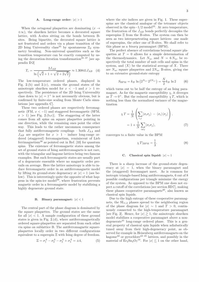
T → 0+ Monte Carlo Husimi tree exact

S(|x| = 1) 0.504(1)1

6ln

41

2≈ 0.5034 n/a

χT (x = 1) 0.203(1) 0.2028 n/a

χT (x = −1) 1.766(1) 1.771 n/a

S(|x| < 1) 0.347(1)1

2ln 2 ≈ 0.3466

1

2ln 2

χT (|x| < 1) 0.333(1)1

3

1

3

TABLE I. Entropies S and reduced susceptibilities χTas T → 0+ for the anisotropic shuriken lattice with couplingratios |x| 6 1. The results are obtained from Monte Carlosimulations, Husimi tree analytics and the exact solution forthe binary paramagnet. All quantities are given per numberof spins and the Boltzmann constant kB is set to 1.

FIG. 4. Reduced susceptibility χT with coupling ratiosof x = ±1,±0.99,±0.9 and 0, obtained from Husimi-tree cal-culations (solid lines) and Monte Carlo simulations (circles).The Curie-law crossover of classical spin liquids is standard,i.e. χT is monotonic, for x = ±1 and 0, and takes a multi-step behavior for intermediate values of x, due to the doublecrossover. The characteristic values of the entropy and re-duced susceptibility are given in Table I. The temperatureaxis is on a logarithmic scale

Beyond the present problem on the shuriken lattice,this multi-step Curie-law crossover underlines the use-fulness of the reduced susceptibility to spot intermedi-ate regimes, and thus the proximity of different phases.From the point of view of renormalization group theory,the (x, T ) = (±1, 0) coordinates of the phase diagramare fixed points which deform the renormalization flowspassing in the vicinity.

B. Decoration-iteration transformation

The phase diagram of the anisotropic shuriken modeland, in particular, the double crossover observed for|x| < 1 [see Fig. 2] can be further understood using anexact mapping to an effective model on the checkerboardlattice, a method known as decoration-iteration transfor-mation [see Ref. [37] for a review]. In short, by summingover the degrees of freedom of the A-spins, one can arriveat an effective Hamiltonian involving only the B-spins,which form a checkerboard lattice. The coupling con-stants of the effective Hamiltonian are functions of thetemperature T and for |x| < 1 they vanish at both highand low temperatures, but are finite for an intermedi-ate regime. This intermediate regime may be identifiedas the SL1,2 cooperative paramagnets of Fig. 2, whereasthe low-temperature region of vanishing effective interac-tion corresponds to the binary paramagnet (BPM). Thismapping is able to predict a non-monotonic behavior ofthe correlation length.In this section we give a brief sketch of the derivation of

the effective model, before turning to its results. Detailsof the effective model are given in Appendix D.To begin, consider the partition function for the sys-

tem, with the Hamiltonian given by Eq. (1)

Z =∑

σAi =±1

∑

σBi =±1

exp [−βH ] (9)

where β = 1T is the inverse temperature and the sums

are over all possible spin configurations. Since in theHamiltonian of Eq. (1) the square plaquettes of the A-sites are only connected to each other via their interactionwith the intervening B-sites, it is possible to directly takethe sum over configurations of A-spins in Eq. (9) for afixed (but completely general) configuration of B-spins.Doing so, we arrive at

Z =∑

σBi =±1

∏

Z(σBi ) (10)

where the product is over all the square plaquettes of thelattice and Z(σB

i ) is a function of the four B-spinsimmediately neighbouring a given square plaquette. TheB-spins form a checkerboard lattice, and Eq. (10) canbe exactly rewritten in terms of an effective HamiltonianH⊠ on that lattice:

Z =∑

σBi =±1

exp(−β∑

⊠

H⊠) (11)

H⊠ = −J0(T )− J1(T )∑

〈ij〉

σBi σB

j +

−J2(T )∑

〈〈ij〉〉

σBi σB

j − Jring(T )∏

i∈⊠

σBi (12)

where∑

⊠is a sum over checkerboard plaquettes of B-

spins. The effective Hamiltonian H⊠ contains a constantterm J0, a nearest neighbour interaction J1, a second

6

FIG. 5. Behavior of the coupling constants of thethe effective checkerboard lattice model as a functionof temperature [Eq. (12)] for x = −0.9 (upper panel) andx = −1 (lower panel). Upper panel: All couplings vanish atboth high and low temperatures with an intermediate regimeat T ∼ 1 where the effective interactions are stronger. Theintermediate regime corresponds to the spin liquid region ofthe phase diagram Fig. 2, with the high- and low-temperatureregimes corresponding to the paramagnet and binary param-agnet respectively. Lower panel: For all couplings Ji, βJi

vanishes at high temperature and tends to a finite constantof magnitude |βJi(T )| << 1 at low temperature. The shortrange correlated, spin-liquid regime, thus extends all the waydown to T = 0.

nearest neighbour interaction J2, and a four-site ring in-teraction Jring. All couplings are functions of tempera-ture Ji = Ji(T ) and are invariant under the transforma-tion JAB 7−→ −JAB because the degrees of freedom ofthe A-sites have been integrated out. Expressions for thedependence of the couplings on temperature are given inAppendix D.

The temperature dependence of the effective couplingsJi = Ji(T ) can itself give rather a lot of informationabout the behavior of the shuriken model.

First we consider the case |x| < 1. In this regime of pa-rameter space, all effective interactions J1,J2,Jring van-ish exponentially at low temperature T << 1. For inter-mediate temperatures T ∼ 1 the effective interactions inEq. (12) become appreciable before vanishing once moreat high temperatures. This is illustrated for the casex = −0.9 in the upper panel of Fig. 5. Seeing the prob-lem in terms of these effective couplings gives some intu-ition into the double crossover observed in simulations.As the temperature is decreased the effective couplings

FIG. 6. Correlation lengths in the effective checker-board model, calculated from Eq. (15), for x = −0.9 andx = −1. The correlation length is calculated to leading orderin a perturbative expansion of the effective model in powersof βJi. Such an expansion is reasonable for |x| ≤ 1 sinceβJi << 1 for all T (see Fig. 5). For x = −0.9 the behaviorof the correlation length is non-monotonic. The correlationlength is maximal in the spin liquid regime but correlationsremain short ranged at all temperatures. In the binary para-magnet regime, the correlation length vanishes linearly at lowtemperature. For x = −1, the correlation length enters aplateau at T ∼ 1, and short range correlations remain downto T = 0.

|Ji| increase in absolute value and the system enters ashort range correlated regime. However, as the tempera-ture decreases further, the antiferromagnetic correlationson the square plaquettes of A-spins become close to per-fect, and act to screen the effective interaction betweenB-spins. This is reflected in the exponential suppressionof the couplings J1,J2,Jring.

In the case |x| = 1, the effective interactions Ji nolonger vanish exponentially at low temperature, but in-stead vanish linearly

J1,J2,Jring ∼ T. (13)

The ratio of effective couplings to the temperature βJi

thus tends to a constant below T ∼ 1, as shown inthe lower panel of Fig. 5. Thus, the zero temperaturelimit of the shuriken model can be mapped to a finitetemperature model on the checkerboard lattice for|x| = 1 and to an infinite temperature model for |x| < 1.

The behavior of the spin correlations in the shurikenmodel can be captured by calculating the correlationlength between B-spins in the checkerboard model. SinceβJi is small for all of the interactions Ji, at all tem-peratures T (see Fig. 5), this can be estimated using aperturbative expansion in βJi. For two B-spins chosensuch that the shortest path between them is along nearest

7

FIG. 7. Spin-spin correlations in the vicinity of the spin liquid phases for x = −0.9 (a,b) −1 (c,d) and −1.05 (e,f),obtained from Monte Carlo simulations. The temperatures considered are T = 0.01 (), 1 () and 891.25 (•). Because ofthe anisotropy of the lattice, we want to separate correlation functions which start on A-sites (a,c,e) and B-sites (b,d,f). Theradial distance is given in units of the unit-cell length. The agglomeration of data points around C ∼ 2.10−5 is due to finitesize effects. The y-axis is on a logarithmic scale.

neighbour J1 bonds we obtain to leading order

〈σBi σB

j 〉 = exp

(

− rijξBB

)

(14)

ξBB ≈ 1√2 ln

(

TJ1(T )

) (15)

where we choose units of length such that the linear sizeof a unit cell is equal to 1. Details of the calculation aregiven in Appendix D.The correlation length between B-spins, calculated

from Eq. (15), is shown for the cases x = −0.9 andx = −1 in Fig. 6. For x = −0.9 the correlation length

shows a non-monotonic behavior, vanishing at both highand low temperature with a maximum at T ∼ 1. Onthe other hand for x = −1, the correlation length en-ters a plateau for temperatures below T ∼ 1 and thesystem remains in a short range correlated regime downto T = 0. The extent of this plateau agrees with thelow-temperature plateau of the reduced susceptibility inFig. 4

8

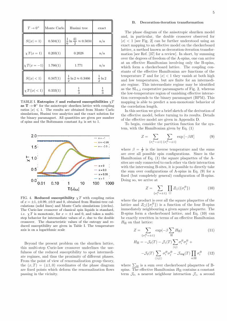
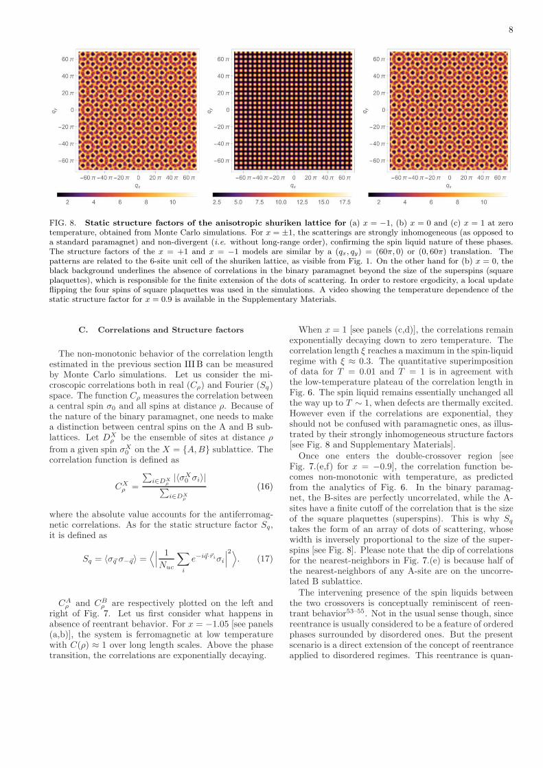
FIG. 8. Static structure factors of the anisotropic shuriken lattice for (a) x = −1, (b) x = 0 and (c) x = 1 at zerotemperature, obtained from Monte Carlo simulations. For x = ±1, the scatterings are strongly inhomogeneous (as opposed toa standard paramagnet) and non-divergent (i.e. without long-range order), confirming the spin liquid nature of these phases.The structure factors of the x = +1 and x = −1 models are similar by a (qx, qy) = (60π, 0) or (0, 60π) translation. Thepatterns are related to the 6-site unit cell of the shuriken lattice, as visible from Fig. 1. On the other hand for (b) x = 0, theblack background underlines the absence of correlations in the binary paramagnet beyond the size of the superspins (squareplaquettes), which is responsible for the finite extension of the dots of scattering. In order to restore ergodicity, a local updateflipping the four spins of square plaquettes was used in the simulations. A video showing the temperature dependence of thestatic structure factor for x = 0.9 is available in the Supplementary Materials.

C. Correlations and Structure factors

The non-monotonic behavior of the correlation lengthestimated in the previous section III B can be measuredby Monte Carlo simulations. Let us consider the mi-croscopic correlations both in real (Cρ) and Fourier (Sq)space. The function Cρ measures the correlation betweena central spin σ0 and all spins at distance ρ. Because ofthe nature of the binary paramagnet, one needs to makea distinction between central spins on the A and B sub-lattices. Let DX

ρ be the ensemble of sites at distance ρ

from a given spin σX0 on the X = A,B sublattice. The

correlation function is defined as

CXρ =

∑

i∈DXρ|〈σX

0 σi〉|∑

i∈DXρ

(16)

where the absolute value accounts for the antiferromag-netic correlations. As for the static structure factor Sq,it is defined as

Sq = 〈σ~q σ−~q〉 =⟨∣

∣

∣

1

Nuc

∑

i

e−i~q·~riσi

∣

∣

∣

2⟩

. (17)

CAρ and CB

ρ are respectively plotted on the left andright of Fig. 7. Let us first consider what happens inabsence of reentrant behavior. For x = −1.05 [see panels(a,b)], the system is ferromagnetic at low temperaturewith C(ρ) ≈ 1 over long length scales. Above the phasetransition, the correlations are exponentially decaying.

When x = 1 [see panels (c,d)], the correlations remainexponentially decaying down to zero temperature. Thecorrelation length ξ reaches a maximum in the spin-liquidregime with ξ ≈ 0.3. The quantitative superimpositionof data for T = 0.01 and T = 1 is in agreement withthe low-temperature plateau of the correlation length inFig. 6. The spin liquid remains essentially unchanged allthe way up to T ∼ 1, when defects are thermally excited.However even if the correlations are exponential, theyshould not be confused with paramagnetic ones, as illus-trated by their strongly inhomogeneous structure factors[see Fig. 8 and Supplementary Materials].Once one enters the double-crossover region [see

Fig. 7.(e,f) for x = −0.9], the correlation function be-comes non-monotonic with temperature, as predictedfrom the analytics of Fig. 6. In the binary paramag-net, the B-sites are perfectly uncorrelated, while the A-sites have a finite cutoff of the correlation that is the sizeof the square plaquettes (superspins). This is why Sq

takes the form of an array of dots of scattering, whosewidth is inversely proportional to the size of the super-spins [see Fig. 8]. Please note that the dip of correlationsfor the nearest-neighbors in Fig. 7.(e) is because half ofthe nearest-neighbors of any A-site are on the uncorre-lated B sublattice.The intervening presence of the spin liquids between

the two crossovers is conceptually reminiscent of reen-trant behavior53–55. Not in the usual sense though, sincereentrance is usually considered to be a feature of orderedphases surrounded by disordered ones. But the presentscenario is a direct extension of the concept of reentranceapplied to disordered regimes. This reentrance is quan-

9

titatively characterized at the macroscopic level by thedouble-peak in the specific heat, the entropy plateau andthe multi-step Curie-law crossover of Fig. 3.(b), and mi-croscopically by the non-monotonic evolution of the cor-relations [see Figs. 6, 7 and 8]. As such, it provides aninteresting mechanism to stabilize a gas-like phase “be-low” a spin liquid, where (a fraction of) the spins formfully correlated clusters which i) can then fluctuate inde-pendently of the other degrees-of-freedom while ii) low-ering the entropy of the gas-like phase below the one ofthe spin liquids.

IV. THE SHURIKEN LATTICE INEXPERIMENTS ?

Finally, we would like to briefly address the exper-imental situation. Unfortunately we are not aware ofan experimental realization of the present model, butseveral directions are possible, each of them with theiradvantages and drawbacks.

The shuriken topology has been observed, albeit quitehidden, in the dysprosium aluminium garnet (DAG)56,57

[see Ref. [58] for a recent review]. The DAG materialhas attracted its share of attention in the 1970’s, but itsmicroscopic Hamiltonian does not respect the geometryof the shuriken lattice – it is actually not frustrated –and is thus quite different from the model presentedin equation (1). However it shows that the shurikentopology can exist in solid state physics.

Cold atoms might offer an alternative. Indeed, thenecessary experimental setup for an optical shurikenlattice has been proposed in Ref. [32]. The idea wasdeveloped in the context of spin-ice physics, i.e. assum-ing an emergent Coulomb gauge theory whose intrinsicIsing degrees of freedom are somewhat different fromthe present model. Nonetheless, optical lattices arepromising, especially if one considers that the inclusionof “proper” Ising spins might be available thanks toartificial gauge fields59.

But the most promising possibility might be artificialfrustrated lattices, where ferromagnetic nano-islands ef-fectively behave like Ising degrees-of-freedom. Since theearly days of artificial spin ice60, many technological andfundamental advances have been made61. In particular,while the thermalization of the Ising-like nano-islandshad been a long-standing issue, this problem is now onthe way to be solved62–68. Furthermore, since the geome-try of the nano-array can be engineered lithographically,a rich diversity of lattices is available, and the shurikengeometry should not be an issue. Concerning the Isingnature of the degrees-of-freedom, nano-islands have re-cently been grown with a magnetization axis ~z perpen-dicular to the lattice69,70.To compute their interaction69,70, let us define the

Ising magnetic moment of two different nano-islands:~S = σ~z and ~S′ = σ′~z. The interaction between themis dipolar of the form

D

(

~S · ~S′

r3− 3

(~S · ~r)(~S′ · ~r)r5

)

=D

r3σ σ′ (18)

where D is the strength of the dipolar interaction and~r is the vector separating the two moments. The result-ing coupling is thus antiferromagnetic and quickly decayswith distance. Hence, at the nearest-neighbour level, aphysical distortion of the shuriken geometry – by elon-gating or shortening the distance between A and B sites –would precisely reproduce the anisotropy of equation (1)for x > 0. However, the influence of interactions beyondnearest-neighbours has successively been found to be ex-perimentally negligible69 and relevant70 on the kagomegeometry. Thus the phase diagram of Fig. 2.(a) couldpossibly be observed at finite temperature, but wouldlikely be influenced by longer-range interactions at rela-tively low temperature.

V. CONCLUSION

The anisotropic shuriken lattice with classical Isingspins supports a variety of different phases as a func-tion of the anisotropy parameter x = JAB/JAA: twolong-range ordered ones for |x| > 1 (ferromagnet andstaggered ferromagnet) and three disordered ones [seeFig. 2]. Among the latter ones, we make the distinction,at zero temperature, between two cooperative paramag-nets SL1,2 for x = ±1, and a phase that we name a binaryparamagnet (BPM) for |x| < 1. The BPM is composedof locally ordered square plaquettes separated by com-pletely uncorrelated single spins on the B-sublattice [seeFig. 2.(d)].At finite temperature, the classical spin liquids SL1,2

spread beyond the singular points x = ±1, giving rise toa double crossover from paramagnet to spin liquid to bi-nary paramagnet, which can be considered as a reentrantbehavior between disordered regimes. This competitionis quantitatively defined by a double-peak feature in thespecific heat, an entropy plateau, a multi-step Curie-lawcrossover and a non-monotonic evolution of the spin-spincorrelation, illustrated by an inhomogeneous structurefactor [see Figs. 3, 4,6, 7 and 8]. The reentrancecan also be precisely defined by the resurgence of thecouplings in the effective checkerboard model [see Fig. 5].

Beyond the physics of the shuriken lattice, the presentwork, and especially Fig. 3, confirms the Husimi-treeapproach as a versatile analytical method to investigatedisordered phases such as spin liquids. Regarding clas-sical spin liquids, Fig. 4 illustrates the usefulness of thereduced susceptibility χT [46], whose temperature evo-lution quantitatively describes the successive crossoversbetween disordered regimes. Last but not least, we

10

hope to bring to light an interesting facet of distortedfrustrated magnets, where extended regions of magneticdisorders can be stabilized by anisotropy, such as on theCairo71,72, kagome51,73 and pyrochlore74 lattices. Suchconnection is particularly promising since it expands thepossibilities of experimental realizations, for example inVolborthite kagome75 or breathing pyrochlores76,77.

Possible extensions of the present work can take differ-ent directions. Motivated by the counter-intuitive emer-gence of valence-bond-crystals made of resonating loopsof size 6 [30], the combined influence of quantum dynam-ics, lattice anisotropy x30,33 and entropy selection pre-sented here should give rise to a plethora of new phasesand reentrant phenomena. As an intermediary step, clas-sical Heisenberg spins also present an extensive degen-eracy at x = 126,33, where thermal order-by-disorderis expected to play an important role in a similar wayas for the parent kagome lattice, especially when tunedby anisotropy x. The addition of an external magneticfield25,29 would provide a direct tool to break the invari-ance by transformation of equation (3), making the phasediagram of Fig. 2.(a) asymmetric. Furthermore, the di-versity of spin textures presented here offers a promisingframework to be probed by itinerant electrons coupled tolocalized spins via double-exchange.

ACKNOWLEDGMENTS

We are thankful to John Chalker, Arnaud Ralko, NicShannon and Mathieu Taillefumier for fruitful discussionsand suggestions. This work was supported by the The-ory of Quantum Matter Unit of the Okinawa Institute ofScience and Technology Graduate University.

Appendix A: Methods

Classical Monte Carlo simulations have been per-formed based on the single-spin-flip algorithm. Let aMonte Carlo step (MCs) be the standard Monte Carlounit of time made of N attempts to flip a spin chosen atrandom. Typical simulations in this paper consist of

• 107 MCs, including 106 MCs for equilibration;

• 1 measurement every 50 MCs for |x| > 1 (total of180 000 samples);

• 1 measurement every 10 MCs for |x| ≤ 1 (total of900 000 samples);

• system sizes varying from N = 2 400 to 15 000.Fig. 2 has been obtained for N = 2 400 sites.

In order to improve the statistics, a large number oftemperatures were simulated, and data were averagedover 4 neighboring temperatures.

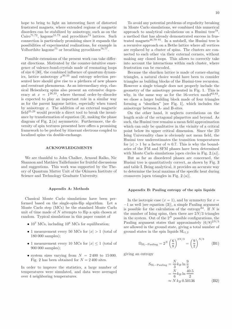
To avoid any potential problems of ergodicity breakingin Monte Carlo simulations, we combined this numericalapproach to analytical calculations on a Husimi tree78,a method that has already demonstrated success in frus-trated magnets46,79–81. In a nutshell, the Husimi tree isa recursive approach on a Bethe lattice where all verticesare replaced by a cluster of spins. The clusters are con-nected to each other via their external corners, withoutmaking any closed loops. This allows to correctly takeinto account the interactions within each cluster, wherefrustration can be encoded.Because the shuriken lattice is made of corner-sharing

triangles, a natural choice would have been to considertriangles as building blocks of the Husimi-tree recursion.However a single triangle does not properly include thegeometry of the anisotropy presented in Fig. 1. This iswhy, in the same way as for the 16-vertex model82,83,we chose a larger building block made of four trianglesforming a “shuriken” [see Fig. 1], which includes theanisotropy between A- and B-sites.On the other hand, it neglects correlations on the

length scale of the octagonal plaquettes and beyond. Assuch, the Husimi tree remains a mean field approximationwhich can only be qualitative in the vicinity of a criticalpoint below its upper critical dimension. Since the 2DIsing Universality class is obviously not mean field, theHusimi tree underestimates the transition temperaturesfor |x| > 1 by a factor of ≈ 0.7. This is why the bound-aries of the FM and SFM phases have been determinedwith Monte Carlo simulations [open circles in Fig. 2.(a)].But as far as disordered phases are concerned, the

Husimi tree is quantitatively correct, as shown by Fig. 3and table I. Being analytical, it provides an accurate wayto determine the local maxima of the specific heat duringcrossovers [open triangles in Fig. 2.(a)].

Appendix B: Pauling entropy of the spin liquids

In the isotropic case (x = 1), and by symmetry for x =−1 as well [see equation (3)], a simple Pauling argumentis possible for the calculation of the entropy84. If N isthe number of Ising spins, then there are 2N/3 trianglesin the system. Out of the 2N possible configurations, thePauling argument states that approximately (6/8)2N/3

are allowed in the ground state, giving a total number ofground states in the spin liquids SL1,2

ΩSL−Pauling = 2N(

6

8

)2N/3

=

(

9

2

)N/3

(B1)

giving an entropy

SSL−Pauling =N

3kB ln

9

2

=N

6kB ln

40.5

2≈ N kB 0.50136 (B2)

11

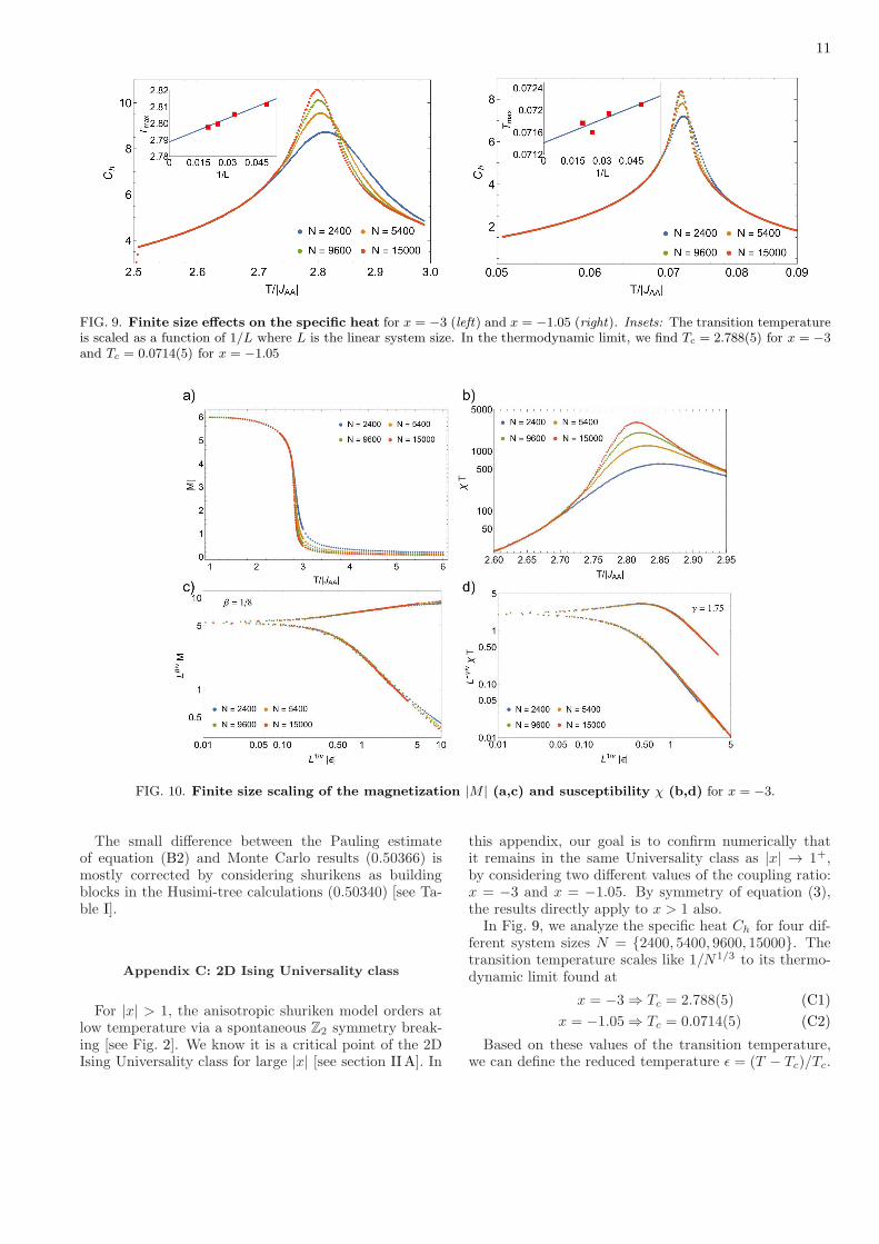
FIG. 9. Finite size effects on the specific heat for x = −3 (left) and x = −1.05 (right). Insets: The transition temperatureis scaled as a function of 1/L where L is the linear system size. In the thermodynamic limit, we find Tc = 2.788(5) for x = −3and Tc = 0.0714(5) for x = −1.05

FIG. 10. Finite size scaling of the magnetization |M | (a,c) and susceptibility χ (b,d) for x = −3.

The small difference between the Pauling estimateof equation (B2) and Monte Carlo results (0.50366) ismostly corrected by considering shurikens as buildingblocks in the Husimi-tree calculations (0.50340) [see Ta-ble I].

Appendix C: 2D Ising Universality class

For |x| > 1, the anisotropic shuriken model orders atlow temperature via a spontaneous Z2 symmetry break-ing [see Fig. 2]. We know it is a critical point of the 2DIsing Universality class for large |x| [see section IIA]. In

this appendix, our goal is to confirm numerically thatit remains in the same Universality class as |x| → 1+,by considering two different values of the coupling ratio:x = −3 and x = −1.05. By symmetry of equation (3),the results directly apply to x > 1 also.In Fig. 9, we analyze the specific heat Ch for four dif-

ferent system sizes N = 2400, 5400, 9600, 15000. Thetransition temperature scales like 1/N1/3 to its thermo-dynamic limit found at

x = −3 ⇒ Tc = 2.788(5) (C1)

x = −1.05 ⇒ Tc = 0.0714(5) (C2)

Based on these values of the transition temperature,we can define the reduced temperature ǫ = (T − Tc)/Tc.

12

FIG. 11. Finite size scaling of the magnetization |M | (a,c) and susceptibility χ (b,d) for x = −1.05.

Following standard finite size scaling85, we confirm inFigs. 10 and 11 that the nature of the phase transitionis consistent with the 2D Ising Universality class withcritical exponents

β = 0.125, γ = 1.75, ν = 1 (C3)

Appendix D: Details of the decoration-iterationtransformation

In this Appendix we give the details of the map tothe effective model on the checkerboard lattice derivedin Section III B. We give the derivation in Section D1and then give details of the calculation of the correlationlength in Section D3.

1. Derivation of the effective model on thecheckerboard lattice

Consider the partition function of the anisotropicshuriken model

Z =∑

σBi =±1

∑

σAi =±1

exp [−β(HAA +HAB)] (D1)

where HAA and HAB are respectively the Hamiltonianof the square plaquettes of A- spins and the Hamiltoniancoupling the intermediate B-spins to the square plaque-

FIG. 12. The checkerboard lattice formed by the set of B-spins on the shuriken lattice.

ttes. Summing over configurations of A- spins, we obtain:

Z =∑

σBi =±1

∏

Z(σBi ) (D2)

where the product is over all the square plaquettes of thelattice and Z(σB

i ) depends on the configuration ofthe four B-spins immediately neighbouring a given squareplaquette.There are sixteen possible arrangements of the four

spins B-spins surrounding a square plaquette of which

13

only four are inequivalent from the point of view of sym- metry. These give rise to four possible values for Z:

Z++++ = 2(2 + 4 cosh(4βJAB) + exp(−4βJAA) + exp(4βJAA) cosh(8βJAB)) (D3)

Z+++− = 2(3 + 3 cosh(4βJAB) + exp(−4βJAA) + exp(4βJAA) cosh(4βJAB)) (D4)

Z++−− = 4(1 + 2 cosh(4βJAB) + cosh(4βJAA)) (D5)

Z+−+− = 4(3 + cosh(4βJAA)) (D6)

From these we can assign “free energies” Fi =−T ln(Zi) to each of the four possible inequivalent con-figurations of B- spins around a square plaquette, i.e.

F++++ = −T ln(Z++++) (D7)

F+++− = −T ln(Z+++−) (D8)

F++−− = −T ln(Z++−−) (D9)

F+−+− = −T ln(Z+−+−) (D10)

The B-spins form a checkerboard lattice as illustratedin Fig. 12. Using Eqs. (D3)-(D10) we can rewriteEq. (D2) in terms of an effective Hamiltonian on thecheckerboard lattice

Z =∑

σBi =±1

exp

[

−β∑

⊠

H⊠

]

(D11)

The sum∑

⊠is a sum over the elementary units of the

checkerboard lattice. The function H⊠ is a function onlyof the four B-spins around a checkerboard unit and re-turns one of the four Fi defined in Eqs. (D7)-(D10) asappropriate to the configuration of those four spins.

We can rewrite H⊠ explicitly in terms of interactionsbetween the spins on the checkerboard lattice. The resul-tant effective Hamiltonian for the spins on the checker-board lattice contains a constant term J0, a nearestneighbour interaction J1, a second nearest neighbour in-teraction J2, and a four-site ring interaction Jring.

H⊠ = −J0(T )− J1(T )∑

〈ij〉

σBi σB

j

−J2(T )∑

〈〈ij〉〉

σBi σB

j − Jring(T )∏

i∈⊠

σBi (D12)

All couplings are functions of temperature Ji = Ji(T ).

The relationship between the temperature dependentcouplings Ji(T ) appearing in Eq. (D12) and the free en-

ergies Fj defined in Eqs. (D7)-(D10) is:

J0 =−1

8(F++++ + F+−+− + 2F++−− + 4F+++−)

(D13)

J1 =−1

8(F++++ − F+−+−) (D14)

J2 =−1

8(F++++ + F+−+− − 2F++−−) (D15)

Jring =−1

8(F++++ + F+−+− + 2F++−− − 4F+++−)

(D16)

We have thus succeeded in mapping the original modelon the shuriken lattice, onto an effective model on thecheckerboard lattice [Eq. (D12)].

2. Transition temperature of the decorated squarelattice

In the limit x → +∞, one obtains the decorated squarelattice. Applying JAA = 0 to Eqs. (D3)-(D10) and theninjecting the results into Eqs. (D14)-(D16), one obtains

J1 =1

2βln(cosh(2βJAB)), (D17)

J2 = Jring = 0. (D18)

The term J0 does not cancel, but it only appears as aprefactor in the partition function of Eq. (D11) and thusdoes not influence the critical point.Our effective model thereby becomes a square lattice

with a temperature dependent nearest-neighbour cou-pling J1(T ). It is exactly soluble and the transition tem-perature Tc = 1/βc is obtained by injecting Eq. (D17)into Onsager’s solution of the Ising square lattice86

βcJ1(Tc) =1

2ln(cosh(2βcJAB))

=1

2ln(

√2 + 1) (Onsager) (D19)

which gives the result of Eq. (4)

Tc =2JAB

ln(√

2 + 1 +√

2 + 2√2)

≈ 1.30841 JAB (D20)

14

3. Correlation length

We observed in Section III B that for x ≤ 1 the cou-plings of the effective model are small compared to thetemperature, for all values of temperature.

An expansion of the partition function of the effectivemodel in powers of βJi is thus justified. Where |x| < 1this expansion is assymptotically exact in both high andlow temperature regimes.

Here we show how to use this expansion to calculatethe correlation function 〈σB

0 σBm〉 for a pair of B-spins.

For simplicity and concreteness we will do the calculationfor a pair separated by a path such as that in Fig. 13,where the shortest route between them traverses only J1

bonds and contains m such bonds. However, there is nodifficulty in making the calculation for other cases.

We have

FIG. 13. A path (in red) between two spins on the checker-board lattice containing only nearest neighbour J1 bonds.The correlation function between two such spins in the disor-dered regime is calculated in section D3.

〈σB0 σB

m〉 =∑

σi±1 σB0 σB

m exp[

β∑

⊠J0(T ) + J1(T )

∑

〈ij〉 σBi σB

j + J2(T )∑

〈〈ij〉〉 σBi σB

j + Jring(T )∏

i∈⊠σBi

]

∑

σi±1 exp[

β∑

⊠J0(T ) + J1(T )

∑

〈ij〉 σBi σB

j + J2(T )∑

〈〈ij〉〉 σBi σB

j + Jring(T )∏

i∈⊠σi

]

=1

Nc

∑

σi±1 σB0 σB

m

∑∞n=0

1n!

[

β∑

⊠J1(T )

∑

〈ij〉 σBi σB

j + J2(T )∑

〈〈ij〉〉 σBi σB

j + Jring(T )∏

i∈⊠σi

]n

1 + 1Nc

∑

σi±1

∑∞n=1

1n!

[

β∑

⊠J1(T )

∑

〈ij〉 σBi σB

j + J2(T )∑

〈〈ij〉〉 σBi σB

j + Jring(T )∏

i∈⊠σBi

]n

(D21)

where Nc is the total number of spin configurations ofthe checkerboard model.The leading non-zero term in Eq. (D21) comes from

the n = m part of the sum in the numerator, and corre-sponds to covering the shortest path between σB

i and σBj

with J1 interactions. There are m! ways of ordering theproduct of terms, which cancels the 1

n! occurring in thedenominator. We thus obtain

〈σBi σB

j 〉 ≈ (βJ1(T ))m

= exp

[

−m ln

(

1

βJ1(T )

)]

(D22)

In our choice of units of length, made such that thelinear size of a unit cell equals 1, the distance betweenthe spins is

r =m√2

(D23)

We therefore have a correlation length

ξBB =1

√2 ln

(

1βJ1(T )

) (D24)

1 L. Savary and L. Balents, Phys. Rev. Lett. 108, 037202(2012).

2 S. B. Lee, S. Onoda, and L. Balents, Phys. Rev. B 86,104412 (2012).

3 Z. Hao, A. G. R. Day, and M. J. P. Gingras, Phys. Rev.B 90, 214430 (2014).

4 A. L. Chernyshev and M. E. Zhitomirsky, Phys. Rev. Lett.113, 237202 (2014).

5 O. Gotze and J. Richter, Phys. Rev. B 91, 104402 (2015).6 J. Oitmaa and R. R. P. Singh,

Phys. Rev. B 93, 014424 (2016).7 K. Essafi, O. Benton, and L. D. C. Jaubert, Nature Com-munications 7, 10297 (2016).

8 L. Messio, B. Bernu, and C. Lhuillier, Phys. Rev. Lett.108, 207204 (2012).

9 Y.-C. He and Y. Chen,Phys. Rev. Lett. 114, 037201 (2015).

10 Y.-C. He, S. Bhattacharjee, F. Pollmann, and R. Moess-ner, Phys. Rev. Lett. 115, 267209 (2015).

11 S. Bieri, L. Messio, B. Bernu, and C. Lhuillier, Phys. Rev.

15

B 92, 060407 (2015).12 Y. Iqbal, H. O. Jeschke, J. Reuther, R. Valentı, I. I. Mazin,

M. Greiter, and R. Thomale, Phys. Rev. B 92, 220404(2015).

13 P. A. McClarty, O. Sikora, R. Moessner, K. Penc, F. Poll-mann, and N. Shannon, Phys. Rev. B 92, 094418 (2015).

14 P. Henelius, T. Lin, M. Enjalran, Z. Hao, J. G. Rau, J. Al-tosaar, F. Flicker, T. Yavors’kii, and M. J. P. Gingras,Phys. Rev. B 93, 024402 (2016).

15 H. D. Zhou, J. G. Cheng, A. M. Hallas, C. R. Wiebe, G. Li,L. Balicas, J. S. Zhou, J. B. Goodenough, J. S. Gardner,and E. S. Choi, Phys. Rev. Lett. 108, 207206 (2012).

16 Z. L. Dun, M. Lee, E. S. Choi, A. M. Hallas, C. R. Wiebe,J. S. Gardner, E. Arrighi, R. S. Freitas, A. M. Arevalo-Lopez, J. P. Attfield, H. D. Zhou, and J. G. Cheng, Phys.Rev. B 89, 064401 (2014).

17 C. R. Wiebe and A. M. Hallas, APL Materials 3, 041519(2015).

18 J. G. Rau and M. J. P. Gingras, Phys. Rev. B 92, 144417(2015).

19 H. Yan, O. Benton, L. D. C. Jaubert, and N. Shannon,arXiv:1311.3501 (2013).

20 L. D. C. Jaubert, O. Benton, J. G. Rau, J. Oitmaa, R. R. P.Singh, N. Shannon, and M. J. P. Gingras, Phys. Rev. Lett.115, 267208 (2015).

21 J. Robert, E. Lhotel, G. Remenyi, S. Sahling,I. Mirebeau, C. Decorse, B. Canals, and S. Petit,Phys. Rev. B 92, 064425 (2015).

22 H. Nakano and T. Sakai, Journal of the Physical Societyof Japan 82, 083709 (2013).

23 R. Siddharthan and A. Georges, Physical Review B 65,014417 (2001).

24 J. Richter, O. Derzhko, and J. Schulenburg, Physical Re-view Letters 93, 107206 (2004).

25 O. Derzhko and J. Richter, The European Physical JournalB 52, 23 (2006).

26 J. Richter, J. Schulenburg, P. Tomczak, and D. Schmal-fuss, Condensed Matter Physics 12, 507 (2009).

27 O. Derzhko, J. Richter, O. Krupnitska, and T. Krokhmal-skii, Phys. Rev. B 88, 094426 (2013).

28 H. Nakano, T. Sakai, and Y. Hasegawa, Journal of thePhysical Society of Japan 83, 084709 (2014).

29 H. Nakano, Y. Hasegawa, and T. Sakai,Journal of the Physical Society of Japan 84, 114703 (2015).

30 A. Ralko and I. Rousochatzakis, Physical Review Letters115, 167202 (2015).

31 P. Tomczak and J. Richter, Journal of Physics A: Mathe-matical and General 36, 5399 (2003).

32 A. W. Glaetzle, M. Dalmonte, R. Nath,I. Rousochatzakis, R. Moessner, and P. Zoller,Phys. Rev. X 4, 041037 (2014).

33 I. Rousochatzakis, R. Moessner, and J. van den Brink,Physical Review B 88, 195109 (2013).

34 O. Derzhko, J. Richter, O. Krupnitska, and T. Krokhmal-skii, Low Temperature Physics 40, 513 (2014), 1312.1111.

35 S. Chun-Feng, K. Xiang-Mu, and Y. Xun-Chang, Com-munications in Theoretical Physics 45, 555 (2006).

36 M. E. Fisher, Phys. Rev. 113, 969 (1959).37 J. Strecka and M. Jascur, Acta Physica Slovaca 65, 235

367 (2015).38 E. H. Lieb, Phys. Rev. Lett. 62, 1201 (1989).39 M. J. Harris, S. T. Bramwell, D. F. McMorrow, T. Zeiske,

and K. W. Godfrey, Phys. Rev. Lett. 79, 2554 (1997).40 J. Villain, Zeitschrift Fur Physik B-Condensed Matter 33,

31 (1979).41 Besides the trivial time-reversal symmetry.42 M. Elhajal, B. Canals, and C. Lacroix,

Phys. Rev. B 66, 014422 (2002).43 B. Canals, M. Elhajal, and C. Lacroix,

Phys. Rev. B 78, 214431 (2008).44 G.-W. Chern, arXiv (2010),

arXiv:1008.3038 [cond-mat.str-el].45 P. A. McClarty, P. Stasiak, and M. J. P. Gingras,

Phys. Rev. B 89, 024425 (2014).46 L. D. C. Jaubert, M. J. Harris, T. Fennell, R. G.

Melko, S. T. Bramwell, and P. C. W. Holdsworth,Phys. Rev. X 3, 011014 (2013).

47 S. V. Isakov, K. S. Raman, R. Moessner, and S. L. Sondhi,Phys. Rev. B 70, 104418 (2004).

48 I. A. Ryzhkin, Journal of Experimental and TheoreticalPhysics 101, 481 (2005).

49 P. H. Conlon and J. T. Chalker, Phys. Rev. B 81 (2010).50 M. Isoda, Journal of Physics: Condensed Matter 20,

315202 (2008).51 W. Li, S.-S. Gong, Y. Zhao, S.-J. Ran, S. Gao, and G. Su,

Phys. Rev. B 82, 134434 (2010).52 A. J. Macdonald, P. C. W. Holdsworth, and R. G. Melko,

Journal of Physics-Condensed Matter 23, 164208 (2011).53 J. Hablutzel, Helv. Phys. Acta 12, 489 (1939).54 V. Vaks, A. Larkin, and Y. N. Ovchinnikov, Soviet Physics

JETP 22, 820 (1966).55 P. Cladis, Molecular Crystals and Liquid Crystals 165, 85 (1988).56 D. P. Landau, B. E. Keen, B. Schneider, and W. P. Wolf,

Phys. Rev. B 3, 2310 (1971).57 W. P. Wolf, B. Schneider, D. P. Landau, and B. E. Keen,

Phys. Rev. B 5, 4472 (1972).58 W. P. Wolf, Brazilian Journal of Physics 30, 794 (2000).59 J. Struck, M. Weinberg, C. Olschlager, P. Wind-

passinger, J. Simonet, K. Sengstock, R. Hoppner,P. Hauke, A. Eckardt, M. Lewenstein, and L. Mathey,Nature Physics 9, 738 (2013).

60 R. F. Wang, C. Nisoli, R. S. Freitas, J. Li, W. McConville,B. J. Cooley, M. S. Lund, N. Samarth, C. Leighton, V. H.Crespi, and P. Schiffer, Nature 439, 303 (2006).

61 C. Nisoli, R. Moessner, and P. Schiffer,Rev. Mod. Phys. 85, 1473 (2013).

62 V. Kapaklis, U. B. Arnalds, A. Harman-Clarke, E. T.Papaioannou, M. Karimipour, P. Korelis, A. Taroni,P. C. W. Holdsworth, S. T. Bramwell, and B. Hjorvarsson,New Journal of Physics 14 (2012), 10.1088/1367-2630/14/3/035009

63 A. Farhan, P. M. Derlet, A. Kleibert, A. Balan, R. V.Chopdekar, M. Wyss, L. Anghinolfi, F. Nolting, and L. J.Heyderman, Nature Physics 9, 1 (2013).

64 A. Farhan, P. M. Derlet, A. Kleibert, A. Balan, R. V.Chopdekar, M. Wyss, J. Perron, A. Scholl, F. Nolting, andL. J. Heyderman, Phys. Rev. Lett. 111, 057204 (2013).

65 J. P. Morgan, J. Akerman, A. Stein, C. Phatak,R. M. L. Evans, S. Langridge, and C. H. Marrows,Phys. Rev. B 87, 024405 (2013).

66 C. Marrows, Nature Physics 9, 324 (2013).67 L. Anghinolfi, H. Luetkens, J. Perron, M. G.

Flokstra, O. Sendetskyi, A. Suter, T. Prokscha,P. M. Derlet, S. L. Lee, and L. J. Heyderman,Nature Communications 6, 8278 (2015).

68 U. B. Arnalds, J. Chico, H. Stopfel, V. Kapak-lis, O. Brenbold, M. A. Verschuuren, U. Wolff,V. Neu, A. Bergman, and B. Hjrvarsson,

16

New Journal of Physics 18, 023008 (2016).69 S. Zhang, J. Li, I. Gilbert, J. Bartell, M. J. Erickson,

Y. Pan, P. E. Lammert, C. Nisoli, K. K. Kohli, R. Misra,V. H. Crespi, N. Samarth, C. Leighton, and P. Schiffer,Phys. Rev. Lett. 109, 087201 (2012).

70 I. A. Chioar, N. Rougemaille, A. Grimm, O. Fruchart,E. Wagner, M. Hehn, D. Lacour, F. Montaigne, andB. Canals, Phys. Rev. B 90, 064411 (2014).

71 I. Rousochatzakis, A. M. Lauchli, and R. Moessner, Phys.Rev. B 85, 104415 (2012).

72 M. Rojas, O. Rojas, and S. M. de Souza, Phys. Rev. E86, 051116 (2012).

73 W. Apel and H.-U. Everts, Journal of Statistical Mechan-ics: Theory and Experiment 2011, P09002 (2011).

74 O. Benton and N. Shannon,Journal of the Physical Society of Japan 84, 104710 (2015).

75 Z. Hiroi, M. Hanawa, N. Kobayashi, M. No-hara, H. Takagi, Y. Kato, and M. Takigawa,Journal of the Physical Society of Japan 70, 3377 (2001).

76 Y. Okamoto, G. J. Nilsen, J. P. Attfield, and Z. Hiroi,

Phys. Rev. Lett. 110, 097203 (2013).77 K. Kimura, S. Nakatsuji, and T. Kimura,

Phys. Rev. B 90, 060414 (2014).78 K. Husimi, Journal of Chemical Physics 18, 682 (1950).79 P. Chandra and B. Doucot, Journal of Physics A-

Mathematical and General 27, 1541 (1994).80 S. Yoshida, K. Nemoto, and K. Wada, Journal of the

Physical Society of Japan 71, 948 (2002).81 J. Strecka and C. Ekiz, Phys. Rev. E 91, 052143 (2015).82 L. Foini, D. Levis, M. Tarzia, and L. Cugliandolo, Journal

of Statistical Mechanics , P02026 (2013).83 D. Levis, L. Cugliandolo, L. Foini, and M. Tarzia, Phys.

Rev. Lett. 110, 207206 (2013).84 L. Pauling, Journal of the American Chemical Society 57,

2680 (1935).85 D. P. Landau and K. Binder, A guide to Monte Carlo sim-

ulation in statistical physics (Cambridge University Press,Berlin, 2009).

86 L. Onsager, Physical Review 65, 117 (1944).