reference gene validation software for improved normalization · pdf filereference gene...
TRANSCRIPT
1/27
Reference gene validation software for improved normalization
J. Vandesompele, M. Kubista, and M. W. Pfaffl
Abstract
Real-time PCR is the method of choice for expression analysis of a limited number of genes. The
measured gene expression variation between subjects is the sum of the true biological variation and
several confounding factors resulting in non-specific variation. The purpose of normalization is to
remove the non-biological variation as much as possible. Several normalization strategies have
been proposed, but the use of one or more reference genes is currently the preferred way of
normalization. While these reference genes constitute the best possible normalizers, a major
problem is that these genes have no constant expression under all experimental conditions. The
experimenter therefore needs to carefully assess whether a certain reference gene is stably
expressed in the experimental system under study. This is not trivial and represents a circular
problem. Fortunately, several algorithms and freely available software have been developed to
address this problem. This chapter aims to provide an overview of the different concepts.
Running title: Reference gene validation strategies
Corresponding author:
Jo Vandesompele
Center for Medical Genetics Ghent
Ghent University Hospital, Medical Research Building
De Pintelaan 185, B-9000 Ghent, Belgium
+32 9 240 5187 (phone) | +32 9 240 6549 (fax)
2/27
Introduction
Real-time PCR has become the de facto standard for mRNA gene expression analysis of a limited
number of genes. Given its large dynamic range of linear quantification, high speed, sensitivity
(low template input required) and resolution (small differences can be measured), this method is
perfectly suited for validation of microarray expression screening results on an independent and
larger sample panel, and for studies of a selected number of candidate genes or pathway
constituents in an experimental setup (biopsies, treated cell cultures or any other sample
collection). More recently, real-time PCR has also entered the high throughput gene expression
analysis field based on 384-well block thermal cyclers and newer platforms, such as array based
devices from Biotrove (http://www.biotrove.com/applications/transcript.asp) and Fluidigm
(http://www.fluidigm.com/biomark.htm) that allow parallel gene expression analysis of even
higher number of genes and samples (1 to 48 samples for 48 to 3072 different genes depending on
platform and configuration).
It is important to realize that any measured variation in gene expression between subjects is caused
by two sources. On the one hand, there‟s the true biological variation, explaining the phenotype or
underlying the phenomenon under investigation. On the other hand, there are several confounding
factors resulting in non-specific variation, including but not limited to template input quantity and
quality, yields of the extraction process and the enzymatic reactions (reverse transcription and
polymerase chain reaction amplification). One of the major difficulties in obtaining reliable
expression patterns is the removal of this experimentally induced non-biological variation from the
true biological variation. This can be done through normalization by controlling as many of the
confounding variables as possible (next section).
Reference genes as golden standard for normalization
There are several strategies to remove experimentally induced variation, each with their own
advantages and considerations (Huggett et al., 2005). While most of these methods cannot
completely reduce all sources of variation, it has been shown to be very important to try to control
all the sources of variation along the entire workflow of PCR based gene expression analysis. If
one does not meticulously try to standardize each step, variation can and will be introduced in your
results that cannot be eliminated by applying the final normalization (Stahlberg et al., 2004). It is
thus recommended to ensure similar sample size for extraction of RNA and to standardize the
amount of RNA for DNase treatment and reverse transcription into cDNA. Furthermore, artificial
RNA molecules can be spiked into the sample prior to extraction or to the RNA extract prior to
reverse transcription (Gilsbach et al., 2006; Huggett et al., 2005; Smith et al., 2003). This will give
an indication of the efficiency of the reverse transcription and qPCR procedures, and will reveal
any inhibition. The spike however, may not be extracted with the same yield as compartmentalized
natural mRNAs and will not control fully for the final amount of input material in the reaction.
Taking everything into consideration, it has been agreed that the reference gene concept is the
currently preferred way of normalizing real-time PCR data (3rd
London qPCR symposium, April
2005). Several companies have identified the problem and provide validated reference gene panels
for various organisms (Table 1). The reference gene concept is particularly attractive because the
reference genes are internal controls that are affected by all sources of variation during the
experimental workflow in the same way as the genes of interest. The reference genes were
expressed in the cells, and their mRNAs are present during prelevation, nucleic acid extraction,
storage, and any enzymatic processes such as DNase treatment and reverse transcription.
3/27
Furthermore, PCR based quantification results for a gene of interest are best normalized using a
factor that is measured using the same methodology (i.e. a reference gene‟s expression is also
measured by PCR).
While the use of reference genes for normalization of gene expression levels is certainly the gold
standard some new approaches for normalization have recently been developed. Argyropoulos et
al. have developed a generic normalization method for real-time PCR against total mRNA. During
reverse transcription this method incorporates a long tailed sequence to each mRNA. After double
stranded cDNA synthesis the tailed sequence can be quantified and is a measure of the mRNA
fraction (Argyropoulos et al., 2006). It remains to be determined what the fraction of mispriming of
the tailed oligo-dT primer is to e.g. highly abundant RNA molecules such as the ribosomal RNAs.
Talaat et al. (2002) and Kanno et al. (2006) use a gene expression normalization strategy based on
DNA. The former measures the DNA content of a total nucleic acids extract by PCR and uses this
as normalization factor. In the latter approach the DNA content is determined spectroscopically,
and the sample is spiked with a cocktail of artificial RNA molecules that is proportional to the
DNA content. These spikes can be used for normalization and also for estimating the transcript
copy number per cell. A major problem with this DNA normalization strategy is that current RNA
extraction protocols are not designed to co-purify DNA, so the extraction yields may be different
between different samples, with the DNA yields being suboptimal. A third alternative to the use of
stably expressed reference genes is the quantification of a specific internal control or so called in
situ calibration (Stahlberg et al., 2003). In these approaches, the investigator does not look for a
stably expressed reference but, based on knowledge about the biological system, selects a gene
whose expression is correlated or anti-correlated with that of the gene of interest. While this
approach does not really allow the comparison of expression levels of a given gene between
samples, it is a powerful approach when the expression ratio of two marker genes is significant for
disease or reflects a biological phenomenon. A final alternative is currently being successfully used
and further explored by Vandesompele and colleagues (unpublished). In this novel approach,
repeat sequences that are expressed in the transcriptome are quantified and assumed to reflect the
amount of total mRNA. Alu repeats are by far the most abundant repeat sequences in the human
genome, and approximately 1,500 human genes contain at least one Alu in their 5‟ or 3‟
untranslated region. The rationale is that differential expression of some genes will not alter the
total expressed Alu repeat content. The current downside is that the Alu repeats are primate
specific, and hence can only be used to normalize primate samples. It is currently under
investigation whether other repeats can be used as references in other organisms.
Software and algorithms for reference gene evaluation and selection
While reference genes have the intrinsic capacity to capture all non-biological variation and as
such constitute the best normalizers, a major problem is that there is substantial evidence in the
literature that most of the commonly used reference genes are regulated under some circumstances.
It is thus of utmost importance to validate in your own experimental situation whether a candidate
reference gene is suitable for normalization. The implications of using an inappropriate reference
gene for real-time reverse transcription PCR data normalization is recently demonstrated by Dheda
et al. (2005). If unrecognized, unexpected changes in reference gene expression can result in
erroneous conclusions about real biological effects. In addition, this type of change often remains
unnoticed because most experiments only include a single reference gene.
Reporting that reference genes might show variable expression under certain conditions is not
really helpful. We therefore need strategies to find proper reference genes, and to implement them
in a sensible normalization procedure. However, it is important to realize that the evaluation of
4/27
expression stability represents a circular problem: How can the expression stability of a candidate
be evaluated if no reliable measure is available to normalize the candidate? This circular problem is
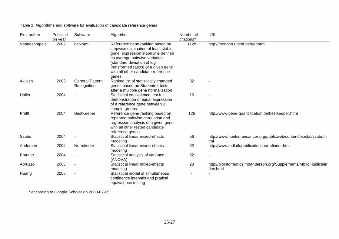
addressed in the following algorithms and Table 2.
geNorm
Vandesompele et al. (2002) were the first to quantify the errors associated with the use of a single
(non-validated) reference gene, to develop a method to select the most stably expressed reference
genes, and to propose the use of multiple reference genes for calculation of a reliable normalization
factor.
As indicated above many studies have reported that reference gene expression can vary
considerably, but Vandesompele et al. (2002) systematically addressed the critical issues of using
reference genes, and proposed an adequate workaround for their variable expression. To this
purpose, they rigorously measured the expression level of 10 common reference genes in 85
samples from 13 different human tissues. Special attention was paid to select genes that belong to
different functional and abundance classes, which significantly reduced the risk that genes are co-
regulated.To determine the errors related to the common practice of using only one reference gene
for normalization, they defined and calculated the single reference gene normalization error as the
ratio of the ratios of two reference genes in two different samples. These analyses clearly
demonstrated that a normalization strategy based on a single (non-validated) reference gene leads
to erroneous expression differences of more than 3- and 6-fold in 25 % and 10 % of the cases,
respectively (with sporadic cases showing errors greater than 20-fold). This clearly warrants the
search for stably expressed genes and an accurate normalization method.
To evaluate the presumed constant expression level of the tested candidate reference genes, a
robust and assumption-free quality parameter was developed based on raw non-normalized
expression levels. The underlying principle is that the expression ratio of two proper reference
genes should be constant across samples. For each reference gene, the pairwise variation with all
other reference genes is calculated as the standard deviation of the logarithmic transformed
expression ratios, followed by the calculation of a reference gene stability value (M value) as the
average pairwise variation of a particular reference gene with all other tested candidate reference
genes.
To manage the large number of calculations, the authors have written a freely available Visual
Basic Application for Microsoft Excel (termed geNorm) that automatically calculates the
expression stability values for any number of candidate reference genes in a set of samples (Table
2). The software employs an algorithm to rank the candidate reference genes according to their
expression stability by a repeated process of stepwise exclusion of the worst scoring reference
gene. Clear expression stability differences were apparent upon comparison of the candidate
reference genes within and between the different tissue panels, which demonstrates that the choice
of a proper reference gene is highly dependent on the tissues or cells under investigation. Because
of the rather large single reference gene normalization errors, and the tissue and gene dependent
expression stability differences, the authors suggest that the geometric mean of multiple reference
genes be calculated as a normalization factor for real-time RT-PCR data. This factor controls for
possible outlying values and abundance differences between the different genes
Finally, the authors outlined a strategy to determine the minimal number of reference genes for
accurate normalization, by variation analysis of normalization factors calculated for an increasing

5/27
number of reference genes. It turned out that three stable genes sufficed for samples with relatively
low expression variation (homogeneous samples), but that other tissues or cell types required a
fourth or fifth reference gene to deal with the observed expression variation. Of course, if one is
only interested in “on versus off” expression, or huge expression differences, there is no need for
normalization using three or more stably expressed reference genes. In contrast, to reliably measure
small expression differences (e.g. 2- to 3-fold) more accurate normalization based on multiple
reference genes is needed.
To validate the accuracy of the proposed RT-PCR normalization method, the authors analyzed
publicly available microarray data and showed that geometric averaging of carefully selected
control genes is equivalent to frequently applied array normalization strategies such as median
ratio normalization and sum of intensity normalization. In a second validation experiment, it is
shown that normalization using the geNorm selected best reference genes result in better removal
of non-biological variation compared to geNorm identified „unstable‟ reference genes.
To evaluate the geNorm ranking Gabrielsson et al. (2005) incorporated a bootstrap step. The
ranking method was bootstrapped by resampling with replacement from the original set of samples.
The resampling procedure was repeated 10,000 times. To check the robustness of the ranking
procedure with respect to outliers, they also repeated the ranking with trimmed standard deviations,
excluding the most outlying 10%, 20%, and 40% of log ratios in the computation of the standard
deviation of the pairwise log ratios. The results obtained by the bootstrap procedure were in
agreement with the original (one pass) geNorm ranking. Furthermore, the ranking was also robust
in that it was essentially unaffected by trimming away 10%, 20%, or 40% of the most outlying log
ratios. This again demonstrates that geNorm allows robust selection of stable reference genes.
In summary, the common practice of non-validated single reference gene normalization results in
relatively large errors. This is a compelling argument for the use of multiple reference genes.
Depending on the observed inherent expression variation of candidate reference genes and the
tissue heterogeneity of the samples under investigation, the geometric mean of the three to five
most stable reference genes allows reliable normalization. The normalization strategy presented is
a prerequisite for accurate RT-PCR expression profiling and provides a first step in determination
of the biological significance of subtle expression differences.
BestKeeper
This Microsoft Excel based program was developed by Pfaffl et al. (2004) and has many feature
similarities with the previously discussed geNorm program (Table 2). The main differences are that
BestKeeper uses Ct values (instead of relative quantities) as input and employs a different measure
of expression stability. The founding principle for identification of stably expressed reference
genes is that proper reference genes should display a similar expression pattern. Hence, their
expression levels should be highly correlated. As such, BestKeeper calculates a Pearson correlation
coefficient for each candidate reference gene pair, along with the probability that the correlation is
significant. All highly correlated (and putatively stably expressed) reference genes are then
combined into an index value (i.e. normalization factor), by calculating the geometric mean. Then,
correlation between each candidate reference gene and the index is calculated, describing the
relation between the index and the contributing reference genes by the correlation coefficient,
coefficient of determination (r2) and the p-value.
6/27
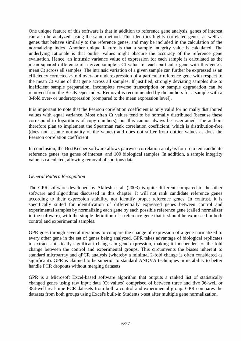
One unique feature of this software is that in addition to reference gene analysis, genes of interest
can also be analyzed, using the same method. This identifies highly correlated genes, as well as
genes that behave similarly to the reference genes, and may be included in the calculation of the
normalizing index. Another unique feature is that a sample integrity value is calculated. The
underlying rationale is that outlier values might obscure the accuracy of the reference gene
evaluation. Hence, an intrinsic variance value of expression for each sample is calculated as the
mean squared difference of a given sample‟s Ct value for each particular gene with this gene‟s
mean Ct across all samples. The intrinsic variation of a given sample can further be expressed as an
efficiency corrected n-fold over- or underexpression of a particular reference gene with respect to
the mean Ct value of that gene across all samples. If justified, strongly deviating samples due to
inefficient sample preparation, incomplete reverse transcription or sample degradation can be
removed from the BestKeeper index. Removal is recommended by the authors for a sample with a
3-fold over- or underexpression (compared to the mean expression level).
It is important to note that the Pearson correlation coefficient is only valid for normally distributed
values with equal variance. Most often Ct values tend to be normally distributed (because these
correspond to logarithms of copy numbers), but this cannot always be ascertained. The authors
therefore plan to implement the Spearman rank correlation coefficient, which is distribution-free
(does not assume normality of the values) and does not suffer from outlier values as does the
Pearson correlation coefficient.
In conclusion, the BestKeeper software allows pairwise correlation analysis for up to ten candidate
reference genes, ten genes of interest, and 100 biological samples. In addition, a sample integrity
value is calculated, allowing removal of spurious data.
General Pattern Recognition
The GPR software developed by Akilesh et al. (2003) is quite different compared to the other
software and algorithms discussed in this chapter. It will not rank candidate reference genes
according to their expression stability, nor identify proper reference genes. In contrast, it is
specifically suited for identification of differentially expressed genes between control and
experimental samples by normalizing each gene by each possible reference gene (called normalizer
in the software), with the simple definition of a reference gene that it should be expressed in both
control and experimental samples.
GPR goes through several iterations to compare the change of expression of a gene normalized to
every other gene in the set of genes being analyzed. GPR takes advantage of biological replicates
to extract statistically significant changes in gene expression, making it independent of the fold
change between the control and experimental groups. This circumvents the biases inherent to
standard microarray and qPCR analysis (whereby a minimal 2-fold change is often considered as
significant). GPR is claimed to be superior to standard ANOVA techniques in its ability to better
handle PCR dropouts without merging datasets.
GPR is a Microsoft Excel-based software algorithm that outputs a ranked list of statistically
changed genes using raw input data (Ct values) comprised of between three and five 96-well or
384-well real-time PCR datasets from both a control and experimental group. GPR compares the
datasets from both groups using Excel's built-in Students t-test after multiple gene normalization.
7/27
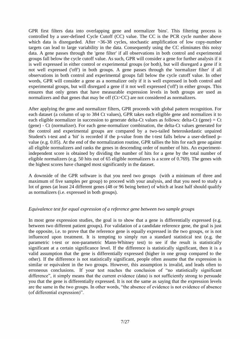
GPR first filters data into overlapping gene and normalizer 'bins'. This filtering process is
controlled by a user-defined Cycle Cutoff (CC) value. The CC is the PCR cycle number above
which data is disregarded. After ~36-38 cycles, stochastic amplification of low copy-number
targets can lead to large variability in the data. Consequently using the CC eliminates this noisy
data. A gene passes through the 'gene filter' if all observations in both control and experimental
groups fall below the cycle cutoff value. As such, GPR will consider a gene for further analysis if it
is well expressed in either control or experimental groups (or both), but will disregard a gene if it
not well expressed ('off') in both groups. A gene passes through the 'normalizer filter' if all
observations in both control and experimental groups fall below the cycle cutoff value. In other
words, GPR will consider a gene as a normalizer only if it is well expressed in both control and
experimental groups, but will disregard a gene if it not well expressed ('off') in either groups. This
ensures that only genes that have measurable expression levels in both groups are used as
normalizers and that genes that may be off (Ct>CC) are not considered as normalizers.
After applying the gene and normalizer filters, GPR proceeds with global pattern recognition. For
each dataset (a column of up to 384 Ct values), GPR takes each eligible gene and normalizes it to
each eligible normalizer in succession to generate delta-Ct values as follows: delta-Ct (gene) = Ct
(gene) - Ct (normalizer). For each gene-normalizer combination, the delta-Ct values generated for
the control and experimental groups are compared by a two-tailed heteroskedastic unpaired
Student's t-test and a 'hit' is recorded if the p-value from the t-test falls below a user-defined p-
value (e.g. 0.05). At the end of the normalization routine, GPR tallies the hits for each gene against
all eligible normalizers and ranks the genes in descending order of number of hits. An experiment-
independent score is obtained by dividing the number of hits for a gene by the total number of
eligible normalizers (e.g. 50 hits out of 65 eligible normalizers is a score of 0.769). The genes with
the highest scores have changed most significantly in the dataset.
A downside of the GPR software is that you need two groups (with a minimum of three and
maximum of five samples per group) to proceed with your analysis, and that you need to study a
lot of genes (at least 24 different genes (48 or 96 being better) of which at least half should qualify
as normalizers (i.e. expressed in both groups).
Equivalence test for equal expression of a reference gene between two sample groups
In most gene expression studies, the goal is to show that a gene is differentially expressed (e.g.
between two different patient groups). For validation of a candidate reference gene, the goal is just
the opposite, i.e. to prove that the reference gene is equally expressed in the two groups, or is not
influenced upon treatment. It is tempting to simply run a standard statistical test (e.g. the
parametric t-test or non-parametric Mann-Whitney test) to see if the result is statistically
significant at a certain significance level. If the difference is statistically significant, then it is a
valid assumption that the gene is differentially expressed (higher in one group compared to the
other). If the difference is not statistically significant, people often assume that the expression is
similar or equivalent in the two groups. However, this assumption is invalid, and leads often to
erroneous conclusions. If your test reaches the conclusion of “no statistically significant
difference”, it simply means that the current evidence (data) is not sufficiently strong to persuade
you that the gene is differentially expressed. It is not the same as saying that the expression levels
are the same in the two groups. In other words, “the absence of evidence is not evidence of absence
(of differential expression)”.
8/27
To address the issue of equivalence testing in real-time PCR based gene expression analysis, Haller
et al. (2004) developed a statistical test for the identification of stably expressed reference genes.
The decision of the test depends on the cutoff used for differential expression. The authors suggest
to use of a 3-fold change as a cutoff. This means that a gene is considered as equivalently
expressed if the expression difference between the two groups is significantly smaller than three.
The authors note that the cutoff should be carefully adjusted to the distribution of each experiment.
In any case, the fold change of a significantly differentially expressed gene of interest after
normalization should be at least the fold change used for the cutoff for evaluation of the reference
genes. The input for the equivalence test (as for any parametric test) should be logarithmized
values (either Ct values or logarithms of quantities derived from a standard curve).
A downside of the current equivalence test is that two sample groups are not always available (e.g.
if one has no prior knowledge of groups, or more than two groups are available). A workaround
could be the development of a one-sample equivalence test (by first rescaling log transformed
expression levels to a mean of 0, and then testing if the expression levels are equivalent or similar
to 0. Another concern is that this test is not entirely assumption-free. The equivalence test assumes
equal amounts of input material in the PCR reaction, which poses a circular problem. As stated in
the introduction of this chapter, the observed reference gene expression variation is not only due to
true biological variation in gene expression, but also to several confounding factors, not taken into
account in the test.
Advanced statistical models
Recently, four papers have been published describing the development and application of advanced
statistical models for describing the expression stability of candidate reference genes. It is beyond
the scope of this chapter to fully explain the underlying mathematics and statistics, but we will
illustrate the different concepts (Table 2).
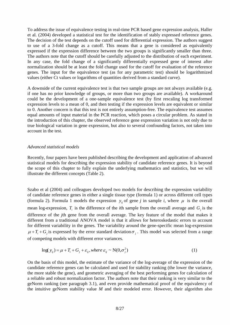
Szabo et al (2004) and colleagues developed two models for describing the expression variability
of candidate reference genes in either a single tissue type (formula 1) or across different cell types
(formula 2). Formula 1 models the expression ijy of gene j in sample i, where is the overall
mean log-expression, iT is the difference of the ith sample from the overall average and jG is the
difference of the jth gene from the overall average. The key feature of the model that makes it
different from a traditional ANOVA model is that it allows for heteroskedastic errors to account
for different variability in the genes. The variability around the gene-specific mean log-expression
ji GT is expressed by the error standard deviation j . This model was selected from a range
of competing models with different error variances.
)N(0,~,)log( 2
jijijjiij whereGTy (1)
On the basis of this model, the estimate of the variance of the log-average of the expression of the
candidate reference genes can be calculated and used for stability ranking (the lower the variance,
the more stable the gene), and geometric averaging of the best performing genes for calculation of
a reliable and robust normalization factor. The authors note that their ranking is very similar to the
geNorm ranking (see paragraph 3.1), and even provide mathematical proof of the equivalency of
the intuitive geNorm stability value M and their modeled error. However, their algorithm also
9/27
ranks the best two reference genes (which geNorm does not do, relying on pairs of genes to
determine stability).
To evaluate the expression stability within and between different tissues, Szabo et al. (2004)
developed formula 2 that models the expression of gene j in the ith sample of tissue-type k, where
denotes the overall mean log-expression, kC is the difference of the kth tissue type from the
overall average, )(kiT is the specific effect of the ith sample from tissue-type k, jG is the difference
of the jth gene from the overall average, and kjCG)( is the tissue-type specific effect of gene j. The
variability comes from two sources: the specific gene ( 2
j ) and the tissue-type ( 2
k ), which are
assumed to be independent and multiplicative.
)N(0,~,)()log( 2
k
2
)()()()( jjkijkikjjkikjki whereCGGTCy (2)
Again, the authors note that their results using model 2 correlate very well with the geNorm
ranking of stability in the different tissues tested in (Vandesompele et al., 2002). A major
advantage of a model based approach however is that the terms are placed within a solid statistical
framework, which allows the algorithm to be generalized to a variety of different experimental
conditions.
For practical performance, both models were fitted using the gls routine of the nlme library for the
freely available statistical language R (http://www.r-project.org/). A step-by-step description of the
procedure as well as the R-script can be found on the authors‟ website (Table 2). Apart from R,
many advanced statistical software programs are able to fit the models (e.g. PROC MIXED from
SAS).
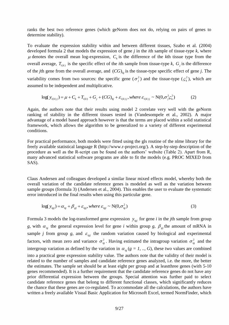
Claus Andersen and colleagues developed a similar linear mixed effects model, whereby both the
overall variation of the candidate reference genes is modeled as well as the variation between
sample groups (formula 3) (Andersen et al., 2004). This enables the user to evaluate the systematic
error introduced in the final results when using this particular gene.
)N(0,~,)log( 2
igigjigjgjigigj wherey (3)
Formula 3 models the log-transformed gene expression igjy for gene i in the jth sample from group
g, with ig the general expression level for gene i within group g, gj the amount of mRNA in
sample j from group g, and igj the random variation caused by biological and experimental
factors, with mean zero and variance 2
ig . Having estimated the intragroup variation 2
ig and the
intergroup variation as defined by the variation in ig (g = 1, .., G), these two values are combined
into a practical gene expression stability value. The authors note that the validity of their model is
related to the number of samples and candidate reference genes analyzed, i.e. the more, the better
the estimates. The sample set should be at least eight per group and at leastthree genes (with 5-10
genes recommended). It is a further requirement that the candidate reference genes do not have any
prior differential expression between the groups. Special attention was further paid to select
candidate reference genes that belong to different functional classes, which significantly reduces
the chance that these genes are co-regulated. To accommodate all the calculations, the authors have
written a freely available Visual Basic Application for Microsoft Excel, termed NormFinder, which
10/27
automatically calculates the stability value for all candidate reference genes (Table 2). In situations
where no single optimal reference gene can be found, the authors suggest to use multiple reference
genes. The rationale is that the variation in the average of multiple genes is smaller than the
variation in individual genes, and that contributions from
reference genes with bias for different groups cancel. A complication is the difficulty of weighting
the relative importance of the intragroup and intergroup variations, and it is possible that the equal
weights used by NormFinder overestimate the cancellation effect. The number of genes to include
in the normalization factor is a trade-off between practical considerations and minimizing the
variation in the normalization factor. The optimal number of genes is reached when addition of a
further gene leads to a negligible reduction in the average of the gene variance estimates.
The above described models use fixed effects for genes and samples and an error model accounting
for gene-specific variability. Abruzzo et al. (2005) and colleagues evaluated several other linear
mixed effects models, including models with random effects to account for sample differences.
The authors conclude that modified versions of the Szabo and Andersen equation that include
either fixed effects (formula 4) or random effects (formula 5) better explain the variability. In
formula 4 a fixed effect ij term is added that represents different expression levels for gene j in
sample i. Formula 5 incorporates a random effect ijC to gene j in sample i. The authors show some
preference for the random effects model (formula 5).
)N(0,~,)log( 2
jijkijkijijijk wherey (4)
)N(0,~ and )N(0,~,)log( 22 ijkjijijkijjijk CwhereCy (5)
The models were fitted using the gls (formula 4) or lme function (formula 5) in S-Plus (Insightful).
Again the authors note that normalization to the geometric mean of the best performing reference
genes result in smaller standard deviations for almost all normalized genes compared to any single
reference gene normalization.
Huang et al. (2006) describe a statistical framework to select a set of reference genes with
approximately constant expression ratios in given tissues or cells. The fundamental difference
between their method and the equivalence test and the linear mixed effects model described earlier
is that their approach identifies genes with relatively constant expressions across tissues while the
other method select genes with absolutely constant expressions. In Huang et al. (2006), the
expression levels of the selected genes may vary across the tissues, but the expression ratios of any
two of the genes should remain relatively constant for every tissue. This is done by testing the (lack
of) parallelism of the lines connecting the mean expressions in the plots where the Y-axis is the log
expression level and the X-axis is the tissue type. Logarithmic gene expression levels are modeled
so that lack of parallelism can be explicitly defined as parameters that can be estimated from
expression data. Furthermore, this method controls the overall error rate by obtaining simultaneous
confidence intervals for these parameters, and a practical equivalence value for gene expression
levels is proposed based on active control genes instead of arbitrarily picking a value as done by
Haller et al., (2004). This active control gene is a differentially expressed gene known to be
involved in the biological phenomenon under investigation.
Formula 6 models the logarithm of expression level ijry for the rth observation on the gene i from
tissue j. ij represents the expected log expressed level of the ith gene in the jth tissue, and ijr the

11/27
experimental error present in the rth observation on the gene i from tissue j (random error with
mean zero).
ijrijijry )log( (6)
Formula 7 measures the lack of parallelism (i.e. absence of interaction of gene i and gene j in tissue
s and k).
ksjiwithjkikjsis
sk
ij ,),()( (7)
The authors try to find those sk
ij values with absolute values small enough to allow the
corresponding reference genes to be used for normalization of gene expression data from the
corresponding tissues. To this purpose, they apply a practical equivalence test. The authors note
that the geNorm stability value is similar to their measure of interaction but without statistical
justification.
Variance of Ct values
A conceptually simple and intuitive way of evaluating reference gene expression stability is the
assessment of the variation of the Ct values for a particular gene across the samples. The higher the
variation, the less stably the gene is expressed in the experimental setup. Dheda et al (2004)
applied this strategy to identify a reference gene with minimal variability under their experimental
conditions. They profiled 13 different candidate reference genes in 28 clinical samples (selected
from a range of different ages, sex and ethnicity to maximize variability). The variation of the
candidate reference genes was visualized using box plots (indicating the median Ct value, the 25
and 75 percentile, and the range), demonstrating clear differences between the genes. The authors
propose a standard deviation of less than 2-fold from the mean expression level of a given gene as
a requirement for suitability as a reference gene (equivalent to a standard deviation of one in Ct
space, assuming 100 % PCR efficiency).
While this method is very simple and will separate the more stable from the less stable genes, it is
not entirely assumption-free, as it assumes equal amounts of input material (something which is
not trivial to guarantee, and what you finally want to correct for using your normalization
procedure, critically touching the circular problem of selecting proper reference genes). In any
case, the variation of the selected (best) reference gene defines the resolution of the final assay
(quantification of the gene of interest). This resolution is dependent on the desired measurement,
e.g. one log variation in reference gene is acceptable to reliably detect a two log difference in target
gene expression.
ANOVA
Brunner et al. (2004) used single-factor ANOVA and linear regression analysis to examine
variation among tissues and RT-PCR experiments. Ct values were analyzed in Microsoft Excel
using single factor ANOVA and regression analysis in the Analysis ToolPak. Assumptions
concerning homogeneity of variance and normality (two requirements to use a parametric ANOVA
procedure) were evaluated from inspection of residuals (the difference between an observed value
and overall mean for all genes) from the ANOVA. The level and significance of the difference

12/27
between gene expression levels in different samples are evaluated by Fisher's F statistic (between-
tissue-sample mean square divided by the error mean square) assuming the three replicate PCR
reactions approximated variance between fully independent observations. The authors further
outline their procedure for data analysis to evaluate candidate reference genes.
In a gene quantification experiment of ten candidate reference genes for different tissues of poplar
trees, examination of the distribution of the residual values from ANOVA indicated that
assumptions concerning homogeneity of variance and normality of data were adequately met. The
ANOVA F-test of differences among tissues indicated that five of the 10 candidate reference genes
showed significant variation in expression among the tissue samples. The mean expression level
for each gene in each tissue sample was regressed against the overall means for the different tissue
samples. This overall mean provides an index of RNA quality and quantity for that tissue sample.
The slope provides an estimate of the degree to which the gene is sensitive to general expression-
promoting conditions, and the residuals (deviation from regression prediction) and mean squared
residuals estimate the degree to which expression of a gene varies unpredictably after linear effects
are removed.
Based on the slope and the coefficient of variation of the regression, the authors define a stability
index as the product of the slope and coefficient of variation. The genes with the lowest stability
index will usually provide the best controls. The authors acknowledge that for some studies, no
single gene may be adequate. In these cases, the geometric mean of two or more of the most stable
reference genes is proposed.
Principal component analysis and autoscaling
Autoscaling is a data pre-treatment process that makes variables of different scales comparable.
Each variable is autoscaled separately by subtracting its mean value and dividing by its standard
deviation (SD). In gene expression analysis we are usually interested in trends of fold changes and
therefore either the logarithm of the expression levels or the Ct values should be autoscaled
(Kubista et al., 2006). This is done by the following formula (with the bar denoting an average):
data raw
gene_A
data raw
gene_A
data raw
gene_Aautoscale
gene_ACtSD
CtCtCt
(8)
The autoscaled expression values for each gene have zero mean and a standard deviation of one.
Hence, in any analysis the genes will be treated as equally important. Whether this is a good
assumption or not is up to the researcher. Essentially, analysis of autoscaled data will classify
samples and genes based on relative changes in expression, while analysis of unscaled (raw) data
also accounts for the magnitudes of the changes in expression. Typically, one does both analyses,
since the two classifications may reveal different relations between samples and/or genes (Leung
and Cavalieri, 2003).
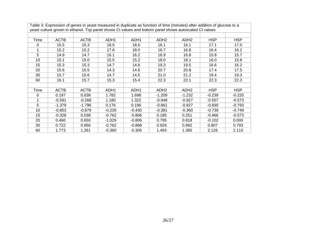
Table 3 shows some data from a study of yeast metabolism (Elbing et al., 2004). Wild-type yeast
was grown with ethanol. As the carbon source, at time zero glucose was added and the expression
of eighteen genes was measured as function of time over 60 minutes. The experiment was repeated
once resulting in duplicate expression profiles. All assays were highly optimized and all genes
were significantly expressed, so there was no need to correct for primer-dimers (Chapter 5).
13/27
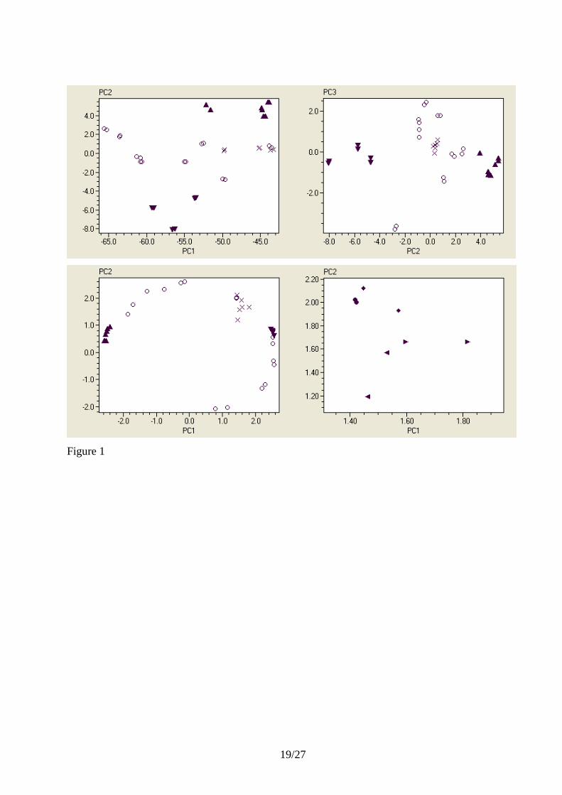
A powerful approach to classify genes and samples based on expression profiles is Principal
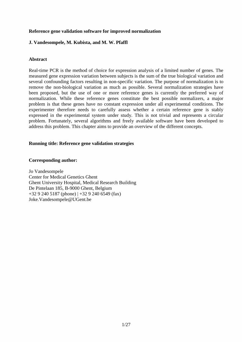
Component Analysis (PCA) (Chapter 5) (Gower, 1971). Figure 1 shows the raw expression
profiles of the yeast genes classified in PC1 vs. PC2 and PC2 vs. PC3 scatter plots. The genes are
represented by different symbols based on their functions. The classification is based on unscaled
Ct values and hence, the overall magnitudes of the changes in the genes‟ expression levels are
important. The mean expression is reflected by PC1, which is the most significant PC, while
variations in expression profiles are contained in the subsequent PC‟s. Inspecting the PC2 vs. PC3
scatter plots we see that the glycolytic and the glucogenetic genes form two clusters that reflect the
common biological functions of its members. Also the candidate reference genes form a cluster.
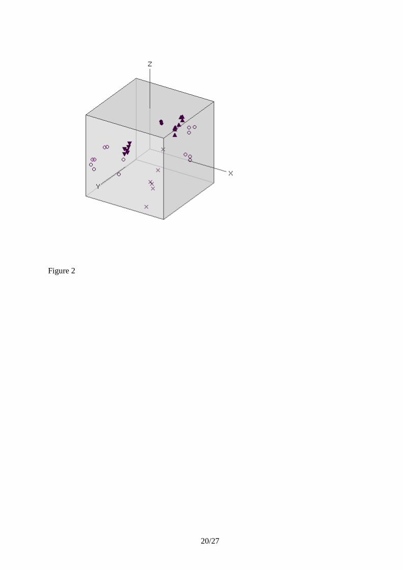
The next step is to autoscale the data. This gives the same weight to all the genes and PCA will
classify them based on their relative changes in expressions. The clusters of the glucogenetic and
glycolytic genes in the PC1 vs. PC2 scatter plot are very tight, and also the candidate reference
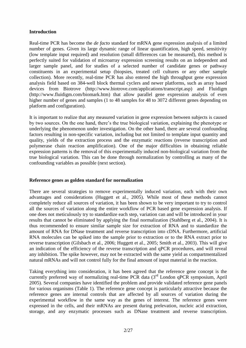
genes form a neat cluster (Figure 2). There is no need to inspect higher order PCs, which are less
informative, when we obtain such nice classification with the two main PCs. In fact, it is quite
common that the PC2 vs. PC3 scatter plot is the most informative for classification of unscaled
data, while the PC1 vs. PC2 scatter plot is the most informative for autoscaled data. The reason is
that autoscaling removes the average response of all genes, which often is not particularly
selective, and is picked up by PC1 of the unscaled data..
So far we have not normalized the expression levels of the genes of interest to any reference genes.
In fact, the candidate reference genes were also classified by the PCA. This is a powerful approach
to test the performance of candidate reference genes before selecting those that will be used for
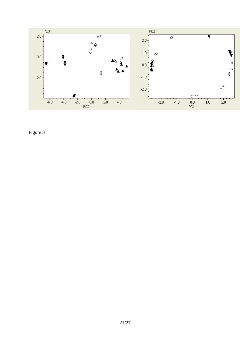
normalization. The right panel in Figure 3 is an enlarged section of the PC1 vs. PC2 scatter plot of
the autoscaled data showing the candidate reference genes. The three candidates show similar
spread of the duplicate samples, indicating they have similar stabilities. Comparing the spread of
replicates in scatter plots is instrumental in assessing the expression stability of genes, but for
stringent comparison the number of biological replicates should be larger. We also see that the
three candidate reference genes cluster around a common center point, with none of them deviating
substantially, suggesting that the responses of the reference genes are not biased. Interestingly, the
heat shock protein (HSP) is located among the candidate reference genes, suggesting that HSP
expression may be invariant in the study. The very tight repeats suggest HSP expression is more
stable than that of the three reference gene candidates, which could make it the preferred choice for
normalization. However, before jumping to that conclusion we must inspect the variation in the
magnitude of HSP expression. In Figure 1 we see that the Ct of HSP varies between 15.7 and 22.3,
which corresponds to 2^(22.3-15.7) = 100-fold variation. This cannot reflect variations in
extraction and reverse transcription yields among the samples. The variation in beta-actin
expression, for example, is only about one Ct, which is 2-fold. Indeed, if we locate HSP in the PC2
vs. PC3 plot of the unscaled data (Figure 1), we see it is very remote from the reference gene
candidates. In fact, it also separates from the reference genes in a PC2 vs. PC3 (not shown) and a
PC1 vs. PC2 vs. PC3 (Figure 2) scatter plot of the autoscaled data. The reason HSP is not
distinguished from the reference gene candidates in lower PC dimensions is that its expression
profile is different from both the glycolytic and glucogenetic genes as well as of the other regulated
genes, and the variation accounted for by the first two PC‟s (90 % based on the eigenvalues) is not
sufficient to explain its deviant behavior.
From the above we conclude that the three candidate reference genes are the best normalizers for
this yeast study. We therefore convert all Ct values to relative quantities (copy numbers) and
normalize with the expression of the reference genes. The conversion requires we assume values
for PCR efficiency and assay sensitivity (Chapter 5). PCA is not particularly sensitive to these

14/27
parameters, and we assume 90 % efficiency and Ct(sc) = 1 for all genes. The copy numbers of the
genes of interest are then normalized with the geometric mean of the expression levels of the three
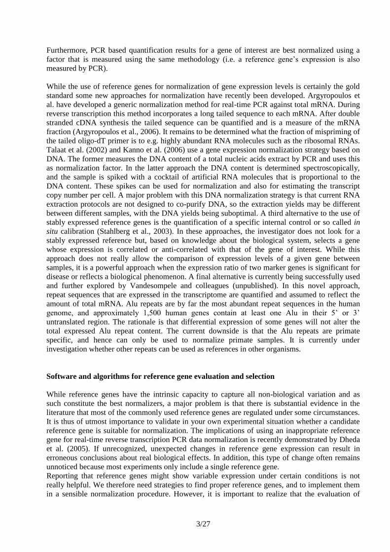
reference genes, and the data are converted back to log2 scale. Finally, the data are analyzed by
PCA (Figure 3). The PC2 vs. PC3 scatter plot of unscaled data clusters the genes based on their
overall changes in expression, while the PC1 vs. PC2 scatter plot of autoscaled data clusters the
genes based on their relative changes in expression. From the scatter plots we identify five groups:
three glucogenetic genes, four glycolytic genes that form a cluster with two of the other genes, a
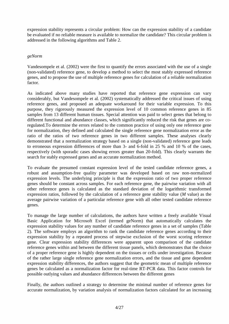
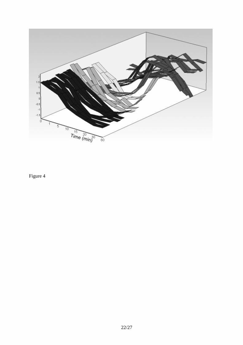
group of other genes, HSP, and one other gene. The autoscaled normalized expression profiles are
also shown in Figure 4.
Clearly, a procedure based on classification of autoscaled and unscaled expression data by PCA to
identify suitable reference genes, followed by normalizing the expression values of the genes of
interest with the expression of the validated reference genes for more detailed classification by
PCA is very powerful. The entire analysis can be performed using dedicated software such as
GenEx from MultiD Analyses (http://www.multid.se). de Kok et al (2005) used PCA in a recent
study to evaluate 13 candidate reference genes.
How important is normalization with reference genes? Comparing the scatter plots of the
normalized data in Figure 3 with the unnormalized data in the top right (unscaled) and bottom left
(autoscaled) panels in Figure 2 we find only minor differences. In fact, autoscaling per se is often
sufficient for classification of expression profiles. In this study, we measured changes in the
expressions of yeast genes as a function of time, and we did not expect important variations in
overall expression levels, extraction and reverse transcription yields. Here, normalization with
reference genes, if poorly chosen, could in fact damage the data by adding noise due to large
random variations in expression levels or due to systematic variation (eg. if HSP had been chosen
as normalizer). For other data, such as clinical samples from different individuals, possibly from
complex tissues and varying disease state the overall expression level and the extraction and
reverse transcription efficiencies may differ substantially among samples making normalization to
reference genes or in situ calibration critical (Stahlberg et al., 2003). Nevertheless, PCA combined
with autoscaling is powerful for selection and validation of candidate reference genes and also for
the classification of the normalized data.
Confirmation of stable expression in qBase
A typical candidate reference gene selection experiment evaluates between five and ten genes, the
more genes studied, the higher the chances for finding stably expressed genes. Once it has been
determined which genes and how many are required for accurate and reliable normalization, this
information can be used for future experiments, as long as no significant changes in the
experimental setup have been introduced. For example, it has been determined that HPRT1,
GAPD and YWHAZ are the most stable control genes for short term cultured human fibroblasts,
these genes can be used for normalization of all future fibroblast samples, as long as culture
conditions, harvesting procedures etc. are kept the same. Nevertheless, it is important to assess the
expression stability of the previously selected reference genes in each new experiment (e.g. when
culturing the cells again, or extract RNA from new (similar) biopsies, or even when synthesizing
new cDNA). This need not be done by re-evaluation all 10 candidate reference genes, but by
assessing the performance of the previously selected and validated reference genes. This is
automatically done in the qBase software (Hellemans et al., unpublished)
(http://medgen.ugent.be/qbase). qBase is a freely available Microsoft Excel based application for
management and analysis of real-time PCR data. The program uses a proven delta-Ct relative

15/27
quantification model with PCR efficiency correction and multiple reference gene normalization.
For each new experiment, qBase aids in the verification of the selected reference genes and
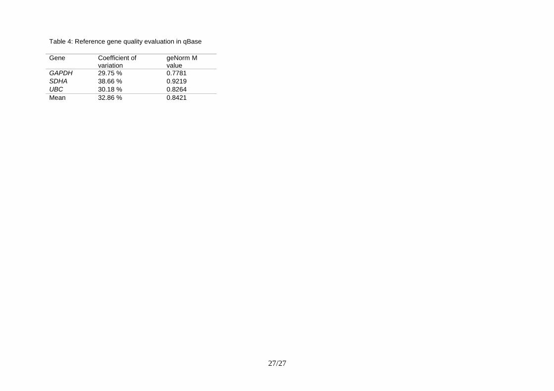
normalization process by means of two reference gene quality evaluation parameters. These can
only be calculated if more than one reference gene is measured. The coefficient of variation
represents the variation of the normalized relative quantities of a reference gene across all samples.
Ideally, the variation after normalization is nil. Hence, lower CV values denote higher stability.
The M value is the gene expression stability parameter as calculated by geNorm. The lower the M
value, the more stably expressed is the reference gene. In table 4 these reference gene quality
parameters are calculated for three stably expressed reference genes in a cancer cell line panel.
As mentioned above the geometric mean of multiple (stably expressed) reference genes is a robust
and accurate normalization factor. Furthermore, inspecting these normalization factors allows you
to inspect possible experimental problems (similar to the integrity index value of the BestKeeper
software). qBase displays the calculated normalization factor (geometric mean of indicated
reference genes) for each sample along with its standard deviation both in tabular form and in a
histogram (Figure 5). Using approximately equal amounts of equal quality input material and
proper reference genes, the normalization factor values should be similar for all samples. High
variability of the normalization factors indicates large differences in starting material quantity or
quality, or a problem with one of the reference gene (either not stably expressed, or not adequately
measured). A variation of 2- to 3-fold is generally seen which is acceptable (this is the non-
biological variation that you want to remove). Any higher variation should be treated with care.
Conclusion
Several strategies have recently been developed to evaluate candidate reference genes for their
suitability as normalizing genes in real-time PCR gene expression quantification experiment. The
methods range from simple and intuitive to advanced and some are available as software programs
or as scripts to facilitate the evaluation or use by any interested readers Scientists often ask what
method they should use to address the issue of reference gene expression stability in their
experimental setup? There is no clear answer.. If there is one lesson to learn from this chapter, it is
that every scientist should at least validate their reference gene(s), the actual method used is less
critical although it should be reported.
In our laboratory, we have analyzed several reference gene data sets over the years (including those
from collaborators or people struggling to interpret their data). We applied several of the above
mentioned algorithms and software programs, and in almost every case, we obtained highly similar
rankings. In a recent study from Willems et al (2006), the authors analyzed their reference gene
expression data using geNorm and NormFinder and came to the same conclusions, namely that no
large differences (except for a few occasional shifts of one or two positions in the obtained
rankings) between geNorm and NormFinder were observed.
16/27
References
Abruzzo, L. V., Lee, K. Y., Fuller, A., Silverman, A., Keating, M. J., Medeiros, L. J., and
Coombes, K. R. (2005). Validation of oligonucleotide microarray data using microfluidic low-
density arrays: a new statistical method to normalize real-time RT-PCR data. Biotechniques 38,
785-792.
Akilesh, S., Shaffer, D. J., and Roopenian, D. (2003). Customized molecular phenotyping by
quantitative gene expression and pattern recognition analysis. Genome Res 13, 1719-1727.
Andersen, C. L., Jensen, J. L., and Orntoft, T. F. (2004). Normalization of real-time quantitative
reverse transcription-PCR data: a model-based variance estimation approach to identify genes
suited for normalization, applied to bladder and colon cancer data sets. Cancer Res 64, 5245-5250.
Argyropoulos, D., Psallida, C., and Spyropoulos, C. G. (2006). Generic normalization method for
real-time PCR. Application for the analysis of the mannanase gene expressed in germinating
tomato seed. FEBS J 273, 770-777.
Brunner, A. M., Yakovlev, I. A., and Strauss, S. H. (2004). Validating internal controls for
quantitative plant gene expression studies. BMC Plant Biol 4, 14.
de Kok, J. B., Roelofs, R. W., Giesendorf, B. A., Pennings, J. L., Waas, E. T., Feuth, T., Swinkels,
D. W., and Span, P. N. (2005). Normalization of gene expression measurements in tumor tissues:
comparison of 13 endogenous control genes. Lab Invest 85, 154-159.
Dheda, K., Huggett, J. F., Bustin, S. A., Johnson, M. A., Rook, G., and Zumla, A. (2004).
Validation of housekeeping genes for normalizing RNA expression in real-time PCR.
Biotechniques 37, 112-114, 116, 118-119.
Dheda, K., Huggett, J. F., Chang, J. S., Kim, L. U., Bustin, S. A., Johnson, M. A., Rook, G. A., and
Zumla, A. (2005). The implications of using an inappropriate reference gene for real-time reverse
transcription PCR data normalization. Anal Biochem 344, 141-143.
Elbing, K., Stahlberg, A., Hohmann, S., and Gustafsson, L. (2004). Transcriptional responses to
glucose at different glycolytic rates in Saccharomyces cerevisiae. Eur J Biochem 271, 4855-4864.
Gabrielsson, B. G., Olofsson, L. E., Sjogren, A., Jernas, M., Elander, A., Lonn, M., Rudemo, M.,
and Carlsson, L. M. (2005). Evaluation of reference genes for studies of gene expression in human
adipose tissue. Obes Res 13, 649-652.
Gilsbach, R., Kouta, M., Bonisch, H., and Bruss, M. (2006). Comparison of in vitro and in vivo
reference genes for internal standardization of real-time PCR data. Biotechniques 40, 173-177.
Gower, J. (1971). Statistical methods of comparing different multivariate analyses of the same
data, In Mathematics in the Archaeological and Historical Sciences, F. Hodson, D. Kendall, and P.
Tautu, eds. (Edinburgh: Edinburgh University Press), pp. 138–149.
Haller, F., Kulle, B., Schwager, S., Gunawan, B., von Heydebreck, A., Sultmann, H., and Fuzesi,
L. (2004). Equivalence test in quantitative reverse transcription polymerase chain reaction:
confirmation of reference genes suitable for normalization. Anal Biochem 335, 1-9.

17/27
Huang, Y., Hsu, J. C., Peruggia, M., and Scott, A. A. (2006). Statistical selection of maintenance
genes for normalization of gene expressions. Stat Appl Genet Mol Biol 5, Article4.
Huggett, J., Dheda, K., Bustin, S., and Zumla, A. (2005). Real-time RT-PCR normalisation;
strategies and considerations. Genes Immun 6, 279-284.
Kanno, J., Aisaki, K., Igarashi, K., Nakatsu, N., Ono, A., Kodama, Y., and Nagao, T. (2006). "Per
cell" normalization method for mRNA measurement by quantitative PCR and microarrays. BMC
Genomics 7, 64.
Kubista, M., Andrade, J. M., Bengtsson, M., Forootan, A., Jonak, J., Lind, K., Sindelka, R.,
Sjoback, R., Sjogreen, B., Strombom, L., et al. (2006). The real-time polymerase chain reaction.
Mol Aspects Med 27, 95-125.
Leung, Y. F., and Cavalieri, D. (2003). Fundamentals of cDNA microarray data analysis. Trends
Genet 19, 649-659.
Pfaffl, M. W., Tichopad, A., Prgomet, C., and Neuvians, T. P. (2004). Determination of stable
housekeeping genes, differentially regulated target genes and sample integrity: BestKeeper--Excel-
based tool using pair-wise correlations. Biotechnol Lett 26, 509-515.
Smith, R. D., Brown, B., Ikonomi, P., and Schechter, A. N. (2003). Exogenous reference RNA for
normalization of real-time quantitative PCR. Biotechniques 34, 88-91.
Stahlberg, A., Aman, P., Ridell, B., Mostad, P., and Kubista, M. (2003). Quantitative real-time
PCR method for detection of B-lymphocyte monoclonality by comparison of kappa and lambda
immunoglobulin light chain expression. Clin Chem 49, 51-59.
Stahlberg, A., Hakansson, J., Xian, X., Semb, H., and Kubista, M. (2004). Properties of the reverse
transcription reaction in mRNA quantification. Clin Chem 50, 509-515.
Szabo, A., Perou, C. M., Karaca, M., Perreard, L., Quackenbush, J. F., and Bernard, P. S. (2004).
Statistical modeling for selecting housekeeper genes. Genome Biol 5, R59.
Talaat, A. M., Howard, S. T., Hale, W. t., Lyons, R., Garner, H., and Johnston, S. A. (2002).
Genomic DNA standards for gene expression profiling in Mycobacterium tuberculosis. Nucleic
Acids Res 30, e104.
Vandesompele, J., De Preter, K., Pattyn, F., Poppe, B., Van Roy, N., De Paepe, A., and Speleman,
F. (2002). Accurate normalization of real-time quantitative RT-PCR data by geometric averaging
of multiple internal control genes. Genome Biol 3, RESEARCH0034.
Willems, E., Mateizel, I., Kemp, C., Cauffman, G., Sermon, K., and Leyns, L. (2006). Selection of
reference genes in mouse embryos and in differentiating human and mouse ES cells. Int J Dev
Biol, 50(7):627-35.
18/27
Tables and Figures
Table 1:Commercial reference gene panels
Table 2:
Algorithms and software for evaluation of candidate reference genes
Table 3:
Expression of genes in yeast measured in duplicate as function of time (minutes) after addition of
glucose to a yeast culture grown in ethanol. Top panel shows Ct values and bottom panel shows
autoscaled Ct values.
Table 4:
Reference gene quality evaluation in qBase
Figure 1
Classification of yeast genes based on PCA presented as scatter plots. Top panels show
classification of unscaled expression profiles (left: PC1 vs. PC2; right: PC2 vs. PC3) and bottom
panels of autoscaled data (left: PC1 vs. PC2; right enlarged section of PC1 vs. PC2). Glucogenetic
(▼), glycolytic (▲), reference candidates (×), HSP (●), and other (○) genes,. In the enlarged
section beta-actin (), PDA (►), IPPI (◄).
Figure 2
PC1 vs. PC2 vs. PC3 scatter plot of autoscaled data. Glucogenetic (▼), glycolytic (▲),reference
candidate (×), HSP (●), and other (○) genes.
Figure 3
Scatter plots of gene expression profiles normalized to the expression of reference genes. PC2 vs.
PC3 unscaled (left) and PC1 vs. PC2 autoscaled (right) data. Glucogenetic (▼), glycolytic (▲),
HSP (●), and other (○) genes.
Figure 4
Autoscaled logarithmic expression profiles of genes of interest normalized to the expression of
reference genes: glycolysis genes (lines 1-8), two other genes with similar profiles (9-12), HSP
(13-14), one other gene (15-16), glycolytic genes (17-22), and one group of other genes (23-30).
Figure 5
qBase normalization factor histogram (geometric mean of three stably expressed reference genes)
for indication of possible experimental problems.
19/27
Figure 1
20/27
Figure 2
21/27
Figure 3
22/27
Figure 4

23/27
Figure 5

24/27
Table 1: Commercial reference gene panels
Company Targeted genera and number of reference genes
URL
Applied Biosystems
Homo (10), Mus (2), Rattus (2), http://www.appliedbiosystems.com
Eurogentec Homo (12), Mus (2), Rattus (1), Oryctolagus (1)
http://www.eurogentec.com
Invitrogen Homo (16), Mus/Rattus (15), Drosophila (2) http://tools.invitrogen.com/content/sfs/brochures/711-022292_LUXhskg_brochure.pdf
PrimerDesign Homo (12), Mus (12), Rattus (12), Caenorhabditis (11), Xenopus (12), Arabidopsis (12), Ovis (12), Danio (12), Bos (7), Sus (10), Nicotiana (6), Cucumis (6), Solenopsis (6)
http://primerdesign.co.uk/genorm_all_species.asp
TATAA Biocenter
Homo (12), Mus (12) http://www.tataa.com/webshop/Endogenous-Control-Panels/View-all-products.html
25/27
Table 2: Algorithms and software for evaluation of candidate reference genes
First author Publication year
Software Algorithm Number of citations*
URL
Vandesompele 2002 geNorm Reference gene ranking based on stepwise elimination of least stable gene; expression stability is defined as average pairwise variation (standard deviation of log transformed ratios) of a given gene with all other candidate reference genes
1128 http://medgen.ugent.be/genorm
Akilesh 2003 General Pattern Recognition
Ranked list of statistically changed genes based on Students t-tests after a multiple gene normalization
32 -
Haller 2004 - Statistical equivalence test for demonstration of equal expression of a reference gene between 2 sample groups
16 -
Pfaffl 2004 BestKeeper Reference gene ranking based on repeated pairwise correlation and regression analysis of a given gene with all other tested candidate reference genes
126 http://www.gene-quantification.de/bestkeeper.html
Szabo 2004 - Statistical linear mixed-effects modeling
56 http://www.huntsmancancer.org/publicweb/content/biostat/szabo.html
Andersen 2004 Normfinder Statistical linear mixed-effects modeling
92 http://www.mdl.dk/publicationsnormfinder.htm
Brunner 2004 - Statistical analysis of variance (ANOVA)
52 -
Abruzzo 2005 - Statistical linear mixed-effects modeling
28 http://bioinformatics.mdanderson.org/Supplements/MicroFluidics/index.html
Huang 2006 - Statistical model of simultaneous confidence intervals and pratical equivalence testing
- -
* according to Google Scholar on 2008-07-05
26/27
Table 3: Expression of genes in yeast measured in duplicate as function of time (minutes) after addition of glucose to a yeast culture grown in ethanol. Top panel shows Ct values and bottom panel shows autoscaled Ct values
Time ACTB ACTB ADH1 ADH1 ADH2 ADH2 HSP HSP
0 15.5 15.3 18.5 18.6 16.1 16.1 17.1 17.0
1 15.2 15.2 17.6 18.0 16.7 16.8 16.4 16.2
5 14.9 14.7 16.1 16.2 16.9 16.8 15.8 15.7
10 15.1 15.0 15.5 15.2 18.0 18.1 16.0 15.8
15 15.3 15.3 14.7 14.6 19.3 19.5 16.6 16.2
20 15.6 15.5 14.3 14.6 20.7 20.8 17.4 17.5
30 15.7 15.6 14.7 14.5 21.0 21.2 19.4 19.3
60 16.1 15.7 15.3 15.4 22.3 22.1 22.3 22.3
Time ACTB ACTB ADH1 ADH1 ADH2 ADH2 HSP HSP
0 0.197 0.038 1.782 1.698 -1.209 -1.232 -0.239 -0.220
1 -0.591 -0.268 1.180 1.322 -0.948 -0.927 -0.557 -0.573
5 -1.379 -1.796 0.176 0.196 -0.861 -0.927 -0.830 -0.793
10 -0.853 -0.879 -0.226 -0.430 -0.381 -0.360 -0.739 -0.749
15 -0.328 0.038 -0.762 -0.806 0.185 0.251 -0.466 -0.573
20 0.460 0.650 -1.029 -0.806 0.795 0.818 -0.102 0.000
30 0.722 0.956 -0.762 -0.868 0.926 0.992 0.807 0.793
60 1.773 1.261 -0.360 -0.305 1.493 1.385 2.126 2.115
27/27
Table 4: Reference gene quality evaluation in qBase
Gene Coefficient of variation
geNorm M value
GAPDH 29.75 % 0.7781
SDHA 38.66 % 0.9219
UBC 30.18 % 0.8264
Mean 32.86 % 0.8421