Brigham Young UniversityDepartment of Electrical and Computer Engineering

459 Clyde BuildingProvo, Utah 84602

Microwave Earth Remote Sensing (MERS) Laboratory

Refinement of SIRF for SASS

Quinn P. Remund

8 June 1998

MERS Technical Report # MERS 98-04ECEN Department Report # TR-L104-98.4

© Copyright 1998, Brigham Young University. All rights reserved.

Re�nement of SIRF for SASS

Quinn P. Remund

Brigham Young University

June 8, 1998

Abstract

The utility of scatterometer data is increased by the scatterometer image re-construction with �lter (SIRF) algorithm. This method uses several passes of thesatellite to e�ectively enhance the spatial resolution of the data. Three parametersof SIRF in uence its ability to converge to the true values and must be tuned whenSIRF is applied to data from di�erent instruments. Initialization values, number ofiterations, and B update weighting all a�ect the performance of SIRF. Originallydeveloped for Seasat-A scatterometer (SASS) data, the algorithm was re�ned forNSCAT and ERS-1/2 AMI scatterometers. With the new knowledge gained fromthese studies, this report addresses the re�nement of SIRF across the three param-eters for SASS data. Synthetic truth images are constructed. SASS measurementdata is simulated using actual SASS data in conjunction with the truth images. Theconvergence properties of SIRF are examined using several statistical measures oferror and correlation. The results indicate that initialization values of Ainit=-8.4dB and Binit=-0.14 dB/deg, 50 iterations, and bacc values of 15 to 20 should beused.

1 Introduction

Remote sensing of the earth's surface from space has proven invaluable in many scienti�cdisciplines. In particular, scatterometers such as the Seasat-A Scatterometer System(SASS) and the NASA Scatterometer (NSCAT) are sensitive to surface parameters.However, the low resolution of these instruments has limited their utility. Recently anew method called the scatterometer image reconstruction with �lter (SIRF) algorithmhas been developed to increase the resolution of the data by using multiple passes of thesatellite over a target region [1]. SIRF is basically a bivariate, nonlinear version of themultiplicative algebraic reconstruction technique. This method produces a maximumentropy solution which is desirable for edge reconstruction in the imagery.

For a limited range of incidence angles, �o is approximately a linear function of �,

10 log10 �o(�) = A+ B(� � 40�) (1)

where A and B are functions of surface characteristics, azimuth angle, and polarization.A is the �o value at 40� incidence and B describes the dependence of �o on �. A and Bprovide valuable information about the surface. SIRF produces images of both A andB.

Several parameters in the SIRF algorithm a�ect its convergence characteristics. Thenumber of iterations, initialization values, and B weighting all in uence the performance

1

of SIRF. The iteration parameter determines how long SIRF iterates to achieve a �nalestimate of the image. Initialization values for both A and B are used to give SIRFa starting estimate of A and B. The SIRF algorithm contains heavy update dampingto avoid noise ampli�cation. This works well in high noise scenarios, but may limitthe ability of the algorithm to converge to the true values in a reasonable number ofiterations when noise levels are lower. For this reason, the B updates are often weightedby a factor (bacc) to accelerate the convergence of SIRF. The original SASS SIRF usesbacc=1.

The algorithm was optimized for NSCAT across all of these parameters by observingthe error and correlation statistics of simulated SIRF images and their ground truthcounterparts [2]. One of the conclusions of this study was to use the global average Aand B values for the initialization. This was chosen to minimize expected convergencetime. Since NSCAT (13.995 GHz) and SASS (14.6 GHz) are both Ku-band instruments,the surface responses should be very similar. For this reason, the same initializationvalues are used for SASS as for NSCAT, namely A=-8.4 dB and B=-0.14 dB/deg.

This report describes a study that re�nes SIRF for SASS data by adjusting theiteration and B weighting parameters. Section 2 discusses the generation of simulatedSASS imagery. Section 3 describes the statistical analysis of these images as comparedwith the truth images. In section 4, the conclusions of the study are given.

2 Generating Simulation Data

To examine the e�ects of the SIRF parameters, synthetic A and B truth images arecreated. The images are created at higher resolution (4.45 km per pixel) than thenominal resolution of the satellite (25 km) with dimensions of approximately 8��8�. Theimages use a rectangular latitude/longitude projection. Two simulations are performedusing the data. The �rst has homogeneous constant truth values A=-10.0 and B=-0.1.The second is a heterogeneous image that illustrates features that are similar to thoseseen in real scatterometer imagery. Figure 1 shows the four truth images used in thisstudy.

SASS L1.5 data records contain geolocation, azimuth angle, incidence angle, and �o

information for each measurement cell. Simulated data is generated using 60 days ofactual SASS data (1978 JD 188-248) taken from the Amazon Basin (latitude range of0.0�S to 8.0�S, longitude range of 55.0�W to 63.0�W) combined with the truth images.The actual data provides geolocation and incidence angle information and the truthimages are used to create synthetic �o values. �o is computed from e�ective A and Bvalues in the measurement footprint (see Figure 2),

Aeff =RkX

c=Lk

TkX

a=Bk

h(x; y; k)Atruth(x; y; k) (2)

Beff =RkX

c=Lk

TkX

a=Bk

h(x; y; k)Btruth(x; y; k) (3)

where Lk, Rk, Tk, and Bk de�ne a bounding rectangle for the kth hexagonal �o mea-surement cell, h(x; y; k) is the weighting function for the (x; y)th resolution element

2

(h(x; y; k)=0 or 1 for NSCAT), Atruth(x; y; k) is the A value for the (x; y)th resolutionelement, and Btruth(x; y; k) is the corresponding B value. The noiseless �o then becomes

�onl = Aeff +Beff (� � 40�): (4)

Realistic noise is added to �onl by using theoretical values of the noise variance. Thesimulated �o is given by

�o = �onl(1 + kp�) (5)

where and � is a zero-mean Gaussian random variable with unity variance. Since noSASS Kp data was available, typical NSCAT Kp values were observed. Figure 3 showshistograms of Kp for several diverse regions throughout the earth. This �gure showsthat Kp rarely exceeds 0.10. Assuming that SASS �o measurements are at most twice asnoisy as NSCAT, four values are used: Kp=0.0 (noiseless),Kp=0.05, Kp=0.10, Kp=0.15,and Kp=0.20. Each of these values is used in simulation for both ground truth scenes.

3 Statistical Analysis of Simulated Images

SIRF was run using the simulated data for all ground truths and all of the selectedKp levels. At each iteration, the resulting reconstructed image was compared with thetruth image. A simple statistical analysis was performed to provide metrics for theperformance of SIRF in all the test scenarios. Several statistical measures were used.In the constant truth simulation, the mean as well as the standard deviation were usedto monitor convergence to the true A and B values. For the heterogeneous case, themean error, error standard deviation, RMS error, and the correlation coe�cient wereused. Each of these provide information about the ability of SIRF to reconstruct thetrue image as a function of iteration number (N) and bacc.

3.1 Constant Truth

For the constant truth simulation, the initialization values used were Ainit=-20.0 andBinit={0.2 to simulate a near worst case situation where the algorithm had a signi�cantdistance to converge. The means and standard deviations were computed after eachiteration for all Kp values. The results are plotted in Figures 4-13.

Figures 4-5 illustrate the noiseless simulation results. The A values converge to thetrue value by the 25th iteration regardless of the bacc value although the bacc=1 plot isbiased a little high. The A standard deviation shows the noise level in the reconstructedimage. This metric converges to a �nal low value. Higher bacc means quicker noise levelreduction. The e�ects of B update weighting are more pronounced in the B error plots.Without B acceleration, SIRF was unable to converge to the true value even after 50iterations. Again, higher bacc means quicker convergence and lower noise level.

As Kp rises, some interesting things begin to happen. First, we observe that regard-less of Kp level, the A mean seems to converge in a very similar manner. The A errornoise level has an increasing noise oor as Kp increases. When Kp=0.05, the standarddeviation appears to converge to this noise oor. However, for higher Kp's the noisein the image is ampli�ed at each iteration diverging from the theoretical oor. For theA statistics, more B weighting yields better results. While B weighting enhances the

3

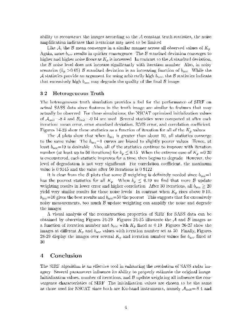
ability to reconstruct the images according to the A constant truth statistics, the noiseampli�cation indicates that iterations may need to be limited.

Like A, the B mean converges in a similar manner across all observed values of Kp.Again, more bacc results in quicker convergence. The B standard deviation converges tohigher and higher noise oors asKp is increased. In contrast to theA standard deviation,the B noise level does not increase signi�cantly with iteration number. Also, in noisyscenarios (kp >0.05) B standard deviation is an increasing function of bacc. While theA statistics provide an argument for using arbitrarily high bacc, the B statistics indicatethat excessively high bacc may degrade the quality of the �nal B image.

3.2 Heterogeneous Truth

The heterogeneous truth simulation provides a feel for the performance of SIRF onactual SASS data since features in the truth image are similar to features that mayactually be observed. For these simulations, the NSCAT optimized initialization valuesof Ainit=-8.4 and Binit=-0.14 are used. Several statistics were computed at after eachiteration: mean error, error standard deviation, RMS error, and correlation coe�cient.Figures 14-23 show these statistics as a function of iteration for all of the Kp values.

The A plots show that when bacc is greater than about 10, all statistics convergeto the same value. The bacc=1 curves are biased to slightly poorer values. Hence, atleast bacc=10 is desirable. Also, all of the statistics continue to improve with iterationnumber (at least up to 50 iterations) for kp � 0:15. When the extreme case of Kp =0.20is encountered, each statistic improves for a time, then begins to degrade. However, thelevel of degradation is not very signi�cant. For correlation coe�cient, the maximumvalue is 0.9145 and the value after 50 iterations is 0.9122.

It is clear from the B plots that some B weighting is de�nitely needed since bacc=1has the poorest statistics for all Kp. When kp � 0:10 we �nd that more B updateweighting results in lower error and higher correlation. After 30 iterations, all bacc � 20yield very similar results for these noise levels. In contrast when Kp rises above 0.10,bacc=10 gives the best results and bacc=50 the poorest. This suggests that for excessivelynoisy measurements, too much B update weighting can amplify the noise and degradethe images.

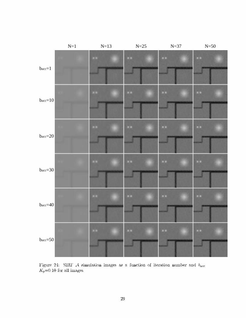
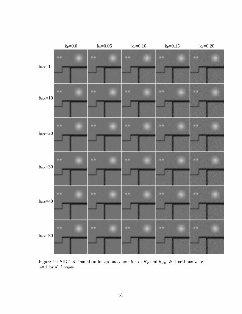
A visual analysis of the reconstruction properties of SIRF for SASS data can beobtained by observing Figures 24-29. Figures 24-25 illustrate the A and B images asa function of iteration number and bacc with Kp �xed at 0.10. Figures 26-27 show theimages at di�erent Kp and bacc values with iteration number set at 50. Finally, Figures28-29 display the images over several Kp and iteration number values for bacc �xed at30.

4 Conclusion

The SIRF algorithm is an e�ective tool in enhancing the resolution of SASS radar im-agery. Several parameters in uence its ability to properly estimate the original image.Initialization values, number of iterations, and B update weighting all in uence the con-vergence characteristics of SIRF. The initialization values are chosen to be the sameas those used for NSCAT since both are Ku-band instruments, namely Ainit=-8.4 and

4

Binit=-0.14. Iteration number is also chosen to be the same as NSCAT since the corre-lation coe�cient and error statistics continue to improve even at the 50th iteration formost cases. The only exception is when Kp=0.20. At this noise level the correlationcoe�cient reaches a maximum then decreases, but only slightly.

The major parameter in need of tuning for SASS is the B update weighting (bacc).It is not clear that the SASS measurement noise is the same as for NSCAT. For thisreason, this study used values that were more than twice as big as typical NSCAT Kp

values. The simulations showed that there is a de�nite need to accelerate the B updatesregardless of noise level since the bacc=1 simulation did not converge to the correct A orB values after 50 iterations. For the A images, increasing bacc only improves the statisticsto a certain point. For example, if bacc� 10 is used, the A error and correlation statisticsare very similar. However, the B statistics tell a di�erent story. WhenKp is low all bacc�20 give similar results. In contrast, when kp � 0.15, more B update weighting meanslower correlation coe�cient. For this reason, it is recommended that an intermediatebacc=15 to 20 be used to balance this trade-o�.

References

[1] D. Long, P. Hardin, and P. Whiting, \Resolution Enhancement of SpaceborneScatterometer Data," IEEE Transactions on Geoscience and Remote Sensing, vol.31, pp. 700{715, 1993.

[2] Q. Remund and D. Long, \Optimization of SIRF for NSCAT," BYU MERS

Technical Report, no. 97-03, July 1997.

5

5 Figures

Figure 1: Truth images used in the SASS SIRF simulations. Top left: constant Aimage (A= -10.0 dB). Top right: constant B image (B= -0.1 dB/deg). Lower left:heterogeneous A image. Lower right: heterogeneous B image.

6

Cross-track

Alo

ng-t

rack

Bounding Rectangle

B

T

L Rkk

k

k

Figure 2: An integrated NSCAT �o cell overlaying the high resolution grid. Only theshaded square grid elements have nonzero h(x;y). The bounding rectangle is also indi-cated.

7

Figure 3: Histograms of Kp for several sample regions over the earth. For each region,both V-pol and H-pol measurements are represented.

8

Figure 4: Simulated SIRF A mean and standard deviations as a function of iterationnumber and bacc for Kp=0.0.

9

Figure 5: Simulated SIRF B mean and standard deviations as a function of iterationnumber and bacc for Kp=0.0.

10

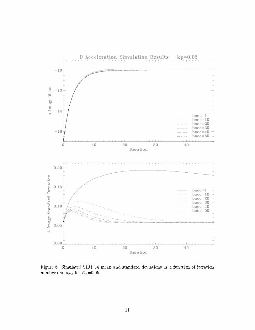
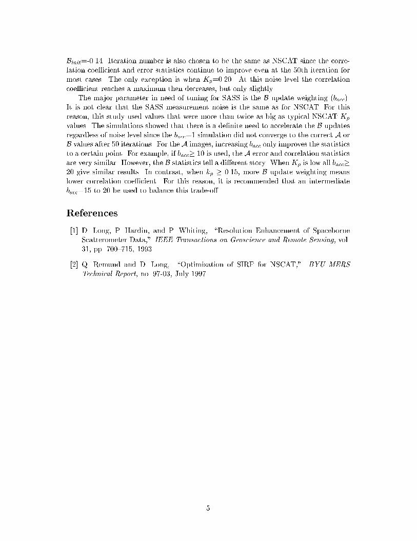
Figure 6: Simulated SIRF A mean and standard deviations as a function of iterationnumber and bacc for Kp=0.05.

11

Figure 7: Simulated SIRF B mean and standard deviations as a function of iterationnumber and bacc for Kp=0.05.

12

Figure 8: Simulated SIRF A mean and standard deviations as a function of iterationnumber and bacc for Kp=0.10.

13

Figure 9: Simulated SIRF B mean and standard deviations as a function of iterationnumber and bacc for Kp=0.10.

14

Figure 10: Simulated SIRF A mean and standard deviations as a function of iterationnumber and bacc for Kp=0.15.

15

Figure 11: Simulated SIRF B mean and standard deviations as a function of iterationnumber and bacc for Kp=0.15.

16

Figure 12: Simulated SIRF A mean and standard deviations as a function of iterationnumber and bacc for Kp=0.20.

17

Figure 13: Simulated SIRF B mean and standard deviations as a function of iterationnumber and bacc for Kp=0.20.

18

Figure 14: Simulated SIRF A error and correlation statistics as a function of iterationnumber and bacc for Kp=0.0.

19

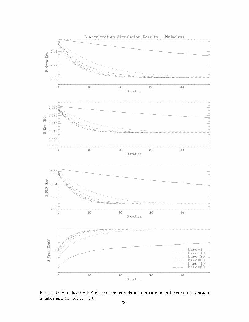
Figure 15: Simulated SIRF B error and correlation statistics as a function of iterationnumber and bacc for Kp=0.0.

20

Figure 16: Simulated SIRF A error and correlation statistics as a function of iterationnumber and bacc for Kp=0.05.

21

Figure 17: Simulated SIRF B error and correlation statistics as a function of iterationnumber and bacc for Kp=0.05.

22

Figure 18: Simulated SIRF A error and correlation statistics as a function of iterationnumber and bacc for Kp=0.10.

23

Figure 19: Simulated SIRF B error and correlation statistics as a function of iterationnumber and bacc for Kp=0.10.

24

Figure 20: Simulated SIRF A error and correlation statistics as a function of iterationnumber and bacc for Kp=0.15.

25

Figure 21: Simulated SIRF B error and correlation statistics as a function of iterationnumber and bacc for Kp=0.15.

26

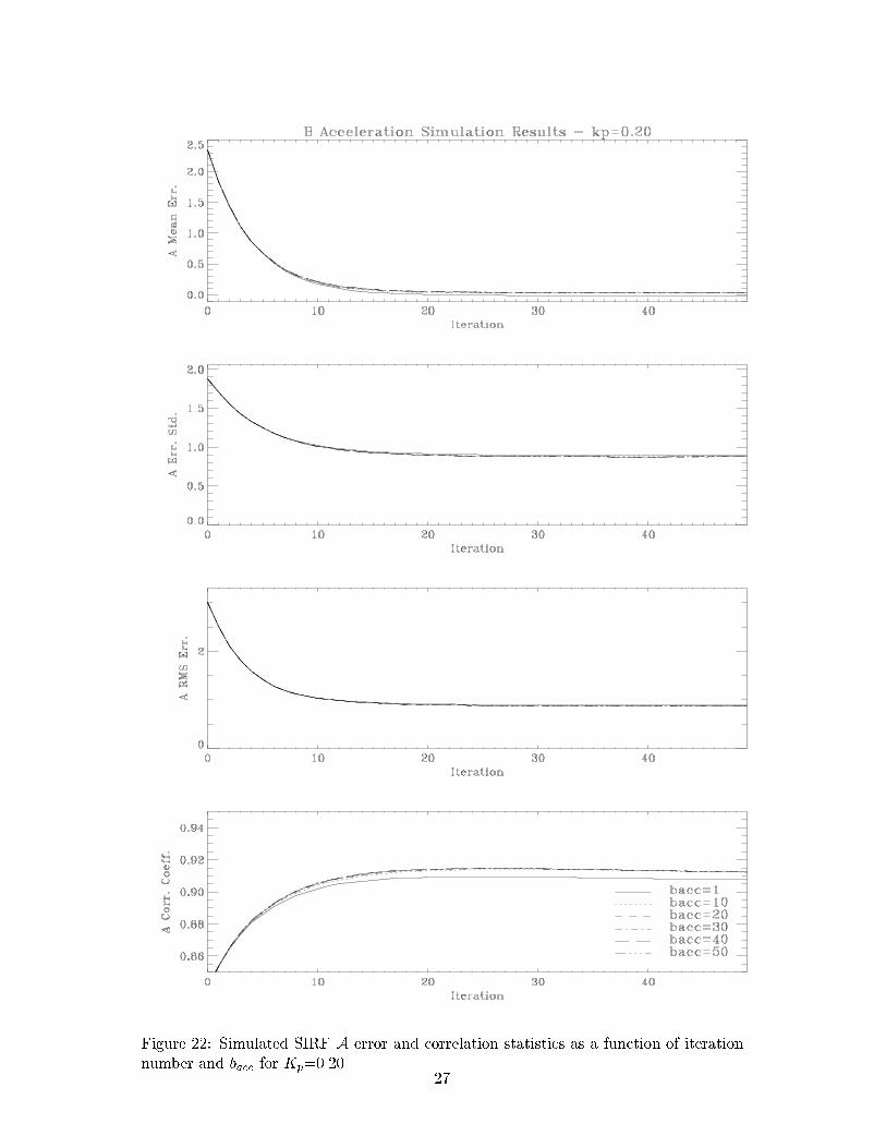
Figure 22: Simulated SIRF A error and correlation statistics as a function of iterationnumber and bacc for Kp=0.20.

27

Figure 23: Simulated SIRF B error and correlation statistics as a function of iterationnumber and bacc for Kp=0.20.

28

N=1 N=13 N=25 N=37 N=50

bacc=1

bacc=10

bacc=20

bacc=30

bacc=40

bacc=50

Figure 24: SIRF A simulation images as a function of iteration number and bacc.Kp=0.10 for all images.

29

N=1 N=13 N=25 N=37 N=50

bacc=1

bacc=10

bacc=20

bacc=30

bacc=40

bacc=50

Figure 25: SIRF B simulation images as a function of iteration number and bacc.Kp=0.10 for all images.

30

kp=0.0 kp=0.05 kp=0.10 kp=0.15 kp=0.20

bacc=1

bacc=10

bacc=20

bacc=30

bacc=40

bacc=50

Figure 26: SIRF A simulation images as a function of Kp and bacc. 50 iterations wereused for all images.

31

kp=0.0 kp=0.05 kp=0.10 kp=0.15 kp=0.20

bacc=1

bacc=10

bacc=20

bacc=30

bacc=40

bacc=50

Figure 27: SIRF B simulation images as a function of Kp and bacc. 50 iterations wereused for all images.

32

kp=0.0 kp=0.05 kp=0.10 kp=0.15 kp=0.20

N=1

N=10

N=20

N=30

N=40

N=50

Figure 28: SIRF A simulation images as a function of Kp and iteration number. bacc=30for all images.

33

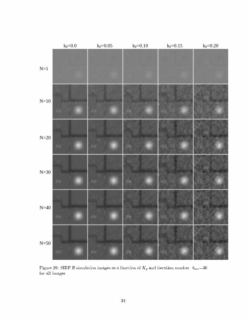
kp=0.0 kp=0.05 kp=0.10 kp=0.15 kp=0.20

N=1

N=10

N=20

N=30

N=40

N=50

Figure 29: SIRF B simulation images as a function of Kp and iteration number. bacc=30for all images.

34