reflection seismic method - university of saskatchewan
TRANSCRIPT

GEOL 335.3
Reflection Seismic Method
Data and Image sort orders;Seismic Impedance;2-D field acquisition geometries;CMP binning and fold;Resolution,Stacking charts;Normal Moveout and correction for it;Stacking;Zero-Offset reflection section;Migration.
Reading:➢ Reynolds, Chapter 6➢ Shearer, 7.1-7.5➢ Telford et al., Sections 4.3, 4.7, 4.8, 4.10

GEOL 335.3
Zero-Offset Section(The goal of reflection imaging)
The ideal of reflection imaging is sources and receivers collocated on a flat horizontal surface (“datum”).
In reality, we have to record at source-receiver offsets, and over complex topography.
Two types of corrections are applied to compensate these factors:
Statics “place” sources and receivers onto the datum; Normal Moveout Corrections “transform” the records into as if they were recorded at collocated sources and receivers.
As a result of these corrections (plus stacking to suppress noise), we obtain a zero-offset section.
Statics compensate
these
NMO correctsfor these

GEOL 335.3
Reflection coefficientQuantity imaged in reflection sections
Z1 = ρ
1VP1
Z2 = ρ
2VP2
At near-normal incidence:P-to-S-wave conversions are negligible;P-wave reflection and transmission amplitudes are determined by the contrast in acoustic impedance Z=ρV (see next page).
P- and S-wave reflection amplitudes usually vary with incidence angles.
Acoustic impedance
RPP=AP reflected
AP incident

GEOL 335.3
Acoustic Impedance
RPP=APreflected
APincident
=Z 2−Z 1
Z 2Z 1
P-wave Reflection Coefficient
P-wave Transmission Coefficient
T PP=1−RPP=2 Z 1
Z 1+Z 2
Reflection-coefficient relations follow from: 1) continuity of displacement, and 2) conservation of energy upon reflection/transmissionAcoustic impedance measures the energy flux within the wave:
Note: if Z2 < Z
1, R<0.
This means polarity reversal upon reflection
E flux=V Edensity=V 2 A2=2
2V A2
Z Kinetic energy
This follows from the continuity of displacement
across the boundary

GEOL 335.3
Acoustic ImpedanceTypical values
From Salisbury, 1996

GEOL 335.3
Spatial resolution
Two points are considered unresolvable when their reflection travel times are separated by less than half the dominant period of the signal: δt < T/2.Therefore,
vertical resolution:
horizontal resolution:
S=R
PP
2P
1
H
z=PP1=4.
x=PP2=H4
2
−H 2≈12
H .
This is calledFresnel Zone radius
Note that horizontal resolution decreases with depth.

GEOL 335.3
Vertical resolution
Faults with different amounts of vertical throws, compared to the dominant wavelength:

GEOL 335.3
Horizontal resolution
Faults with different amounts of vertical throws, compared to the dominant wavelength:

GEOL 335.3
Shot (field) and Common-Midpoint (image) sort orders
Common-Midpoint survey:Helps in reduction of random noise and multiples via redundant coverage of the subsurface;Ground roll is attenuated through the use of geophone arrays.
CMP Fold = 4
CMP spacing = ½ receiver spacing
CMPs
CMP
Geophone arrays:

GEOL 335.3
Field geometry survey and observer's logs,
“chaining notes”
Survey fileProduced by surveyors (usually comes out of GPS unit);
Observer's NotesA record of shooting and recording sequence
➢ Lists shot positions, record (“field file”) numbers (FFIDs), spread positions (“first live station”);
➢ Records weather, interruptions, usual and unusual noise, state of recording system.

GEOL 335.3
Noise (Wave) Test
Conducted prior to the acquisition in order to evaluate the appropriate survey design
Offset range;Noise (ground roll, airwave) characteristics;Offset range for useful reflections.
Ref
lect
ions
Outer traces
Inner traces

GEOL 335.3
Stacking chart
Visualization of source-receiver geometryFixed spread
Split-spread
Marine (off-end)
GEOL 335.3
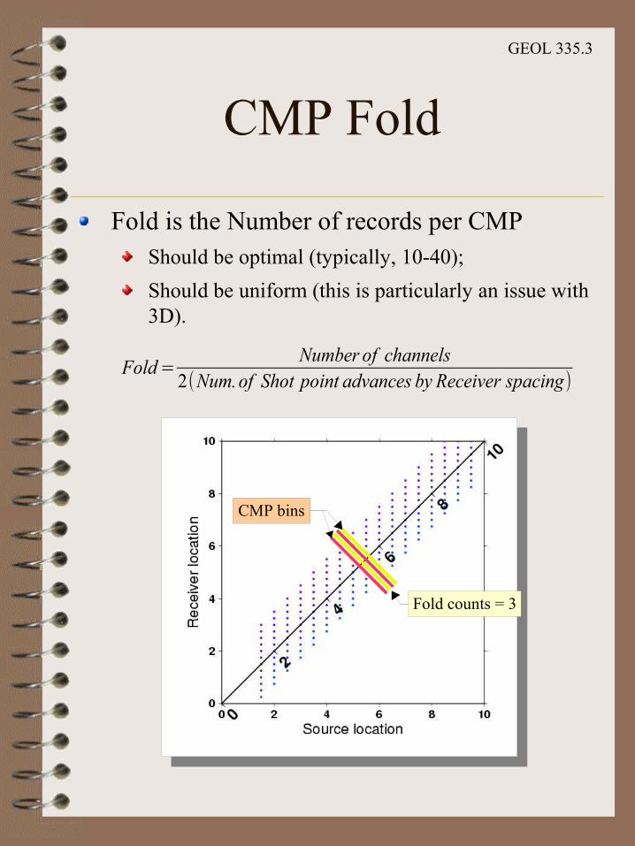
CMP Fold
Fold is the Number of records per CMPShould be optimal (typically, 10-40);Should be uniform (this is particularly an issue with 3D).
Fold counts = 3
Fold =Number of channels
2(Num.of Shot point advances by Receiver spacing)
CMP bins

GEOL 335.3
Crooked-line binningReal seismic lines are often “crooked”CMP bins are then defined for an averaged, smooth line of midpoints

GEOL 335.3
Statics
Statics are time shifts associated with source (∆tS)
and receiver (∆tR) positions
When subtracted ('applied') from the travel-times, place the source and receiver on a common datum.
(Field statics) = (Elevation Correction) + (Weathering Correction);
Elevation correction 'moves' the source and geophone to a common datum surface;Weathering correction removes the effect of slow (~600 m/s) unconsolidated layer.
➢ Obtained from first arrivals, using the plus-minus, GRM, or similar methods.
Where field statics are not accurate enough, residual statics are also applied.
Datumsurface
Weatheredlayer S
GV
W
V>>VW
DS
∆tS
∆tG
t S=ES−DS−Ed
V,
tG= t St uphole
Elevation statics:
Ed
ES

GEOL 335.3
Effects of statics in shot gathers
No statics
Conventionalstatics
GLI(tomography)statics

GEOL 335.3
Effects of statics in stacked image
Conventionalstatics
GLIstatics

GEOL 335.3
Reflection travel-times(Single layer)
t x=4h2 x2
V=
2hV
2
xV
2
=t02
xV
2
t(x) is called (hyperbolic) Normal reflection Moveout (NMO)
Approximation for x << h (parabolic):
t x≈t01
2t0 xV
2
Note that deeper reflections in faster layers
have smaller moveouts
xcritical
S
ic
i V
x
t
Direct
HeadReflected
t0
h
Pre-critical region
Post-critical region

GEOL 335.3
Reflection travel-times(Multiple layers)
where VRMS
is the RMS (root-mean-square) velocity:
h1, V
1, ρ
1
h2, V
2, ρ
2
h3, V
3, ρ
3
h4, V
4, ρ
4
h5, V
5, ρ
5
V6, ρ
6
For multiple layers, t(x) is no longer hyperbolic:
The ray is characterized by ray parameter, p [s/km]
For practical applications (near-vertical incidence, pVi<<1), t(x)
still can be approximated as:
Layer velocities are called
interval velocities
xn p =∑i=1
n hi p V i
1− pV i2≈ p∑
i=1
n
hiV i[112 pV i
2]≈ p∑i=1
n
hiV i ,
t n p =∑i=1
n hi
V i1− pV i2≈∑
i=1
n h i
V i[11
2 pV i
2]=t 012
p2∑i=1
n
h iV i
V RMS=∑i=1
n
hiV i
t0=∑i=1
n
t iV i2
∑i=1
n
ti
.
p=xn p
∑i=1
n
hi V i
,hence:
t nx≈t01
2t0 xV RMS
2

GEOL 335.3
Dipping reflector
For a dipping reflector, the image is smeared up-dip and the stacking velocity is over-estimated.

GEOL 335.3
Measurement of velocities(Velocity analysis)
Reflection (stacking) velocity analysis is usually performed in CMP gathers
because they pertain to specific locations within the subsurface.
Travel-time approach - T2-X2 method: t2(x2) is a linear function. Slope of the graph in t2(x2) diagram is (1/V
Stacking)2.
Waveform approach (velocity spectrum and common velocity stacks (CVS))
stack the records along trial reflection hyperbolas;plot the resulting amplitude in a (time, V
trial)
diagram;pick amplitude peaks - this results in a V(time) profile.

GEOL 335.3
Velocity Spectra
CMP gathers are stacked along trial velocities and presented in time-velocity diagrams.

GEOL 335.3
Common-Velocity Stacks(Velocity analysis)
CMP gathers are NMO-corrected (hyperbolas flattened) using a range of trial velocities and stacked.
Velocities are picked at the amplitude peaks and best resolution in the stacks.

GEOL 335.3
Normal Moveout (NMO) correction
NMO correction transforms a reflection record at offset x into a normal-incidence (x = 0) record:
t x t 0=t x− t NMO
“Stacking velocity”
offset
t
t0
t(x)
0 x1
x2
NMO corrections
Stacking velocity is determined from the data, as a measure of the reflection hyperbola best aligned of with the reflection.
t NMO=t 2− xV
2
−t0≈12t x
V 2

GEOL 335.3
NMO stretch
NMO correction affects the shallower and slower reflections stronger
This is called “NMO stretch”There is a considerable effort in creating “non-stretching” NMO algorithms
Raw NMO corrected
Non-stretchingNMO corrected
Exercise: derive the sensitivities of NMO correction to δt, δV, and δx:
∂ t NMO/∂ t , ∂ t NMO/∂V , ∂ t NMO/∂ x .

GEOL 335.3
Migration
A simplified variant of 'inversion'Transforms the 'time section' into true 'depth image'.
Establishes true positions and dips of reflectors.Collapses diffractions.
Migration collapsesdiffraction curves(surfaces in 3-D)
t rx =t02
xV
2
t d x=t 0
2
t0
22
xV
2

GEOL 335.3ModelingDepth-velocity model
Reflections from the top of salt layer
Reflections from the base of salt layer
Ray tracing to determine stacking velocities
Salt

GEOL 335.3
Synthetic seismogramsAcoustic log
Synthetics(Convolved with
wavelet)Field dataafter NMO
Synthetics with
principalmultiples
Synthetics is spliced into CMP sectionfor comparison
Proceed